1 Introduction
We have recently proposed (de Carvalho Reference de Carvalho2016) that a gas of relativistic electrons, in the long wavelength limit, for weak external fields and neglecting electron–electron (
 $e{-}e$
) interactions, exhibits Drude-like expressions for both electric and magnetic responses. We then argued that the relativistic electron gas represents a natural realization of a material with simultaneously negative electric permittivity
 $\unicode[STIX]{x1D716}$
and magnetic permeability
 $\unicode[STIX]{x1D707}$
(Veselago Reference Veselago1968), (Pendry Reference Pendry2003).
As a test on the accuracy of our approximations (long wavelength, weak external fields, no
 $e{-}e$
interactions), we have compared our predictions with non-relativistic data from metallic systems (Reyes-Gómez & de Carvalho Reference Reyes-Gómez, Oliveira and de Carvalho2016) and found that their quasi-free electrons exhibited responses that agreed well with the theoretical calculations at finite temperature, giving good estimates for physical quantities such as plasma frequencies. Clearly, the relativistic electron gases found in synchrotron beams or in astrophysical scenarios are examples of physical systems required to complete the verification of our theoretical predictions.
Quantum electrodynamics (QED) at finite temperatures and finite particle densities provides a unified treatment that relates electromagnetic responses to the well-known polarization tensor (Akhiezer & Peletminskii Reference Akhiezer and Peletminskii1960) with both vacuum and medium contributions. Thanks to that treatment, it has been established (de Carvalho Reference de Carvalho2016) that (i) all responses depend on three scalar functions (one for the vacuum; two for the medium), (ii) polarizations depend on both the electric and magnetic fields, just as magnetizations depend on both magnetic and electric fields and (iii) many aspects of the analysis of electric responses will carry over to the magnetic ones, due to the analogy between permittivities
 $\unicode[STIX]{x1D716}$
and inverse permeabilities
 $\unicode[STIX]{x1D708}\equiv \unicode[STIX]{x1D707}^{-1}$
, among them the fact that both
 $\unicode[STIX]{x1D716}$
and
 $\unicode[STIX]{x1D708}$
exhibit Drude-like responses at low frequencies in the long wavelength limit.
The present article calculates the real and imaginary parts of the electromagnetic responses of relativistic electrons. At temperatures
 $T\neq 0$
, the problem is reduced to one-dimensional (1-D) integrals which involve the Fermi–Dirac occupation numbers for electrons and positrons. At
 $T=0$
, however, as the occupation numbers become step functions, we obtain analytic expressions for the medium contributions.
Analytic results for the response functions of the relativistic electron gas at
 $T=0$
have already appeared in the literature in the context of plasma physics (Jancovici Reference Jancovici1962; Melrose & Hayes Reference Melrose and Hayes1984; Barton Reference Barton1990; Pulsifer & Kalman Reference Pulsifer and Kalman1992; Barbaro & Quaglia Reference Barbaro, Cenni and Quaglia2005; McOrist & Weise Reference McOrist, Melrose and Weise2007; Eliasson & Shukla Reference Eliasson and Shukla2011). Only expressions for the longitudinal and transverse parts of the electric permittivity,
 $\unicode[STIX]{x1D716}_{L}$
and
 $\unicode[STIX]{x1D716}_{T}$
, were derived.
It is worth noting that, in the non-relativistic case, electromagnetic responses depend on two independent functions, so that magnetic responses may be obtained from
 $\unicode[STIX]{x1D716}_{L}$
and
 $\unicode[STIX]{x1D716}_{T}$
. In the relativistic case, however, responses depend on three independent functions, one of which accounts for the vacuum contribution. It turns out that the vacuum contribution is negligible at low frequencies for typical electron densities, so one can obtain magnetic responses from electric ones.
Nonetheless, one might envisage situations of extremely low densities where the vacuum contributes at low frequencies. Also, at high frequencies, it does play a role. Thus, we present analytic results at
 $T=0$
and numerical ones at
 $T\neq 0$
for electric permittivities and for magnetic permeabilities.
It should also be noted that finite temperature and density QED has been used by several authors to compute electromagnetic responses (Tsai & Erber Reference Tsai and Erber1974; Pérez Rojas & Shabad Reference Pérez Rojas and Shabad1982; Weldon Reference Weldon1982; Donoghue & Robinett Reference Donoghue, Holstein and Robinett1985; Ahmed & Masood Reference Ahmed and Masood1991; Masood & Saleem Reference Masood and Saleem2016). Nevertheless, those articles do not obtain analytic expressions at
 $T=0$
and concentrate on some limiting cases for
 $T\neq 0$
.
Electromagnetic responses may be used to obtain the dispersion relation for plasmon modes that propagate when external electromagnetic fields induce resonant charge density collective oscillations in the electron gas. Such modes are present even when we neglect electron–electron interactions, as is well established in the condensed matter (Abrikosov & Dzyaloshinski Reference Abrikosov, Gorkov and Dzyaloshinski1975; Ashcroft & Mermin Reference Ashcroft and Mermin2005; Fetter & Walecka Reference Fetter and Walecka2012) and finite temperature field theory (Le Bellac Reference Le Bellac2000; Kapusta & Gale Reference Kapusta and Gale2006) literatures.
In the particular case of longitudinal electric plasmon modes, used here as an example, the condition
 $\unicode[STIX]{x1D716}_{L}=0$
leads to the desired dispersion relation, so we obtain the corresponding curve in the frequency–wavenumber plane. Furthermore, when the plasmon dispersion curve reaches the region where
 $\unicode[STIX]{x1D716}_{L}$
acquires an imaginary part, the plasmon decays into an electron–hole pair, with the hole corresponding to the absence of an electron in the Fermi sea (the region between
 $mc^{2}$
and the Fermi energy
 $\unicode[STIX]{x1D700}_{F}$
) (Sturm & Oliveira Reference Sturm and Oliveira1980, Reference Sturm and Oliveira1981; Sturm Reference Sturm1982). The imaginary part of
 $\unicode[STIX]{x1D716}_{L}$
allows for the calculation of decay times.
The article is organized as follows: Section 2 derives electromagnetic responses from the polarization tensor of QED and expresses them in terms of three scalar functions. Section 3 derives the imaginary and real parts of the response functions for
 $T\neq 0$
in terms of 1-D integrals and in terms of analytic expressions for
 $T=0$
. Section 4 connects electromagnetic responses to collective plasmon excitations to obtain their dispersion relations. Finally, Section 5 presents our conclusions. Appendices A–D give details of the calculations in Section 3.
2 Electromagnetic responses from QED
A semiclassical expansion for the partition function
 $Z$
of QED at finite temperature
 $T$
with electron chemical potential
 $\unicode[STIX]{x1D709}$
was derived in de Carvalho (Reference de Carvalho2016). Its starting point was the expression for
 $Z$
in terms of a path integral over the electromagnetic gauge fields and the electron fermionic fields, minimally coupled. The imaginary time formalism was used to implement the finite temperature condition. Throughout the derivation, natural units
 $\hbar =1$
,
 $c=1$
and
 $k_{B}=1$
were used.
The gauge field was then written as the sum of a classical field and a fluctuating quantum field. The quadratic integral over the quantum gauge field was performed giving rise to an effective Lagrangian with an electron–electron interaction term mediated by photons (the Coulomb interaction) and a lowest-order (in the quantum gauge field) term describing the electrons in interaction with the classical field. Integrating over the electron field yielded a fermionic determinant which was expanded in the classical gauge field, assumed to be weak. Only the lowest-order term in the expansion was kept, which is equivalent to the linear response approximation, and the electron–electron interaction was neglected, as it gave rise to higher-order terms in
 $\unicode[STIX]{x1D6FC}\equiv \text{e}^{2}/(4\unicode[STIX]{x03C0})=1/137$
.
We were thus able to write an effective action for the classical gauge field. We extremized it to obtain equations of motion that took into account the presence of the medium. The overall effect was to add an induced current as a source for Maxwell’s equations, which in turn led to the polarization and magnetization of the electron gas through the momentum-space equation
 $$\begin{eqnarray}\text{i}q_{\unicode[STIX]{x1D707}}\tilde{P}_{\unicode[STIX]{x1D707}\unicode[STIX]{x1D708}}(q)=\tilde{\unicode[STIX]{x1D6F1}}_{\unicode[STIX]{x1D708}\unicode[STIX]{x1D70E}}(q)\tilde{A}_{\unicode[STIX]{x1D70E}}(q).\end{eqnarray}$$
The Euclidean space
 $P_{\unicode[STIX]{x1D707}\unicode[STIX]{x1D708}}$
encodes the polarization
 $\boldsymbol{P}$
(
 $P_{4j}=\text{i}P_{j}$
) and magnetization
 $\boldsymbol{M}$
(
 $P_{ij}=-\unicode[STIX]{x1D716}_{ijk}M_{k}$
) vectors.
 $\tilde{\unicode[STIX]{x1D6F1}}_{\unicode[STIX]{x1D708}\unicode[STIX]{x1D70E}}(q)$
is the one-loop polarization tensor of QED (Akhiezer & Peletminskii Reference Akhiezer and Peletminskii1960)
 $$\begin{eqnarray}\tilde{\unicode[STIX]{x1D6F1}}_{\unicode[STIX]{x1D707}\unicode[STIX]{x1D708}}=-\frac{\text{e}^{2}}{\unicode[STIX]{x1D6FD}}\mathop{\sum }_{n=-\infty }^{+\infty }\int \frac{\text{d}^{3}p}{(2\unicode[STIX]{x03C0})^{3}}\text{Sp}[\unicode[STIX]{x1D6FE}_{\unicode[STIX]{x1D707}}G_{0}(p)\unicode[STIX]{x1D6FE}_{\unicode[STIX]{x1D708}}G_{0}(p-q)],\end{eqnarray}$$
where
 $\unicode[STIX]{x1D6FD}=T^{-1}$
, the sum is over Matsubara frequencies
 $p_{4}=(2n+1)\unicode[STIX]{x03C0}T$
,
 $G_{0}$
is the free electron propagator and Sp denotes trace over Dirac matrices. Equation (2.1) implies
 $$\begin{eqnarray}\tilde{P}_{\unicode[STIX]{x1D707}\unicode[STIX]{x1D708}}=\frac{\tilde{\unicode[STIX]{x1D6F1}}_{\unicode[STIX]{x1D707}\unicode[STIX]{x1D70E}}}{q^{2}}\tilde{F}_{\unicode[STIX]{x1D708}\unicode[STIX]{x1D70E}}-\frac{\tilde{\unicode[STIX]{x1D6F1}}_{\unicode[STIX]{x1D708}\unicode[STIX]{x1D70E}}}{q^{2}}\tilde{F}_{\unicode[STIX]{x1D707}\unicode[STIX]{x1D70E}},\end{eqnarray}$$
so that polarization and magnetization are related to the fields
 $\boldsymbol{E}$
(
 $\tilde{F}_{4j}=\text{i}\tilde{E}^{j}$
) and
 $\boldsymbol{B}$
(
 $\tilde{F}_{ij}=\unicode[STIX]{x1D716}_{ijk}\tilde{B}^{k}$
), thus yielding electric and magnetic susceptibilities and, ultimately, electric permittivities and magnetic permeabilities.
One may write
 $\tilde{\unicode[STIX]{x1D6F1}}_{\unicode[STIX]{x1D708}\unicode[STIX]{x1D70E}}=\tilde{\unicode[STIX]{x1D6F1}}_{\unicode[STIX]{x1D708}\unicode[STIX]{x1D70E}}^{(v)}+\tilde{\unicode[STIX]{x1D6F1}}_{\unicode[STIX]{x1D708}\unicode[STIX]{x1D70E}}^{(m)}$
to separate vacuum (
 $T=\unicode[STIX]{x1D709}=0$
) and medium contributions. The vacuum contribution has the structure
 $$\begin{eqnarray}-\frac{\tilde{\unicode[STIX]{x1D6F1}}_{\unicode[STIX]{x1D708}\unicode[STIX]{x1D70E}}^{(v)}}{q^{2}}=\left(\unicode[STIX]{x1D6FF}_{\unicode[STIX]{x1D708}\unicode[STIX]{x1D70E}}-\frac{q_{\unicode[STIX]{x1D708}}q_{\unicode[STIX]{x1D70E}}}{q^{2}}\right){\mathcal{C}}(q^{2}).\end{eqnarray}$$
The medium, however, introduces a preferred reference frame (that of its centre of mass). The symmetry of the problem is then reduced to three-dimensional rotation and gauge invariance, leading to
 $$\begin{eqnarray}-\frac{\tilde{\unicode[STIX]{x1D6F1}}_{ij}^{(m)}}{q^{2}}=\left(\unicode[STIX]{x1D6FF}_{ij}-\frac{q_{i}q_{j}}{|\boldsymbol{q}|^{2}}\right){\mathcal{A}}+\unicode[STIX]{x1D6FF}_{ij}\frac{q_{4}^{2}}{|\boldsymbol{q}|^{2}}{\mathcal{B}},\end{eqnarray}$$
 $$\begin{eqnarray}-\frac{\tilde{\unicode[STIX]{x1D6F1}}_{44}^{(m)}}{q^{2}}={\mathcal{B}},\quad -\frac{\tilde{\unicode[STIX]{x1D6F1}}_{4i}^{(m)}}{q^{2}}=-\frac{q_{4}q_{i}}{|\boldsymbol{q}|^{2}}{\mathcal{B}},\end{eqnarray}$$
where the three scalar functions
 ${\mathcal{A}}(q_{4},|\boldsymbol{q}|)$
,
 ${\mathcal{B}}(q_{4},|\boldsymbol{q}|)$
and
 ${\mathcal{C}}(q^{2})$
are determined from the Feynman graph in (2.2), the QED polarization tensor at finite temperature and density computed long ago (Akhiezer & Peletminskii Reference Akhiezer and Peletminskii1960).
 ${\mathcal{A}}$
and
 ${\mathcal{B}}$
are calculated from the trace,
 $\tilde{\unicode[STIX]{x1D6F1}}_{\unicode[STIX]{x1D707}\unicode[STIX]{x1D707}}$
, and from
 $\tilde{\unicode[STIX]{x1D6F1}}_{44}$
, once we subtract the vacuum part, i.e.
 $$\begin{eqnarray}\displaystyle & \displaystyle {\mathcal{A}}=\frac{-\text{e}^{2}}{2\unicode[STIX]{x03C0}^{3}q^{2}}\text{Re}\int \frac{\text{d}^{3}p}{\unicode[STIX]{x1D700}_{p}}n_{F}(p)\frac{p\cdot (p+q)}{q^{2}-2p\cdot q}+\left(1-\frac{3q^{2}}{2|\boldsymbol{q}|^{2}}\right){\mathcal{B}}, & \displaystyle\end{eqnarray}$$
 $$\begin{eqnarray}\displaystyle & \displaystyle {\mathcal{B}}=\frac{-\text{e}^{2}}{2\unicode[STIX]{x03C0}^{3}q^{2}}\text{Re}\int \frac{\text{d}^{3}p}{\unicode[STIX]{x1D700}_{p}}n_{F}(p)\frac{p\cdot q-2p_{4}(q_{4}-p_{4})}{q^{2}-2p\cdot q}, & \displaystyle\end{eqnarray}$$
where
 $p_{4}=\text{i}\unicode[STIX]{x1D700}_{p}=\text{i}\sqrt{|\boldsymbol{p}|^{2}+m^{2}}$
, while
 $n_{F}(p)$
is the Fermi–Dirac occupation number for particles and antiparticles,
 $$\begin{eqnarray}n_{F}(p)=\frac{1}{\text{e}^{\unicode[STIX]{x1D6FD}(\unicode[STIX]{x1D700}_{p}-\unicode[STIX]{x1D709})}+1}+\frac{1}{\text{e}^{\unicode[STIX]{x1D6FD}(\unicode[STIX]{x1D700}_{p}+\unicode[STIX]{x1D709})}+1}.\end{eqnarray}$$
We now introduce
 $H_{\unicode[STIX]{x1D707}\unicode[STIX]{x1D708}}\equiv F_{\unicode[STIX]{x1D707}\unicode[STIX]{x1D708}}+P_{\unicode[STIX]{x1D707}\unicode[STIX]{x1D708}}$
, which defines
 $H_{4j}=\text{i}D_{j}$
and
 $H_{ij}=\unicode[STIX]{x1D716}_{ijk}H_{k}$
, with
 $\boldsymbol{D}=\boldsymbol{E}+\boldsymbol{P}$
and
 $\boldsymbol{H}=\boldsymbol{B}-\boldsymbol{M}$
. The constitutive equations are derived from (2.4), (2.5) and (2.6), i.e.
 $$\begin{eqnarray}\displaystyle & \displaystyle \tilde{D}_{j}=\unicode[STIX]{x1D716}_{jk}\tilde{E}_{k}+\unicode[STIX]{x1D70F}_{jk}\tilde{B}_{k}, & \displaystyle\end{eqnarray}$$
 $$\begin{eqnarray}\displaystyle & \displaystyle \tilde{H}_{j}=\unicode[STIX]{x1D708}_{jk}\tilde{B}^{k}+\unicode[STIX]{x1D70F}_{jk}\tilde{E}_{k}, & \displaystyle\end{eqnarray}$$
where we have defined
 $\unicode[STIX]{x1D708}_{jk}\equiv (\unicode[STIX]{x1D707}^{-1})_{jk}$
as the inverse of the magnetic permeability tensor. Using
 $\hat{q}^{i}\equiv q^{i}/|\boldsymbol{q}|$
, we obtain
 $$\begin{eqnarray}\displaystyle & \displaystyle \unicode[STIX]{x1D716}_{jk}=\unicode[STIX]{x1D716}\unicode[STIX]{x1D6FF}_{jk}+\unicode[STIX]{x1D716}^{\prime }\hat{q}_{j}\hat{q}_{k}, & \displaystyle\end{eqnarray}$$
 $$\begin{eqnarray}\displaystyle & \displaystyle \unicode[STIX]{x1D708}_{jk}=\unicode[STIX]{x1D708}\unicode[STIX]{x1D6FF}_{jk}+\unicode[STIX]{x1D708}^{\prime }\hat{q}_{j}\hat{q}_{k}, & \displaystyle\end{eqnarray}$$
 $$\begin{eqnarray}\displaystyle & \displaystyle \unicode[STIX]{x1D70F}_{jk}=\unicode[STIX]{x1D70F}\unicode[STIX]{x1D716}_{jkl}\hat{q}_{l}. & \displaystyle\end{eqnarray}$$
Again,
 $\unicode[STIX]{x1D708}\equiv \unicode[STIX]{x1D707}^{-1}$
,
 $\unicode[STIX]{x1D708}^{\prime }\equiv {\unicode[STIX]{x1D707}^{\prime }}^{-1}$
. One should stress that there are contributions to
 $(\boldsymbol{D},\boldsymbol{H})$
along the directions of the fields
 $(\boldsymbol{E},\boldsymbol{B})$
, of the wave vector
 $\boldsymbol{q}$
, and of
 $(\boldsymbol{q}\wedge \boldsymbol{B},\boldsymbol{q}\wedge \boldsymbol{E})$
; also note that bianisotropic crystals satisfy similar relations (Berry Reference Berry2005; Gu & Yin Reference Gu, Wang and Yin2014).
The permittivities and inverse permeabilities
 $$\begin{eqnarray}\displaystyle & \displaystyle \unicode[STIX]{x1D716}=1+\left(2-\frac{\unicode[STIX]{x1D714}^{2}}{q^{2}}\right){\mathcal{C}}^{\ast }+{\mathcal{A}}^{\ast }+\left(1-\frac{\unicode[STIX]{x1D714}^{2}}{|\boldsymbol{q}|^{2}}\right){\mathcal{B}}^{\ast }, & \displaystyle\end{eqnarray}$$
 $$\begin{eqnarray}\displaystyle & \displaystyle \unicode[STIX]{x1D708}=1+\left(2+\frac{|\boldsymbol{q}|^{2}}{q^{2}}\right){\mathcal{C}}^{\ast }+{\mathcal{A}}^{\ast }-2\frac{\unicode[STIX]{x1D714}^{2}}{|\boldsymbol{q}|^{2}}{\mathcal{B}}^{\ast }, & \displaystyle\end{eqnarray}$$
 $$\begin{eqnarray}\unicode[STIX]{x1D716}^{\prime }=-\unicode[STIX]{x1D708}^{\prime }=\frac{|\boldsymbol{q}|^{2}}{q^{2}}{\mathcal{C}}^{\ast }-{\mathcal{A}}^{\ast };\quad \unicode[STIX]{x1D70F}=\frac{\unicode[STIX]{x1D714}}{|\boldsymbol{q}|}\left(\frac{|\boldsymbol{q}|^{2}}{q^{2}}{\mathcal{C}}^{\ast }-{\mathcal{B}}^{\ast }\right),\end{eqnarray}$$
are determined by the three scalar functions
 ${\mathcal{A}}^{\ast }$
,
 ${\mathcal{B}}^{\ast }$
and
 ${\mathcal{C}}^{\ast }$
. The asterisk indicates that we have continued from Euclidean to Minkowski space by letting
 $q_{4}\rightarrow \text{i}\unicode[STIX]{x1D714}-0^{+}$
in
 ${\mathcal{A}}$
,
 ${\mathcal{B}}$
, and
 ${\mathcal{C}}$
. Likewise, the Euclidean
 $q^{2}\equiv q_{4}^{2}+|\boldsymbol{q}|^{2}$
goes to
 $-q^{2}\equiv -\unicode[STIX]{x1D714}^{2}+|\boldsymbol{q}|^{2}$
, since we use the Minkowski metric
 $(-,+,+,+)$
.
 ${\mathcal{C}}^{\ast }$
may be obtained from the standard calculation at
 $T=\unicode[STIX]{x1D709}=0$
(Itzykson & Zuber Reference Itzykson and Zuber2006).
 $$\begin{eqnarray}{\mathcal{C}}^{\ast }=\frac{-\text{e}^{2}}{12\unicode[STIX]{x03C0}^{2}}\left\{\frac{1}{3}+2\left(1+\frac{2m^{2}}{q^{2}}\right)\left[\sqrt{(4m^{2}/q^{2})-1}\,\text{arccot}\left(\sqrt{(4m^{2}/q^{2})-1}\right)-1\right]\!\right\}.\end{eqnarray}$$
The renormalization condition is
 $\text{e}^{2}/(4\unicode[STIX]{x03C0})=1/137$
, with
 $\text{e}^{2}=\text{e}^{2}(\unicode[STIX]{x1D714}=0,\boldsymbol{q}=\mathbf{0})$
. The vacuum contributions to permittivities and inverse permeabilities are obtained by setting
 ${\mathcal{A}}^{\ast }={\mathcal{B}}^{\ast }=0$
.
For further discussions, it is important to diagonalize the tensors appearing in (2.12), (2.13). For
 $\unicode[STIX]{x1D716}_{jk}$
, the eigenvalues
 $\unicode[STIX]{x1D706}$
satisfy
 $\det (\unicode[STIX]{x1D716}_{jk}-\unicode[STIX]{x1D706}\unicode[STIX]{x1D6FF}_{jk})=0$
, leading to
 $(\unicode[STIX]{x1D716}-\unicode[STIX]{x1D706})^{2}(\unicode[STIX]{x1D716}+\unicode[STIX]{x1D716}^{\prime }-\unicode[STIX]{x1D706})=0$
. The eigenvector associated with
 $\unicode[STIX]{x1D716}+\unicode[STIX]{x1D716}^{\prime }$
is
 $\hat{q}_{k}$
, so that it is longitudinal, whereas the two eigenvalues
 $\unicode[STIX]{x1D716}$
are transverse to
 $\hat{q}_{k}$
. The same occurs for
 $\unicode[STIX]{x1D708}_{jk}$
. Therefore, from (2.15), (2.16)
 $$\begin{eqnarray}\displaystyle & \displaystyle \unicode[STIX]{x1D716}_{L}=\unicode[STIX]{x1D716}+\unicode[STIX]{x1D716}^{\prime }=1+{\mathcal{C}}^{\ast }+\left(1-\frac{\unicode[STIX]{x1D714}^{2}}{|\boldsymbol{q}|^{2}}\right){\mathcal{B}}^{\ast }, & \displaystyle\end{eqnarray}$$
 $$\begin{eqnarray}\displaystyle & \displaystyle \unicode[STIX]{x1D708}_{L}=\unicode[STIX]{x1D708}+\unicode[STIX]{x1D708}^{\prime }=1+2\left({\mathcal{C}}^{\ast }+{\mathcal{A}}^{\ast }-\frac{\unicode[STIX]{x1D714}^{2}}{|\boldsymbol{q}|^{2}}{\mathcal{B}}^{\ast }\right). & \displaystyle\end{eqnarray}$$
Whenever
 ${\mathcal{C}}^{\ast }$
is negligible with respect to
 ${\mathcal{A}}^{\ast }$
and
 ${\mathcal{B}}^{\ast }$
, the longitudinal
 $\unicode[STIX]{x1D716}_{L}$
and transverse
 $\unicode[STIX]{x1D716}_{T}$
electric permittivities may be used to compute
 ${\mathcal{A}}^{\ast }$
and
 ${\mathcal{B}}^{\ast }$
. Indeed,
 ${\mathcal{A}}^{\ast }=\unicode[STIX]{x1D716}_{T}-\unicode[STIX]{x1D716}_{L}$
and
 ${\mathcal{B}}^{\ast }=(|\boldsymbol{q}|^{2}/q^{2})(1-\unicode[STIX]{x1D716}_{L})$
. In this case, we will have
 $\unicode[STIX]{x1D708}_{L}=\unicode[STIX]{x1D708}_{L}(\unicode[STIX]{x1D716}_{L},\unicode[STIX]{x1D716}_{T})$
and
 $\unicode[STIX]{x1D708}_{T}=\unicode[STIX]{x1D708}_{T}(\unicode[STIX]{x1D716}_{L},\unicode[STIX]{x1D716}_{T})$
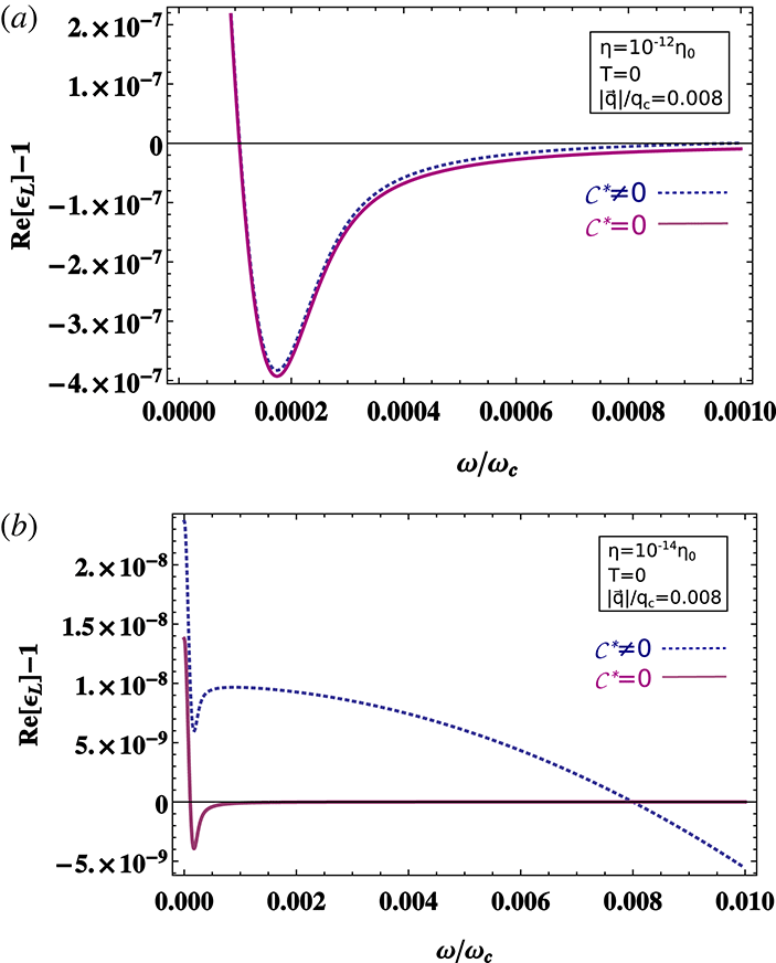
, as in non-relativistic systems. Figure 1 exhibits situations where the vacuum makes a relevant contribution to the longitudinal permittivity
 $\unicode[STIX]{x1D716}_{L}$
.
Plot of
 $(\text{Re}[\unicode[STIX]{x1D716}_{L}]-1)$
for low densities of the electron gas at
 $T=0$
. The dashed line has the vacuum contribution (
 ${\mathcal{C}}^{\ast }\neq$
 $0$
), whereas the full line only has the medium contribution (
 ${\mathcal{C}}^{\ast }=0$
). (a) Electron density
 $\unicode[STIX]{x1D702}=10^{-12}\unicode[STIX]{x1D702}_{0}$
and (b)
 $\unicode[STIX]{x1D702}=10^{-14}\unicode[STIX]{x1D702}_{0}$
, where
 $\unicode[STIX]{x1D702}_{0}\approx 1.76\times 10^{30}~\text{cm}^{-3}$
. Both the frequency and wave vector are given in units of
 $\unicode[STIX]{x1D714}_{c}=mc^{2}/\hslash$
, the Compton frequency, and
 $q_{c}=mc/\hslash$
, the Compton wave vector.

3 Real and imaginary parts of the responses
We will now explicitly compute the real and imaginary parts of the expressions for longitudinal responses both at
 $T\neq 0$
and at
 $T=0$
. For that purpose, it is convenient to define the integral in (2.7), continued to Minkowski space, as a new quantity
 ${\mathcal{D}}^{\ast }$
 $$\begin{eqnarray}{\mathcal{D}}^{\ast }={\mathcal{A}}^{\ast }-\left[1+\frac{3q^{2}}{2|\boldsymbol{q}|^{2}}\right]{\mathcal{B}}^{\ast }.\end{eqnarray}$$
Integration over angles and continuation to Minkowski space (
 $q_{4}\rightarrow \text{i}\unicode[STIX]{x1D714}-0^{+}$
) lead to
 $$\begin{eqnarray}\displaystyle & \displaystyle {\mathcal{B}}^{\ast }=\frac{-\text{e}^{2}}{\unicode[STIX]{x03C0}^{2}q^{2}}\int _{0}^{\infty }\frac{\text{d}pp^{2}n_{F}}{\unicode[STIX]{x1D700}_{p}}\left[1+\frac{4\unicode[STIX]{x1D700}_{p}^{2}+q^{2}}{8p|\boldsymbol{q}|}L_{1}+\frac{\unicode[STIX]{x1D700}_{p}\unicode[STIX]{x1D714}}{p|\boldsymbol{q}|}L_{2}\right], & \displaystyle\end{eqnarray}$$
 $$\begin{eqnarray}\displaystyle & \displaystyle {\mathcal{D}}^{\ast }=\frac{-\text{e}^{2}}{\unicode[STIX]{x03C0}^{2}q^{2}}\int _{0}^{\infty }\frac{\text{d}p\,p^{2}n_{F}}{\unicode[STIX]{x1D700}_{p}}\left[1+\frac{2m^{2}+q^{2}}{8p|\boldsymbol{q}|}L_{1}\right]. & \displaystyle\end{eqnarray}$$
The functions
 $L_{1}$
and
 $L_{2}$
are given by
 $$\begin{eqnarray}\displaystyle & \displaystyle L_{1}=\ln \left\{\frac{(\unicode[STIX]{x1D712}^{2}-by)^{2}-a^{2}x^{2}}{(\unicode[STIX]{x1D712}^{2}+by)^{2}-a^{2}x^{2}}\right\}; & \displaystyle\end{eqnarray}$$
 $$\begin{eqnarray}\displaystyle & \displaystyle L_{2}=\ln \left\{\left|\frac{\unicode[STIX]{x1D712}^{2}-by+ax}{\unicode[STIX]{x1D712}^{2}+by+ax}\right|\right\}-\frac{L_{1}}{2}, & \displaystyle\end{eqnarray}$$
where we have used dimensionless variables
 $x\equiv \unicode[STIX]{x1D700}_{p}/m$
,
 $y\equiv p/m=\sqrt{x^{2}-1}$
,
 $a\equiv \unicode[STIX]{x1D714}/2m$
,
 $b\equiv |\boldsymbol{q}|/2m$
, and
 $\unicode[STIX]{x1D712}^{2}\equiv a^{2}-b^{2}=q^{2}/4m^{2}$
.
3.1 Real parts at
 $T\neq 0$

The real parts of
 ${\mathcal{B}}^{\ast }$
and
 ${\mathcal{D}}^{\ast }$
reduce to 1-D integrals. We write them as
 $$\begin{eqnarray}\displaystyle & \displaystyle \text{Re}\,{\mathcal{B}}^{\ast }=\frac{-\text{e}^{2}}{4\unicode[STIX]{x03C0}^{2}\unicode[STIX]{x1D712}^{2}}\left(\int _{1}^{\infty }\,\text{d}xn_{F}\sqrt{x^{2}-1}+\frac{1}{4b}\int _{1}^{\infty }\,\text{d}xn_{F}[(x^{2}+\unicode[STIX]{x1D712}^{2})R_{1}+4axR_{2}]\right),\quad & \displaystyle\end{eqnarray}$$
 $$\begin{eqnarray}\displaystyle & \displaystyle \text{Re}\,{\mathcal{D}}^{\ast }=\frac{-\text{e}^{2}}{4\unicode[STIX]{x03C0}^{2}\unicode[STIX]{x1D712}^{2}}\left(\int _{1}^{\infty }\,\text{d}xn_{F}\sqrt{x^{2}-1}+\frac{1}{8b}\int _{1}^{\infty }\,\text{d}xn_{F}(1+2\unicode[STIX]{x1D712}^{2})R_{1}\right), & \displaystyle\end{eqnarray}$$
with
 $R_{1}\equiv \text{Re}\,L_{1}$
and
 $R_{2}\equiv \text{Re}\,L_{2}$
. Since
 ${\mathcal{C}}^{\ast }$
is real, we obtain
 $$\begin{eqnarray}\displaystyle & \displaystyle \text{Re}\,\unicode[STIX]{x1D716}_{L}=1+{\mathcal{C}}^{\ast }-\frac{\unicode[STIX]{x1D712}^{2}}{b^{2}}\text{Re}\,{\mathcal{B}}^{\ast }, & \displaystyle\end{eqnarray}$$
 $$\begin{eqnarray}\displaystyle & \displaystyle \text{Re}\,\unicode[STIX]{x1D708}_{L}=1+2{\mathcal{C}}^{\ast }+2\text{Re}\,{\mathcal{D}}^{\ast }+\frac{\unicode[STIX]{x1D712}^{2}}{b^{2}}\text{Re}\,{\mathcal{B}}^{\ast }. & \displaystyle\end{eqnarray}$$
The results above allow for the calculation of plasmon dispersion relations, as we will show later on.


3.2 Imaginary parts at
$T\neq 0$

From the calculations in appendix A, defining
 $\unicode[STIX]{x1D702}^{2}\equiv 1-(1/\unicode[STIX]{x1D712}^{2})$
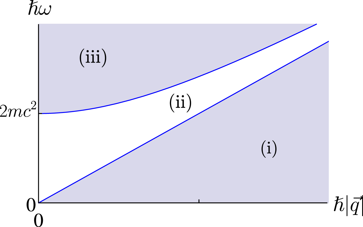
, we identify three regions in the
 $(a,b)$
plane
-
(i)
$\unicode[STIX]{x1D712}^{2}<0$
(
$\unicode[STIX]{x1D702}>1$
;
$a<b<b\unicode[STIX]{x1D702}$
):
$-a+b\unicode[STIX]{x1D702}<x<a+b\unicode[STIX]{x1D702}$
; -
(ii)
$0<\unicode[STIX]{x1D712}^{2}<1$
(
$\unicode[STIX]{x1D702}$
pure imaginary): the condition is never satisfied and
$\text{Im}\,L_{1}=0$
; -
(iii)
$\unicode[STIX]{x1D712}^{2}>1$
(
$\unicode[STIX]{x1D702}<1$
;
$a>b>b\unicode[STIX]{x1D702}$
):
$a-b\unicode[STIX]{x1D702}<x<a+b\unicode[STIX]{x1D702}$
.



They are shown in figure 2. For the longitudinal responses, we have
 $$\begin{eqnarray}\displaystyle & \displaystyle \text{Im}\,\unicode[STIX]{x1D716}_{L}=-\frac{\text{sign}(\unicode[STIX]{x1D712}^{2})\text{e}^{2}}{16\unicode[STIX]{x03C0}b^{3}}\int _{x_{l}}^{a+b\unicode[STIX]{x1D702}}\,\text{d}xn_{F}[(x-a)^{2}-b^{2}] & \displaystyle\end{eqnarray}$$
 $$\begin{eqnarray}\displaystyle & \displaystyle \text{Im}\,\unicode[STIX]{x1D708}_{L}=\frac{\text{sign}(\unicode[STIX]{x1D712}^{2})\text{e}^{2}}{16\unicode[STIX]{x03C0}b\unicode[STIX]{x1D712}^{2}}\int _{x_{l}}^{a+b\unicode[STIX]{x1D702}}\,\text{d}xn_{F}(1+2\unicode[STIX]{x1D712}^{2})-\text{Im}\,\unicode[STIX]{x1D716}_{L}. & \displaystyle\end{eqnarray}$$
 $\text{Im}\,\unicode[STIX]{x1D708}_{L}$
and
 $\text{Im}\,\unicode[STIX]{x1D716}_{L}$
vanish in region (ii) of the
 $(a,b)$
plane. In region (i)
 $x_{l}=-a+b\unicode[STIX]{x1D702}$
and in region (iii)
 $x_{l}=a-b\unicode[STIX]{x1D702}$
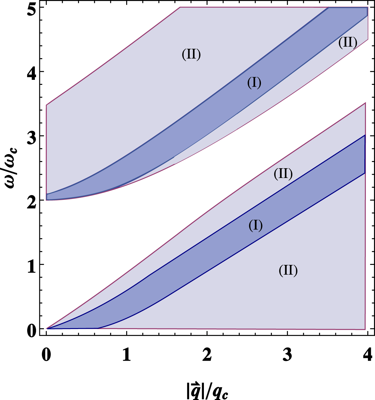
. Using the expressions for the imaginary parts in regions (i) and (iii), we may see how their values evolve from
 $T=0$
to non-zero temperatures. This is shown in figure 3. One should note that the appearance of non-zero imaginary parts is associated with the creation of electron–hole (lower energies) or electron–positron (higher energies) pairs.
Evolution with temperature of the regions of the
 $(a,b)\sim (\hbar \unicode[STIX]{x1D714},\hbar |\boldsymbol{q}|)$
plane with non-vanishing imaginary parts. As
 $\tilde{\unicode[STIX]{x1D6FD}}$
decreases, the two
 $T=0$
regions (labelled
 $\text{I}$
) expand. For a value of
 $\tilde{\unicode[STIX]{x1D6FD}}=10^{3}$
, imaginary parts appear in all regions labelled
 $\text{I}$
and
 $\text{II}$
. Eventually, as
 $T\rightarrow \infty$
, only the unshaded region of figure 2 will have vanishing imaginary parts.

We have thus derived electromagnetic responses as functions of
 $a$
,
 $b$
,
 $T/m$
and
 $\unicode[STIX]{x1D709}/m$
, the two latter dependences from coming from the Fermi–Dirac distribution function.
3.3 Imaginary parts at
$T=0$

At
 $T=0$
,
 $n_{F}(x)\rightarrow \unicode[STIX]{x1D6E9}(x_{F}-x)$
, with
 $x_{F}\equiv \unicode[STIX]{x1D700}_{F}/m=\unicode[STIX]{x1D709}/m$
and
 $y_{F}=(1/m)\sqrt{\unicode[STIX]{x1D700}_{F}^{2}-m^{2}}=p_{F}/m$
. We may then analytically perform the integrals for both the imaginary and real parts of the response functions. Additional restrictions come into play because of the integration limit
 $x_{F}$
imposed by the function
 $\unicode[STIX]{x1D6E9}(x_{F}-x)$
.
From the calculations in appendix A, we identify four regions in the
 $(a,b)$
plane where the longitudinal responses will have different values. We use
 $[f(x)]_{x_{l}}^{x_{u}}\equiv f(x_{u})-f(x_{l})$
and refer the reader to the appendix B for the calculation of
 $b_{\pm }$
,
 $\bar{b}_{\pm }$
,
 $b_{\pm }^{\prime }$
and
 $\bar{b}_{\pm }^{\prime }$
. The regions are
(A) for
 $0<a<(x_{F}-1)/2$
and
 $(x_{F}+1)/2<a<x_{F}$
,
 $\bar{b}_{-}<b<\bar{b}_{+}$
,
 $x_{l}=-a+b\unicode[STIX]{x1D702}$
,
 $x_{u}=a+b\unicode[STIX]{x1D702}$
,
 $$\begin{eqnarray}\left.\begin{array}{@{}c@{}}\displaystyle \text{Im}\,\unicode[STIX]{x1D716}_{L}=\frac{\text{e}^{2}}{48\unicode[STIX]{x03C0}b^{3}}[(x-a)^{3}-3b^{2}x]_{-a+b\unicode[STIX]{x1D702}}^{a+b\unicode[STIX]{x1D702}},\\ \displaystyle \text{Im}\,\unicode[STIX]{x1D708}_{L}=-\frac{\text{e}^{2}}{16\unicode[STIX]{x03C0}b\unicode[STIX]{x1D712}^{2}}[2a(1+2\unicode[STIX]{x1D712}^{2})]-\text{Im}\,\unicode[STIX]{x1D716}_{L};\end{array}\right\}\end{eqnarray}$$
(B) for
 $(x_{F}-1)/2<a<(x_{F}+1)/2$
and
 $a>x_{F}$
,
 $b_{-}<b<b_{+}$
,
 $x_{l}=-a+b\unicode[STIX]{x1D702}$
,
 $x_{u}=x_{F}$
,
 $$\begin{eqnarray}\left.\begin{array}{@{}c@{}}\displaystyle \text{Im}\,\unicode[STIX]{x1D716}_{L}=\frac{\text{e}^{2}}{48\unicode[STIX]{x03C0}b^{3}}[(x-a)^{3}-3b^{2}x]_{-a+b\unicode[STIX]{x1D702}}^{x_{F}},\\ \displaystyle \text{Im}\,\unicode[STIX]{x1D708}_{L}=-\frac{\text{e}^{2}}{16\unicode[STIX]{x03C0}b\unicode[STIX]{x1D712}^{2}}[(x_{F}+a-b\unicode[STIX]{x1D702})(1+2\unicode[STIX]{x1D712}^{2})]-\text{Im}\,\unicode[STIX]{x1D716}_{L}.\end{array}\right\}\end{eqnarray}$$
Outside regions (A) and (B), for
 $\unicode[STIX]{x1D712}^{2}<0$
the imaginary parts of
 $\unicode[STIX]{x1D716}_{L}$
and
 $\unicode[STIX]{x1D708}_{L}$
vanish.
(C) for
 $0<a<(x_{F}-1)/2$
and
 $(x_{F}+1)/2<a<x_{F}$
,
 $\bar{b}_{-}^{\prime }<b<\bar{b}_{+}^{\prime }$
,
 $x_{l}=a-b\unicode[STIX]{x1D702}$
,
 $x_{u}=a+b\unicode[STIX]{x1D702}$
,
 $$\begin{eqnarray}\left.\begin{array}{@{}c@{}}\displaystyle \text{Im}\,\unicode[STIX]{x1D716}_{L}=-\frac{\text{e}^{2}}{48\unicode[STIX]{x03C0}b^{3}}[(x-a)^{3}-3b^{2}x]_{a-b\unicode[STIX]{x1D702}}^{a+b\unicode[STIX]{x1D702}},\\ \displaystyle \text{Im}\,\unicode[STIX]{x1D708}_{L}=\frac{\text{e}^{2}}{16\unicode[STIX]{x03C0}b\unicode[STIX]{x1D712}^{2}}[2b\unicode[STIX]{x1D702}(1+2\unicode[STIX]{x1D712}^{2})]-\text{Im}\,\unicode[STIX]{x1D716}_{L};\end{array}\right\}\end{eqnarray}$$
(D) for
 $(x_{F}-1)/2<a<(x_{F}+1)/2$
and
 $a>x_{F}$
,
 $b_{-}^{\prime }<b<b_{+}^{\prime }$
,
 $x_{l}=a-b\unicode[STIX]{x1D702}$
,
 $x_{u}=x_{F}$
,
 $$\begin{eqnarray}\left.\begin{array}{@{}c@{}}\displaystyle \text{Im}\,\unicode[STIX]{x1D716}_{L}=-\frac{\text{e}^{2}}{48\unicode[STIX]{x03C0}b^{3}}[(x-a)^{3}-3b^{2}x]_{a-b\unicode[STIX]{x1D702}}^{x_{F}},\\ \displaystyle \text{Im}\,\unicode[STIX]{x1D708}_{L}=\frac{\text{e}^{2}}{16\unicode[STIX]{x03C0}b\unicode[STIX]{x1D712}^{2}}[(x_{F}-a+b\unicode[STIX]{x1D702})(1+2\unicode[STIX]{x1D712}^{2})]-\text{Im}\,\unicode[STIX]{x1D716}_{L}.\end{array}\right\}\end{eqnarray}$$
Outside regions (C) and (D), for
 $\unicode[STIX]{x1D712}^{2}>1$
the imaginary parts of
 $\unicode[STIX]{x1D716}_{L}$
and
 $\unicode[STIX]{x1D708}_{L}$
vanish.
Finally, in case (ii),
 $0<\unicode[STIX]{x1D712}^{2}<1$
, one has
 $\text{Im}\,\unicode[STIX]{x1D716}_{L}=\text{Im}\,\unicode[STIX]{x1D708}_{L}=0$
.
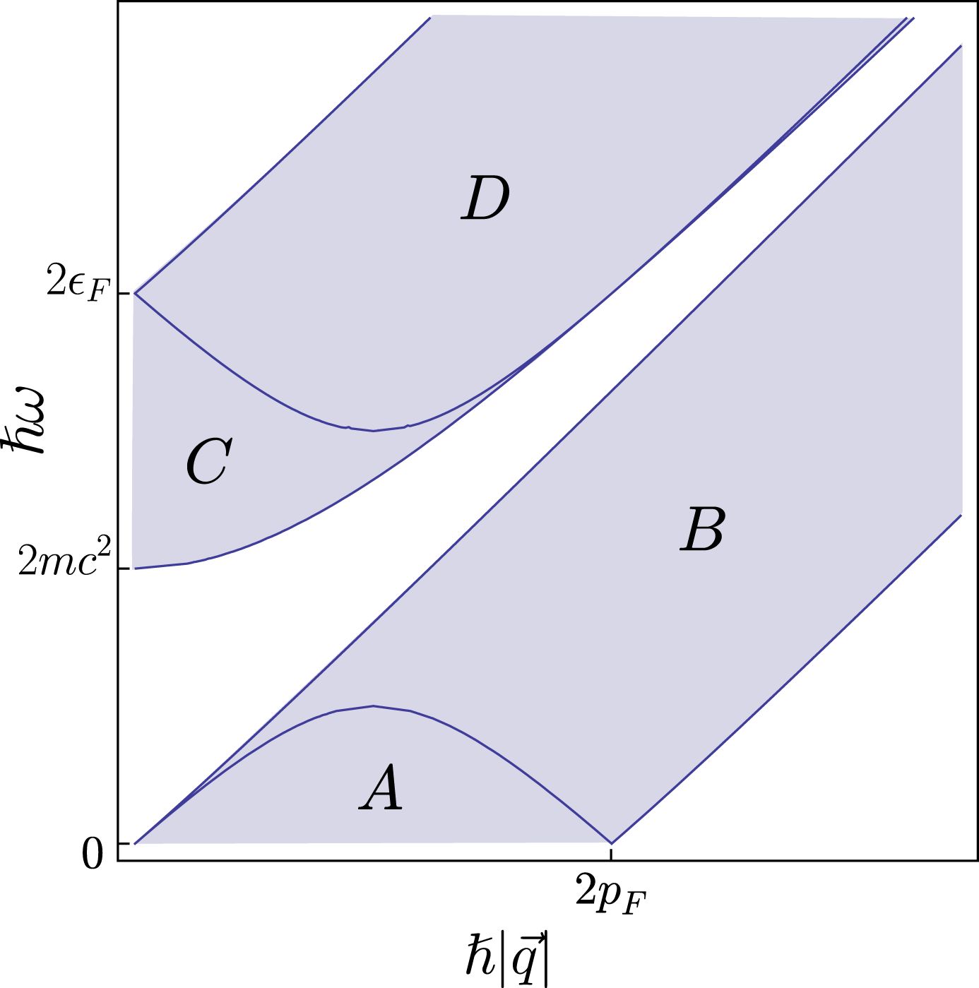
The various regions of the (a,b) plane that correspond to the different expressions discussed above are depicted in figure 4.
Regions in the
 $(a,b)\sim (\hbar \unicode[STIX]{x1D714},\hbar |\boldsymbol{q}|)$
plane where the imaginary parts are non-vanishing for
 $T=0$
. The limits of regions A, B, C, D and the values of the longitudinal responses in each of them are shown in § 3.3.

3.4 Real parts at
$T=0$

For the real parts at
 $T=0$
, we replace
 $n_{F}$
with
 $\unicode[STIX]{x1D6E9}(x_{F}-x)$
in (3.6) and (3.7). The calculations detailed in appendices C and D lead to
 $$\begin{eqnarray}\displaystyle & \displaystyle \text{Re}\,{\mathcal{B}}^{\ast }=\frac{-\text{e}^{2}}{4\unicode[STIX]{x03C0}^{2}\unicode[STIX]{x1D712}^{2}}[X_{B}+Y_{B}+Z_{B}], & \displaystyle\end{eqnarray}$$
 $$\begin{eqnarray}\displaystyle & \displaystyle \text{Re}\,{\mathcal{D}}^{\ast }=\frac{-\text{e}^{2}}{4\unicode[STIX]{x03C0}^{2}\unicode[STIX]{x1D712}^{2}}[X_{D}+Y_{D}+Z_{D}], & \displaystyle\end{eqnarray}$$
where
 $X_{B}$
,
 $X_{D}$
,
 $Y_{B}$
and
 $Y_{D}$
are given by (
 $R_{i}=\text{Re}\,L_{i}$
; (3.4), (3.5))
 $$\begin{eqnarray}\displaystyle & \displaystyle X_{B}=\frac{x_{F}}{12b}[(x_{F}^{2}+3\unicode[STIX]{x1D712}^{2})R_{1}(x_{F})+6ax_{F}R_{2}(x_{F})], & \displaystyle\end{eqnarray}$$
 $$\begin{eqnarray}\displaystyle & \displaystyle X_{D}=\frac{x_{F}}{8b}(1+2\unicode[STIX]{x1D712}^{2})R_{1}(x_{F}), & \displaystyle\end{eqnarray}$$
 $$\begin{eqnarray}\displaystyle & \displaystyle Y_{B}={\textstyle \frac{2}{3}}[x_{F}y_{F}-b^{2}\ln (x_{F}+y_{F})], & \displaystyle\end{eqnarray}$$
 $$\begin{eqnarray}\displaystyle & \displaystyle Y_{D}={\textstyle \frac{1}{2}}[x_{F}y_{F}+2\unicode[STIX]{x1D712}^{2}\ln (x_{F}+y_{F})], & \displaystyle\end{eqnarray}$$
whereas
 $Z_{B}$
and
 $Z_{D}$
are given by
 $$\begin{eqnarray}Z_{B,D}=C_{B,D}[(M_{B,D}+N_{B,D})\mathfrak{I}_{0}-N_{B,D}\mathfrak{I}_{2}].\end{eqnarray}$$
 $C_{B,D}(a,b)$
,
 $M_{B,D}(a,b)$
,
 $N_{B,D}(a,b)$
and the integrals
 $\mathfrak{I}_{0}(a,b,x_{F})$
and
 $\mathfrak{I}_{2}(a,b,x_{F})$
are defined and calculated in the appendix D.
The longitudinal responses (2.19) and (2.20) are given by
 $$\begin{eqnarray}\displaystyle & \displaystyle \text{Re}\,\unicode[STIX]{x1D716}_{L}=1+{\mathcal{C}}^{\ast }+\frac{\text{e}^{2}}{4\unicode[STIX]{x03C0}^{2}b^{2}}[X_{B}+Y_{B}+Z_{B}], & \displaystyle\end{eqnarray}$$
 $$\begin{eqnarray}\displaystyle & \displaystyle \text{Re}\,\unicode[STIX]{x1D708}_{L}=1+2{\mathcal{C}}^{\ast }-\frac{\text{e}^{2}}{2\unicode[STIX]{x03C0}^{2}\unicode[STIX]{x1D712}^{2}}[X_{D}+Y_{D}+Z_{D}]-\frac{\text{e}^{2}}{4\unicode[STIX]{x03C0}^{2}b^{2}}[X_{B}+Y_{B}+Z_{B}]. & \displaystyle\end{eqnarray}$$
4 Plasmon excitations
As mentioned in the introduction, electromagnetic responses may be used to obtain the dispersion relation for plasmon modes that propagate when external electromagnetic fields induce resonant charge density collective oscillations in the electron gas. The dispersion relation for longitudinal electric plasmons, for instance, is obtained from the well-known condition
 $\unicode[STIX]{x1D716}_{L}=0$
(Abrikosov & Dzyaloshinski Reference Abrikosov, Gorkov and Dzyaloshinski1975; Sturm & Oliveira Reference Sturm and Oliveira1980, Reference Sturm and Oliveira1981; Sturm Reference Sturm1982; Fetter & Walecka Reference Fetter and Walecka2012). As an application of our formulae, we will use our expressions for
 $\text{Re}\,\unicode[STIX]{x1D716}_{L}$
and
 $\text{Im}\,\unicode[STIX]{x1D716}_{L}$
to obtain it.
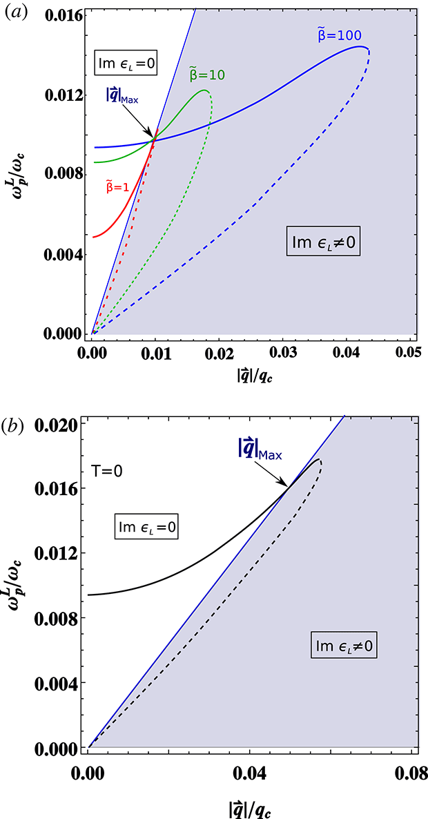
The solutions to
 $\text{Re}\,\unicode[STIX]{x1D716}_{L}=0$
are plotted in figure 5(a,b), for the case
 $T\neq 0$
and
 $T=0$
. Since we must have
 $\unicode[STIX]{x1D716}_{L}=0$
, the full curve in the figure is the physical one, because most of it lies in the unshaded region, where we also have
 $\text{Im}\,\unicode[STIX]{x1D716}_{L}=0$
. The dashed curve lies completely in the region where there is an imaginary part, so that it never satisfies
 $\unicode[STIX]{x1D716}_{L}=0$
.
The shaded region in figure 5(b) is the same as the lower region of figure 4, where
 $\text{Im}\,\unicode[STIX]{x1D716}_{L}\neq 0$
. The dashed curve is fully within that region and thus a decaying mode, whereas the full curve lies mostly in the region where
 $\text{Im}\,\unicode[STIX]{x1D716}_{L}=0$
. Thus, it describes a plasmon mode. As the curve enters the region where there is an imaginary part, the plasmon mode becomes unstable to the decay into electron–hole pairs, just as in the non-relativistic case.
Analytic results at
 $T=0$
and numerical results at
 $T\neq 0$
may be used to compute decay constants and dispersion relations for both longitudinal and transverse plasmons. A complete discussion of the modes that propagate in the relativistic electron gas will appear elsewhere (Reis & de Carvalho Reference Reis, Reyes-Gómez and de Carvalho2017).
One may use our expressions to confirm that, for long wavelengths and below their plasmon frequencies, both
 $\unicode[STIX]{x1D716}_{L}$
and
 $\unicode[STIX]{x1D708}_{L}$
will be simultaneously negative, a behaviour previously thought to occur only in artificially nanoengineered materials. Our calculations show that this behaviour is natural in relativistic systems, where magnetic effects are not suppressed by
 $v/c$
, unlike what happens in the non-relativistic limit, where
 $\unicode[STIX]{x1D708}_{L}\sim 1$
.
Upper (
 $\unicode[STIX]{x1D714}_{p}^{L}$
plasmon frequency) and lower frequency zeroes of
 $\unicode[STIX]{x1D716}_{L}$
(Solid and dashed lines, respectively) as functions of the
 $|\boldsymbol{q}|$
wave vector. Calculations were performed for (a)
 $\tilde{\unicode[STIX]{x1D6FD}}=100$
,
 $\tilde{\unicode[STIX]{x1D6FD}}=10$
,
 $\tilde{\unicode[STIX]{x1D6FD}}=1$
and (b)
 $\tilde{\unicode[STIX]{x1D6FD}}\rightarrow \infty (T=0)$
by taking the density electron gas
 $\unicode[STIX]{x1D702}=10^{-2}\unicode[STIX]{x1D702}_{0}$
, where
 $\unicode[STIX]{x1D702}_{0}\approx 1.76\times 10^{30}~\text{cm}^{-3}$
. The shaded area corresponds to the region where electron–hole excitations occur. Note the maximum value of the wave vector
 $(|\boldsymbol{q}|_{max})$
beyond which the longitudinal plasmon decays into electron-hole pairs.

5 Conclusions
The unified treatment provided by QED at finite temperature and density allows one to relate the electromagnetic responses of the relativistic electron gas to the polarization tensor of QED which incorporates vacuum and medium effects. This is a first-principle calculation that opens up interesting possibilities, since the computation can be extended to other systems and to different dimensions.
We have thus used QED to compute the real and imaginary parts of both the electric and magnetic longitudinal responses of the relativistic electron gas. One may show that the non-relativistic limit of the present theoretical results for the dielectric response coincide with the celebrated Lindhard dielectric function (Lindhard Reference Lindhard1954). For
 $T=0$
, we obtain analytic expressions that coincide with those existing in the literature if we neglect the vacuum contributions.
The appearance of non-zero imaginary parts indicates that the system is unstable to the decay into electron–hole (lower energies) or electron–positron (higher energies) pairs (Tsai & Erber Reference Tsai and Erber1974; Pulsifer & Kalman Reference Pulsifer and Kalman1992). The former is well known to occur in the non-relativistic limit. Furthermore, the explicit expressions for longitudinal electric and magnetic responses allow for the calculation of dispersion relations for plasmons.
We hope that experimental data from synchrotron beams or observational data from astrophysical scenarios will allow us to test our predictions, just as we have done in Condensed Matter systems (Reyes-Gómez & de Carvalho Reference Reyes-Gómez, Oliveira and de Carvalho2016).
Acknowledgements
The authors wish to thank L. E. Oliveira for many fruitful discussions, for a critical reading of the manuscript, and for his warm hospitality at the Institute of Physics of the Universidade Estadual de Campinas, where part of this work was done. Thanks are also due to E. Reyes-Gómez for discussions and help with the figures, and to CAPES, CNPq and FAPESP for financial support.
Appendix A. Imaginary parts at
$T\neq 0$

The vacuum contribution does not have an imaginary part. On the other hand, imaginary parts for
 ${\mathcal{B}}^{\ast }$
and
 ${\mathcal{D}}^{\ast }$
will appear whenever the argument in
 $L_{1}$
becomes negative (note that
 $\text{Im}\,L_{2}=-\text{Im}\,L_{1}/2$
). For that to occur, the product of the numerator
 $\mathfrak{N}$
times the denominator
 $\mathfrak{D}$
of the argument must satisfy,
 $$\begin{eqnarray}\mathfrak{N}\mathfrak{D}=[(\unicode[STIX]{x1D712}^{2}-by)^{2}-a^{2}x^{2}][(\unicode[STIX]{x1D712}^{2}+by)^{2}-a^{2}x^{2}]<0.\end{eqnarray}$$
The roots of the related biquadratic equation in
 $x$
(
 ${\geqslant}0$
) are
 $x_{\pm }=a\pm b\unicode[STIX]{x1D702}$
, where
 $\unicode[STIX]{x1D702}^{2}\equiv 1-(1/\unicode[STIX]{x1D712}^{2})$
, leading to the condition
 $(a-b\unicode[STIX]{x1D702})^{2}<x^{2}<(a+b\unicode[STIX]{x1D702})^{2}$
.
Three cases have to be considered:
-
(i)
$\unicode[STIX]{x1D712}^{2}<0$
(
$\unicode[STIX]{x1D702}>1$
;
$a<b<b\unicode[STIX]{x1D702}$
):
$-a+b\unicode[STIX]{x1D702}<x<a+b\unicode[STIX]{x1D702}$
; -
(ii)
$0<\unicode[STIX]{x1D712}^{2}<1$
(
$\unicode[STIX]{x1D702}$
pure imaginary): the condition is never satisfied and
$\text{Im}\,L_{1}=0$
; -
(iii)
$\unicode[STIX]{x1D712}^{2}>1$
(
$\unicode[STIX]{x1D702}<1$
;
$a>b>b\unicode[STIX]{x1D702}$
):
$a-b\unicode[STIX]{x1D702}<x<a+b\unicode[STIX]{x1D702}$
.



The difference between numerator
 $\mathfrak{N}$
and denominator
 $\mathfrak{D}$
is given by
 $-\unicode[STIX]{x1D712}^{2}by$
. For case (i), this implies
 $\mathfrak{N}>0$
,
 $\mathfrak{D}<0$
whereas for case (iii)
 $\mathfrak{N}<0$
,
 $\mathfrak{D}>0$
. For case (ii),
 $0<\unicode[STIX]{x1D712}^{2}<1$
, corresponding to the same sign for
 $\mathfrak{N}$
and
 $\mathfrak{D}$
,
 $\text{Im}\,{\mathcal{B}}^{\ast }=\text{Im}\,{\mathcal{D}}^{\ast }=0$
.
For cases (i) and (iii), we take
 $\text{Im}\,L_{1}=\text{sign}(\mathfrak{N})\unicode[STIX]{x03C0}$
. The choice of sign corresponds to the continuation
 $q_{4}\rightarrow \text{i}\unicode[STIX]{x1D714}-0^{+}$
. Therefore
 $$\begin{eqnarray}\displaystyle & \displaystyle \text{Im}\,{\mathcal{B}}^{\ast }=\frac{\text{sign}(\unicode[STIX]{x1D712}^{2})\text{e}^{2}}{16\unicode[STIX]{x03C0}b\unicode[STIX]{x1D712}^{2}}\int _{x_{l}}^{a+b\unicode[STIX]{x1D702}}\,\text{d}xn_{F}[(x-a)^{2}-b^{2}] & \displaystyle\end{eqnarray}$$
 $$\begin{eqnarray}\displaystyle & \displaystyle \text{Im}\,{\mathcal{D}}^{\ast }=\frac{\text{sign}(\unicode[STIX]{x1D712}^{2})\text{e}^{2}}{32\unicode[STIX]{x03C0}b\unicode[STIX]{x1D712}^{2}}\int _{x_{l}}^{a+b\unicode[STIX]{x1D702}}\,\text{d}xn_{F}(1+2\unicode[STIX]{x1D712}^{2}). & \displaystyle\end{eqnarray}$$
For case (i),
 $\unicode[STIX]{x1D712}^{2}<0$
,
 $\mathfrak{N}>0$
, and
 $x_{l}=-a+b\unicode[STIX]{x1D702}$
whereas for case (iii),
 $\unicode[STIX]{x1D712}^{2}>1$
,
 $\mathfrak{N}<0$
, and
 $x_{l}=a-b\unicode[STIX]{x1D702}$
. It is easy to show that
 $-a+b\unicode[STIX]{x1D702}>1$
in case (i) and
 $a-b\unicode[STIX]{x1D702}>1$
in case (iii). Thus, imaginary parts may appear for both
 ${\mathcal{B}}^{\ast }$
and
 ${\mathcal{D}}^{\ast }$
in the regions
 $\unicode[STIX]{x1D712}^{2}<0$
and
 $\unicode[STIX]{x1D712}^{2}>1$
of the
 $(a,b)$
plane, but they vanish for
 $0<\unicode[STIX]{x1D712}^{2}<1$
.
Appendix B. Imaginary parts at
$T=0$

Again, the vacuum contribution does not have an imaginary part. We then refer to the three cases described in § 3.2, which correspond to different regions in the
 $(a,b)$
plane.
In case (i),
 $\unicode[STIX]{x1D712}^{2}<0$
,
 $\unicode[STIX]{x1D702}>1$
,
 $a<b<b\unicode[STIX]{x1D702}$
, the lower integration limit of (A 2), (A 3) is
 $x_{l}=-a+b\unicode[STIX]{x1D702}$
whereas the upper one is
 $x_{u}=a+b\unicode[STIX]{x1D702}$
. For a non-vanishing result, we need
 $x_{l}=-a+b\unicode[STIX]{x1D702}<x_{F}$
. This will occur if
 $b_{-}<b<b_{+}$
, where
 $$\begin{eqnarray}b_{\pm }=\pm \frac{y_{F}}{2}+\sqrt{\frac{y_{F}^{2}}{4}+a(x_{F}+a)}.\end{eqnarray}$$
Depending on whether
 $x_{u}<x_{F}$
or
 $x_{u}>x_{F}$
, results for the imaginary part will differ. For
 $x_{u}=a+b\unicode[STIX]{x1D702}<x_{F}$
, one needs
 $a<x_{F}$
and
 $$\begin{eqnarray}\displaystyle & \displaystyle b^{2}-y_{F}b+a(x_{F}-a)<0, & \displaystyle\end{eqnarray}$$
 $$\begin{eqnarray}\displaystyle & \displaystyle b^{2}+y_{F}b+a(x_{F}-a)>0. & \displaystyle\end{eqnarray}$$
To satisfy (B 2), the argument of the square-root appearing in the roots of the associated equation has to be positive, so that
 $0<a<(x_{F}-1)/2$
and
 $(x_{F}+1)/2<a<x_{F}$
. Then, (B 3) will always be satisfied whereas (B 2) implies
 $\bar{b}_{-}<b<\bar{b}_{+}$
, where
 $$\begin{eqnarray}\bar{b}_{\pm }=\frac{y_{F}}{2}\pm \sqrt{\frac{y_{F}^{2}}{4}-a(x_{F}-a)}.\end{eqnarray}$$
As a result, the integrals in (A 2) and (A 3), with the definition
 $[f(x)]_{x_{l}}^{x_{u}}\equiv f(x_{u})-f(x_{l})$
, define regions (A) and (B) in § 3.3.
In case (iii) [
 $\unicode[STIX]{x1D712}^{2}>1$
,
 $\unicode[STIX]{x1D702}<1$
(
 $a>b>b\unicode[STIX]{x1D702}$
)], the lower integration limit of (A 2), (A 3) is
 $x_{l}=a-b\unicode[STIX]{x1D702}$
whereas the upper one is
 $x_{u}=a+b\unicode[STIX]{x1D702}$
. For a non-vanishing result,
 $x_{l}=a-b\unicode[STIX]{x1D702}<x_{F}$
. This will always occur if
 $a<x_{F}$
whereas for
 $a>x_{F}$
,
 $b_{-}^{\prime }<b<b_{+}^{\prime }$
, where
 $$\begin{eqnarray}b_{\pm }^{\prime }=\pm \frac{y_{F}}{2}+\sqrt{\frac{y_{F}^{2}}{4}-a(x_{F}-a)}.\end{eqnarray}$$
Again, depending on whether
 $x_{u}<x_{F}$
or
 $x_{u}>x_{F}$
, results for the imaginary part will differ. For
 $x_{u}=a+b\unicode[STIX]{x1D702}<x_{F}$
,
 $a<x_{F}$
and
 $$\begin{eqnarray}\displaystyle & \displaystyle b^{2}-y_{F}b+a(x_{F}-a)>0, & \displaystyle\end{eqnarray}$$
 $$\begin{eqnarray}\displaystyle & \displaystyle b^{2}+y_{F}b+a(x_{F}-a)>0. & \displaystyle\end{eqnarray}$$
To satisfy (B 6), the argument of the square-root appearing in the roots of the associated equation has to be positive, so that
 $0<a<(x_{F}-1)/2$
and
 $(x_{F}+1)/2<a<x_{F}$
. Then, (B 7) will always be satisfied whereas (B 6) implies
 $\bar{b}_{-}^{\prime }<b<\bar{b}_{+}^{\prime }$
, with
 $$\begin{eqnarray}\bar{b}_{\pm }^{\prime }=\frac{y_{F}}{2}\pm \sqrt{\frac{y_{F}^{2}}{4}-a(x_{F}-a)}.\end{eqnarray}$$
We may then define regions (C) and (D) in § 3.3.
Appendix C. Real parts at
$T=0$

The first integral in expressions (3.6) and (3.7) is simply
 $$\begin{eqnarray}{\textstyle \frac{1}{2}}[x_{F}y_{F}-\ln (x_{F}+y_{F})],\end{eqnarray}$$
whereas the last ones may be integrated by parts, using
 $R_{1}(1)=R_{2}(1)=0$
, to yield
 $$\begin{eqnarray}\frac{x_{F}}{12b}[(x_{F}^{2}+3\unicode[STIX]{x1D712}^{2})R_{1}(x_{F})+6ax_{F}R_{2}(x_{F})]-\frac{1}{12b}\int _{1}^{x_{F}}\,\text{d}x[(x^{3}+3\unicode[STIX]{x1D712}^{2}x)R_{1}^{\prime }+6ax^{2}R_{2}^{\prime }],\end{eqnarray}$$
for (3.6), and
 $$\begin{eqnarray}\frac{x_{F}}{8b}(1+2\unicode[STIX]{x1D712}^{2})R_{1}(x_{F})-\frac{1}{8b}\int _{1}^{x_{F}}\,\text{d}x(1+2\unicode[STIX]{x1D712}^{2})xR_{1}^{\prime },\end{eqnarray}$$
for (3.7). It is convenient to introduce
 $$\begin{eqnarray}L_{\pm }(x)\equiv \ln \left(\frac{|\pm ax+by+\unicode[STIX]{x1D712}^{2}|}{|\pm ax-by+\unicode[STIX]{x1D712}^{2}|}\right),\end{eqnarray}$$
so that
 $R_{1}=-(L_{+}+L_{-})$
,
 $R_{2}=-(L_{+}+L_{-})/2$
. Taking derivatives, dividing out the resulting polynomials and adding the
 $\pm$
contributions leads to
 $$\begin{eqnarray}\frac{x_{F}}{12b}[(x_{F}^{2}+3\unicode[STIX]{x1D712}^{2})R_{1}(x_{F})+6ax_{F}R_{2}(x_{F})]+\frac{1}{6}[x_{F}y_{F}+(3-4b^{2})\ln (x_{F}+y_{F})]+Z_{B},\end{eqnarray}$$
for (3.6) and
 $$\begin{eqnarray}\frac{x_{F}}{8b}(1+2\unicode[STIX]{x1D712}^{2})R_{1}(x_{F})+\frac{1}{2}(1+2\unicode[STIX]{x1D712}^{2})\ln (x_{F}+y_{F})+Z_{D},\end{eqnarray}$$
for (3.7), with
 $Z_{B}$
and
 $Z_{D}$
defined and calculated in appendix D.
Appendix D. Definition and calculation of
$Z_{B}$
and
$Z_{D}$


The explicit expressions of
 $Z_{B,D}$
are
 $$\begin{eqnarray}Z_{B,D}=C_{B,D}\int _{1}^{x_{F}}\frac{\text{d}x}{\sqrt{x^{2}-1}}\frac{M_{B,D}x^{2}+N_{B,D}}{(x^{2}+\unicode[STIX]{x1D701}^{2})^{2}-4a^{2}x^{2}},\end{eqnarray}$$
where
 $\unicode[STIX]{x1D701}^{2}\equiv a^{2}-\unicode[STIX]{x1D702}^{2}b^{2}$
,
 $C_{B}=1/3$
and
 $C_{D}=(1+2\unicode[STIX]{x1D712}^{2})/2$
. The expressions for
 $M_{B,D}$
and
 $N_{B,D}$
depend solely on
 $a$
and
 $b$
,
 $$\begin{eqnarray}\left.\begin{array}{@{}c@{}}\displaystyle M_{B}=-2a^{2}(1+4b^{2})-[1-2b^{2}-2a^{2}(2-\unicode[STIX]{x1D702}^{2})]\unicode[STIX]{x1D701}^{2},\\ \displaystyle N_{B}=-\unicode[STIX]{x1D701}^{4}(1-2b^{2}),\\ \displaystyle M_{D}=2a^{2}(1+\unicode[STIX]{x1D702}^{2})-\unicode[STIX]{x1D701}^{2},\\ \displaystyle N_{D}=-\unicode[STIX]{x1D701}^{4}.\end{array}\right\}\end{eqnarray}$$
Defining
 $t=\sqrt{(x^{2}-1)/x^{2}}=y/x$
, (D 1) reduces to
 $$\begin{eqnarray}Z_{B,D}=C_{B,D}[(M_{B,D}+N_{B,D})\mathfrak{I}_{0}-N_{B,D}\mathfrak{I}_{2}],\end{eqnarray}$$
where
 $\mathfrak{I}_{j}$
is
 $$\begin{eqnarray}\mathfrak{I}_{j}=\int _{0}^{t_{F}}\frac{\text{d}tt^{j}}{\mathfrak{C}t^{4}+\mathfrak{B}t^{2}+\mathfrak{A}},\end{eqnarray}$$
and the coefficients are
 $\mathfrak{C}=\unicode[STIX]{x1D701}^{4}$
,
 $\mathfrak{B}=-2[\unicode[STIX]{x1D701}^{2}(\unicode[STIX]{x1D701}^{2}+1)-2a^{2}]$
, and
 $\mathfrak{A}=(\unicode[STIX]{x1D701}^{2}+1)^{2}-4a^{2}$
. There are two cases to be considered, depending on the roots of the biquadratic equation
 $\mathfrak{C}t^{4}+\mathfrak{B}t^{2}+\mathfrak{A}=0$
:
(i) For
 $\unicode[STIX]{x1D702}^{2}>0$
, the roots are real
 $$\begin{eqnarray}t_{\pm }^{2}=\frac{\unicode[STIX]{x1D701}^{2}(\unicode[STIX]{x1D701}^{2}+1)-2a^{2}\pm 2ab|\unicode[STIX]{x1D702}|}{\unicode[STIX]{x1D701}^{4}},\end{eqnarray}$$
so that the integrals become
 $$\begin{eqnarray}\mathfrak{I}_{j}=\frac{1}{4ab|\unicode[STIX]{x1D702}|}\left[t_{+}^{\,j}\int _{0}^{t_{F}}\frac{\text{d}t}{t^{2}-t_{+}^{2}}-t_{-}^{\,j}\int _{0}^{t_{F}}\frac{\text{d}t}{t^{2}-t_{-}^{2}}\right].\end{eqnarray}$$
One may show that
 $t_{\pm }^{2}>0$
, therefore
 $$\begin{eqnarray}\int _{0}^{t_{F}}\frac{\text{d}t}{t^{2}-t_{\pm }^{2}}=\frac{1}{2t_{\pm }}\ln \left|\frac{t_{F}-t_{\pm }}{t_{F}+t_{\pm }}\right|,\end{eqnarray}$$
where, from (D 5), we may write
 $t_{\pm }=(y_{\pm }/|x_{\pm }|)$
, with
 $x_{\pm }=a\pm b\unicode[STIX]{x1D702}$
and
 $y_{\pm }=\sqrt{x_{\pm }^{2}-1}$
. Then,
 $$\begin{eqnarray}\displaystyle & \displaystyle \mathfrak{I}_{0}=\frac{1}{4ab|\unicode[STIX]{x1D702}|}\left[\frac{1}{2t_{+}}\ln \left|\frac{t_{F}-t_{+}}{t_{F}+t_{+}}\right|-(t_{+}\rightarrow t_{-})\right], & \displaystyle\end{eqnarray}$$
 $$\begin{eqnarray}\displaystyle & \displaystyle \mathfrak{I}_{2}=\frac{1}{4ab|\unicode[STIX]{x1D702}|}\left[\frac{t_{+}}{2}\ln \left|\frac{t_{F}-t_{+}}{t_{F}+t_{+}}\right|-(t_{+}\rightarrow t_{-})\right]. & \displaystyle\end{eqnarray}$$
(ii) For
 $\unicode[STIX]{x1D702}^{2}<0$
, the roots are complex conjugate (
 $t_{c}^{2}$
,
 $\bar{t}_{c}^{2}$
), with
 $$\begin{eqnarray}t_{c}^{2}=\frac{[\unicode[STIX]{x1D701}^{2}(\unicode[STIX]{x1D701}^{2}+1)-2a^{2}]+\text{i}[2ab|\unicode[STIX]{x1D702}|]}{\unicode[STIX]{x1D701}^{4}}.\end{eqnarray}$$
We may decompose into partial fractions to obtain
 $\mathfrak{I}_{j}=\mathfrak{I}_{j}^{+}-\mathfrak{I}_{j}^{-}$
(
 $t_{r}\equiv \text{Re}\,t_{c};t_{i}\equiv \text{Im}\,t_{c}$
)
 $$\begin{eqnarray}\mathfrak{I}_{j}^{\pm }=\frac{1}{4\unicode[STIX]{x1D701}^{4}t_{r}|t_{c}|^{2}}\int _{0}^{t_{F}}\left[\frac{\text{d}tt^{\,j}(t\pm 2t_{r})}{t^{2}\pm 2t_{r}t+|t_{c}|^{2}}\right],\end{eqnarray}$$
and write
 $$\begin{eqnarray}\displaystyle \mathfrak{I}_{0} & = & \displaystyle \frac{1}{8\unicode[STIX]{x1D701}^{4}t_{r}|t_{c}|^{2}}\left\{\ln \left|\frac{t_{F}^{2}+2t_{r}t_{F}+|t_{c}|^{2}}{t_{F}^{2}-2t_{r}t_{F}+|t_{c}|^{2}}\right|\right.\nonumber\\ \displaystyle & & \displaystyle +\left.\frac{2t_{r}}{|t_{i}|}\left[\arctan \left(\frac{t_{F}+t_{r}}{|t_{i}|}\right)+\arctan \left(\frac{t_{F}-t_{r}}{|t_{i}|}\right)\right]\right\},\end{eqnarray}$$
as well as
 $$\begin{eqnarray}\displaystyle \mathfrak{I}_{2} & = & \displaystyle \frac{1}{8\unicode[STIX]{x1D701}^{4}t_{r}}\left\{-\text{ln}\,\left|\frac{t_{F}^{2}+2t_{r}t_{F}+|t_{c}|^{2}}{t_{F}^{2}-2t_{r}t_{F}+|t_{c}|^{2}}\right|\right.\nonumber\\ \displaystyle & & \displaystyle \left.+\,\frac{2t_{r}}{|t_{i}|}\left[\arctan \left(\frac{t_{F}+t_{r}}{|t_{i}|}\right)+\arctan \left(\frac{t_{F}-t_{r}}{|t_{i}|}\right)\right]\right\},\end{eqnarray}$$
where, from (D 10), one may show that
 $t_{c}=(y_{c}/x_{c})$
, with
 $x_{c}=a+\text{i}b|\unicode[STIX]{x1D702}|$
and
 $y_{c}=\sqrt{x_{c}^{2}-1}$
.