1 Introduction
Large-scale coherent structures are observed in isothermal shear flows for both laminar and turbulent regimes and their existence was convincingly demonstrated by Brown & Roshko (Reference Brown and Roshko1974). They occur in the most important shear flow type, i.e. a round free jet that has many industrial applications in jet engines, combustion chambers and chemical reactors. It is known that coherent structures play a dominant role in entrainment, mixing and aerodynamic noise generation. Hence, large-scale structures could be used in practical applications for passive or active flow control and mixing enhancement.
Numerical models of jets with external excitation can be helpful in finding efficient flow control methods. Direct numerical simulation (DNS) of Gohil, Saha & Muralidhar (Reference Gohil, Saha and Muralidhar2013) focused on the impact of a varicose perturbation on coherent structure dynamics in a round jet at low Reynolds number in the range 200–1000. They showed that excitation frequency plays a significant role in the evolution of circular jets. Freund & Moin (Reference Freund and Moin1998), Danaila & Boersma (Reference Danaila and Boersma2000) and Freund & Moin (Reference Freund and Moin2000) performed DNS and Urbin & Métais (Reference Urbin, Métais, Chollet, Voke and Kleiser1997), da Silva & Métais (Reference da Silva and Métais2002) and Tyliszczak & Geurts (Reference Tyliszczak and Geurts2014) large-eddy simulation (LES) investigations of a jet controlled with a combination of varicose and flapping excitation leading to a jet bifurcation provided that frequencies of both types of excitation were correctly chosen. Much less attention was paid to trifurcating or blooming jets mentioned by Lee & Reynolds (Reference Lee and Reynolds1985). The existence of jets with more than three branches was demonstrated by Tyliszczak (Reference Tyliszczak2015b ) and Gohil, Saha & Muralidhar (Reference Gohil, Saha and Muralidhar2015). They showed that some non-integer combinations of the axial and helical forcing frequencies could lead to multi-armed jets. All the DNS and LES investigations mentioned above were based on the analysis of the jet response to an external forcing. However, it seems that optimal jet control methods can be designed only if mechanisms of natural jet oscillations are fully understood.
A common belief presented in the literature (Garnaud et al.
Reference Garnaud, Lesshafft, Schmid and Huerre2013) is that large-scale structures are not self-sustained but rather are a consequence of strong amplifications of incoming disturbances. There are at least two types of mechanisms leading to coherent vortices in round free jets. The first one is the Kelvin–Helmholtz instability well known as the shear-layer mode. This mode is well described by the linear stability analysis shown by Michalke (Reference Michalke1984) as the spatial solution of inviscid stability equation. The dispersion mechanism of the unstable shear-layer velocity profiles amplifies background perturbations at the selected frequency range. This type of jet instability scales with the shear-layer thickness, which means that the oscillation frequency is inversely proportional to the layer thickness. An external forcing of the most amplified mode with the selected frequency makes coherent vortices stemming from this type of instability stronger and more regular. Experimental studies of Freymuth (Reference Freymuth1966) showed that with an increased amplitude of the forcing the instability development started from higher perturbation level, then revealed exponential growth, as described by the linear stability theory, with a fixed growth rate independent of the excitation amplitude. This type of instability should certainly be considered as an ‘amplifier’ of the background disturbances. Another type of coherent structures in jets was observed by Crow & Champagne (Reference Crow and Champagne1971). They studied the effect of changing the initial conditions of a jet through controlled excitation of the boundary layer upstream of the nozzle in a plenum chamber. They observed the formation of orderly ‘vortical puffs’ at well-defined non-dimensional frequency
 $St_{D,e}=f_{e}D/U_{0}=0.3$
(
 $f_{e}$
is the external forcing frequency,
 $D$
the nozzle diameter and
 $U_{0}$
the maximum velocity at the nozzle exit). It was shown in this experiment that the jet oscillations are triggered in both laminar and turbulent boundary layers and that this type of instability scales with the jet diameter and not with the shear-layer thickness (i.e. the oscillation frequency is inversely proportional to the jet diameter). It is called the preferred mode or the jet column mode and was studied extensively by Hussain & Zaman (Reference Hussain and Zaman1980), Zaman & Hussain (Reference Zaman and Hussain1980) and Hussain & Zaman (Reference Hussain and Zaman1981). They found that the highest amplification of the fluctuation intensity was detected at a frequency (
 $St_{D,e}=0.8$
) different from that found by Crow & Champagne (Reference Crow and Champagne1971). However, they stated that the value
 $St_{D,e}=0.3$
could still be regarded as the preferred mode if redefined to be based on the centreline fundamental amplitude rather than total centreline velocity fluctuation intensity. It seems to be clear that these two types of instabilities, namely the shear-layer mode and the preferred mode, are decoupled as concluded by Hussain & Zaman (Reference Hussain and Zaman1981). Drobniak & Klajny (Reference Drobniak and Klajny2002) in more recent experimental studies of coherent vortices stimulated by an acoustic forcing showed also the existence of distinct shear-layer and jet-column modes. However, Petersen & Samet (Reference Petersen and Samet1988) argued that there is no clear distinction between these modes and they claimed that the preferred mode is actually the shear-layer mode most amplified at a distance
 $x/D=4$
from the nozzle exit. To resolve this contradiction, Sadeghi & Pollard (Reference Sadeghi and Pollard2012) performed an experiment on a jet under passive control introducing a ring near the nozzle exit. A very similar experiment was carried out by Burattini et al. (Reference Burattini, Antonia, Rajagopalan and Stephens2004) who applied square mesh grids at the nozzle exit. In the case of passive control the shear-layer mode disappeared while the preferred mode remained active. The shear-layer mode or Kelvin–Helmholtz instability was observed in natural non-excited jets in many experiments. Although the question as to whether the preferred mode can be observed in the absence of imposed oscillations seems not to be answered to date. The attempts of Hussain & Zaman (Reference Hussain and Zaman1980) to characterize the coherent structures in a natural jet led to the conclusion that it was complicated due to the large dispersion in the shape and size and variation in trajectories and convection velocities. Durao & Pita (Reference Durao and Pita1984) found natural coherent structures in an unexcited jet corresponding to two Strouhal numbers around
 $St_{D}=0.33$
and
 $0.55$
. The oscillations at the lower Strouhal number were interpreted as the preferred mode but sufficient evidence of this statement was not delivered. Crow & Champagne (Reference Crow and Champagne1971) attempted to explain a frequency selection mechanism of the preferred mode on the grounds of a linear stability theory. They examined the temporal instability of doubly infinite jet columns proposed by Batchelor & Gill (Reference Batchelor and Gill1962) and its version for spatially growing waves, purely oscillatory in time. It turned out that in both cases the amplification rate was found to grow monotonically with the Strouhal number. They studied also spatial instability of a vortex sheet (Orszag & Crow Reference Orszag and Crow1970) leaving a semi-infinite plate. They expected that an unstable flow downstream of a jet might interact with the nozzle producing preferred mode oscillation. The interaction between a two-dimensional vortex sheet and a boundary layer turned out to be very weak. Since the linear theory failed to establish a preference for the Strouhal number
 $0.3$
, they concluded that the nonlinearity established the preferred mode frequency.
In recent numerical and experimental investigations, Boguslawski et al. (Reference Boguslawski, Tyliszczak, Drobniak and Asendrych2013) observed a new type of self-sustained oscillations in an axisymmetric unexcited jet. This mode was detected in the jet with a sufficiently thin shear layer and for low turbulence intensity at the nozzle exit. It was shown that the mechanism leading to the self-sustained mode is fully convective and triggered by the shear-layer instability. The results of the numerical simulations and experimental data showed qualitative agreement; however, quantitative discrepancies were also indicated. It was shown by Wawrzak, Boguslawski & Tyliszczak (Reference Wawrzak, Boguslawski and Tyliszczak2015) that these discrepancies were caused mainly by the inlet velocity profile. Boguslawski et al. (Reference Boguslawski, Tyliszczak, Drobniak and Asendrych2013) applied the hyperbolic tangent velocity profile, commonly used in LES predictions of free jets, and Wawrzak et al. (Reference Wawrzak, Boguslawski and Tyliszczak2015) used the Blasius inlet profile. There are striking similarities between the recently defined self-sustained mode by Boguslawski et al. (Reference Boguslawski, Tyliszczak, Drobniak and Asendrych2013), especially when the Blasius velocity profile is applied (Wawrzak et al.
Reference Wawrzak, Boguslawski and Tyliszczak2015), and the preferred mode studied by Crow & Champagne (Reference Crow and Champagne1971). Firstly, it was shown by LES and experimental data that the self-sustained mode frequency was only weakly dependent on the shear-layer thickness and it scaled rather with the jet diameter. Secondly, the self-sustained mode manifested with a high level of fluctuating velocity of the order of
 $20\,\%$
if normalized by the jet centreline velocity at the nozzle exit. This distinct peak of the fluctuating velocity was located at a distance
 $x/D=3$
from the nozzle exit. The fundamental mode frequency was characterized by
 $St_{D}=0.75$
with strong vortex pairing. All these characteristics correspond very well to the preferred mode description. It is worth of mentioning here that the characteristics of the self-sustained mode are also close to those of the preferred mode observed by Burattini et al. (Reference Burattini, Antonia, Rajagopalan and Stephens2004) and Sadeghi & Pollard (Reference Sadeghi and Pollard2012) in experiments on unexcited jets with passive control. Both experiments were performed for very thin shear layers favourable for the self-sustained mode. In the work of Burattini et al. (Reference Burattini, Antonia, Rajagopalan and Stephens2004) the preferred mode frequency was
 $St_{D}=0.75$
, exactly as the self-sustained mode frequency, while in the case of Sadeghi & Pollard (Reference Sadeghi and Pollard2012) the preferred mode frequency was lower (
 $St_{D}=0.56$
) as the shear layer in this experiment was thicker. A weak dependence of the self-sustained mode frequency on the the shear-layer thickness was confirmed by the experiment of Boguslawski et al. (Reference Boguslawski, Tyliszczak, Drobniak and Asendrych2013).
The present paper is aimed at numerical investigations of common features of the self-sustained mode and the preferred mode that could shed new light on the mechanism of the preferred mode generation.
2 Numerical methodology
For incompressible, constant-density flows the continuity and the Navier–Stokes equations in the framework of LES are given as (Sagaut Reference Sagaut2001; Geurts Reference Geurts2003; Lesieur, Métais & Comte Reference Lesieur, Métais and Comte2005)
 $$\begin{eqnarray}\displaystyle & \displaystyle {\displaystyle \frac{\unicode[STIX]{x2202}\bar{U}_{i}}{\unicode[STIX]{x2202}x_{i}}}=0, & \displaystyle\end{eqnarray}$$
 $$\begin{eqnarray}\displaystyle & \displaystyle {\displaystyle \frac{\unicode[STIX]{x2202}\bar{U}_{i}}{\unicode[STIX]{x2202}t}}+{\displaystyle \frac{\unicode[STIX]{x2202}\bar{U}_{i}\bar{U}_{j}}{\unicode[STIX]{x2202}x_{j}}}={\displaystyle \frac{1}{\unicode[STIX]{x1D70C}}}{\displaystyle \frac{\unicode[STIX]{x2202}\bar{P}}{\unicode[STIX]{x2202}x_{i}}}+{\displaystyle \frac{\unicode[STIX]{x2202}}{\unicode[STIX]{x2202}x_{j}}}\left[(\unicode[STIX]{x1D708}+\unicode[STIX]{x1D708}_{sgs})\left({\displaystyle \frac{\unicode[STIX]{x2202}\bar{U}_{i}}{\unicode[STIX]{x2202}x_{j}}}+{\displaystyle \frac{\unicode[STIX]{x2202}\bar{U}_{j}}{\unicode[STIX]{x2202}x_{i}}}\right)\right], & \displaystyle\end{eqnarray}$$
where the overbar represents spatial filtering. The variables
 $\bar{U}_{i}$
,
 $\bar{P}$
and
 $\unicode[STIX]{x1D70C}$
are the velocity components, pressure and density, respectively. The symbols
 $\unicode[STIX]{x1D708}$
and
 $\unicode[STIX]{x1D708}_{sgs}$
are the kinematic viscosity and sub-grid viscosity which in the present work is modelled using the filtered structure function model proposed by Ducros, Comte & Lesieur (Reference Ducros, Comte and Lesieur1996).
The computational domain is a rectangular box
 $10D\times 10D\times 18D$
with the inlet boundary defined on the bottom face. At the lateral boundaries we assume periodic boundary conditions. The size of the computational domain in the periodic directions (
 $10D\times 10D$
) was found to be sufficiently large to minimize the influence of the periodic boundary conditions on the jet flow. This was verified in test computations using a wider domain (
 $12D\times 12D$
). Similar domain size for free jet simulations with an analogous numerical scheme was used by da Silva (2001) and da Silva & Métais (Reference da Silva and Métais2002).
The inlet boundary conditions are specified in terms of instantaneous velocity as
 $$\begin{eqnarray}U(\boldsymbol{x},t)=U_{mean}(\boldsymbol{x})+u^{\prime }(\boldsymbol{x},t)+u_{e}(\boldsymbol{x},t).\end{eqnarray}$$
The velocity fluctuations
 $u^{\prime }(\boldsymbol{x},t)$
are computed according to the algorithm proposed by Kempf, Klein & Janicka (Reference Kempf, Klein and Janicka2005) which creates reliable turbulent conditions with prescribed Reynolds stresses and length scales. The mean velocity profile is defined by the Blasius profile as follows:
 $$\begin{eqnarray}U_{mean}(\boldsymbol{x})=\left\{\begin{array}{@{}ll@{}}{\displaystyle \frac{U_{0}}{2}}\displaystyle \mathop{\sum }_{n=1}^{\infty }{\displaystyle \frac{np_{n}}{(n-1)!}}\left[{\displaystyle \frac{1}{2}}(r(\boldsymbol{x})-0.5){\displaystyle \frac{0.664}{\unicode[STIX]{x1D703}}}-1\right]^{n-1} & \text{for }r(\boldsymbol{x})\leqslant 0.5D\\ U_{\infty } & \text{for }r(\boldsymbol{x})>0.5D,\end{array}\right.\end{eqnarray}$$
where
 $$\begin{eqnarray}p_{n}=\mathop{\sum }_{i=0}^{n-3}\binom{n-3}{i}p_{i}p_{n-1-i},\quad n\geqslant 3,\,p_{0}=0.6499,\,p_{1}=1.2594,\,p_{2}=1.0668,\end{eqnarray}$$
where
 $U_{0}$
and
 $U_{\infty }$
denote the jet centreline velocity and the co-flow velocity and
 $r(\boldsymbol{x})=\sqrt{y^{2}+z^{2}}$
is the jet radius. The co-flow velocity
 $U_{\infty }=0.05U_{0}$
is introduced to compensate for the lack of entrainment flow through the periodic lateral boundaries and a natural suction through the inlet plane. It was shown by da Silva & Métais (Reference da Silva and Métais2002) that the co-flow at this level does not alter the jet dynamics. The external excitation is modelled by adding the axial forcing
 $u_{e}(\boldsymbol{x},t)$
to the streamwise velocity. It is defined as
 $$\begin{eqnarray}u_{e}(\boldsymbol{x},t)=Am\sin \left(2\unicode[STIX]{x03C0}St_{D,e}{\displaystyle \frac{U_{0}}{D}}t\right),\end{eqnarray}$$
where
 $Am$
is the amplitude of the external forcing and
 $St_{D,e}=f_{e}D/U_{0}$
is the Strouhal number of the excitation.
At the outlet plane all velocity components are computed from a convective boundary condition
 $\unicode[STIX]{x2202}U_{i}/\unicode[STIX]{x2202}t+U_{C}\unicode[STIX]{x2202}U_{i}/\unicode[STIX]{x2202}n=0$
with
 $U_{C}$
the convection velocity computed every time step as the mean velocity in the outlet plane, limited such that
 $U_{C}=\max (U_{C},0)$
. The pressure is assumed constant at the outflow. The pressure at the inlet and at the remaining boundaries is computed from the Neumann condition
 $\boldsymbol{n}\boldsymbol{\cdot }\unicode[STIX]{x1D735}p=0$
with
 $\boldsymbol{n}$
the outward normal vector. In the work of Tyliszczak & Geurts (Reference Tyliszczak and Geurts2014) comparative calculations were carried out with various sizes of the computational domain to verify locations of boundary planes. The size of the computational domain and its influence on the calculation results were also discussed by Tyliszczak (Reference Tyliszczak2014), Tyliszczak (Reference Tyliszczak2015a
) and Tyliszczak (Reference Tyliszczak2018).
The set of (2.1)–(2.2) is integrated in time with a low-storage third-order-of-accuracy three-step Runge–Kutta method (Williamson Reference Williamson1980). Within each sub-step the projection method (Fletcher Reference Fletcher1991) is applied for pressure–velocity coupling. The spatial discretization of the continuity and the Navier–Stokes equations is performed using a combined high-order compact difference method (Lele Reference Lele1992) and pseudo-spectral method (Canuto et al. Reference Canuto, Hussaini, Quarteroni and Zang1988). The former is applied in the direction of the jet axis and the latter in the periodic directions.
In the case of the compact method both the first and second derivatives are discretized with a sixth-order scheme for the central nodes and a fourth-order boundary scheme (Carpenter, Gottlieb & Abarbanel Reference Carpenter, Gottlieb and Abarbanel1993). In the case of the pseudo-spectral method the calculations of the convective terms are complemented by a de-aliasing procedure according to
 $3/2$
law (Canuto et al.
Reference Canuto, Hussaini, Quarteroni and Zang1988). Choice of the numerical scheme was based on previous works by da Silva (2001), da Silva & Métais (Reference da Silva and Métais2002) and Lesieur et al. (Reference Lesieur, Métais and Comte2005). A spectral accuracy of this approach for the jet flow simulations was crucial to predict self-sustained oscillations that turned out to be very sensitive to numerical errors. Comparative calculations performed with compact differences of the sixth order in all directions showed that reproducing this phenomenon required much denser mesh and significantly longer CPU time. The numerical code used in the present study was used previously in the simulations of variable-density bifurcating jets (Tyliszczak & Boguslawski Reference Tyliszczak, Boguslawski, Iacarrino, Kassinos, Langer and Moin2007), isothermal and hot jets Tyliszczak, Boguslawski & Drobniak (Reference Tyliszczak, Boguslawski, Drobniak, Meyers, Geurts and Sagaut2008) and a jet under self-sustained regime (Boguslawski et al.
Reference Boguslawski, Tyliszczak, Drobniak and Asendrych2013; Wawrzak et al.
Reference Wawrzak, Boguslawski and Tyliszczak2015).
The mesh size applied in all the calculations was
 $256\times 256\times 180$
nodes (256 in lateral and 180 in axial direction). In the work of Wawrzak et al. (Reference Wawrzak, Boguslawski and Tyliszczak2015) comparative studies with denser mesh were performed showing the negligible influence of the mesh size. The quality of the mesh in terms of LES could be verified reporting a ratio of the sub-grid viscosity to the molecular one. Such results were shown in the paper of Wawrzak et al. (Reference Wawrzak, Boguslawski and Tyliszczak2015) for various sub-grid models. For the filtered structure function model applied in the present calculations, this ratio was everywhere lower than 2 and in the near-jet field for
 $x/D<5$
, where the large-scale structures developed, was even lower than 0.5. The simulations were preformed for the time period
 $300D/U_{0}$
. The time-averaged results were obtained by averaging the solutions over the time
 $250D/U_{0}$
which corresponded to 14 of the so-called flow-through time and which was found to be sufficiently long to obtain convergent statistics. The sampling time for spectral analysis was about
 $80D/U_{0}$
that for Strouhal number in the range
 $St_{D}=0.5$
–
 $1$
corresponded to
 $40$
–
 $80$
averaged large-scale structures which translates to 4.5 flow-through times.
3 Results of numerical simulations
3.1 Natural non-excited jets
As shown by Boguslawski et al. (Reference Boguslawski, Tyliszczak, Drobniak and Asendrych2013) and Wawrzak et al. (Reference Wawrzak, Boguslawski and Tyliszczak2015), when the turbulence intensity is sufficiently low, a key parameter for the round jet transition and coherent structures dynamics in the near-jet field is the shear-layer thickness at the nozzle exit. In the case of a thick shear layer one deals with the classical shear-layer instability, while for a sufficiently thin one for which
 $R/\unicode[STIX]{x1D703}>25$
(
 $R$
is the nozzle radius and
 $\unicode[STIX]{x1D703}$
the momentum thickness of the shear layer at the nozzle exit) a self-sustained mode is triggered. The present numerical study is aimed at the analysis of the jet response to the external varicose stimulation varying its frequency and amplitude. All the calculations were performed for
 $Re_{D}=U_{0}D/\unicode[STIX]{x1D708}=10^{4}$
and for most of them we assumed a low turbulence level at the nozzle exit
 $Ti=u^{\prime }/U_{0}\times 100\,\%=0.01\,\%$
. In some cases the results are compared to the results obtained with higher turbulence levels
 $Ti=1\,\%$
and
 $Ti=2\,\%$
. The calculations were carried out for two different shear-layer thicknesses, namely
 $R/\unicode[STIX]{x1D703}=16$
, a value well below the critical one for the self-sustained conditions, and
 $R/\unicode[STIX]{x1D703}=28$
that guarantees such a regime. The frequency of an external varicose forcing was varied in the range
 $St_{D,e}=0.25$
–
 $0.75$
and amplitudes
 $1\,\%$
,
 $3\,\%$
and
 $5\,\%$
of the jet centreline velocity
 $U_{0}$
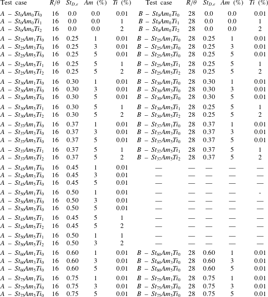
. The governing parameters of all the test cases analysed within the paper are gathered in table 1. The test cases are denoted as ‘
 $A/B$
–
 $St_{a}Am_{b}Ti_{c}$
’, where
 $A/B$
denote thicker/thinner shear layer, respectively,
 $St$
stands for the Strouhal number based on the jet diameter,
 $Am$
denotes the amplitude of external forcing and
 $Ti$
is the turbulence intensity. The subscripts are:
 $a$
,
 $St_{D}\times 100$
;
 $b$
, amplitude of the forcing in
 $\,\%$
;
 $c$
, turbulence intensity in
 $\,\%$
with the lowest
 $Ti=0.01\,\%$
denoted by
 $c=0$
.
The list of the test cases analysed.

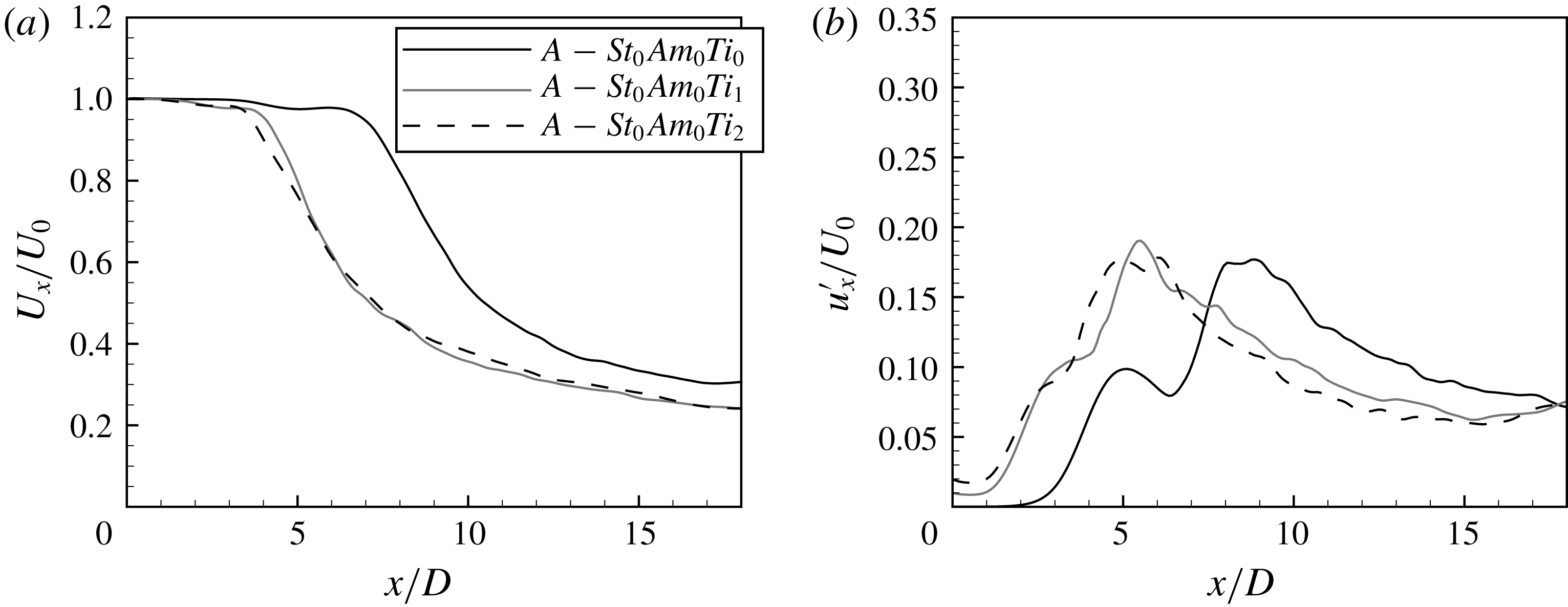
The mean and fluctuating velocity profiles along the jet axis for the first reference cases of the natural jet without external excitation and shear-layer thickness
 $R/\unicode[STIX]{x1D703}=16$
, denoted as
 $A$
–
 $St_{0}Am_{0}Ti_{0}$
,
 $A$
–
 $St_{0}Am_{0}Ti_{1}$
and
 $A$
–
 $St_{0}Am_{0}Ti_{2}$
, are shown in figure 1. The mean and fluctuating velocity profiles are characteristic for the classical Kelvin–Helmholtz instability with the jet potential core length equal to
 $x/D\approx 5$
for the test cases
 $A$
–
 $St_{0}Am_{0}Ti_{1}$
and
 $A$
–
 $St_{0}Am_{0}Ti_{2}$
. For the test case
 $A$
–
 $St_{0}Am_{0}Ti_{0}$
the potential core is much longer. Characteristic for this result is the occurrence of the maximum value of the fluctuating velocity at a distance
 $x/D\approx 5$
. This corresponds to the rolling-up coherent structures. For a higher turbulence level the coherent vortices break up closer to the nozzle exit and their presence is marked by an inflection point on the fluctuating velocity profile at a distance
 $x/D\approx 3$
.
(a) Mean and (b) fluctuating velocity profiles,
 $R/\unicode[STIX]{x1D703}=16$
. Test cases:
 $A$
–
 $St_{0}Am_{0}Ti_{0}$
,
 $A$
–
 $St_{0}Am_{0}Ti_{1}$
and
 $A$
–
 $St_{0}Am_{0}Ti_{2}$
.

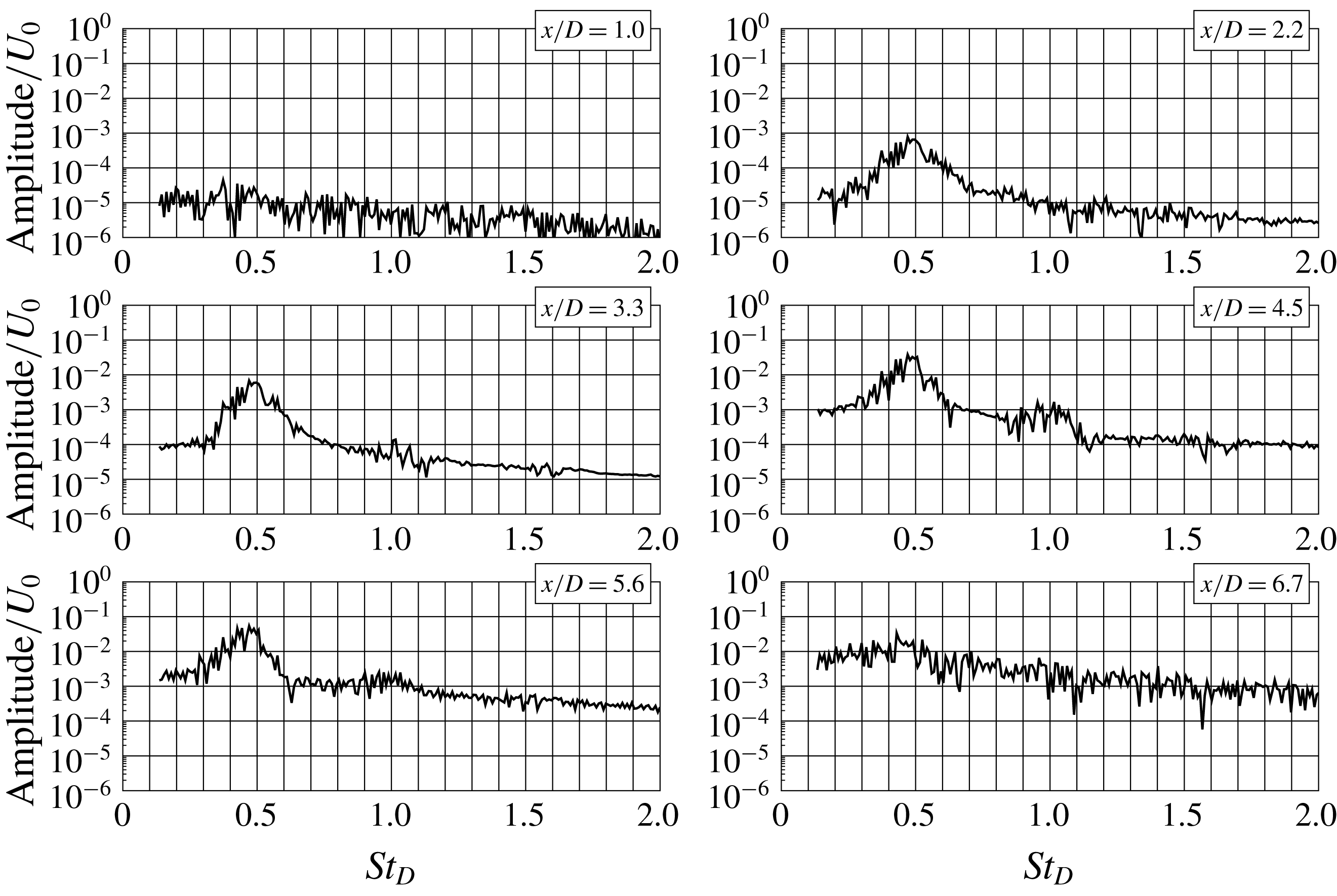
Evolution of spectra of axial velocity fluctuations. Test case:
 $A$
–
 $St_{0}Am_{0}Ti_{0}$
.

Figure 2 shows spectra of the axial velocity component for the test case
 $A$
–
 $St_{0}Am_{0}Ti_{0}$
. It can be seen that the frequency of the fluctuations is characterized by the Strouhal number
 $St_{D}\approx 0.5$
that is in a good agreement with the results of spatial linear stability theory of Michalke (Reference Michalke1984). For the shear layer
 $R/\unicode[STIX]{x1D703}=16$
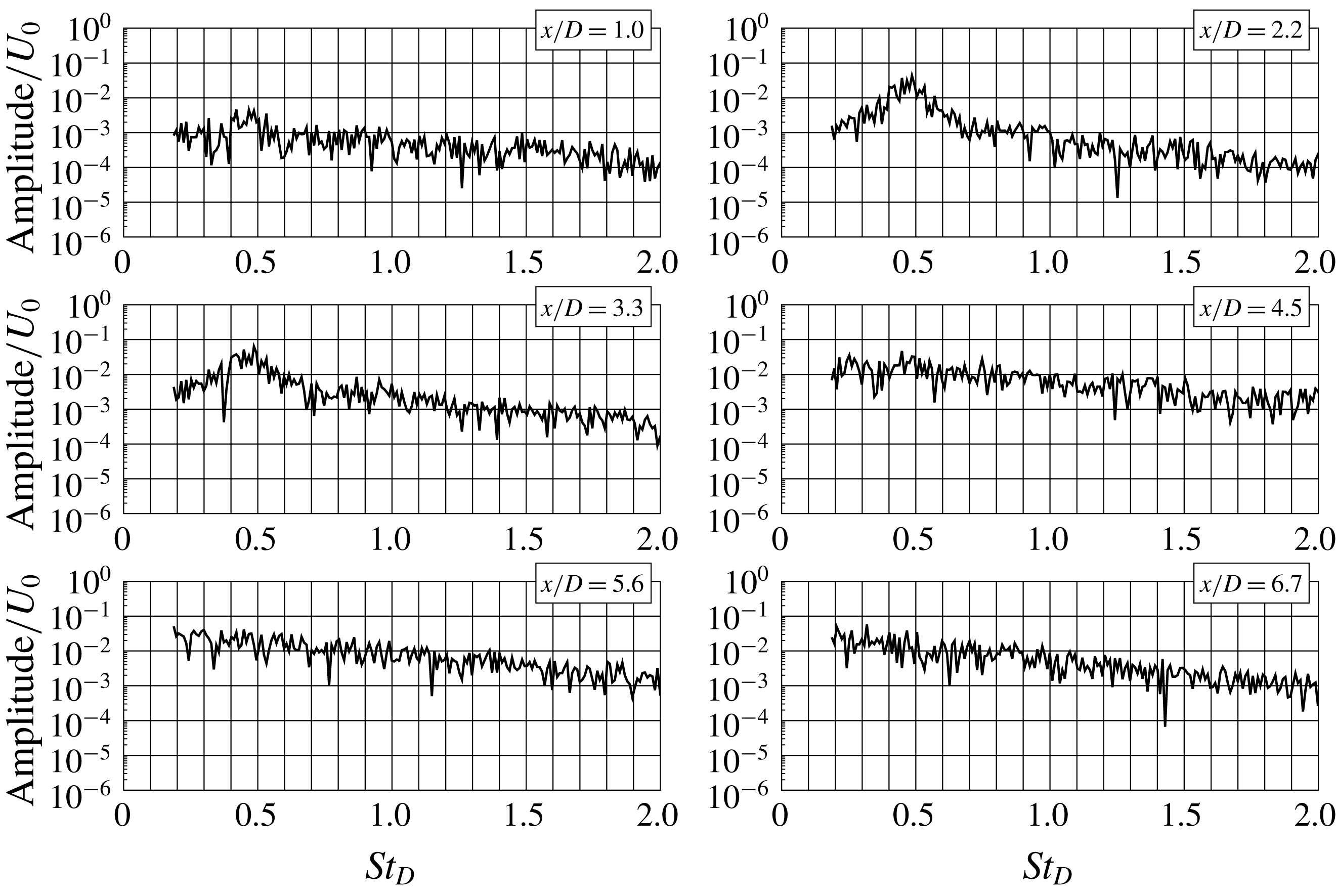
the frequency of the most amplified mode is low, and, as a consequence, the distance between rolling-up vortices is too large for an interaction between them and in effect the vortex pairing process does not occur. Hence, a subharmonic component characteristic for this process does not appear in the spectra. Figure 3 shows the results for turbulence level
 $Ti=1\,\%$
. It can be seen that in the near field for
 $x/D<4$
the spectra are very similar to the previous case
 $A$
–
 $St_{0}Am_{0}Ti_{0}$
. Differences start to be visible further downstream where large-scale structures break up due to an increased turbulence.
Evolution of spectra of axial velocity fluctuations. Test case:
 $A$
–
 $St_{0}Am_{0}Ti_{1}$
.

(a) Mean and (b) fluctuating velocity profiles. Test cases:
 $B$
–
 $St_{0}Am_{0}Ti_{0}$
,
 $B$
–
 $St_{0}Am_{0}Ti_{1}$
and
 $B$
–
 $St_{0}Am_{0}Ti_{2}$
.

The next reference test case (
 $B$
–
 $St_{0}Am_{0}Ti_{0}$
) is characterized by a thinner shear layer with
 $R/\unicode[STIX]{x1D703}=28$
for which the jet remained in the self-sustained regime provided that the turbulence level was sufficiently low (Boguslawski et al.
Reference Boguslawski, Tyliszczak, Drobniak and Asendrych2013; Wawrzak et al.
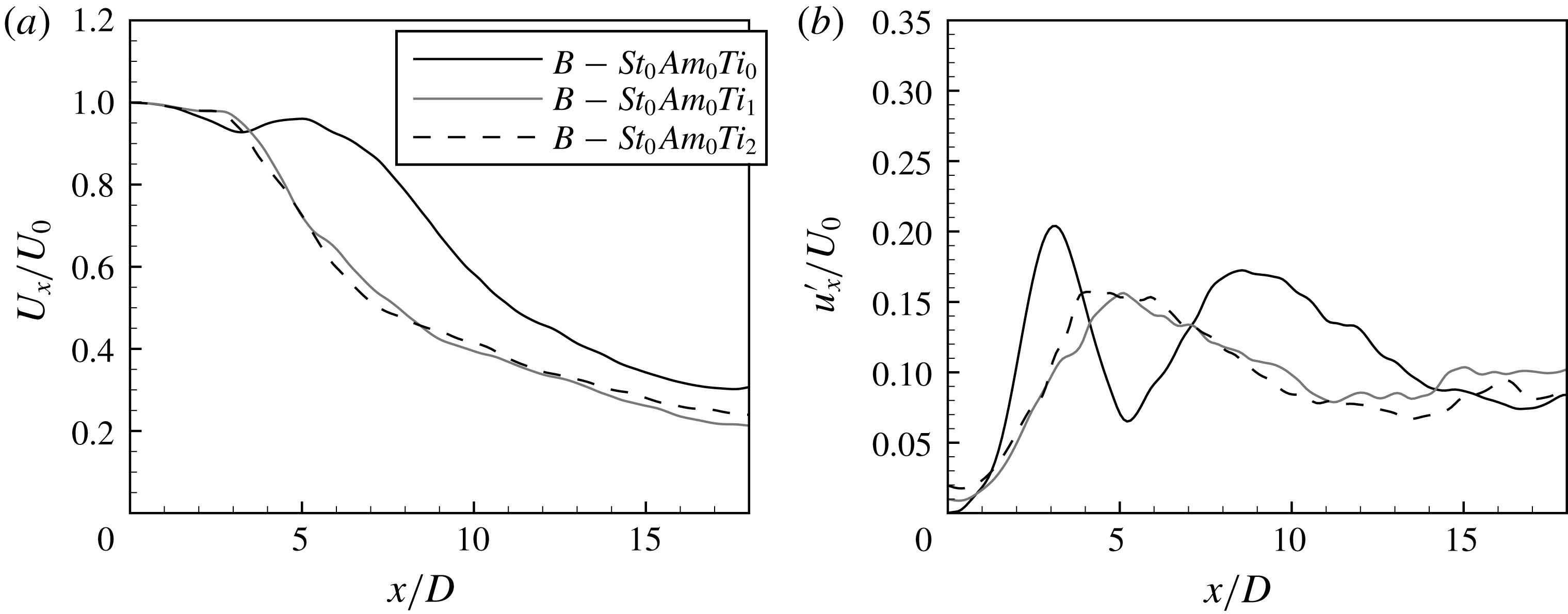
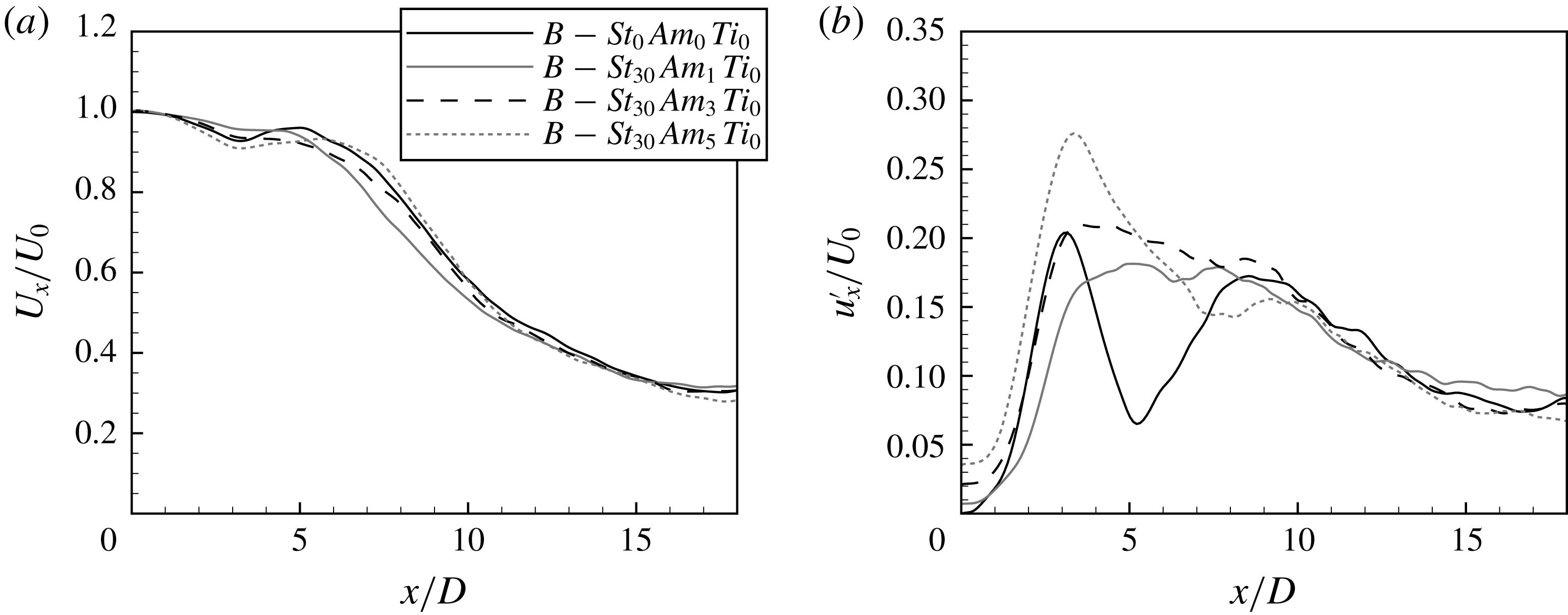
Reference Wawrzak, Boguslawski and Tyliszczak2015). The mean and fluctuating velocity profiles for this test case are shown in figure 4. In the case
 $B$
–
 $St_{0}Am_{0}Ti_{0}$
a large peak on the fluctuating velocity profile equal to
 $0.2U_{0}$
indicates the presence of the self-sustained global jet oscillations. The maximum of the fluctuating velocity profile at a distance
 $x/D\approx 3$
corresponds to a local minimum on the mean velocity profile. By contrast to the previous test case (
 $A$
–
 $St_{0}Am_{0}Ti_{0}$
), under the self-sustained regime, the potential core does not appear. An increase of the inlet turbulence level leads to marked changes in the mean and fluctuating velocity profiles (test cases
 $B$
–
 $St_{0}Am_{0}Ti_{1}$
and
 $B$
–
 $St_{0}Am_{0}Ti_{2}$
). Both are quite similar to the cases with the thicker shear layer
 $R/\unicode[STIX]{x1D703}=16$
(test cases
 $A$
–
 $St_{0}Am_{0}Ti_{1}$
and
 $A$
–
 $St_{0}Am_{0}Ti_{2}$
) presented in figure 1. The potential core is slightly shorter due to higher perturbation growth in the case of thinner shear layer.
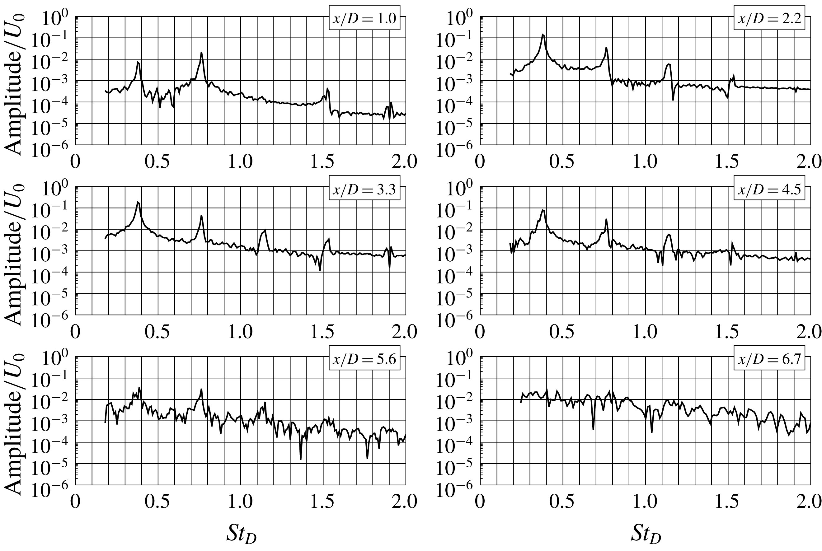
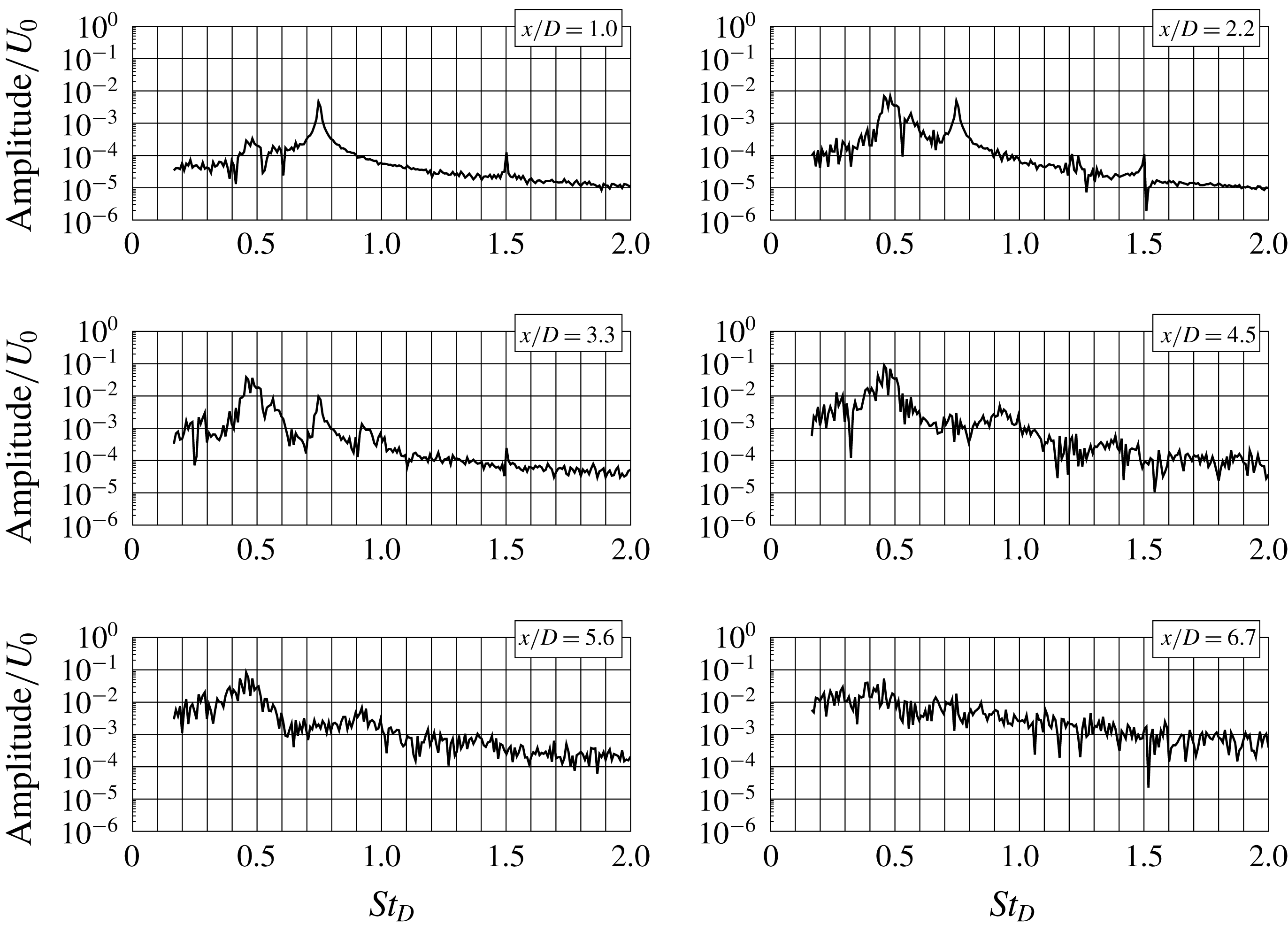
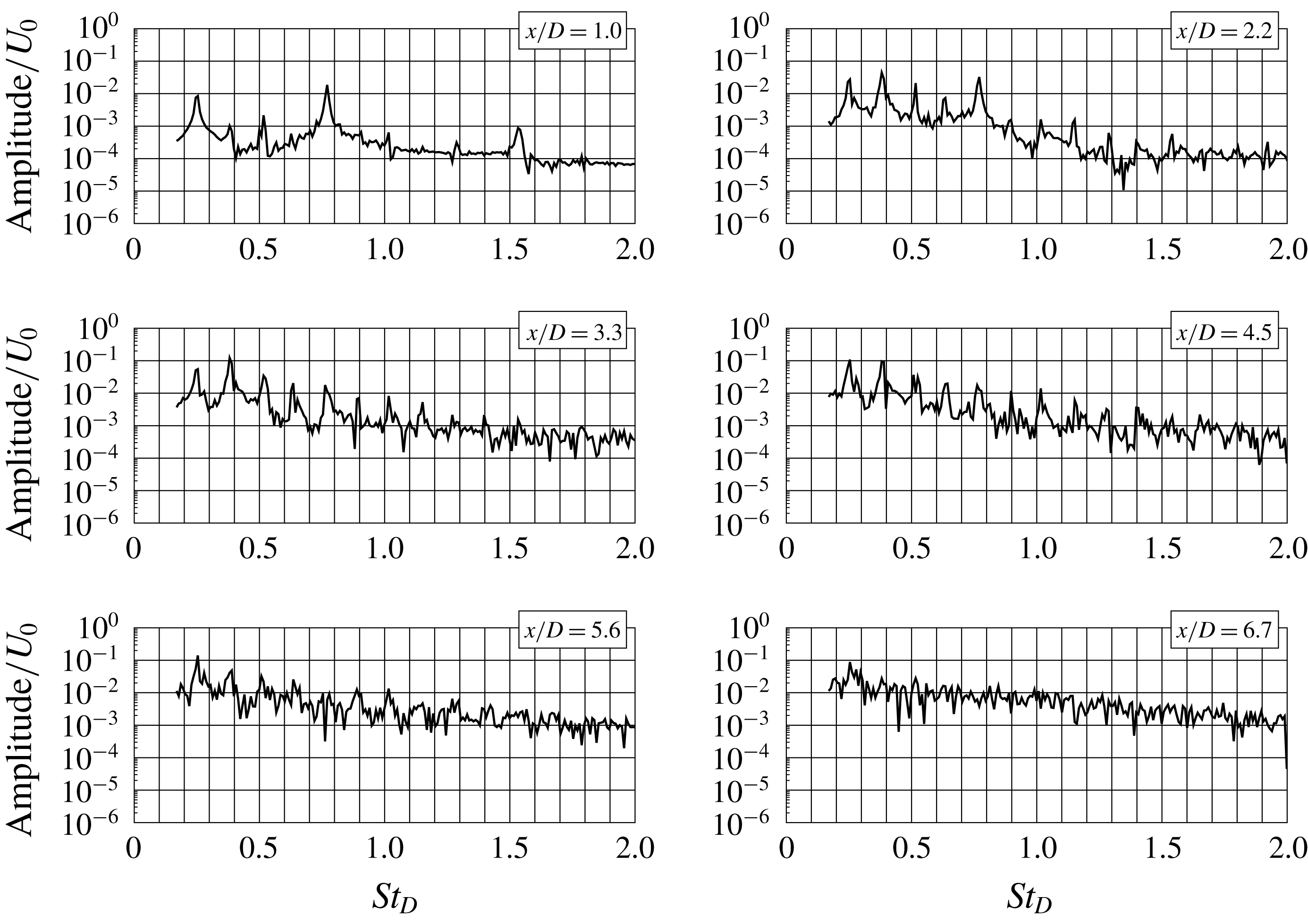
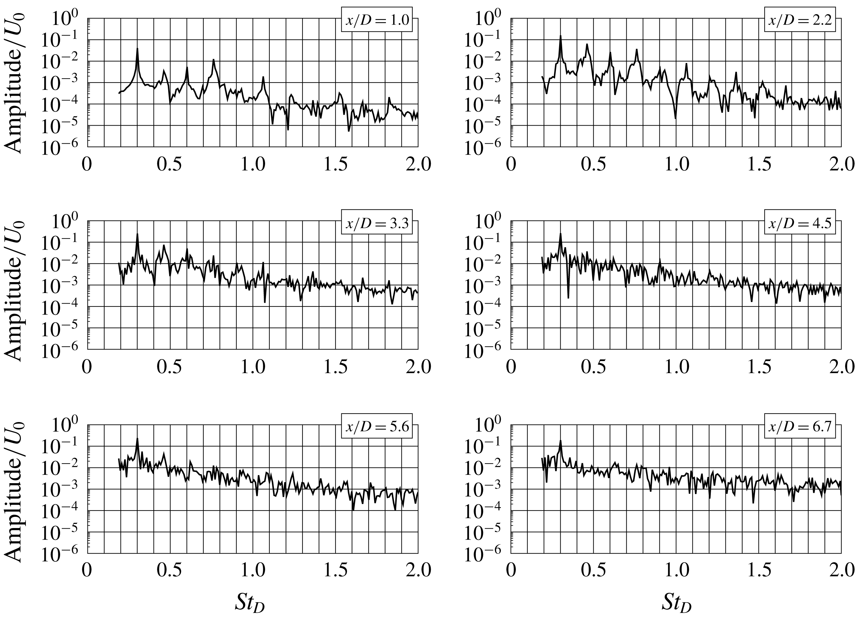
From figure 5, showing the spectra of the axial velocity for the case
 $B$
–
 $St_{0}Am_{0}Ti_{0}$
, one can readily observe that right at the nozzle exit the fundamental mode with non-dimensional frequency
 $St_{D}=0.75$
dominates, while at a short distance
 $x/D\approx 2$
the subharmonic mode is growing indicating the vortex pairing phenomenon. The maximum on the fluctuating velocity profile at a distance
 $x/D\approx 3$
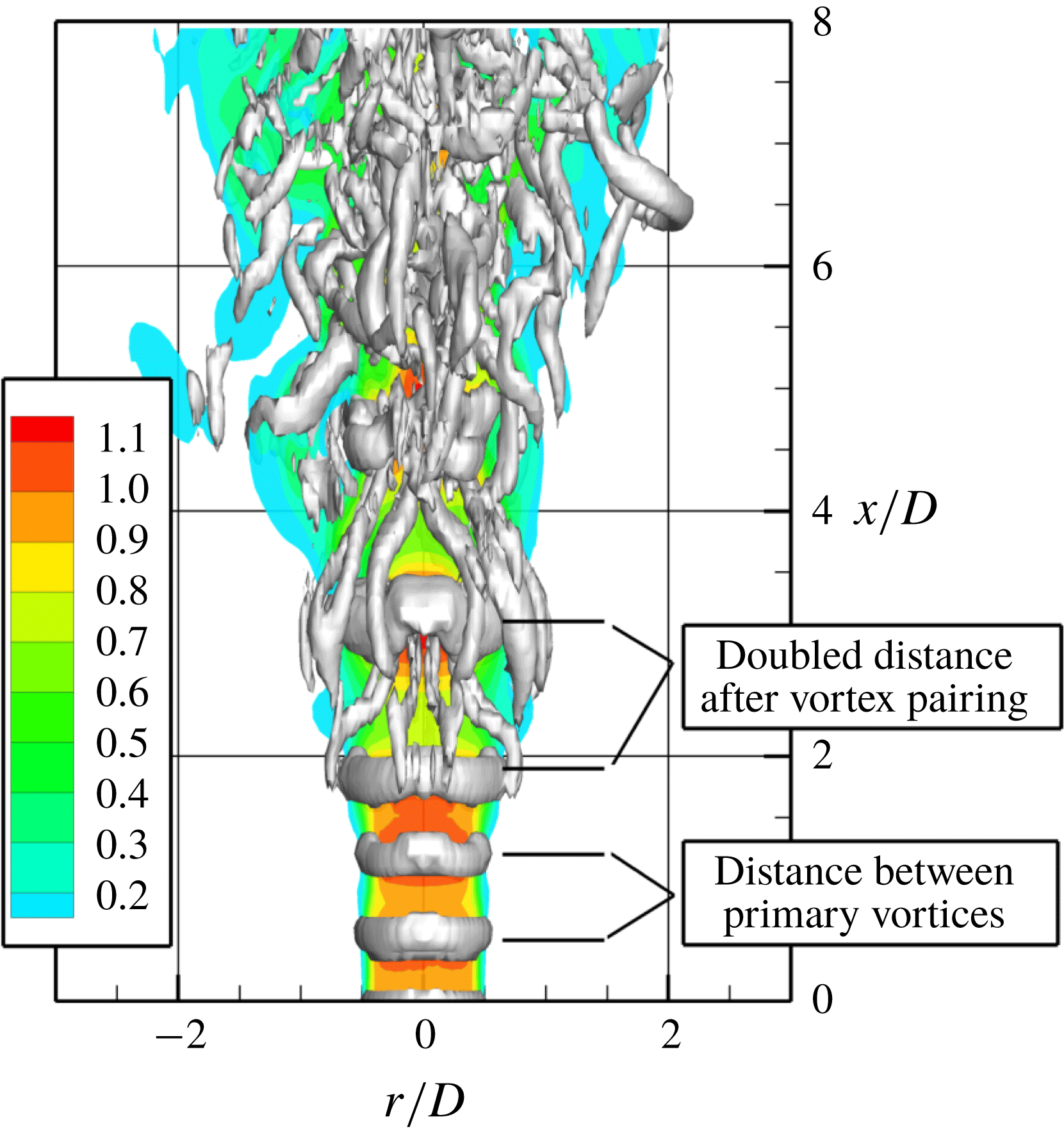
(figure 4) indicates the existence of the developed vortex structures created by the vortex pairing process. This phenomenon is clearly visible in figure 6 showing the
 $Q$
-parameter (
 $Q=1/2(|\boldsymbol{\unicode[STIX]{x1D6FA}}|^{2}-|\mathbf{S}^{2}|)$
, where
 $\boldsymbol{\unicode[STIX]{x1D6FA}}$
is the vorticity tensor and
 $\mathbf{S}$
the strain rate tensor). It is manifested by a larger distance between vortices further downstream (
 $x/D=2$
–
 $4$
) compared to the ones in the near-jet field.
Evolution of spectra of axial velocity fluctuations. Test case:
 $B$
–
 $St_{0}Am_{0}Ti_{0}$
.

 $Q$
-parameter for the jet under the self-sustained regime. Test case:
 $B$
–
 $St_{0}Am_{0}Ti_{0}$
.

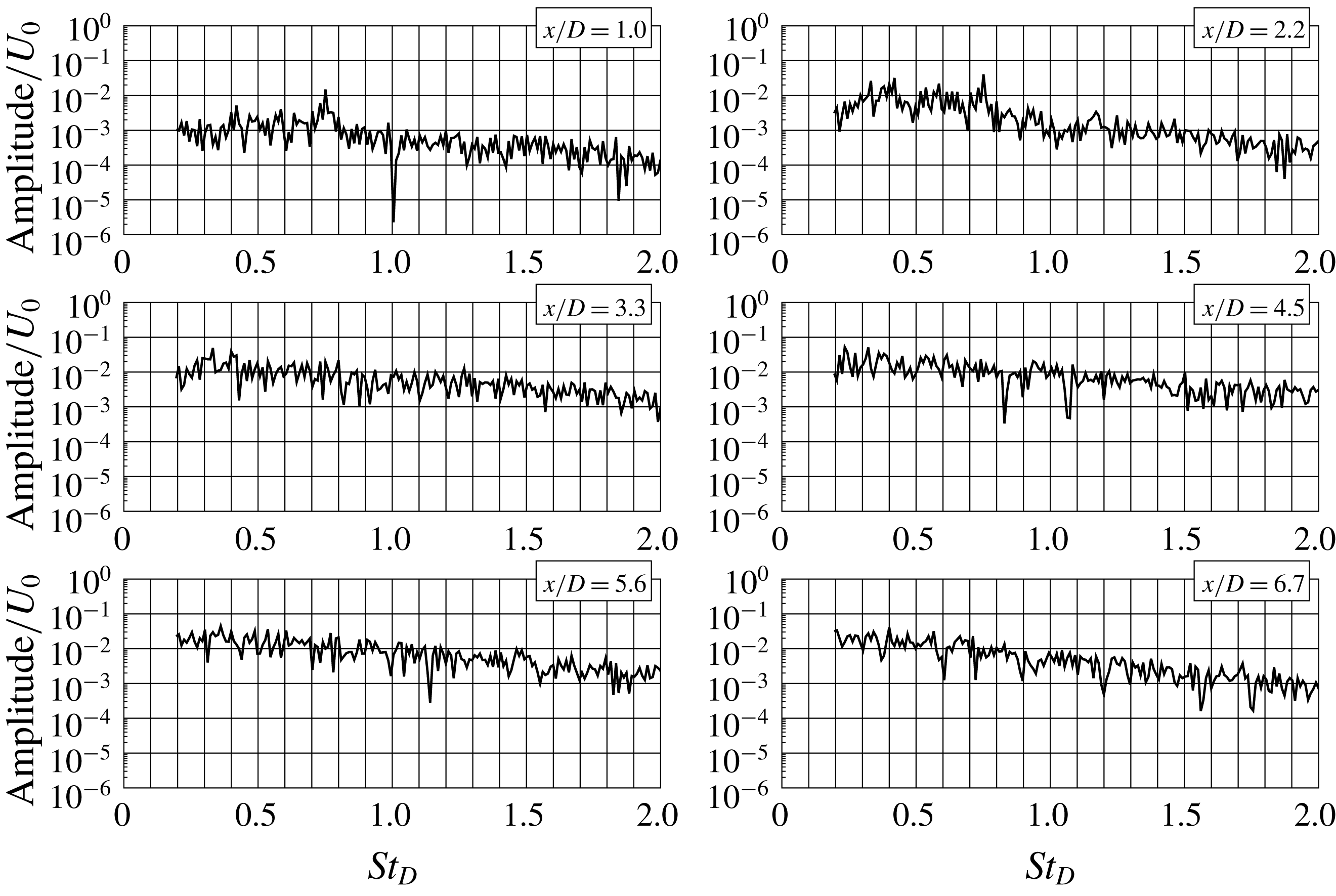
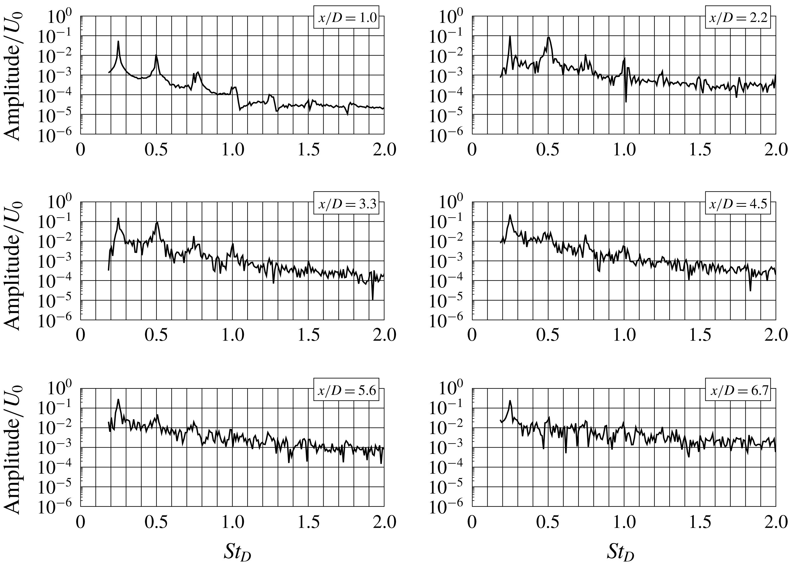
Figure 7 shows the spectra for the case
 $B$
–
 $St_{0}Am_{0}Ti_{1}$
. It can be seen that close to the inlet for
 $x/D<3$
a weak peak characterized with
 $St_{D}\approx 0.75$
is visible. The appearance of peaks with higher frequency for thinner shear layer is characteristic for the Kelvin–Helmholtz instability. Further downstream they disappear as large-scale structures break up. This is exactly what happens with the peak at
 $St_{D}=0.75$
.
Evolution of spectra of axial velocity fluctuations. Test case:
 $B$
–
 $St_{0}Am_{0}Ti_{1}$
.

3.2 Excited jets: test cases with
 $R/\unicode[STIX]{x1D703}=16$

The jet response to an external forcing is first analysed using the cases
 $A$
–
 $St_{25}Am_{1}Ti_{0}$
,
 $A$
–
 $St_{25}Am_{3}Ti_{0}$
and
 $A$
–
 $St_{25}Am_{5}Ti_{0}$
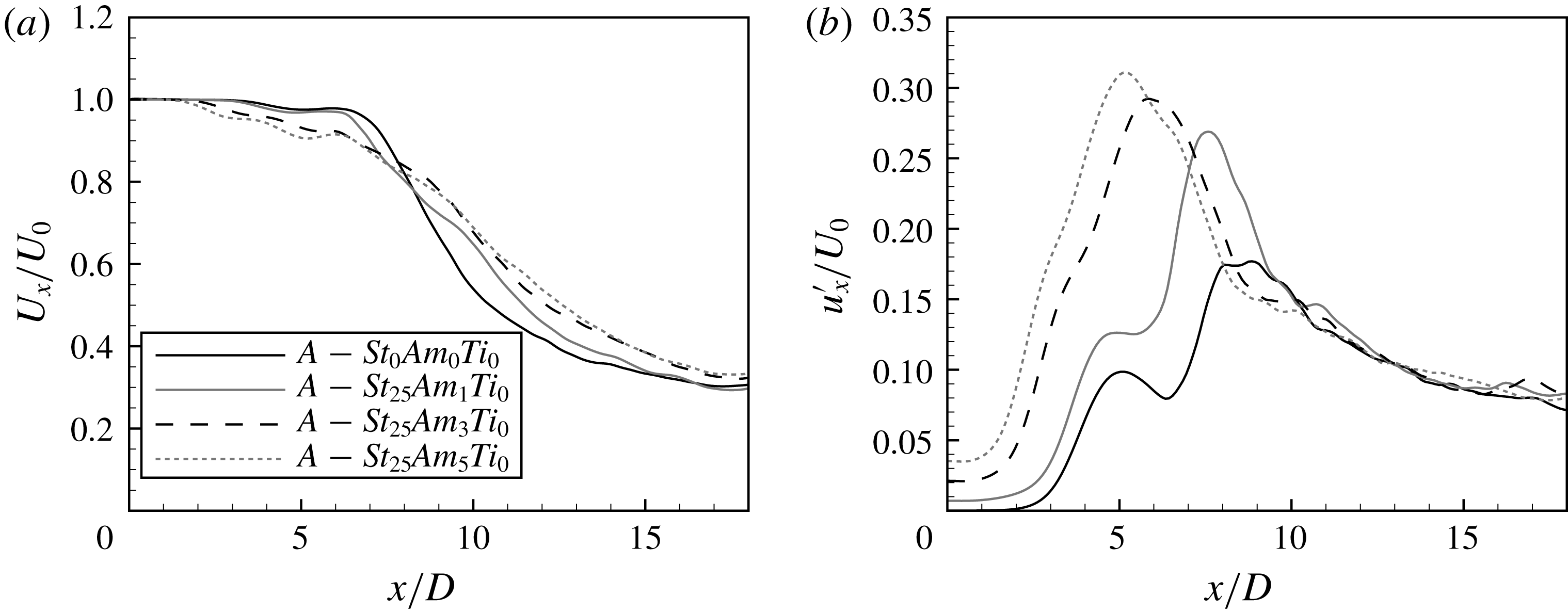
. The influence of the forcing on the mean and fluctuation velocity profiles is shown in figure 8. In the natural jet (test case
 $A$
–
 $St_{0}A_{0}Ti_{0}$
) the fluctuation characterized by the frequency
 $St_{D}=0.25$
does not appear. This is despite that the jet response to the forcing with frequency
 $St_{D,e}=0.25$
is strong and leads to a monotonically growing maximum of the fluctuating velocity at a distance
 $x/D\approx 5$
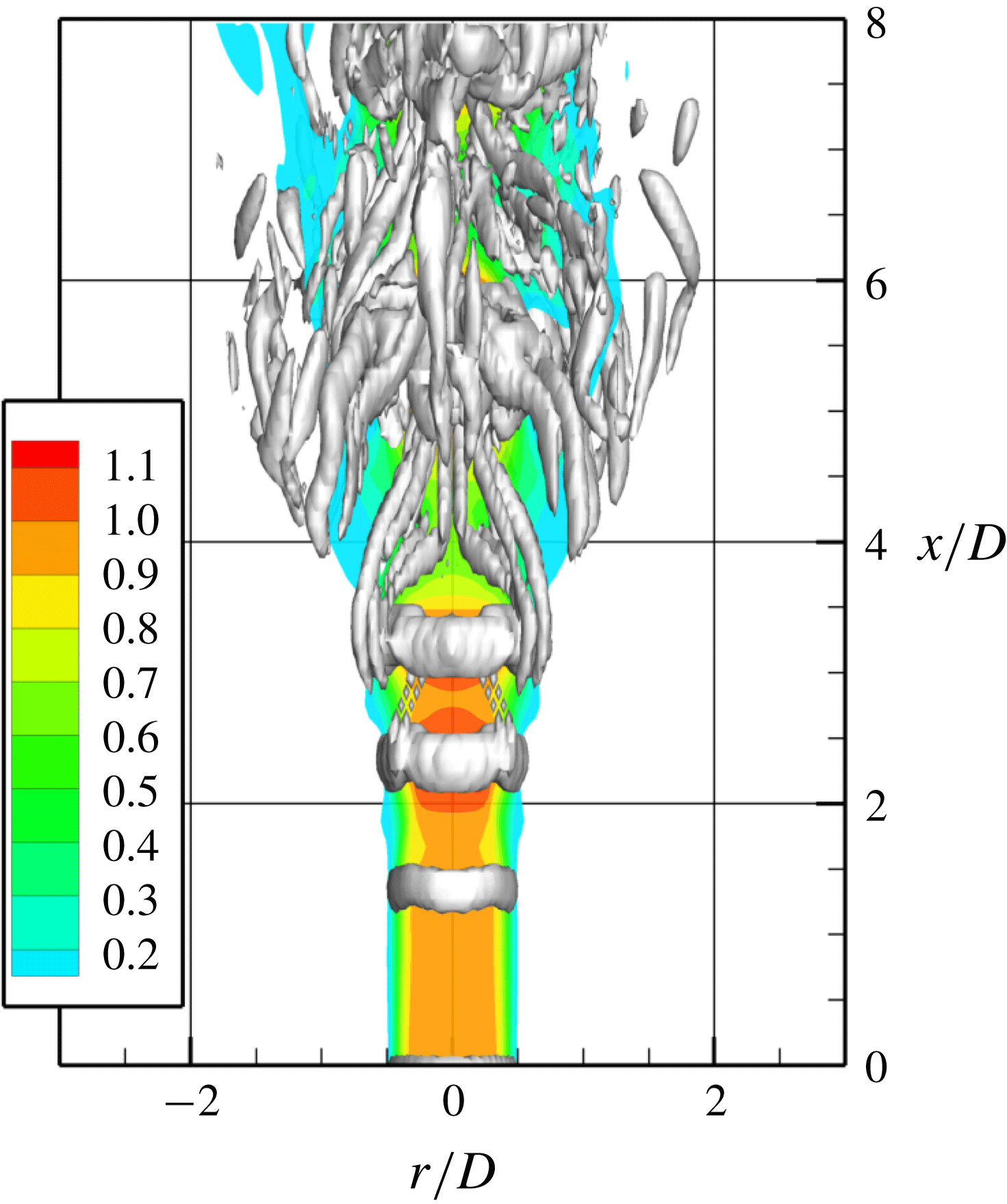
as a function of the forcing amplitude. For the maximum forcing amplitude the peak on the fluctuating velocity profile is approximately three times larger than the peak observed for the natural jet. As can be seen from the spectra shown in figure 9 the mode related to the forcing frequency is well visible in the near-jet field. The jet response to the forcing in this case is an amplification of naturally existing vortex structures rolling-up as a result of the Kelvin–Helmholtz instability. It can be seen from figure 10 showing the
 $Q$
-parameter that at a distance
 $x/D\approx 1$
, well-defined vortical structures are formed.
(a) Mean and (b) fluctuating velocity profiles. Test cases:
 $A$
–
 $St_{0}Am_{1}Ti_{0}$
,
 $A$
–
 $St_{25}Am_{1}Ti_{0}$
,
 $A$
–
 $St_{25}Am_{3}Ti_{0}$
and
 $A$
–
 $St_{25}Am_{5}Ti_{0}$
.

Evolution of spectra of axial velocity fluctuations. Test case:
 $A$
–
 $St_{25}Am_{5}Ti_{0}$
.

 $Q$
-parameter for the forced jet. Test case:
 $A$
–
 $St_{25}Am_{5}Ti_{0}$
.

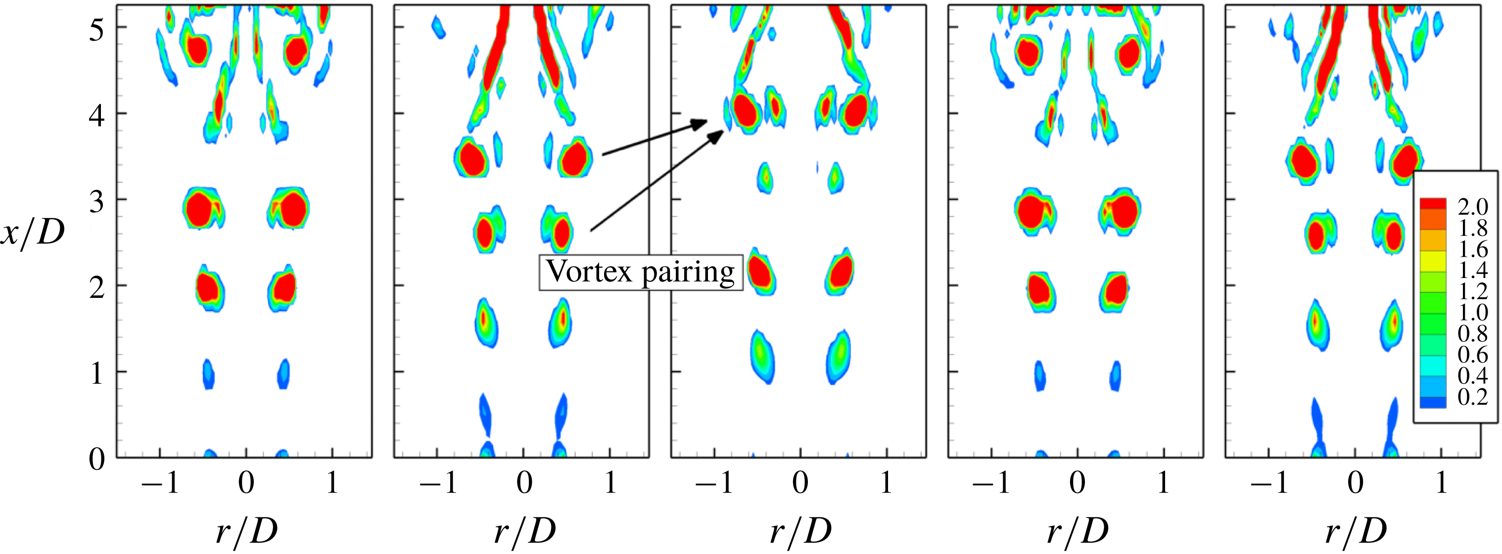
To understand better the vortex dynamics in this case, the contours of the
 $Q$
-parameter are shown in figure 11. It can be seen that at a distance
 $x/D=3$
–
 $4$
from the inlet the vortex pairing process takes place. This observation is confirmed by the analysis of the amplitude evolution of the mode
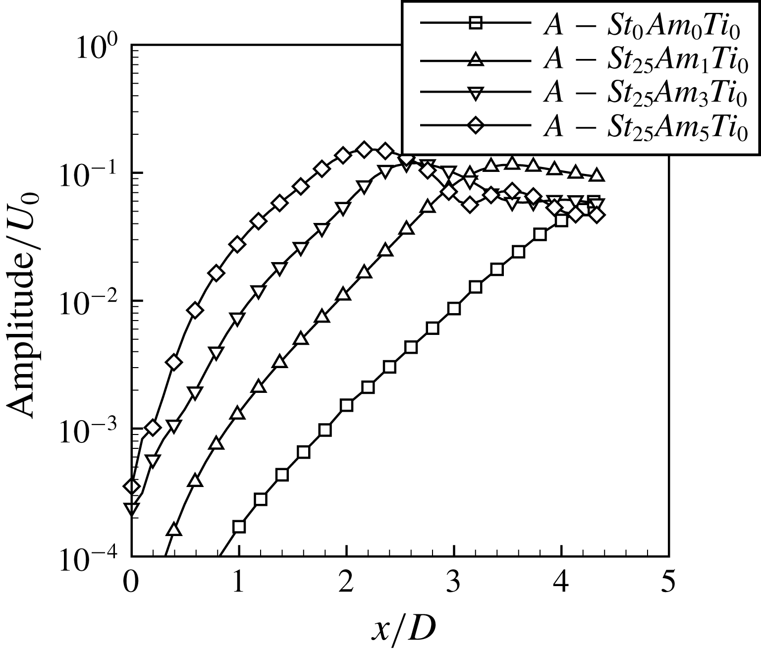
 $St_{D}=0.5$
shown in figure 12. A linear growth of this mode is observed up to a distance
 $x/D=2$
–
 $3$
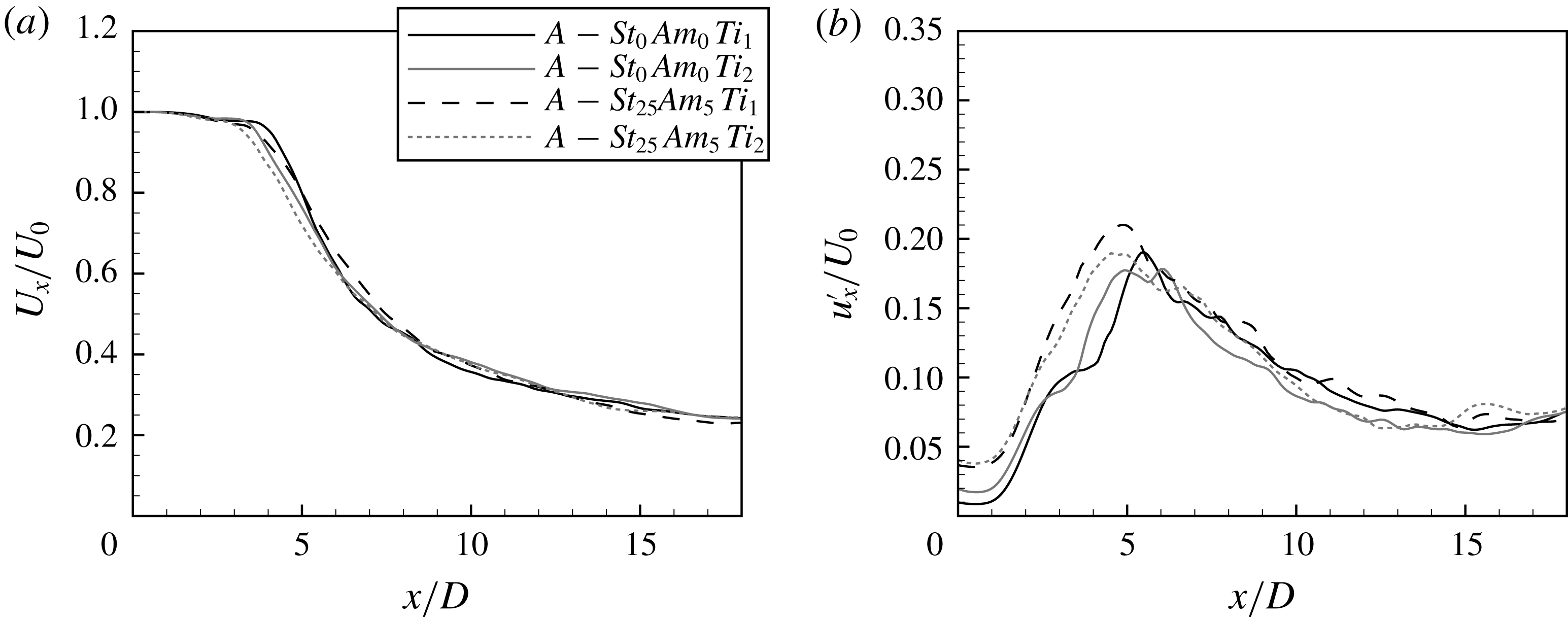
depending on the forcing amplitude. Further downstream the vortex pairing process develops, as visible in figure 11, involving nonlinear interactions. An increased fluctuation intensity due to the forcing in the case of low turbulence level could be interpreted as a result of the vortex pairing not observed in the natural jet. The forcing makes primary structures larger that leads to an interaction between them and pairing. Such a strong amplification of the Kelvin–Helmholtz instability is not observed in the cases with an increased inlet turbulence level,
 $Ti=1\,\%$
and
 $2\,\%$
, for which the results are shown in figure 13. The influence of the forcing on both mean and fluctuating velocity profiles is quite weak. However, a certain increase of the fluctuation level associated with a faster decay of the mean centreline velocity due to forcing is still visible.
Time sequence of the
 $Q$
-parameter iso-contours for the forced jet. Test case:
 $A$
–
 $St_{25}Am_{5}Ti_{0}$
.

Amplitude evolution of the mode
 $St_{D}=0.5$
. Test cases:
 $A$
–
 $St_{25}Am_{0}Ti_{0}$
,
 $A$
–
 $St_{25}Am_{1}Ti_{0}$
,
 $A$
–
 $St_{25}Am_{3}Ti_{0}$
and
 $A$
–
 $St_{25}Am_{5}Ti_{0}$
.

(a) Mean and (b) fluctuating velocity profiles. Test cases:
 $A$
–
 $St_{0}Am_{0}Ti_{1}$
,
 $A$
–
 $St_{0}Am_{0}Ti_{2}$
,
 $A$
–
 $St_{25}Am_{5}Ti_{1}$
and
 $A$
–
 $St_{25}Am_{5}Ti_{2}$
.

Interesting results were obtained for the jet stimulation with a slightly higher non-dimensional frequency
 $St_{D,e}=0.3$
for low turbulence intensity
 $Ti=0.01\,\%$
(
 $A$
–
 $St_{30}Am_{1}Ti_{0}$
,
 $A$
–
 $St_{30}Am_{3}Ti_{0}$
and
 $A$
–
 $St_{30}Am_{5}Ti_{0}$
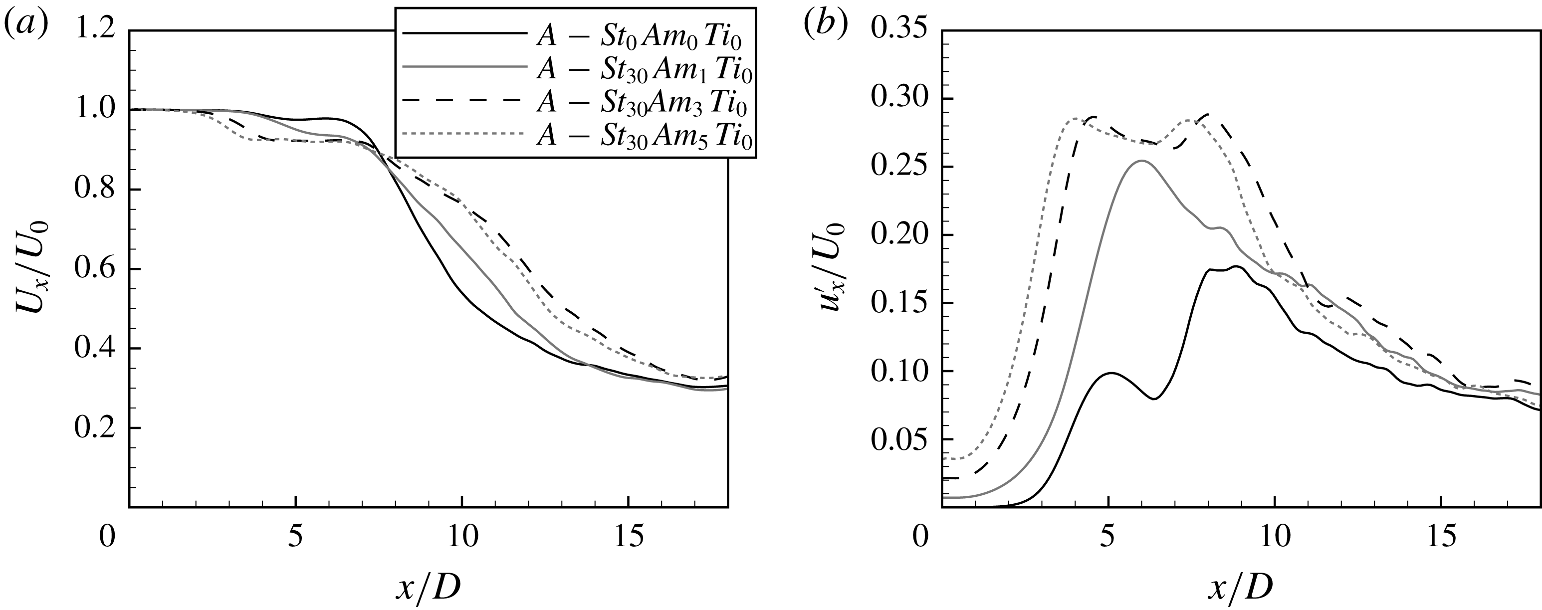
). The mean and fluctuating velocity profiles along the jet axis are shown in figure 14. The forcing with an amplitude 1 % amplifies significantly the fluctuations but does not change the location of the maximum, while the forcing with the higher amplitudes 3 % and 5 % shifts the maximum of the fluctuating velocity upstream without a significant amplification compared to the forcing with
 $1\,\%$
amplitude.
(a) Mean and (b) fluctuating velocity profiles. Test cases:
 $A$
–
 $St_{0}Am_{0}Ti_{0}$
,
 $A$
–
 $St_{30}Am_{1}Ti_{0}$
,
 $A$
–
 $St_{30}Am_{3}Ti_{0}$
and
 $A$
–
 $St_{30}Am_{5}Ti_{0}$
.

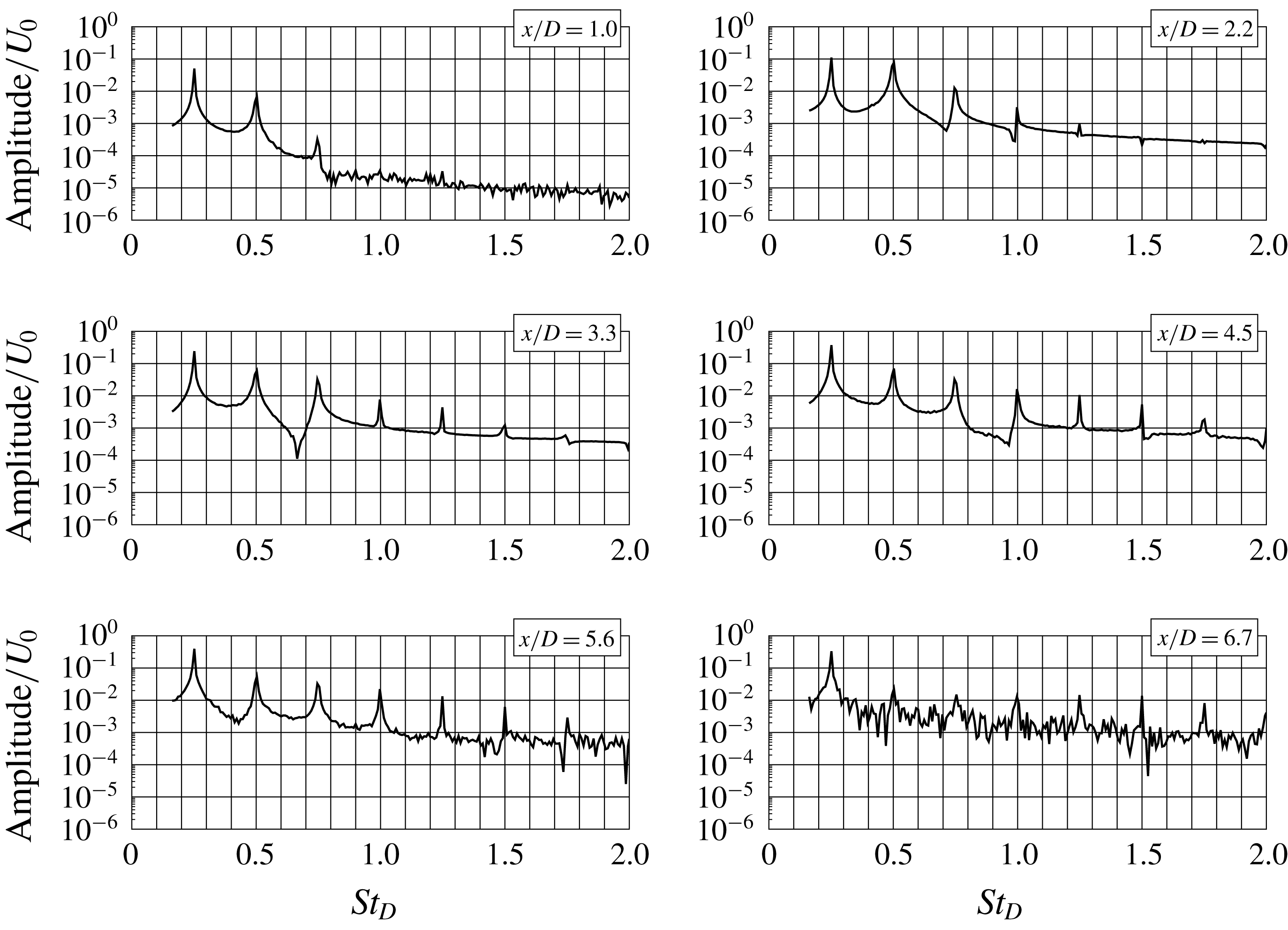
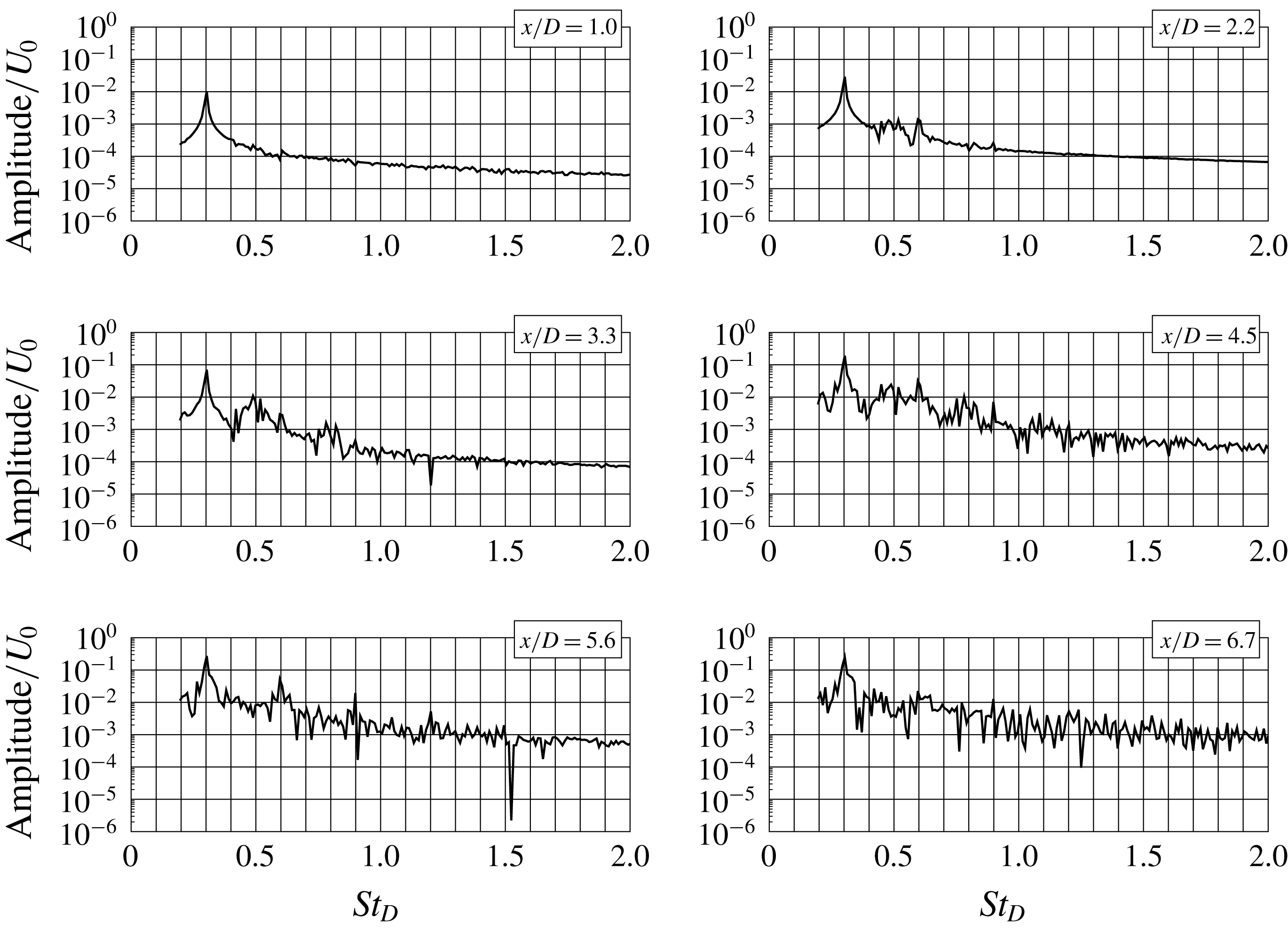
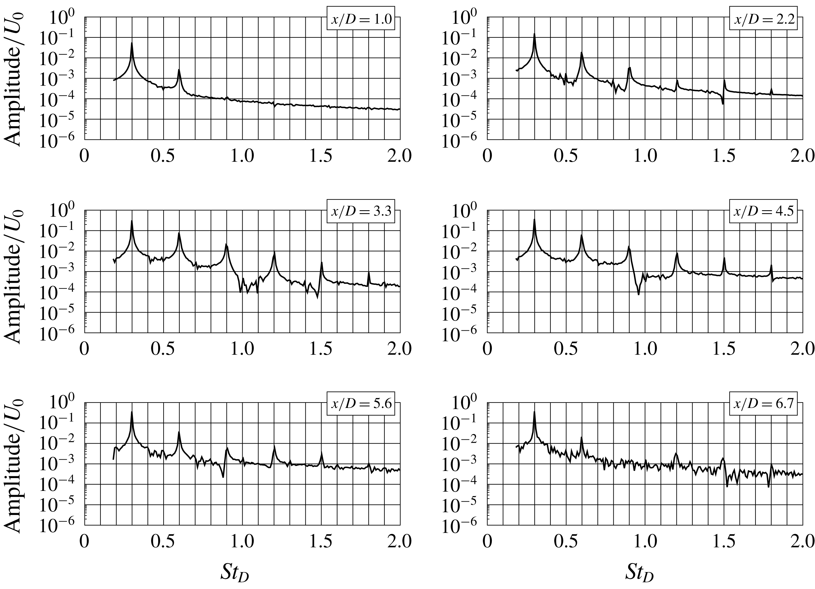
A careful analysis of the evolution of axial velocity spectra shown in figure 15 indicates that for the amplitude
 $Am=1\,\%$
there are two distinct peaks in the spectra at a distance
 $x/D=3.3$
–
 $4.5$
, i.e. one at
 $St_{D}=0.3$
and another weaker one with frequency
 $St_{D}=0.5$
corresponding to the frequency of the mode present in the natural jet. Examination of the spectra in the case of the higher forcing amplitude, shown in figure 16, indicates that the modes corresponding to the forcing frequency and its harmonics dominate in the whole flow field that results in significantly different mean and fluctuating velocity profiles compared to the weakest forcing (see figure 14).
Evolution of spectra of axial velocity fluctuations. Test case:
 $A$
–
 $St_{30}Am_{1}Ti_{0}$
.

Evolution of spectra of axial velocity fluctuations. Test case:
 $A$
–
 $St_{30}Am_{5}Ti_{0}$
.

Amplitude evolution of the mode
 $St_{D}=0.6$
. Test cases:
 $A$
–
 $St_{30}Am_{1}Ti_{0}$
,
 $A$
–
 $St_{30}Am_{3}Ti_{0}$
and
 $A$
–
 $St_{30}Am_{5}Ti_{0}$
.

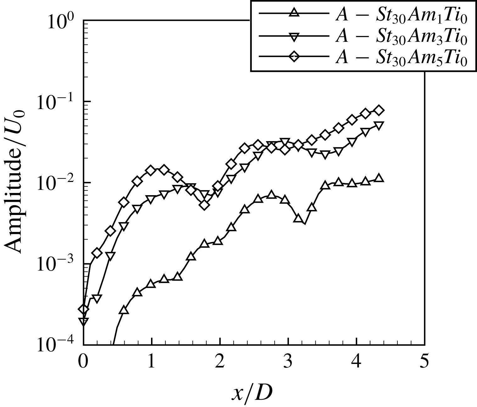
Differences in the jet response to the forcing with amplitude
 $1\,\%$
and with higher amplitudes can be explained through an analysis of the amplitude evolution of the mode
 $St_{D}=0.6$
shown in figure 17. For the weakest forcing a nearly linear growth of the perturbation is observed up to
 $x/D=2.5$
, which means that the vortex pairing process is completed at the same distance as for the forcing with
 $St_{D,e}=0.25$
(see figure 12). Hence the jet response to the weakest forcing with frequency
 $St_{D,e}=0.3$
is qualitatively similar to the jet response with the forcing
 $St_{D,e}=0.25$
. A change is observed for stronger forcing that is reflected in a different development of the perturbation, namely the nonlinear interactions are visible much closer to the inlet (
 $x/D=1$
). This means that in the case of the forcing with frequency
 $St_{D,e}=0.3$
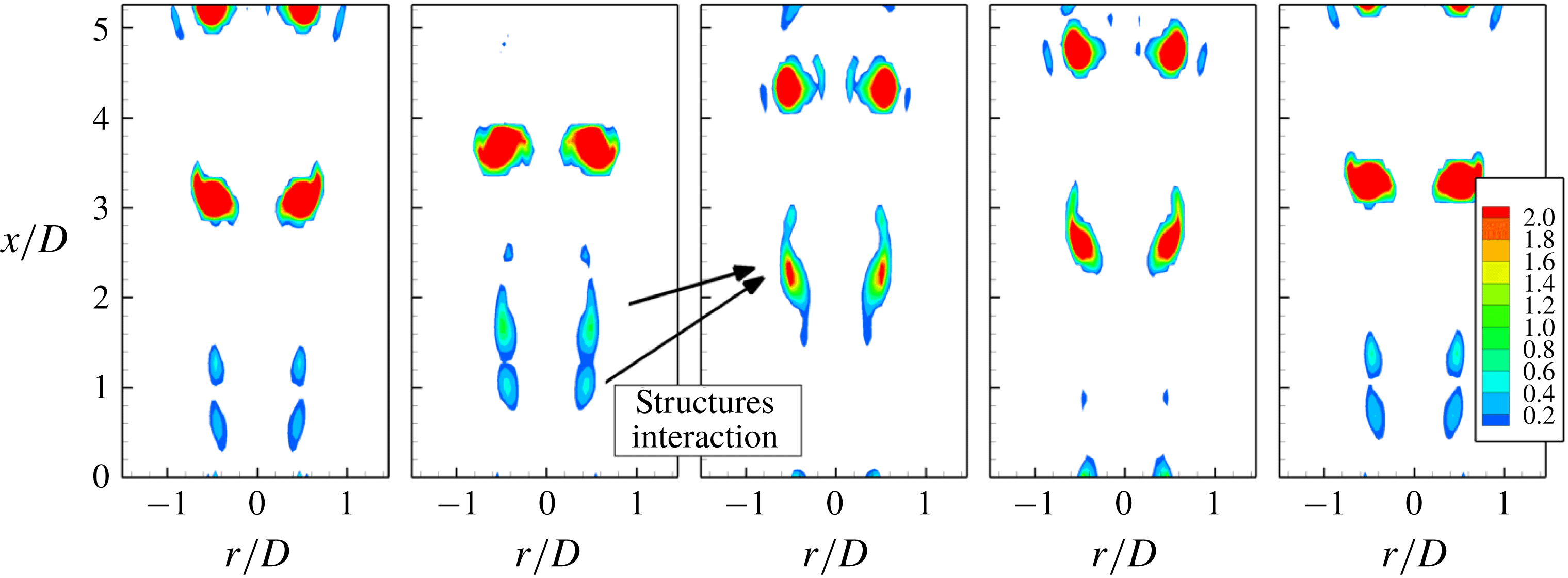
the primary structures released by the Kelvin–Helmholtz instability are located close enough to each other that nonlinear interactions limit their further growth. This observation can be confirmed by an analysis of the
 $Q$
-parameter iso-contours shown in figure 18. It can be seen that at a distance
 $x/D=1$
the perturbations released by the Kelvin–Helmholtz instability interact and form larger structures at a distance
 $x/D=3$
–
 $4$
. At this location the maximum of the fluctuating velocity is observed as shown in figure 14.
Time sequence of the
 $Q$
-parameter iso-contours for the forced jet. Test case:
 $A$
–
 $St_{30}Am_{5}Ti_{0}$
.

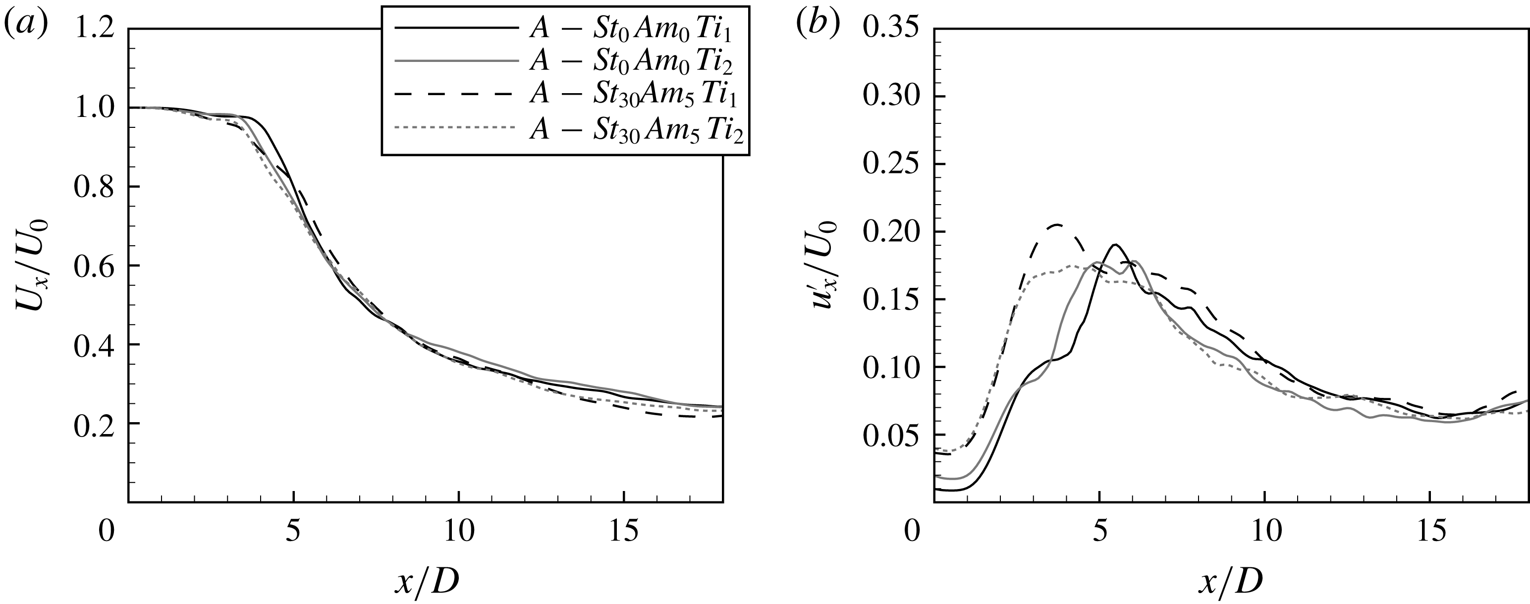
In the case of the increased inlet turbulence intensity (
 $Ti=1\,\%$
and
 $2\,\%$
) the influence of the forcing with frequency
 $St_{D,e}=0.3$
and amplitude
 $Am=5\,\%$
on the mean and fluctuating velocity profiles is much weaker than in the case of
 $Ti=0.01\,\%$
as shown in figure 19. The maximum of the fluctuating velocity profile is located at a distance
 $x/D=3$
–
 $4$
as in the case of low inlet turbulence level (see figure 14). The mean velocity profile is practically unaffected by the forcing. However, it should be stressed that the influence of forcing on the fluctuations in the near-jet field
 $x/D=2$
–
 $3$
is significantly stronger compared to the forcing with
 $St_{D,e}=0.25$
and
 $Ti=1\,\%$
and
 $2\,\%$
(see figure 13). The comparison of the jet response to the forcing with slightly different frequencies
 $St_{D,e}=0.25$
and
 $0.3$
reveals different scenarios of instability development. For frequency
 $St_{D,e}=0.25$
, that is the subharmonic of the natural Kelvin–Helmholtz instability, the perturbation grows linearly up to a distance
 $x/D=2$
–
 $3$
and then the vortex pairing generates larger structures (see figure 12). In the case of an increased turbulence level the jet does not respond to the external forcing. The primary vortices are distorted by turbulence before the pairing process occurs. On the contrary, in the case of higher frequency the nonlinear interactions take place much closer to the inlet producing larger structures. It seems that in the case of an increased turbulence level the primary structures undergo the pairing process before they are distorted by turbulence. Larger and stronger vortices are more resistant to turbulence. In this case the external forcing amplifies the jet instability even when the turbulence level is higher.
(a) Mean and (b) fluctuating velocity profiles. Test cases:
 $A$
–
 $St_{0}Am_{0}Ti_{1}$
,
 $A$
–
 $St_{0}Am_{0}Ti_{2}$
,
 $A$
–
 $St_{30}Am_{5}Ti_{1}$
and
 $A$
–
 $St_{30}Am_{5}Ti_{2}$
.

The mean and fluctuating velocity profiles for Strouhal number
 $St_{D,e}=0.37$
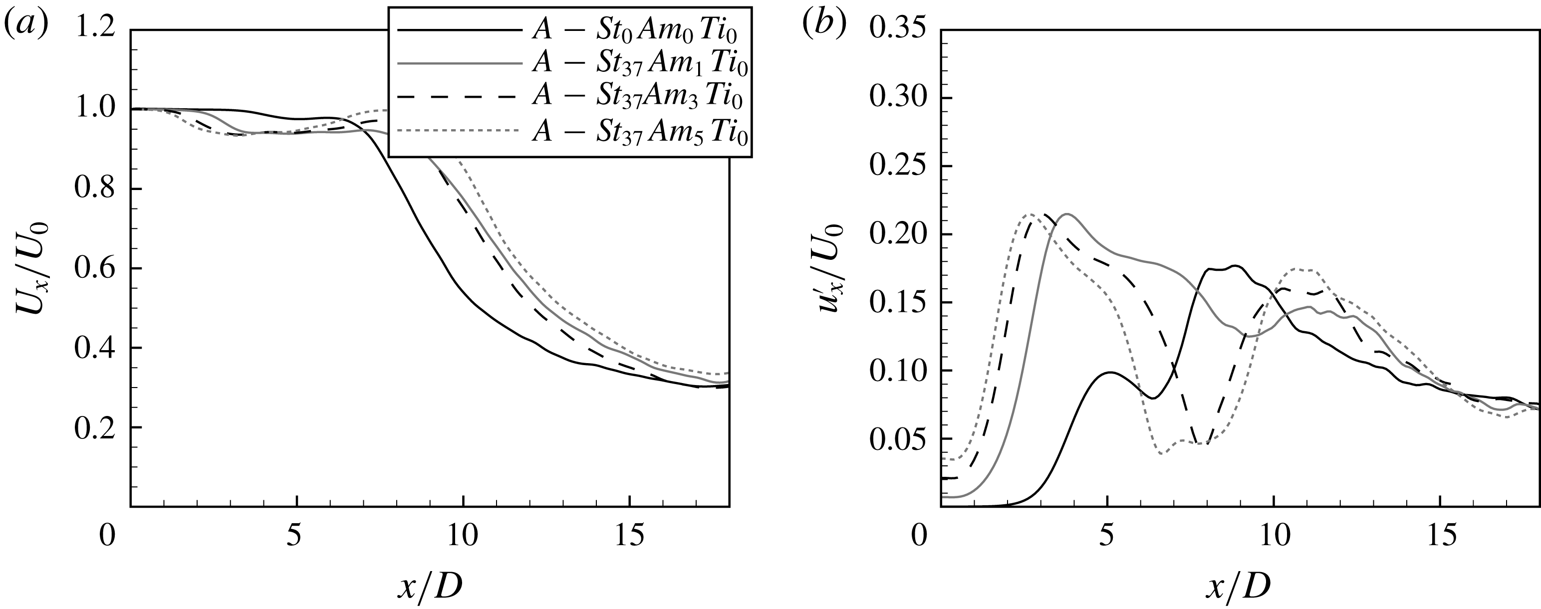
, which means the frequency corresponding to the subharmonic of the self-sustained mode obtained for the jet with sufficiently thin shear layer and without external stimulation, are shown in figure 20. It can be seen that for this particular frequency even the lowest amplitude of the forcing leads to a significant change in the jet instability regime. A further increase in the forcing amplitude has no effect on the maximum of the fluctuating velocity and causes only a certain shift of its location in the direction of the inlet.
(a) Mean and (b) fluctuating velocity profiles. Test cases:
 $A$
–
 $St_{0}Am_{0}Ti_{0}$
,
 $A$
–
 $St_{37}Am_{1}Ti_{0}$
,
 $A$
–
 $St_{37}Am_{3}Ti_{0}$
and
 $A$
–
 $St_{37}Am_{5}Ti_{0}$
.

Evolution of spectra of axial velocity fluctuations. Test case:
 $A$
–
 $St_{37}Am_{5}Ti_{0}$
.

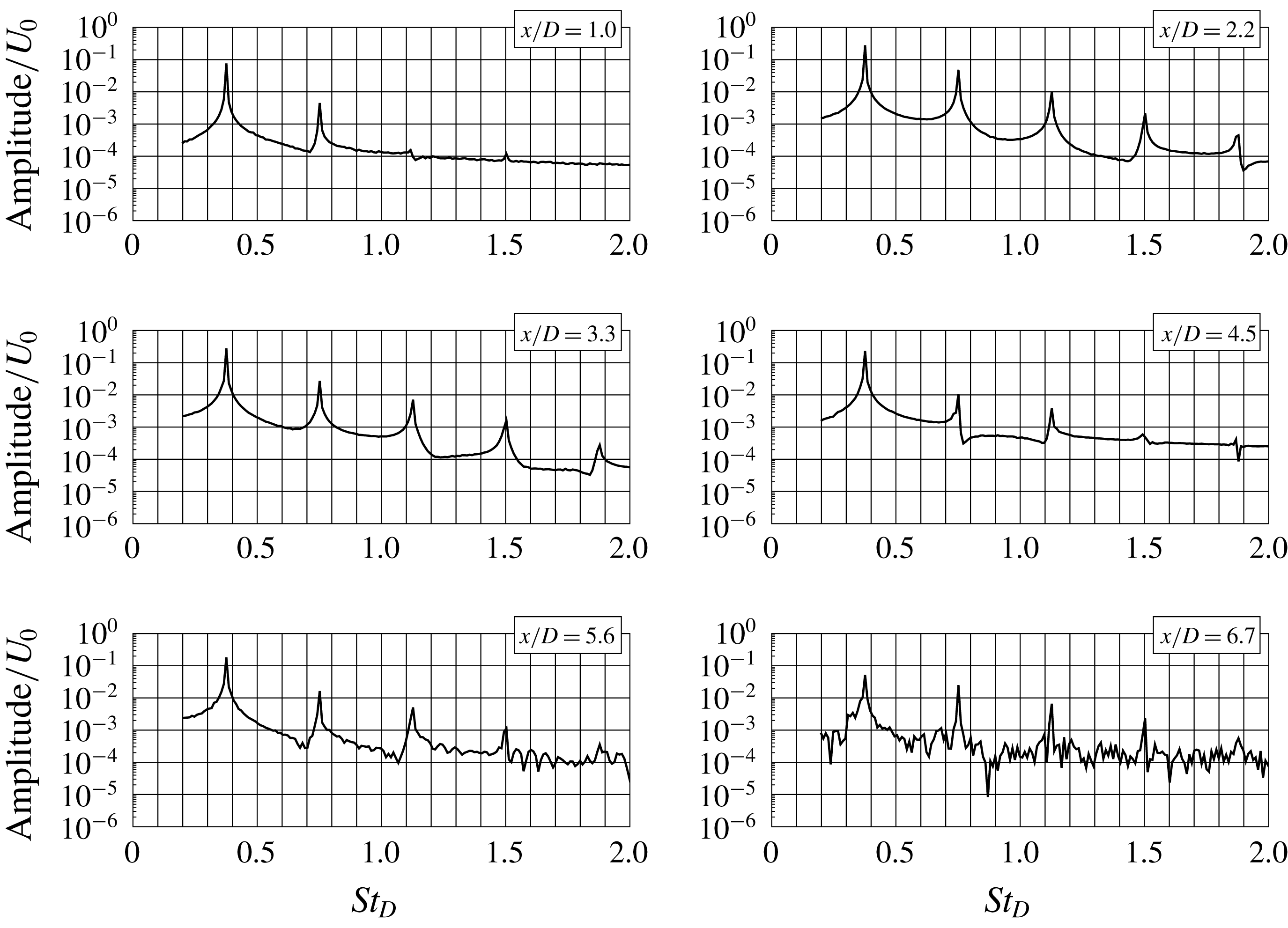
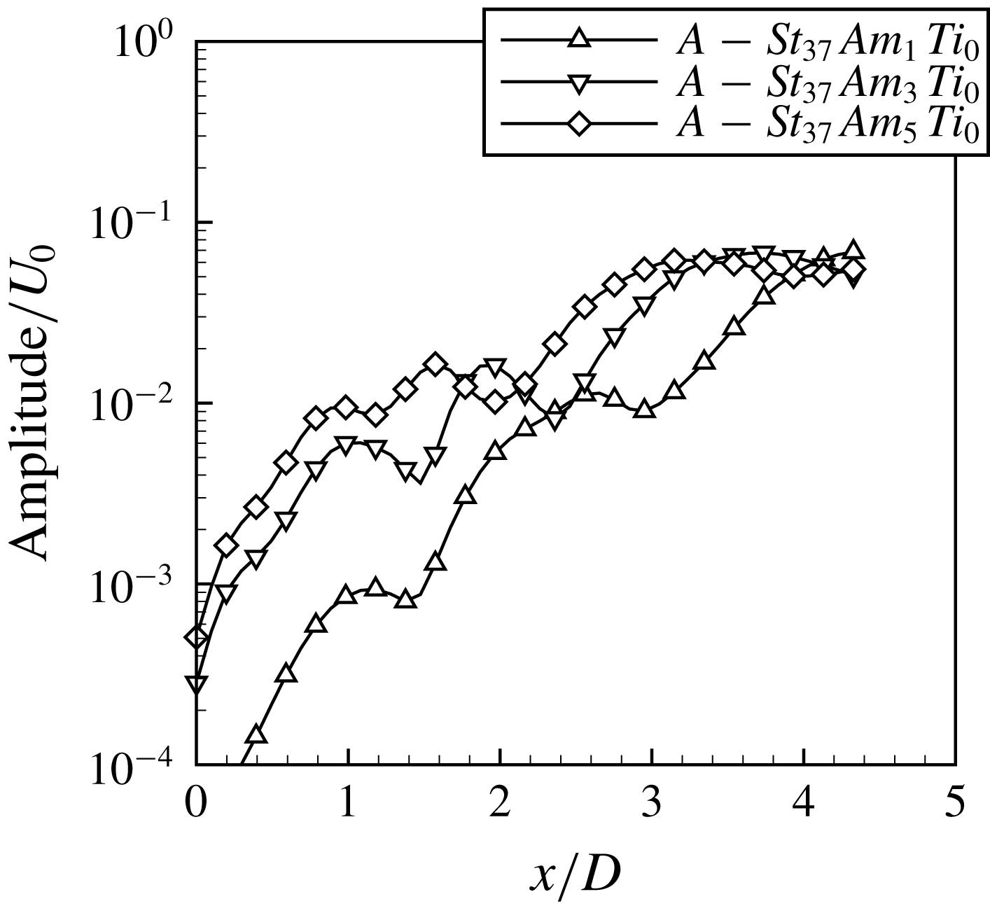
The analysis of the spectra shown in figure 21 for amplitude 5 % shows that the peaks corresponding to the stimulation frequency and its harmonics are present along the whole jet. Figure 22 shows the evolution of the amplitude of the mode
 $St_{D}=0.75$
. It can be seen that for all the forcing amplitudes the profiles are qualitatively similar. A linear growth is observed only for
 $x/D<1$
. Further downstream the nonlinear interactions form larger structures leading to the maximum of the flow oscillations at a distance
 $x/D=2$
–
 $3$
(see figure 20). It should be stressed here that forcing the jet with
 $St_{D,e}=0.37$
corresponding to the subharmonic of the self-sustained mode in the case of shear layer
 $R/\unicode[STIX]{x1D703}=16$
does not introduce the self-sustained regime. As shown by Boguslawski et al. (Reference Boguslawski, Tyliszczak, Drobniak and Asendrych2013) in the case of the self-sustained regime a high level of oscillations is observed right at the inlet and the perturbation growth is independent of the forcing amplitude. In figure 22 a linear growth is observed up to
 $x/D=1$
and the perturbation level is sensitive to the forcing amplitude.
Amplitude evolution of the mode
 $St_{D}=0.75$
. Test cases:
 $A$
–
 $St_{37}Am_{1}Ti_{0}$
,
 $A$
–
 $St_{37}Am_{3}Ti_{0}$
and
 $A$
–
 $St_{37}Am_{5}Ti_{0}$
.

Comparison of the fluctuating velocity profiles predicted numerically with the experimental data. Test cases: (a)
 $B$
–
 $St_{0}Am_{0}Ti_{0}$
and
 $A$
–
 $St_{37}Am_{5}Ti_{0}$
; (b)
 $A$
–
 $St_{37}Am_{5}Ti_{1}$
and
 $A$
–
 $St_{37}Am_{5}Ti_{2}$
.

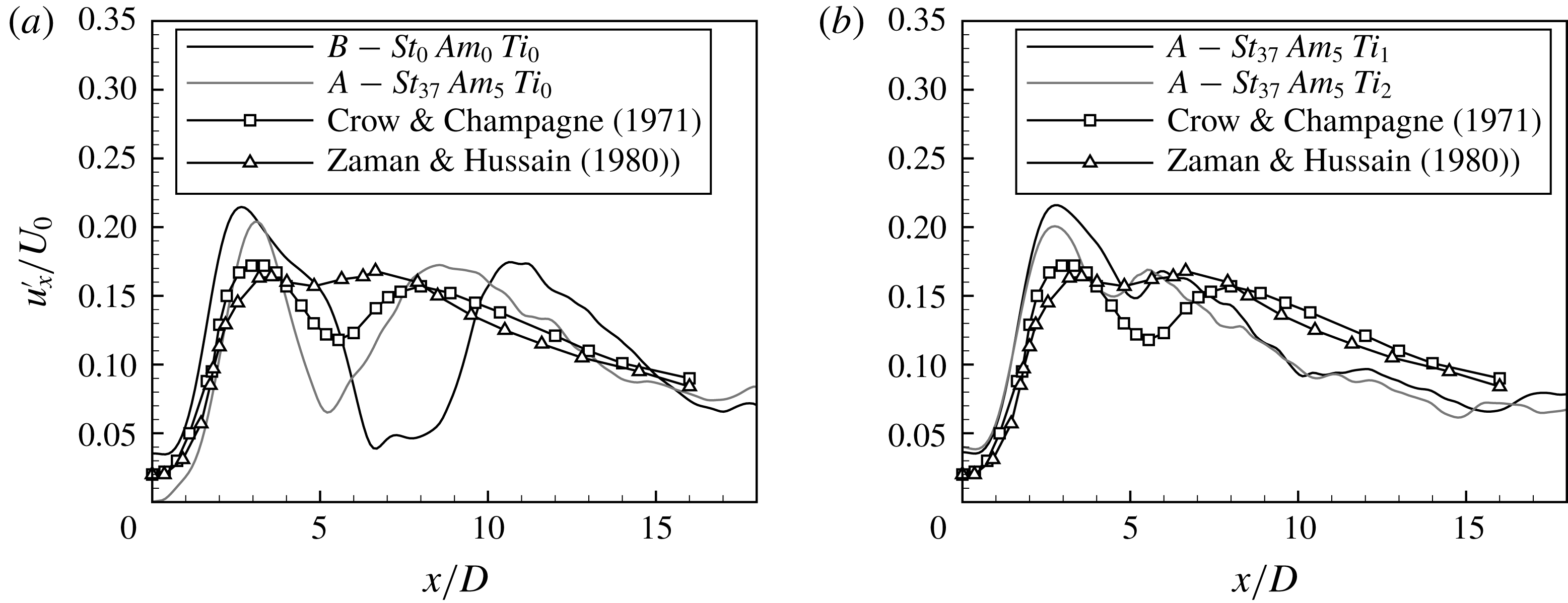
In order to stress the similarity of the preferred mode studied experimentally by Crow & Champagne (Reference Crow and Champagne1971) and by Hussain & Zaman (Reference Hussain and Zaman1980), Zaman & Hussain (Reference Zaman and Hussain1980) and Hussain & Zaman (Reference Hussain and Zaman1981) and the current simulation results, including forced jet and the self-sustained mode, all the results are compared in figure 23(a). Despite that the experimental data were obtained with different Reynolds numbers, especially in the case of the Crow & Champagne (Reference Crow and Champagne1971) experiment, the agreement is very good in terms of the maximum value on the fluctuating velocity profile and its location. Figure 23(b) shows the comparison of fluctuating velocity profiles for two test cases with forcing amplitude
 $5\,\%$
and higher inlet turbulence level. Agreement with the experimental results is even better than for the low inlet turbulence intensity, especially further downstream from the inlet, i.e. for
 $x/D>4$
.
Comparison of the fluctuating velocity profiles predicted numerically with the experimental data. Test cases: (a)
 $A$
–
 $St_{0}Am_{0}Ti_{0}$
,
 $A$
–
 $St_{45}Am_{1}Ti_{0}$
,
 $A$
–
 $St_{45}Am_{3}Ti_{0}$
and
 $A$
–
 $St_{45}Am_{3}Ti_{0}$
; (b)
 $A$
–
 $St_{0}Am_{0}Ti_{0}$
,
 $A$
–
 $St_{50}Am_{1}Ti_{0}$
,
 $A$
–
 $St_{50}Am_{3}Ti_{0}$
and
 $A$
–
 $St_{50}Am_{3}Ti_{0}$
.

Comparison of the fluctuating velocity profiles predicted numerically with the experimental data. Test cases: (a)
 $A$
–
 $St_{45}Am_{5}Ti_{1}$
and
 $A$
–
 $St_{45}Am_{5}Ti_{2}$
; (b)
 $A$
–
 $St_{50}Am_{5}Ti_{1}$
and
 $A$
–
 $St_{50}Am_{5}Ti_{2}$
.

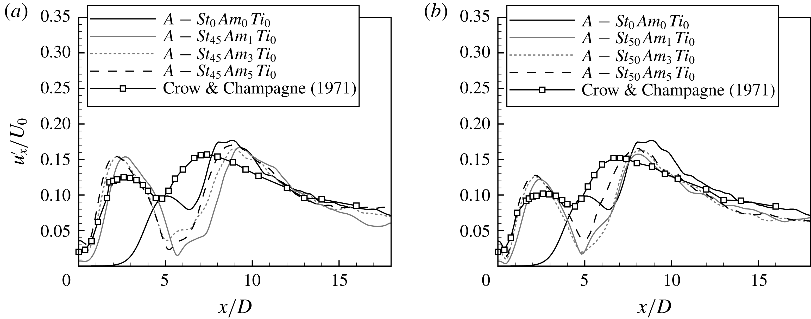
According to the experimental data of Crow & Champagne (Reference Crow and Champagne1971) a further increase of the forcing frequency leads to a decrease of the fluctuation level. The maximum of the fluctuating velocity for the forcing frequency
 $St_{D,e}=0.37$
was
 $0.21U_{0}$
(see figure 20). It can be readily seen from figure 24 that increasing the forcing frequency to
 $St_{D,e}=0.45$
and
 $St_{D,e}=0.5$
decreases the maximum to
 $0.15U_{0}$
and
 $0.1U_{0}$
, respectively. It should be stressed that the forcing frequency does not influence the distance of the maximum location from the inlet. The value of the maximum predicted numerically slightly overestimates experimental results but the tendency is perfectly reproduced.
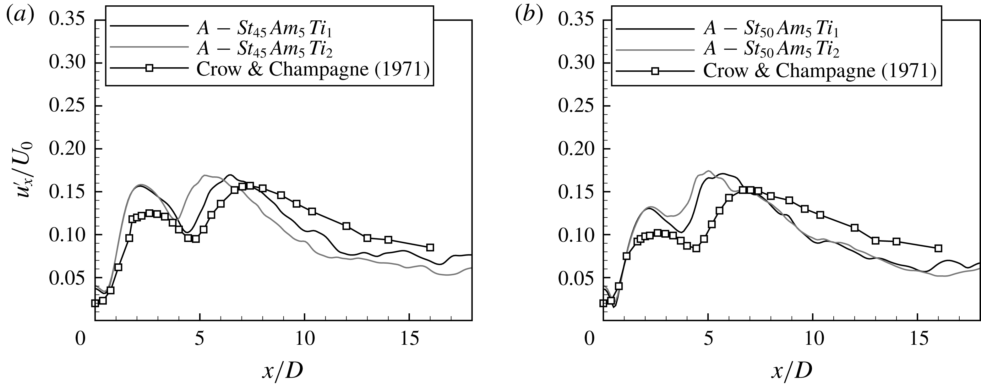
Figure 25 shows the results obtained with higher inlet turbulence level. Again, an agreement between the experimental data of Crow & Champagne (Reference Crow and Champagne1971) and the simulation results obtained for higher turbulence level is better than in the case of the lowest
 $Ti$
.
The highest frequency of the forcing used in the experiment of Crow & Champagne (Reference Crow and Champagne1971) corresponded to
 $St_{D,e}=0.5$
. Within the present numerical study a forcing with higher frequencies was also analysed. Increasing the stimulation frequency further above
 $St_{D,e}=0.5$
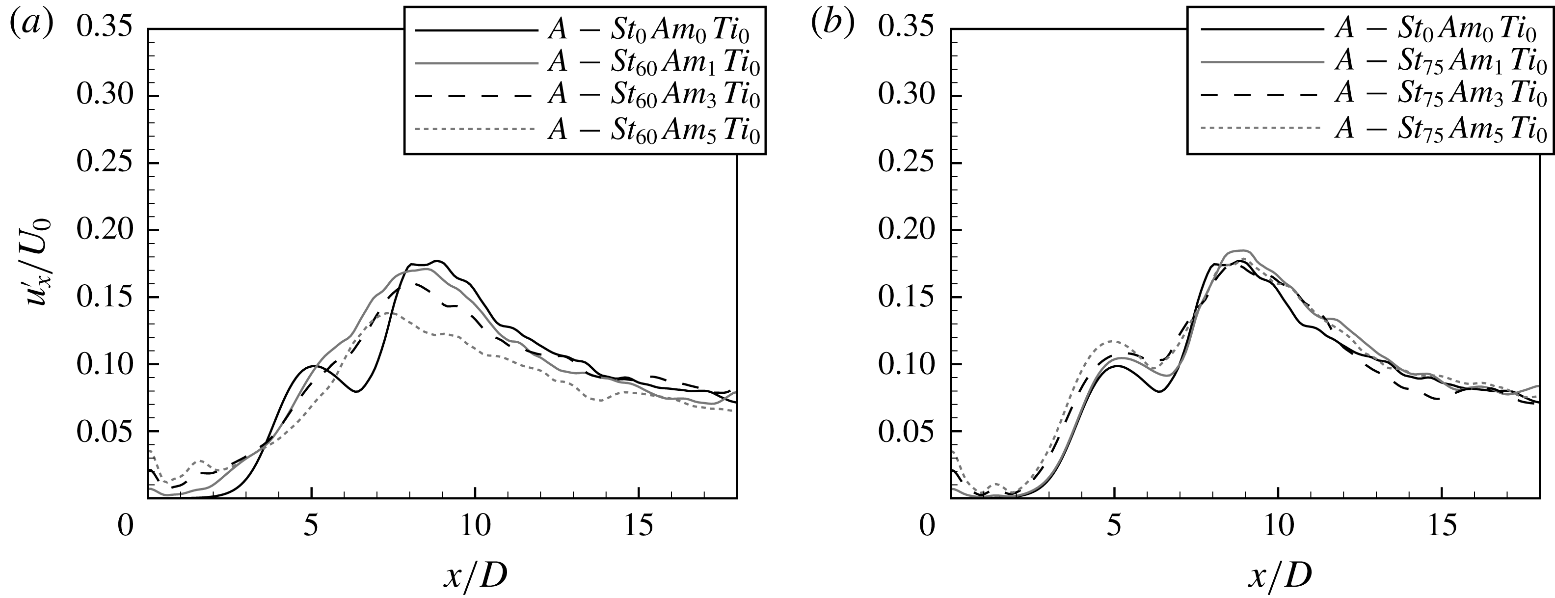
resulted in a weaker influence of the forcing on the flow field. The results for
 $St_{D,e}=0.6$
and
 $St_{D,e}=0.75$
are shown in figure 26. For frequencies higher than
 $St_{D,e}=0.7$
the mean (not shown in the paper) and fluctuating velocity profiles were practically independent of the external stimulation. Examples of such results are shown in figure 26(b) where the effects of stimulation with the non-dimensional frequency
 $St_{D,e}=0.75$
are illustrated. It can be readily seen that for the high frequency the perturbation imposed at the inlet is rapidly damped, no matter how large is the forcing amplitude, and finally the flow structure is very similar to that observed for the jet without any excitation.
Fluctuating velocity profiles. Test cases: (a)
 $A$
–
 $St_{0}Am_{0}Ti_{0}$
,
 $A$
–
 $St_{60}Am_{1}Ti_{0}$
,
 $A$
–
 $St_{60}Am_{3}Ti_{0}$
and
 $A$
–
 $St_{60}Am_{5}Ti_{0}$
; (b)
 $A$
–
 $St_{0}Am_{0}Ti_{0}$
,
 $A$
–
 $St_{75}Am_{1}Ti_{0}$
,
 $A$
–
 $St_{75}Am_{3}Ti_{0}$
and
 $A$
–
 $St_{75}Am_{5}Ti_{0}$
.

The independence of the flow structure from the stimulation with Strouhal number
 $St_{D,e}=0.75$
is also visible in the spectra shown in figure 27. The peak corresponding to the forcing frequency is visible only in the near-jet field at a distance
 $x/D\leqslant 3.3$
. Further downstream broadband oscillations with central frequency
 $St_{D}\approx 0.5$
dominate in exactly the same way as in the unexcited jet (see figure 2).
Knowing the jet response to the forcing with varying frequency and the striking similarity of the numerical and experimental results of Crow & Champagne (Reference Crow and Champagne1971), one could pose important questions: What is the frequency selection mechanism of the preferred mode? Why does the forcing with
 $St_{D,e}\approx 0.3$
lead to the highest increase of the fluctuations? For frequencies
 $St_{D,e}<0.3$
and increased turbulence level
 $Ti=1$
–
 $2\,\%$
the jet response to the external forcing is very weak, as found in most experimental studies. Probably, initially amplified primary structures are distorted by turbulence and break up preventing vortex pairing. As a consequence, the fluctuation level remains as in the natural jet. Increasing the forcing frequency leads to an amplification of the primary structures with a shorter wavelength. The shorter distance between the primary structures provokes interactions. As a consequence, larger and stronger structures which are more resistant to the turbulent fluctuations are generated. These structures could develop at a longer distance leading to higher level of fluctuations. A critical frequency was
 $St_{D,e}\approx 0.3$
. However, this could be dependent on the turbulence intensity at the nozzle exit. Further increase of the forcing frequency leads to a shorter distance between the primary structures which interact being not fully developed. This means that in the case of the preferred mode the primary structures develop as the Kelvin–Helmholtz instability and then the nonlinear interactions control the size of the structures. Hence, the frequency selection mechanism depends on the nonlinear interactions of primary unstable structures. However, a relation between the Kelvin–Helmholtz instability and the preferred mode is certainly not fully understood. In the calculations described above, due to the chosen shear-layer thickness, the natural frequency of the Kelvin–Helmholtz instability was close to the frequency of the preferred mode. In such a case these two modes are coupled, and hence the forcing with frequency close to the preferred mode amplifies also the shear-layer mode. In view of the results presented, the following questions can be formulated: (i) Could the preferred mode be triggered when the natural shear-layer mode frequency is far from the preferred mode frequency, for example when the shear layer is very thin? (ii) Could the preferred mode be triggered in a fully turbulent shear layer? Following the opinion expressed by Hussain & Zaman (Reference Hussain and Zaman1981), a sufficiently high external forcing can always produce a structure that is infrequent in the natural flow. It seems that in such cases the preferred mode could also be triggered independently of the Kelvin–Helmholtz instability but the subsequent preferred frequency selection mechanism should be the same as described above.
Evolution of spectra of axial velocity fluctuations. Test case:
 $A$
–
 $St_{75}Am_{5}Ti_{0}$
.

3.3 Excited jets: test cases with
$R/\unicode[STIX]{x1D703}=28$

Analogous calculations were performed for the jet with the thinner shear layer characterized by the parameter
 $R/\unicode[STIX]{x1D703}=28$
and the low turbulence level
 $Ti=0.01\,\%$
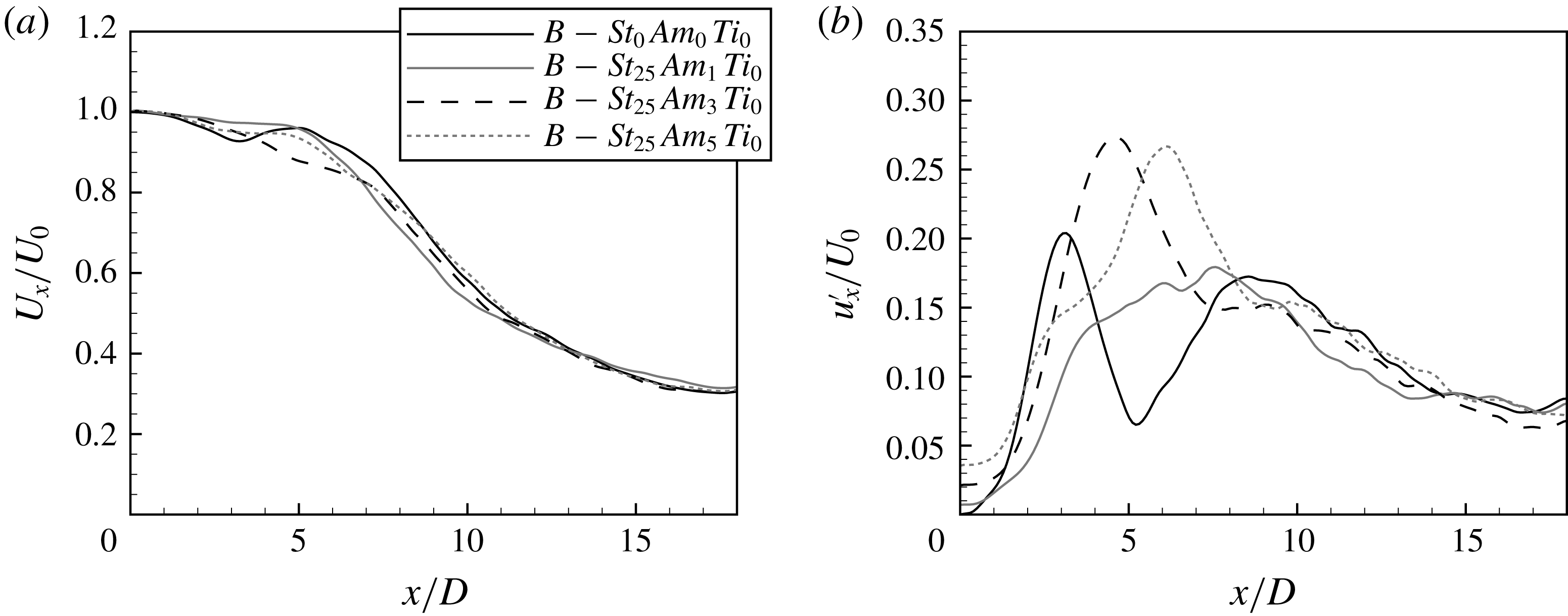
for which the self-sustained oscillations were identified by Boguslawski et al. (Reference Boguslawski, Tyliszczak, Drobniak and Asendrych2013) and Wawrzak et al. (Reference Wawrzak, Boguslawski and Tyliszczak2015). Figure 28 shows the mean and fluctuating velocity profiles for the forced jet with non-dimensional frequency
 $St_{D,e}=0.25$
and varying amplitude. It can be seen that for the weakest forcing with
 $Am=1\,\%$
the fluctuations are damped in contrast to the results obtained for the jet with shear layer
 $R/\unicode[STIX]{x1D703}=16$
shown in figure 8. Increasing further the forcing amplitude led to an increased level of the fluctuations compared to the natural self-sustained regime but slightly lower than in the case
 $R/\unicode[STIX]{x1D703}=16$
. Moreover, increasing the amplitude from
 $Am=3\,\%$
to
 $5\,\%$
does not amplify the oscillations and only shifts the maximum of the fluctuations slightly downstream. Hence, the jet response depends significantly on the shear-layer thickness. The changes in the fluctuations are reflected in the mean velocity profiles. In the case of the self-sustained mode without forcing the local minimum of the mean velocity profile at a distance
 $x/D\approx 3$
corresponds to the maximum of fluctuations. In the forced jet this minimum does not occur.
(a) Mean and (b) fluctuating velocity profiles. Test cases:
 $B$
–
 $St_{0}Am_{0}Ti_{0}$
,
 $B$
–
 $St_{25}Am_{1}Ti_{0}$
,
 $B$
–
 $St_{25}Am_{3}Ti_{0}$
and
 $B$
–
 $St_{25}Am_{5}Ti_{0}$
.

More information on the mechanism of the jet response can be found in the spectra of the axial velocity shown in figure 29. Close to the inlet at a distance
 $x/D\approx 1$
two peaks are visible, one corresponding to the forcing frequency
 $St_{D,e}=0.25$
and the other corresponding to the self-sustained mode
 $St_{D}=0.75$
. Further downstream the harmonics of the forcing frequency and subharmonic of the self-sustained mode develop indicating the vortex pairing process. Such a spectrum manifests the presence of two distinct modes and their mutual interactions.
Evolution of spectra of axial velocity fluctuations. Test case:
 $B$
–
 $St_{25}Am_{1}Ti_{0}$
.

By contrast, in the spectra obtained for the strongest forcing with amplitude
 $Am=5\,\%$
, presented in figure 30, the traces of the natural self-sustained mode are visible only in the vicinity of the nozzle exit. Further downstream only the component related to the forcing with frequency
 $St_{D,e}=0.25$
dominates.
Evolution of spectra of axial velocity fluctuations. Test case:
 $B$
–
 $St_{25}Am_{5}Ti_{0}$
.

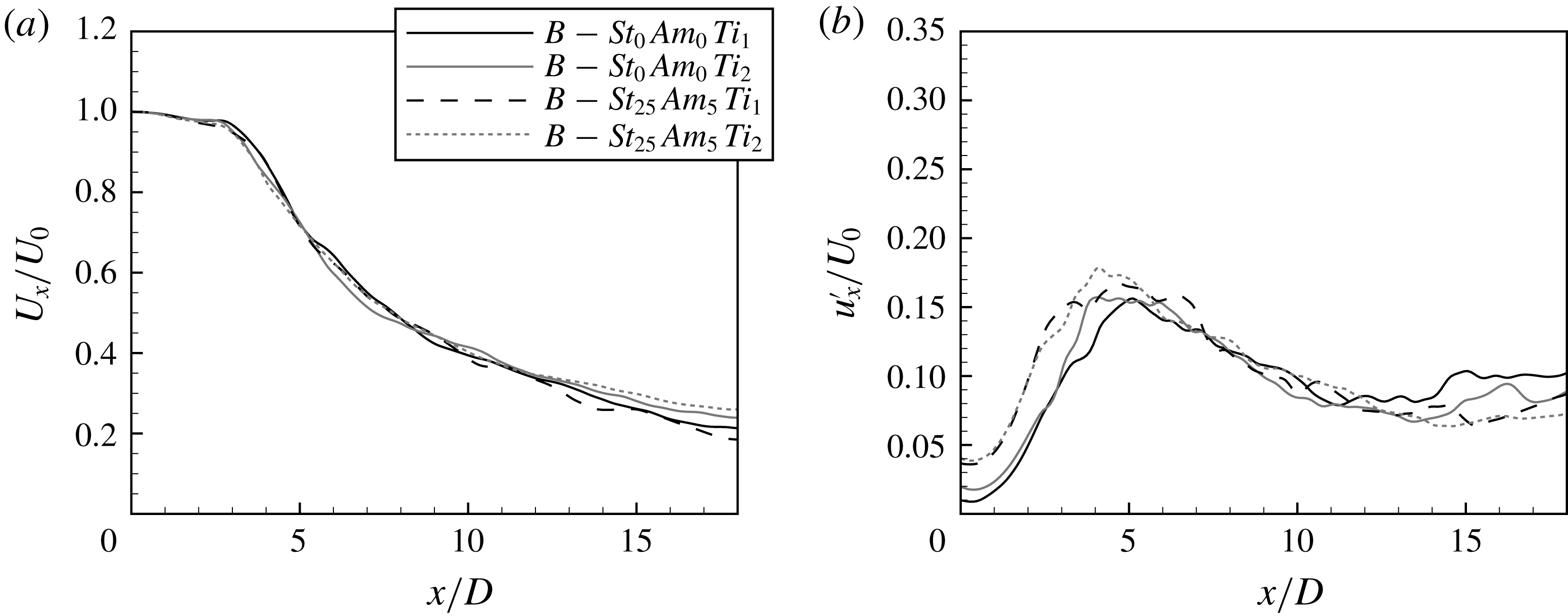
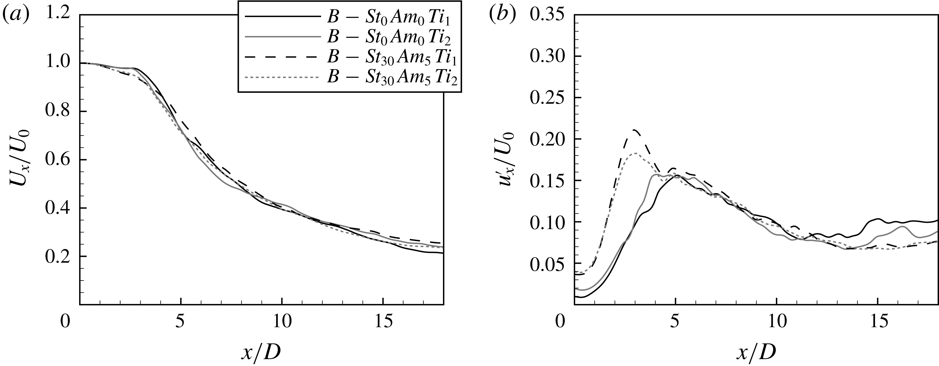
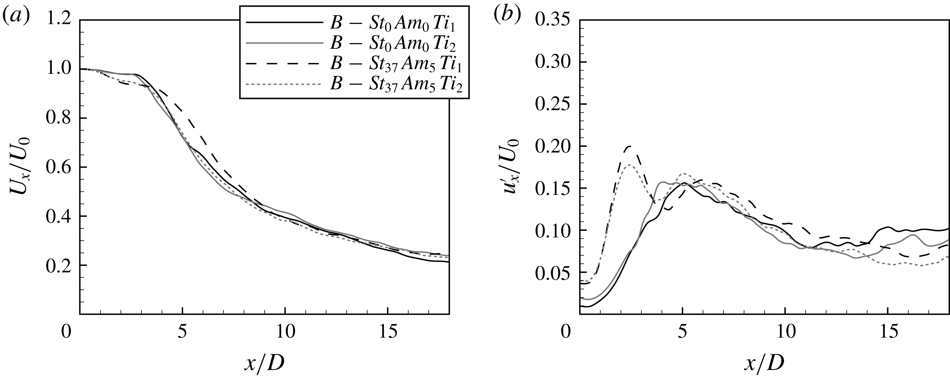
Figure 31 shows the jet response to the forcing in the case of increased turbulence intensity. It is seen that the forcing does not change the mean velocity profile and only weakly affects the fluctuation level. The maximum of the fluctuating velocity occurs at a distance
 $x/D=4$
–
 $5$
and attains a level
 $0.15U_{0}$
–
 $0.17U_{0}$
. It depends more on the inlet turbulence than on the forcing. The results are similar to those obtained for
 $R/\unicode[STIX]{x1D703}=16$
shown in figure 13.
(a) Mean and (b) fluctuating velocity profiles. Test cases:
 $B$
–
 $St_{0}Am_{0}Ti_{1}$
,
 $B$
–
 $St_{0}Am_{0}Ti_{2}$
,
 $B$
–
 $St_{25}Am_{5}Ti_{1}$
and
 $B$
–
 $St_{25}Am_{5}Ti_{2}$
.

A slight increase of the forcing frequency to
 $St_{D,e}=0.3$
significantly changes the jet response as shown in figure 32. In this case even the forcing with amplitude
 $Am=3\,\%$
does not amplify the flow oscillations. Only the forcing with
 $Am=5\,\%$
amplifies the jet oscillations. It is worth noting that the minimum at the mean velocity profile at
 $x/D\approx 3$
is visible in the cases of the the natural jet and the jet with forcing
 $Am=5\,\%$
, while for amplitudes
 $Am=1\,\%$
and
 $3\,\%$
this minimum disappears.
(a) Mean and (b) fluctuating velocity profiles. Test cases:
 $B$
–
 $St_{0}Am_{0}Ti_{0}$
,
 $B$
–
 $St_{30}Am_{1}Ti_{0}$
,
 $B$
–
 $St_{30}Am_{3}Ti_{0}$
and
 $B$
–
 $St_{30}Am_{5}Ti_{0}$
.

The spectra shown in figure 33 reveal many components related to the forcing frequency
 $St_{D,e}=0.3$
, its harmonic and the self-sustained mode
 $St_{D}=0.75$
along with its subharmonic. Both modes are present up to a distance
 $x/D=3.3$
showing a complex interaction of two different types of jet instability.
Evolution of spectra of axial velocity fluctuations. Test case:
 $B$
–
 $St_{30}Am_{3}Ti_{0}$
.

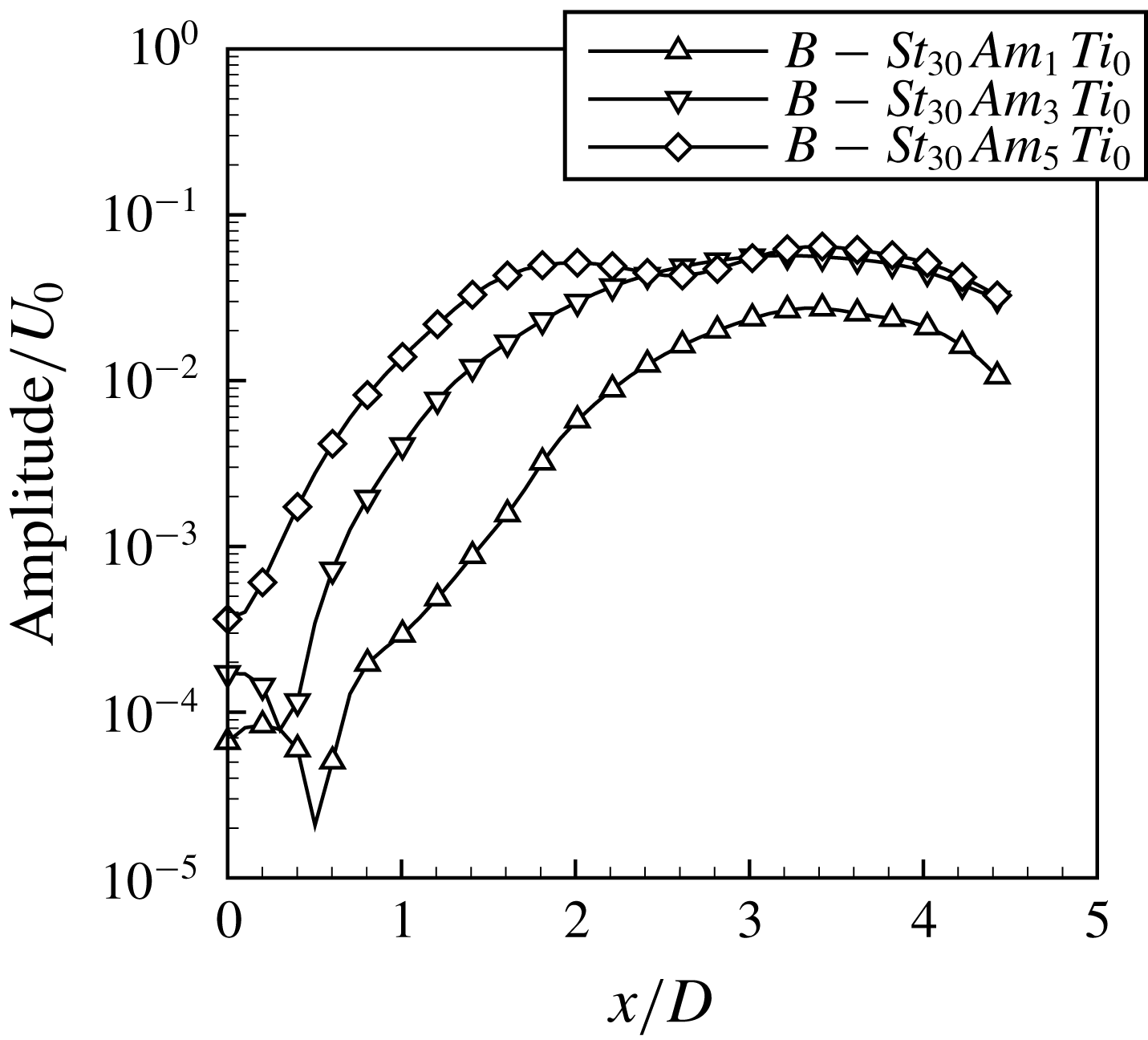
Figure 34 shows the evolution of the amplitude of the mode
 $St_{D}=0.6$
. It can be seen that for the forcing with
 $Am=1\,\%$
and
 $3\,\%$
the fluctuations are initially damped and then grow up to a distance
 $x/D=2$
–
 $3$
. For the case with
 $Am=5\,\%$
this mode grows starting already from the inlet.
Amplitude evolution of the mode
 $St_{D}=0.6$
. Test cases:
 $B$
–
 $St_{30}Am_{1}Ti_{0}$
,
 $B$
–
 $St_{30}Am_{3}Ti_{0}$
and
 $B$
–
 $St_{30}Am_{5}Ti_{0}$
.

Forcing the jet with frequency
 $St_{D,e}=0.3$
and amplitude
 $Am=5\,\%$
leads to an increased level of fluctuations also in the case of a higher turbulence intensity
 $Ti=1\,\%$
and
 $2\,\%$
as shown in figure 35. Increased fluctuations in the forced jet are also reflected in the mean velocity profiles by shortened potential core. However, the local minimum which is typical for the self-sustained mode is not observed.
(a) Mean and (b) fluctuating velocity profiles. Test cases:
 $B$
–
 $St_{0}Am_{0}Ti_{1}$
,
 $B$
–
 $St_{0}Am_{0}Ti_{2}$
,
 $B$
–
 $St_{30}Am_{5}Ti_{1}$
and
 $B$
–
 $St_{30}Am_{5}Ti_{2}$
.

Choosing the forcing frequency equal to the subharmonic of the self-sustained regime
 $St_{D,e}=0.37$
does not affect the level of fluctuations, as shown in figure 36. The only effect of the excitation is a slight shift of the maximum of the fluctuations upstream with increasing amplitude of forcing. Its influence on the mean velocity in the near field for
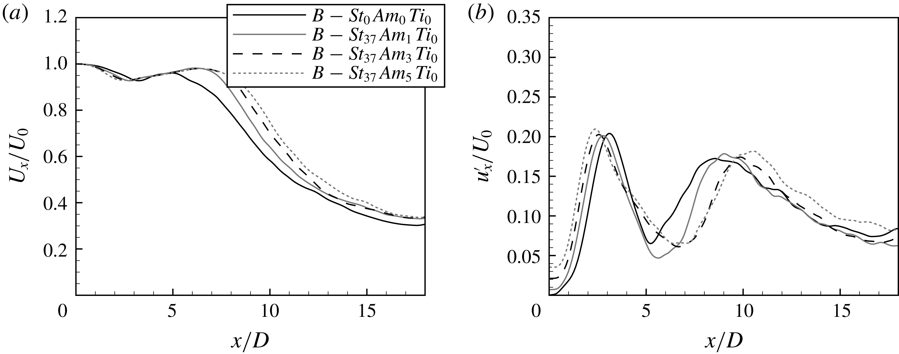
 $x/D<5$
is also very weak and only further downstream are some more differences visible. For the higher forcing amplitude the mean velocity decay starts later.
(a) Mean and (b) fluctuating velocity profiles. Test cases:
 $B$
–
 $St_{0}Am_{0}Ti_{0}$
,
 $B$
–
 $St_{37}Am_{1}Ti_{0}$
,
 $B$
–
 $St_{37}Am_{3}Ti_{0}$
and
 $B$
–
 $St_{37}Am_{5}Ti_{0}$
.

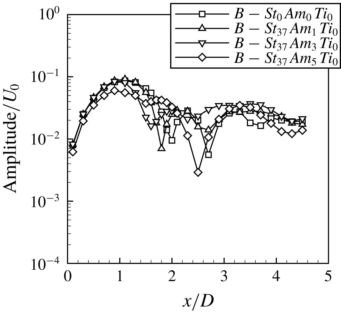
Figure 37 shows the evolution of the amplitude of the mode
 $St_{D}=0.75$
. It can be seen that the jet is in the self-sustained regime and the external stimulation does not change this regime. Comparing the results shown in figure 37 with the results obtained for the jet with
 $R/\unicode[STIX]{x1D703}=16$
with the same forcing parameters (see figure 22) it could be seen that the level of the amplitude of the mode
 $St_{D}=0.75$
is for the present case one order of magnitude higher. That means that previously for
 $R/\unicode[STIX]{x1D703}=16$
the forcing was not able to introduce the jet into the self-sustained regime despite that the primary structures interacted at a distance
 $x/D=1$
.
Amplitude evolution of the mode
 $St_{D}=0.75$
. Test cases:
 $B$
–
 $St_{0}Am_{0}Ti_{0}$
,
 $B$
–
 $St_{37}Am_{1}Ti_{0}$
,
 $B$
–
 $St_{37}Am_{3}Ti_{0}$
and
 $B$
–
 $St_{37}Am_{5}Ti_{0}$
.

The jet response to the forcing
 $St_{D,e}=0.37$
in the case of higher inlet turbulence
 $Ti=1\,\%$
and
 $2\,\%$
is shown in figure 38. The forcing influence in this case is very similar to the forcing with
 $St_{D,e}=0.3$
shown in figure 35 concerning both the mean and fluctuating velocity profiles.
(a) Mean and (b) fluctuating velocity profiles. Test cases:
 $B$
–
 $St_{0}Am_{0}Ti_{1}$
,
 $B$
–
 $St_{0}Am_{0}Ti_{2}$
,
 $B$
–
 $St_{37}Am_{5}Ti_{1}$
and
 $B$
–
 $St_{37}Am_{5}Ti_{2}$
.

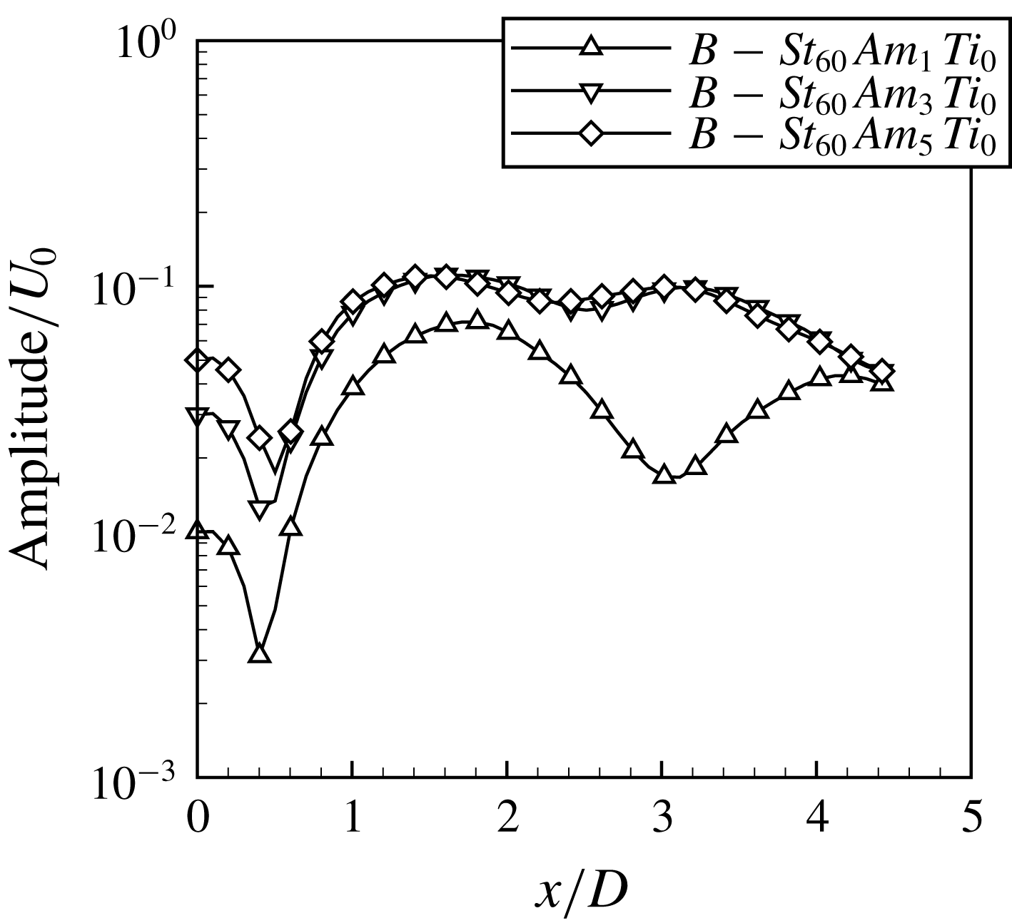
Increasing further the forcing frequency to
 $St_{D,e}=0.6$
that is off the natural frequency of the self-sustained mode leads to a jet response similar to that observed for the forcing frequencies
 $St_{D,e}=0.25$
and
 $0.3$
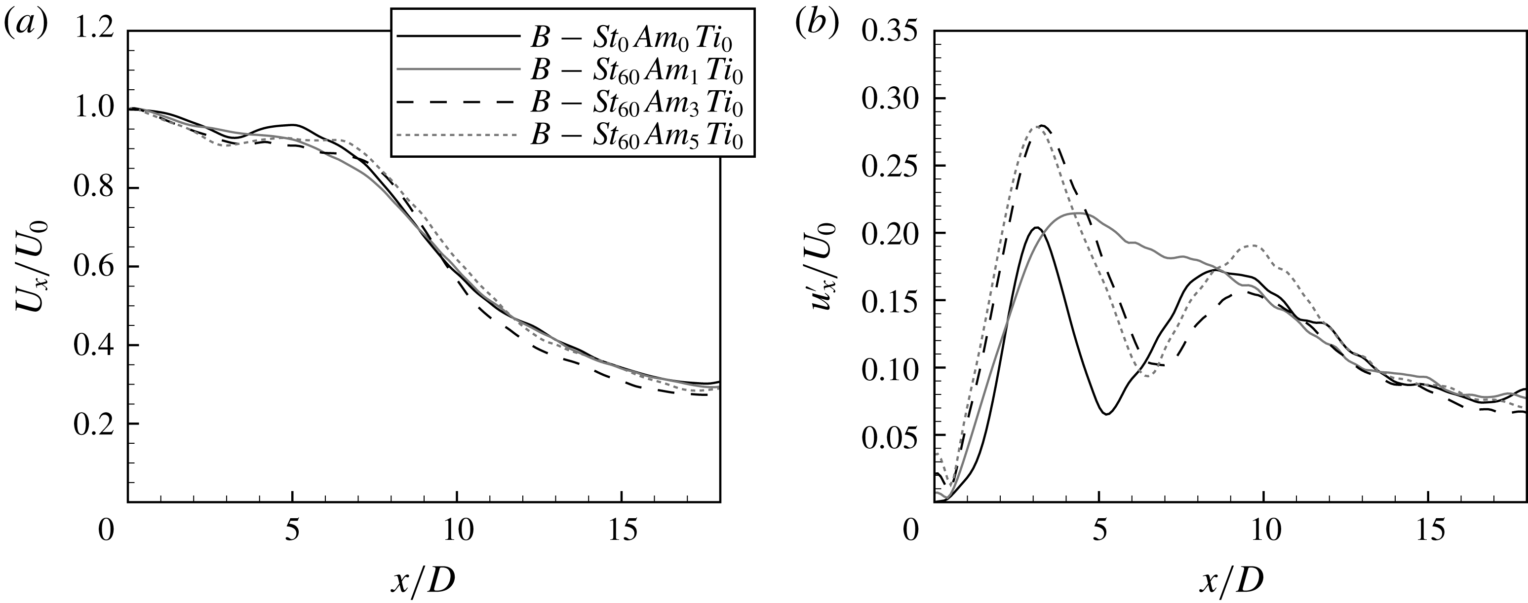
. Figure 39 shows the mean and fluctuating velocity profiles for this case. It is seen again that a weak excitation disturbs the natural oscillations but does not amplify the fluctuation level. However, as observed also in the case of the thicker shear layer, the higher frequency oscillations are damped at a short distance. It is worth noting here that in the case of
 $R/\unicode[STIX]{x1D703}=28$
and forcing
 $St_{D,e}=0.6$
for which the solutions are shown in figure 39 the jet response is significantly different from that observed for
 $R/\unicode[STIX]{x1D703}=16$
(see figure 26
a). For the thicker shear layer the level of fluctuations under forcing is lower than for the unexcited jet while in the case of thinner shear layer a certain increase of the fluctuation level is observed.
(a) Mean and (b) fluctuating velocity profiles. Test cases:
 $B$
–
 $St_{0}Am_{0}Ti_{0}$
,
 $B$
–
 $St_{60}Am_{1}Ti_{0}$
,
 $B$
–
 $St_{60}Am_{3}Ti_{0}$
and
 $B$
–
 $St_{60}Am_{5}Ti_{0}$
.

The influence of the forcing with frequency
 $St_{D,e}=0.6$
on the fluctuating velocity profile for the thin shear layer
 $R/\unicode[STIX]{x1D703}=28$
seems to be similar to the influence of the forcing with frequency
 $St_{D,e}=0.3$
. However, looking at the evolution of the amplitude of the mode
 $St_{D}=0.6$
, shown in figure 40, qualitative differences are observed compared to the results shown in figure 34. It can be seen that the weakest forcing disturbs the self-sustained oscillations without an increase of the fluctuation level. A higher forcing amplitude leads to an increased fluctuation level. Moreover, further increase of the forcing does not change the jet dynamics suggesting that in this case the jet is again in the self-sustained mode but with slightly higher amplitude. It should be noted here that in the experiment of Zaman & Hussain (Reference Zaman and Hussain1980) it was shown that the highest jet response is obtained for a forcing frequency higher than that of the preferred mode measured by Crow & Champagne (Reference Crow and Champagne1971).
Amplitude evolution of the mode
 $St_{D}=0.6$
. Test cases:
 $B$
–
 $St_{60}Am_{1}Ti_{0}$
,
 $B$
–
 $St_{60}Am_{3}Ti_{0}$
and
 $B$
–
 $St_{60}Am_{5}Ti_{0}$
.

Forcing the jet with a frequency equal to the frequency of the self-sustained mode
 $St_{D,e}=0.75$
, not shown here, again has no effect on the jet dynamics.
One could conclude that forcing the jet in the self-sustained regime with the frequency of the natural oscillations or its subharmonics has nearly no effect on the jet dynamics confirming that the flow oscillations are ‘saturated’ by nonlinear interactions. Forcing the jet with a frequency off the natural jet oscillations could lead to twofold effects. A weak forcing disturbs the self-sustained mode and reveals a complex mechanism of interactions of two different modes, one related to natural flow oscillations and the other caused by the excitation. In such a case the level of the flow fluctuations is not increased. On increasing the forcing amplitude it could be seen that the oscillations were amplified compared to the natural self-sustained jet. However, it seems that depending on the forcing frequency different mechanisms of this amplification are revealed.
4 Concluding remarks
The paper presents numerical studies using the LES approach of a round free jet stimulated with an external varicose excitation. A motivation for these studies was previous experimental and numerical investigations presented by Boguslawski et al. (Reference Boguslawski, Tyliszczak, Drobniak and Asendrych2013) that identified a new transition regime in a round jet. This regime, called the self-sustained regime, is triggered in a free jet when the shear-layer thickness at the nozzle exit is sufficiently thin under conditions of a low turbulence level. The mean and fluctuating velocity profiles registered in the jet being in the self-sustained mode show striking similarities to the statistics registered in jets stimulated by external forcing with the frequency of the preferred mode. Within the present studies jets with two different shear-layer thicknesses were analysed numerically. In the case of the thicker shear layer characterized by the parameter
 $R/\unicode[STIX]{x1D703}=16$
the self-sustained oscillations were not triggered. The stimulation of the jet with frequency equal to the natural flow oscillations, generated by the Kelvin–Helmholtz instability, resulted in an amplification of the fluctuations growing monotonically with the stimulation amplitude. In this case certainly one deals with an amplification of naturally present vortices and the jet response could be classified as an ‘amplifier’. However, a slight shift of the forcing frequency closer to the subharmonic of the frequency characteristic to the self-sustained mode alters the jet response markedly. Even a very weak external perturbation modifies qualitatively the profile of the fluctuating velocity along the jet axis marking a change in the transition regime. Moreover, in this case the fluctuating velocity profile is quite similar to the one obtained for a thin shear layer when the jet is in the natural self-sustained regime and to the fluctuation profiles observed in the experiment of Crow & Champagne (Reference Crow and Champagne1971) when the preferred mode was present. A deeper analysis of the flow structure performed using the
 $Q$
-parameter iso-contours and evolution of the amplitude of the amplified mode showed that in the case of
 $R/\unicode[STIX]{x1D703}=16$
the self-sustained regime was not triggered. However, when the forcing frequency is close to the preferred mode the primary structures interacted at a short distance from the nozzle exit forming larger and stronger vortical structures. If the vortex pairing is not present sufficiently close to the nozzle exit the turbulent fluctuations can distort the primary vortices leading to a weak response of the jet to the external forcing. Hence, the jet response to the external forcing and frequency selection mechanism seem to be determined by a character of the nonlinear interaction of the primary flow structures. Further increase of the forcing frequency leads to a decreased level of fluctuations that is in excellent agreement with the results of Crow & Champagne (Reference Crow and Champagne1971). It is worth stressing that Crow & Champagne (Reference Crow and Champagne1971) at the early stage of the preferred mode investigations already suggested that the frequency selection mechanism is established as a result of the nonlinear interactions.
The computations performed for the jet with
 $R/\unicode[STIX]{x1D703}=28$
, i.e. in the natural self-sustained mode, revealed that in this case the jet response seemed to be quite different from that in the cases characterized by
 $R/\unicode[STIX]{x1D703}=16$
. This shows that the jet response to the external forcing is a complex phenomenon and its interpretation requires precise knowledge of the flow conditions at the nozzle exit including the shear-layer thickness and turbulence intensity. The present results could explain the differences in the experimental results of Crow & Champagne (Reference Crow and Champagne1971) and Zaman & Hussain (Reference Zaman and Hussain1980). It can be concluded that forcing with frequency equal to the frequency of the natural self-sustained mode or with its subharmonic has practically no effect on the jet dynamics. The jet response to forcing with frequencies different from the natural one depends on the forcing amplitude. A weak forcing disturbs the self-sustained mode leading to interaction with the vortices triggered by forcing. A stronger forcing suppresses the self-sustained mode and only the frequency components related to the stimulation are observed in the spectra. However, it must be stressed that a mechanism responsible for the jet response to an external forcing under the self-sustained regime has not been extensively studied so far and a full understanding of this phenomenon needs further studies and careful analysis.
Acknowledgements
The research was supported by the Polish National Science Centre, project no. 2016/21/B/ST8/00414. The computations were carried out using PL-Grid Infrastructure. The authors are grateful to Professor Lutz Lesshafft whose valuable suggestions stimulated the current investigations.