Spatial organisation of velocity structures for large passive scalar gradients

Angeliki Laskari; T. Saxton-Fox; B. J. McKeon

doi:10.1017/jfm.2019.977

Spatial organisation of velocity structures for large passive scalar gradients

Published online by Cambridge University Press: 06 January 2020

and

Angeliki Laskari*: Affiliation:
Graduate Aerospace Laboratories, California Institute of Technology, Pasadena, CA 91106, USA
T. Saxton-Fox: Affiliation:
Department of Aerospace Engineering, University of Illinois, Urbana, IL 61801, USA
B. J. McKeon: Affiliation:
Graduate Aerospace Laboratories, California Institute of Technology, Pasadena, CA 91106, USA
*: †Email address for correspondence: alaska@caltech.edu

Article contents

Abstract
Introduction
Methodology
Results
Time scales of large MP deflections
Discussion
Conclusions
References

Rights & Permissions

Abstract

Velocity structures associated with large streamwise density gradients in an incompressible turbulent boundary layer (with air as the working fluid, $Pr=0.71$) are analysed experimentally using planar image velocimetry and aero-optic measurements. The resulting flow topologies for the velocity fluctuations associated with large negative and positive density gradients are in excellent agreement with results for coolings and heatings in time, respectively (Antonia & Fulachier, J. Fluid Mech., vol. 198, 1989, pp. 429–451). The current results are complimentary to those from Saxton-Fox et al. (AIAA J., vol. 57 (7), 2019, pp. 2828–2839), on the signature of the vertical velocity structures associated with large density gradients. In the present work, these structures are shown to exhibit a sign change, consistent with the scalar gradient, and are localised in the wall-normal direction with an average height of approximately $0.1\unicode[STIX]{x1D6FF}$, almost constant for increasing distance from the wall. The corresponding small-scale streamwise fluctuations also exhibit a consistent sign change, which is found to originate, on average, from upstream leaning structures. The emerging picture for the velocity field is then that of a multiscale phenomenon, where small-scale structures, responsible for large optical aberrations, are superimposed on the back of large-scale bulge-like structures that are known to populate the outer layers. The proposed conceptual model is consistent with early ideas of ‘typical’ eddies (Falco, Phys. Fluids, vol. 20 (10), 1977, pp. S124–S132), the hairpin vortex model and associated shear layers (Adrian et al., J. Fluid Mech., vol. 422, 2000, pp.1–54), as well as with notions of multiscale velocity organisation in shear layers (Klewicki & Hirschi, Phys. Fluids, vol. 16 (11), 2004, pp. 4163–4176; Saxton-Fox et al. 2019), and it provides new insight into the geometry of the small-scale velocity structures.

JFM classification

Boundary Layers: Boundary layer structure Turbulent Flows: Turbulent boundary layers

Information

Type: JFM Papers
Information: Journal of Fluid Mechanics , Volume 885 , 25 February 2020, A33
DOI: https://doi.org/10.1017/jfm.2019.977 [Opens in a new window]
Copyright: © 2020 Cambridge University Press

1 Introduction

The structural organisation of turbulent boundary layers has been an important topic of research in fluid dynamics for several decades. Out of the many features of organised motion observed throughout the boundary layer, large-scale velocity structures populating the logarithmic and wake regions are of particular interest due to the amount of kinetic energy and Reynolds stress they have been recently shown to carry (Guala, Hommema & Adrian (Reference Guala, Hommema and Adrian2006) and Balakumar & Adrian (Reference Balakumar and Adrian2007) among others), as well as their modulating effect on the near-wall cycle (Hutchins & Marusic Reference Hutchins and Marusic2007; Mathis, Hutchins & Marusic Reference Mathis, Hutchins and Marusic2009). The connection of these velocity structures with vortical structures and shear layers in the logarithmic region (Lozano-Duran, Flores & Jimenez Reference Lozano-Duran, Flores and Jimenez2012; de Silva et al. Reference de Silva, Philip, Hutchins and Marusic2017) and with the bulge-like nature of the free-stream boundary (see for example Falco Reference Falco1977; Adrian, Meinhart & Tomkins Reference Adrian, Meinhart and Tomkins2000; de Silva et al. Reference de Silva, Kevin, Baidya, Hutchins and Marusic2018) are points of ongoing research and various techniques have been employed for their investigation.

Earlier studies on this subject, lacking the spatial and temporal information that direct numerical simulations (DNS) and advanced experimental techniques can provide at present, employed passive scalar tracers to gain more insight into the structuring of the boundary layer. Falco (Reference Falco1977) used smoke as a passive scalar contaminant together with hot-wire measurements to analyse the link between small eddy motions (‘typical eddies’) – associated with the bursting mechanism – and large-scale motions in the outer region of a boundary layer. Chen & Blackwelder (Reference Chen and Blackwelder1978) used a moderately heated wall to introduce temperature as a passive scalar in a turbulent boundary layer flow, which allowed the identification of an inclined sharp temperature front, extending across the entire boundary layer height. The authors showed that the temperature gradient was linked to the backs of the turbulent bulges in the turbulent/non-turbulent (TNTI) interface, while within the turbulent region it was associated with an internal shear layer and the bursting phenomenon near the wall. Similar temperature ramps were also found in the atmospheric surface layer (Antonia et al. Reference Antonia, Chambers, Friehe and Van Atta1979) indicating the presence of organised large-scale motion. Following these observations, several studies used simple ramp models for the large-scale motion to explain the non-zero odd-structure functions and moments of temperature (skewness in particular), which represent a departure from the concept of local isotropy (Gibson, Friehe & McConnell Reference Gibson, Friehe and McConnell1977; Sreenivasan & Antonia Reference Sreenivasan and Antonia1977; Antonia & Van Atta Reference Antonia and Van Atta1978, Reference Antonia and Van Atta1979).

The fast advancement of both numerical and experimental tools in the years that followed led to the development of different conceptual models for the structural organisation in boundary layers, of which the hairpin model (Head & Bandyopadhyay (Reference Head and Bandyopadhyay1981) supporting the early model of Theodorsen (Reference Theodorsen1952)) was one of the most prominent. As such, subsequent studies tried to incorporate it into the existing observations about large-scale coherent motion. Antonia et al. (Reference Antonia, Fulachier, Krishnamoorthy, Benabid and Anselmet1988a) used heat and dye as passive contaminants in air and water respectively and their results provided support for the connection between the inner and outer regions of the boundary layer through the temperature fronts (termed ‘coolings’) as suggested by Chen & Blackwelder (Reference Chen and Blackwelder1978). The authors also identified the importance of positive temperature gradients in the flow dynamics (‘heatings’, following earlier observations from Subramanian et al. (Reference Subramanian, Rajagopalan, Antonia and Chambers1982)) and made some comparisons between both heatings and coolings and the hairpin model, acknowledging, however, that visual information was not enough to draw a direct link between these features. Partial support for this association was presented in Antonia & Fulachier (Reference Antonia and Fulachier1989), albeit still limited due to the missing spanwise information. More interestingly, the authors could identify the connection of heatings and coolings with the flow topology and showed that the former go through unstable foci, while the latter are aligned with diverging separatrices going through saddle points and are associated with larger spanwise vorticity and strain rates. Similar observations were also made by Bisset, Antonia & Raupach (Reference Bisset, Antonia and Raupach1991), this time in a slightly heated rough-wall turbulent boundary layer. Further experimental evidence of the correlation between coherent structures and scalar transport was provided by the work of Vanderwel & Tavoularis (Reference Vanderwel and Tavoularis2016), who used concurrent stereo particle image velocimetry (PIV) and planar laser-induced fluorescence (PLIF) to analyse passive scalar dispersion; their results indicated strong correlation between the presence of hairpin vortices and large scalar flux and Reynolds stress events.

In terms of the dynamics and mixing of the scalar itself as well as its relationship with the three velocity components, Fulachier & Dumas (Reference Fulachier and Dumas1976) investigated the connection between velocity and scalar statistics in the case of a rough-wall boundary layer using heat as the passive contaminant. They showed that, except for the region very close to the wall, the temperature spectrum differs significantly from the streamwise velocity one and is shifted to higher frequencies. A better spectral analogy is achieved when a velocity spectrum defined as the sum of all velocity components and weighted by their variances is used (Fulachier & Dumas Reference Fulachier and Dumas1976). The close correlation between the streamwise velocity and temperature near the wall was further investigated by Antonia, Krishnamoorthy & Fulachier (Reference Antonia, Krishnamoorthy and Fulachier1988b), in particular regarding streak formation. They found that the wall region is populated with high-temperature low-speed streaks; however, the low-temperature high-speed streaks are the largest contributors in the longitudinal heat flux. Similar analyses were also significantly facilitated by the development of DNS in later years that allowed for derivative and spectral correlations (Kim & Moin (Reference Kim and Moin1989), Abe, Antonia & Kawamura (Reference Abe, Antonia and Kawamura2009), Antonia, Abe & Kawamura (Reference Antonia, Abe and Kawamura2009) and Li et al. (Reference Li, Schlatter, Brandt and Henningson2009) among others).

Despite this rapid development of DNS as well as of state-of-the-art experimental techniques for scalar measurements (such as PLIF), complete information of velocity and scalar fields is still limited to low Reynolds numbers in simulations and to low temporal and spatial resolution in experiments (where full-field three-dimensional scalar information is also a rarity). Even in cases where such datasets are available, they come at a very high computational and experimental cost and as such, methods that can still provide vital information with sparser inputs, and therefore at a lower cost, are of particular importance. Such an alternative was developed in the field of aero-optics and was initially applied to compressible flows, with the purpose of improving airborne optical systems (Gordeyev et al. Reference Gordeyev, Jumper, Ng and Cain2003). It is based on the fact that changes in density due to compressibility lead to a continuous variation in the index of refraction within a flow, which in turn leads to optical aberrations for linear wave fronts passing through the flow. Malley, Sutton & Kincheloe (Reference Malley, Sutton and Kincheloe1992) presented the development of an optical set-up to measure such aberrations for small-aperture beams, referred to as Malley probe (MP), which was then later extended to provide accurate measurements of optical length distortions in a variety of compressible flow configurations (Gordeyev, Hayden & Jumper (Reference Gordeyev, Hayden and Jumper2007) and Gordeyev et al. (Reference Gordeyev, Smith, Cress and Jumper2014) among others) including free shear layers, attached, and separated flows (Wang, Mani & Gordeyev Reference Wang, Mani and Gordeyev2012; Jumper & Gordeyev Reference Jumper and Gordeyev2017). Gordeyev et al. (Reference Gordeyev, Cress, Smith and Jumper2015) showed that a moderate increase of the wall temperature results in little or no change in turbulence statistics (heat acts as a passive scalar) but in an increase of density fluctuations in the boundary layer and a subsequent amplification of optical aberrations, thus extending the potential of aero-optic research to incompressible, low-speed flows. This was achieved by Smith et al. (Reference Smith, Gordeyev, Saxton-Fox and McKeon2014), who showed that the spectral characteristics of the beam deflection in an incompressible thermal boundary layer collapse with those from compressible flows under the appropriate normalisation. Following these observations, subsequent studies used the optical distortion as means to gain more information about the velocity and scalar fields, proposing an alternative approach to passive scalar measurements which requires a sparser input (integral measurements of the scalar gradients) and therefore a simpler and less expensive set-up, while still providing valuable information on the structural organisation of the flow (see Saxton-Fox et al. Reference Saxton-Fox, McKeon, Gordeyev and Smith2015; Gordeyev & Smith Reference Gordeyev and Smith2016). With respect to turbulent boundary layers that are of interest here, such information was shown to be pertinent for wake and logarithmic layer structures, since these are mainly responsible for the optical distortions measured (Wang & Wang Reference Wang and Wang2012).

Within this context, Saxton-Fox (Reference Saxton-Fox2018) employed a MP set-up to acquire integral measurements of streamwise density gradients in a mildly heated subsonic boundary layer, while simultaneous PIV measurements allowed for the identification of velocity structures conditioned on large density gradients; tall vertical velocity structures of opposing signs on either side of the MP beam, spanning from the wall up to the edge of the boundary layer, were found to be associated with large streamwise scalar gradients. The author postulated that these structures were a result of a wall-normal average of instantaneous smaller scales residing at the same streamwise location but at different heights $y$ from the wall, depending on the phase of large-scale streamwise velocity structures. This model was further developed in Saxton-Fox, McKeon & Gordeyev (Reference Saxton-Fox, McKeon and Gordeyev2019), where the effect of large-scale motion on the scalar statistics and the robust correlation of small-scale vertical velocity structures with the beam deflection sign were analysed and a conceptual picture of the spatial organisation of large and small scales responsible for the beam deflection was proposed. The purpose of the current work is to investigate and characterise, in an effort to separate in the wall-normal direction, the different vertical velocity scales triggering the large deflections of the optical beam, to identify the localised signatures of the corresponding streamwise velocity fluctuations and to synthesise the results into the broader current picture of the structure of turbulent boundary layers.

It should be noted here that, the use of the MP technique in aero-optical studies has mainly been geared towards the effects of turbulent structure on the aberrations of an incoming wave front. In this context, the correspondence between velocity and scalar fields is of the essence such that predictions can be made for the optical aberrations using information from the velocity field – which is generally easier to access. For compressible flows in particular, this analogy can be directly analysed using incompressible relations with appropriate scaling: Morkovin’s hypothesis and strong Reynolds analogy for adiabatic flows (see Morkovin (Reference Morkovin and Favre1962), Smits & Dussuage (Reference Smits and Dussuage2006) and Smith et al. (Reference Smith, Gordeyev, Saxton-Fox and McKeon2014) among others) and an extended Reynolds analogy for flows with a heat source similar to the case discussed in this work (see Gordeyev et al. Reference Gordeyev, Cress, Smith and Jumper2015). In incompressible passive scalar transport studies, where measurements or computations of scalar and velocity fields are acquired more easily, direct comparisons between the fields can be made and results have shown that a strong correlation exists between streamwise velocity and scalar fields, especially close to the wall and for molecular Prandtl numbers near unity (see for example Fulachier & Dumas Reference Fulachier and Dumas1976; Antonia & Van Atta Reference Antonia and Van Atta1978; Kim & Moin Reference Kim and Moin1989; Abe et al. Reference Abe, Antonia and Kawamura2009; Antonia et al. Reference Antonia, Abe and Kawamura2009; Li et al. Reference Li, Schlatter, Brandt and Henningson2009). However, as was mentioned above, full-field information for scalar transport in wall-bounded turbulent flows is still limited both experimentally and computationally; as such, in the present study we assess the amount of information that can be extracted about the flow when only limited information on the scalar is available. The aim is to exploit the integral measurements of the scalar gradient, as they were first employed in the aero-optics community, in order to analyse the velocity structures that are associated with extreme values of the gradient. The available information allows for very few – if any – assumptions regarding the scalar field itself; however, several comparisons with results from cold-wire studies on the flow topology and conditional structure can be made.

In the sections that follow, the experimental methods and flow analysis methods are presented, followed by results on the geometrical characteristics of conditionally averaged streamwise and wall-normal velocity fluctuations. Finally, a discussion on the conceptual ideas supported by these observations and a comparison with results from cold-wire studies are also presented.

2 Methodology

Throughout this paper, we use the coordinate system $x$, $y$ and $z$ to denote the streamwise, wall-normal and spanwise directions, respectively and $u$, $v$, $w$ to denote the corresponding velocity components.

Concurrent planar PIV and aero-optic measurements were performed in a moderately heated turbulent boundary layer in the Merrill recirculating wind tunnel located at the California Institute of Technology. The test section is 2.1 m long with a square cross-section spanning 0.6 m × 0.6 m in $y$ and $z$, respectively. The boundary layer was developed on an aluminium flat plate and was tripped with a steel wire at the leading edge of the plate (figure 1a). Two sections of the plate were heated with rubber resistance heaters, their temperature controlled by two digital proportional–integral–derivative (PID) controllers (Love 16C-3 DIN) and kept at $22\,^{\circ }\text{C}$ above the free-stream temperature. The Prandtl number was $Pr=0.71$, while mean flow and turbulence statistics between heated and unheated conditions were identical, indicating that temperature acted as a passive scalar. Further details on the behaviour of the thermal boundary layer can be found in Saxton-Fox et al. (Reference Saxton-Fox, McKeon and Gordeyev2019). Measurements were acquired downstream of the two heated plates, at a distance 1.9 m downstream of the trip (figures 1a and 1c).

Figure 1.

Experimental set-up. (a) Side view of the plate. (b) Perspective view of the complete configuration. (c) Enlarged view of the measurement location including the PIV laser sheet and the MP laser beam path.

2.1 Aero-optic measurements

For the aero-optic measurements, a Malley probe set-up (Malley et al. Reference Malley, Sutton and Kincheloe1992; Gordeyev et al. Reference Gordeyev, Cress, Smith and Jumper2015; Saxton-Fox et al. Reference Saxton-Fox, McKeon and Gordeyev2019) was used to acquire streamwise and spanwise density gradients at the same streamwise–wall-normal plane as the PIV measurements (figure 1c). Only the streamwise gradients will be discussed in this work. A Helium-Neon 633 nm JDSU laser (1145/P) was used to provide a 2 mm beam ($0.05\unicode[STIX]{x1D6FF}$ where $\unicode[STIX]{x1D6FF}$ is the boundary layer thickness; more details on the flow characteristics follow in the next paragraph), which was first passed through a spatial filter to achieve a Gaussian profile and was subsequently divided into two equal parallel beams (9 mm spacing), with a plate beam splitter and a mirror. The two beams were then guided through the flow, were returned with a mirror to traverse it twice (figure 1c) and their positions were recorded at 32 kHz using two lateral effect position sensing detectors (Thorlabs PD90A) controlled through two T-cube auto-aligners (Thorlabs TQD001). In the absence of heat, the index of refraction, $n$, would be constant throughout the flow and the beams would return without a distortion from their original position. The addition of heat to the flow leads to a continuously varying density field $\unicode[STIX]{x1D70C}(x,y,z,t)$, which is directly proportional to the index of refraction change (2.1),

(2.1)

$$\begin{eqnarray}n(x,y,z,t)=1+K_{GD}\unicode[STIX]{x1D70C}(x,y,z,t),\end{eqnarray}$$

where $K_{GD}$ is the Gladstone–Dale constant (Gladstone & Dale Reference Gladstone and Dale1862). This change in refractive index will distort the incoming wave front (Gordeyev et al. Reference Gordeyev, Cress, Smith and Jumper2015) and the time-varying fluctuation of the beams’ recorded positions can be used to estimate the final deflection angle of each beam, $\unicode[STIX]{x1D703}(t)$, an integral measurement of the distortion across the entire boundary layer height. The final time series of the deflection angles for each beam were high-pass filtered at 100 Hz to remove low-frequency noise, using a Butterworth filter. 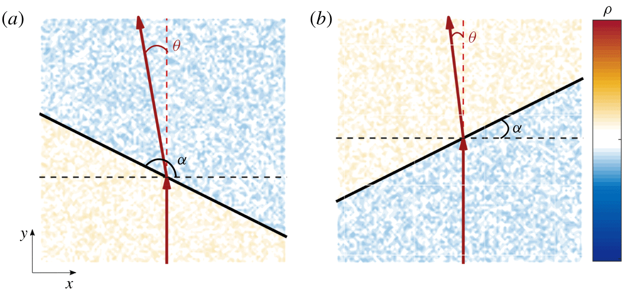A negative streamwise density gradient event, $\unicode[STIX]{x2202}\unicode[STIX]{x1D70C}/\unicode[STIX]{x2202}x<0$, assuming local isotropy (step change in density and index of refraction), would lead to an upstream deflection of the beam, denoted with a negative value for $\unicode[STIX]{x1D703}$, for all non-zero values of the angle $\unicode[STIX]{x1D6FC}$ between the density front and the horizontal axis (figure 2). Similarly, a positive streamwise density gradient event, $\unicode[STIX]{x2202}\unicode[STIX]{x1D70C}/\unicode[STIX]{x2202}x>0$, would lead to a downstream beam deflection, denoted with a positive $\unicode[STIX]{x1D703}$. The deflection angle $\unicode[STIX]{x1D703}$ can be connected to the density gradient field by ((2.2) Saxton-Fox et al. Reference Saxton-Fox, McKeon and Gordeyev2019)

(2.2)

$$\begin{eqnarray}\unicode[STIX]{x1D703}(y_{f},t)-\unicode[STIX]{x1D703}(y_{i})\approx \frac{K_{GD}}{1+K_{GD}\unicode[STIX]{x1D70C}_{a}}\int _{y_{i}}^{y_{f}}\frac{\unicode[STIX]{x2202}\unicode[STIX]{x1D70C}}{\unicode[STIX]{x2202}x}(x_{MP},y,z_{MP},t)\,\text{d}y,\end{eqnarray}$$

where $\unicode[STIX]{x1D703}(y_{i})$ and $\unicode[STIX]{x1D703}(y_{f},t)$ are the initial and final angles of the incoming beam respectively, $\unicode[STIX]{x1D70C}_{a}$ the ambient density of the fluid and $x_{MP},z_{MP}$ the streamwise–spanwise coordinates of the beam location. With respect to the PIV coordinate system (figure 1c), $(x_{MP},y,z_{MP})=(-0.33\unicode[STIX]{x1D6FF},0,0)$ for the upstream MP beam and $(x_{MP},y,z_{MP})=(-0.08\unicode[STIX]{x1D6FF},0,0)$ for the downstream one. All the results presented in this work refer to the downstream beam, which was approximately aligned with the centre of the field of view of the PIV system (see next section), but the trends and conclusions discussed in the following sections were identical for both beams.

Figure 2.

For $\unicode[STIX]{x2202}\unicode[STIX]{x1D70C}/\unicode[STIX]{x2202}x<0$ the beam experiences an upstream deflection regardless of the angle $\unicode[STIX]{x1D6FC}$, between the density front and the horizontal. Upstream leaning density front, $\unicode[STIX]{x2202}\unicode[STIX]{x1D70C}/\unicode[STIX]{x2202}y<0$, $\unicode[STIX]{x1D6FC}<\unicode[STIX]{x03C0}/2$ (a), downstream leaning density front, $\unicode[STIX]{x2202}\unicode[STIX]{x1D70C}/\unicode[STIX]{x2202}y>0$, $\unicode[STIX]{x1D6FC}>\unicode[STIX]{x03C0}/2$ (b). Warm and cool colours indicate higher and lower values for the density, respectively.

2.2 Velocity measurements

For the PIV measurements, Dioctyl – di(2-ethylhexyl) – sebacate liquid was used for the seeding, atomised with a LaVision Aerosol Generator into droplets with a nominal diameter $d_{p}=0.25~\unicode[STIX]{x03BC}\text{m}$, illuminated with a 527 nm single-head YLF Photonics laser (DM20-527) running in double pulse mode, with a pulse separation $dt=0.38~\unicode[STIX]{x03BC}\text{s}$. The 5 mm diameter laser beam was guided to the measurement location with the use of three mirrors each at a 45^° angle and was expanded into a streamwise–wall-normal sheet ∼2 mm thick, using a Powell lens.

Images were recorded using a Phantom Miro 320S high-speed camera with a 1920 × 1080 pixels CMOS sensor (10 μm) pixel size, fitted with a Tamron $f/3.5$ SP AF Macro lens with a focal length of 180 mm at an aperture stop of $f/8$. The system was synchronised using a LaVision high-speed controller. The camera captured a field of view approximately 0.035 m × 0.055 m ($0.99\unicode[STIX]{x1D6FF}\times 1.5\unicode[STIX]{x1D6FF}$), in $x$ and $y$ respectively, at 600 Hz ($1.8U_{\infty }/\unicode[STIX]{x1D6FF}$), with a resulting digital resolution of 29 pix mm^-1. We acquired $N_{tot}=19\,287$ images using DaVis 8.3.1 (in 9 independent time-resolved sets of 2143 images each), which we subsequently processed using the same software applying an iterative correlation with a final interrogation window of 32 × 32 pixels with an overlap factor of 50 %. The nominal flow conditions at the measurement location were: $U_{\infty }=12~\text{m}~\text{s}^{-1}$, $\unicode[STIX]{x1D6FF}=\unicode[STIX]{x1D6FF}_{99}=36~\text{mm}$, $Re_{\unicode[STIX]{x1D70F}}=1070$ (table 1). The friction velocity was computed using the Clauser chart method (Clauser Reference Clauser1954). For the computation of the momentum thickness, Spalding’s law of the wall (Spalding Reference Spalding1961) was employed for the region from the wall ( $y^{+}=0$) up to the first independent velocity point (i.e. the first point not influenced by the wall in the correlation process).

Figure 3.

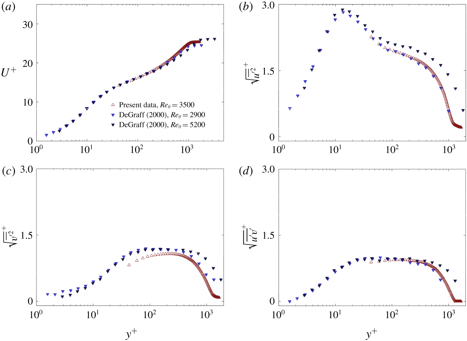
(a) Inner-normalised streamwise mean velocity. Inner-normalised r.m.s. values of streamwise (b), wall-normal velocity intensities (c) and Reynolds shear stress (d). Present data are compared with results from De Graaff & Eaton (Reference De Graaff and Eaton2000) at similar Reynolds numbers.

Table 1.

Nominal flow conditions.

The mean flow and turbulence statistics show overall good agreement with laser Doppler anemometry measurements of similar Reynolds numbers from De Graaff & Eaton (Reference De Graaff and Eaton2000), with the exception of the root-mean-squared (r.m.s.) values of the wall-normal velocity intensities, which are slightly under-resolved, especially close to the wall (figure 3).

2.3 Large magnitude MP deflections

The simultaneous PIV and MP measurements allow for the use of the MP signal as a condition on which the velocity fields can be averaged. Any scalar quantity $q$ can be conditionally averaged on large positive (downstream) or negative (upstream) MP angle fluctuations, $\unicode[STIX]{x1D703}(t)$ (2.3):

(2.3)

$$\begin{eqnarray}q|_{\unicode[STIX]{x1D703}}=\langle q\rangle |_{|\unicode[STIX]{x1D703}|>w\unicode[STIX]{x1D70E}_{\unicode[STIX]{x1D703}}},\end{eqnarray}$$

where $\unicode[STIX]{x1D70E}_{\unicode[STIX]{x1D703}}$ is the standard deviation of the fluctuating MP signal and $w$ is a threshold value, here chosen as $w=0.5$.

Figure 4.

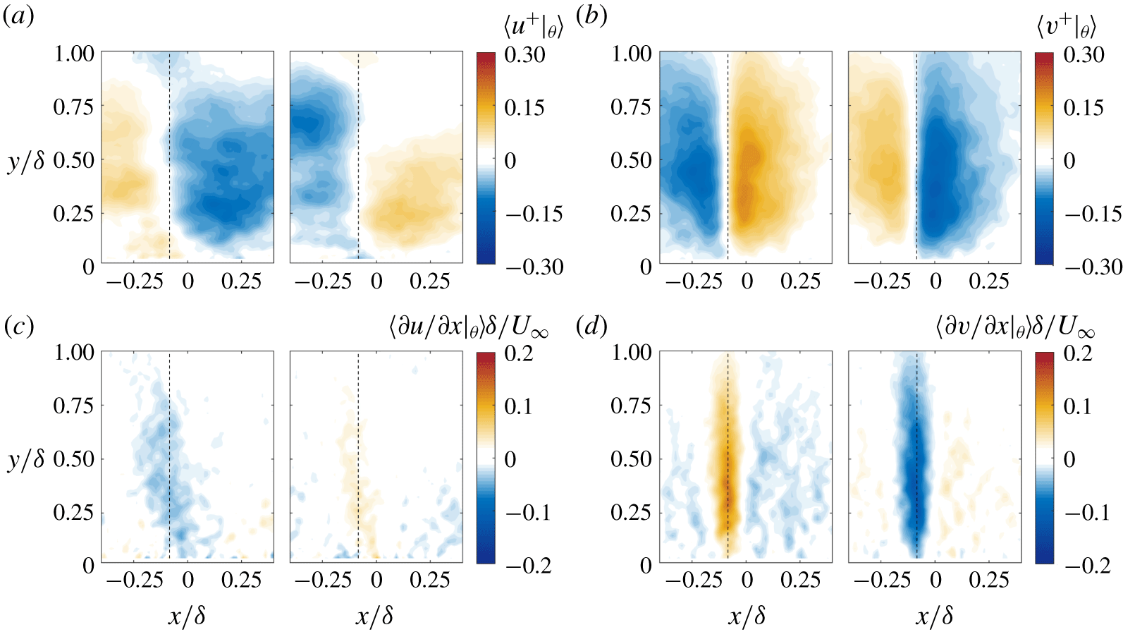
Contour plots of inner-normalised velocity fluctuations and their outer-normalised streamwise gradients, conditionally averaged on the MP deflection angle (negative deflection on the left and positive on the right for all panels). Black dashed lines indicate the MP location. Streamwise velocity fluctuations (a), and the corresponding streamwise gradient (c). Wall-normal velocity fluctuations (b), and the corresponding streamwise gradient (d).

In what follows, quantities with the subscript $\unicode[STIX]{x1D703}$ will denote averaging on a large MP deflection, the sign of which will be explicitly stated. With this threshold, approximately 60 % of the total PIV images acquired, $N_{tot}$, were associated with a large MP deflection, almost equally divided between negative and positive deflections (see table 2). Different values of $w$ have been tested and although the exact quantitative results varied, the main trends discussed herein were unaltered.

Table 2.

Percentage of frames and parameters for the Gaussian function $s_{G1}$, for both negative and positive large MP deflections.

In line with the observations from Saxton-Fox et al. (Reference Saxton-Fox, McKeon and Gordeyev2019), both fluctuating velocity fields, when conditioned on large beam deflections, show a change in sign across the MP measurement location that extends across the full boundary layer height (figures 4a and 4b). The sign of the MP deflection (and therefore of the streamwise scalar gradient) matches that of the streamwise velocity gradient (figure 4c), supporting the strong correlation of the two fields when $Pr$ number is close to unity, while the gradient of the wall-normal velocity is of the opposite sign and is shown to be stronger and more robust across $\unicode[STIX]{x1D6FF}$ (figure 4d). It is also interesting to note that, while the vertical velocity gradient is homogeneous across $y$, the streamwise velocity gradient shows a moderate upstream inclination angle, which will be further explored in the following section.

3 Results

The wall-normal coherence of the conditionally averaged fields (${>}\unicode[STIX]{x1D6FF}$) is much larger than the one observed in the instantaneous realisations, suggesting that it is a result of multiple smaller-scale structures, situated at different wall-normal locations across $\unicode[STIX]{x1D6FF}$ (Saxton-Fox et al. Reference Saxton-Fox, McKeon and Gordeyev2019). The goal of the present work is to identify such structures and explore their geometry for both the streamwise and wall-normal velocities. Since $\unicode[STIX]{x2202}v/\unicode[STIX]{x2202}x$ is shown to be the most robust and relatively homogeneous across $y$ in the conditionally averaged fields (figure 4d), we use its wall-normal average, $s_{1}(x)$, as a second condition upon which the velocity fields associated with large beam deflections will be further classified (figures 5a–5b, equation (3.1)),

(3.1)

$$\begin{eqnarray}s_{1}(x)=\left\langle \left.\!\frac{\unicode[STIX]{x2202}v}{\unicode[STIX]{x2202}x}\right|_{\unicode[STIX]{x1D703}}\right\rangle _{y}.\end{eqnarray}$$

Specifically, we assume that each instantaneous $\unicode[STIX]{x2202}v/\unicode[STIX]{x2202}x$ field associated with a large beam deflection, $s_{2i}$, will contain, at some $y$ location, a structure with similar streamwise signature as $s_{1}(x)$ (3.2),

(3.2)

$$\begin{eqnarray}s_{2i}=\frac{\unicode[STIX]{x2202}v}{\unicode[STIX]{x2202}x}(x,y),\end{eqnarray}$$

for $i=1,\ldots ,N|_{\unicode[STIX]{x1D703}}$, where $N|_{\unicode[STIX]{x1D703}}$ is the number of velocity fields associated with a large beam deflection. We then proceed to identify the wall-normal location, $y_{c}$, for which the correlation coefficient, $\unicode[STIX]{x1D70C}_{s_{1},s_{2i}}$ is maximum (see figure 5c, equation (3.3)),

(3.3)

$$\begin{eqnarray}\unicode[STIX]{x1D70C}_{s_{1},s_{2i}}(y)=\frac{\text{cov}(s_{1},s_{2i})}{\unicode[STIX]{x1D70E}_{s_{1}}\unicode[STIX]{x1D70E}_{s_{2i}}},\end{eqnarray}$$

with $y_{c}=\text{argmax}\unicode[STIX]{x1D70C}_{s_{1},s_{2i}}$. When averaged across all snapshots, $\unicode[STIX]{x1D70C}_{s_{1},s_{2}}=\langle \unicode[STIX]{x1D70C}_{s_{1},s_{2i}}\rangle$, the correlation coefficient reaches maximum values of 0.35 at $y_{c}$ (see figure 5f).

The shape of $s_{1}(x)$ can be approximated with a Gaussian function, $s_{G1}$ ((3.4), solid and dashed lines in figures 5a and 5b, respectively),

(3.4)

$$\begin{eqnarray}s_{G1}=\pm \unicode[STIX]{x1D6FC}\text{e}^{-(x-\unicode[STIX]{x1D6FD})^{2}/c^{2}},\end{eqnarray}$$

where a positive (negative) sign is for a negative (positive) MP deflection (figures 5d–5e). Apart from some minimal under- and over-shoot downstream of the peak, $s_{1}$ follows the Gaussian approximation exceptionally well. For the results that follow, $s_{G1}$ was used for the estimation of $\unicode[STIX]{x1D70C}_{s_{1},s_{2i}}$; the use of $s_{1}$ was also tested with negligible differences. The resulting parameters for the fitted Gaussian distributions indicate that the streamwise variation of $\unicode[STIX]{x2202}v/\unicode[STIX]{x2202}x$ is remarkably similar for both positive and negative MP deflections in terms of the centre ($\unicode[STIX]{x1D6FD}=x_{MP}$, where $x_{MP}$ is the MP location) and width (controlled by parameter $c$) of the peak (see table 2). The outer-normalised peak amplitude of the positive gradient (negative MP deflection) is shown to be slightly larger, a behaviour also observed for the streamwise velocity gradient (see figure 4c), and a point we will revisit later. The shape of $s_{1}$ indicates that, on average, the most prominent scale for $\unicode[STIX]{x2202}v/\unicode[STIX]{x2202}x$ is ${\sim}0.2\unicode[STIX]{x1D6FF}$ (figures 5a and 5b). The main focus here is to analyse velocity structures which are associated with the presence of such a scale in the streamwise gradient of the wall-normal velocity. However, the fact that $s_{1}$ can be well approximated by an analytical expression allows us to also assess the resulting $u$ and $v$ structural characteristics in the case of wider ($c^{\ast }=2c$) and narrower ($c^{\ast }=0.5c$) distributions for $\unicode[STIX]{x2202}v/\unicode[STIX]{x2202}x$ (see figure 5).

Figure 5.

(a,b) Wall-normal average of the contour plots in figure 4(d) for a negative and positive MP deflection, respectively. Solid lines denote the Gaussian approximation of the profile, $s_{G1}$, for increasing peak width, $c^{\ast }$, and symbols denote $s_{1}$. (c) Instantaneous profile of $\unicode[STIX]{x1D70C}_{s_{1},s_{2}}$. Red dotted line indicates the location, $y_{c}$, where $\unicode[STIX]{x1D70C}_{s_{1},s_{2}}$ is maximum. (d,e) Probability density function of $y_{c}$ for negative and positive MP deflections, respectively. Coloured bars denote $s_{1}$ and solid lines its Gaussian approximation, $s_{G1}$, for increasing peak width, $c^{\ast }$. (f) Average profile of the correlation coefficient $\unicode[STIX]{x1D70C}_{s_{1},s_{2}}=\langle \unicode[STIX]{x1D70C}_{s_{1},s_{2i}}\rangle$ for different values of $c^{\ast }$.

The probability density function of $y_{c}$ for both negative and positive MP deflections suggests that, in most cases, structures more strongly correlated with the average behaviour described by $s_{1}$, are found at locations close to the middle of the boundary layer, $y\approx 0.4\unicode[STIX]{x1D6FF}$ (figures 5d–5e). This trend becomes stronger for wider distributions of $s_{1}$, indicating that smaller structures in $x$ are more evenly distributed across $\unicode[STIX]{x1D6FF}$, but as their streamwise extent increases, they tend to cluster around the middle of the boundary layer. The local mean velocity at that wall-normal location ( $y=0.4\unicode[STIX]{x1D6FF}$) is ${\sim}0.83U_{\infty }$, matching the prevalent convection velocity of optical disturbances found by Gordeyev et al. (Reference Gordeyev, Smith, Cress and Jumper2014). The effect of scale is also reflected on the average correlation coefficient, $\langle \unicode[STIX]{x1D70C}_{s_{1},s_{2i}}\rangle$, which increases in amplitude and becomes narrower in $y$ for narrower distributions of $s_{1}$ in $x$ (figure 5f). The former indicates that, instantaneously, a narrower distribution of $s_{1}$ in $x$ is more prevalent, hence the higher amplitude, while the latter shows that a decrease in the streamwise extent of $\unicode[STIX]{x2202}v/\unicode[STIX]{x2202}x$ is linked to a decrease in the wall-normal one as well.

The location of maximum correlation $y_{c}$ can then be used as a second condition upon which to average the velocity fields, a procedure denoted in what follows with the subscript $y_{c}$. In particular, instantaneous velocity fields that are associated with large MP deflections using the first condition outlined above, are classified further based on the location of $y_{c}$; for convergence purposes, 5 regions are considered: $y_{c}\in [0,0.2\unicode[STIX]{x1D6FF})$, $y_{c}\in [0.2\unicode[STIX]{x1D6FF},0.4\unicode[STIX]{x1D6FF})$, $y_{c}\in [0.4\unicode[STIX]{x1D6FF},0.6\unicode[STIX]{x1D6FF})$, $y_{c}\in [0.6\unicode[STIX]{x1D6FF},0.8\unicode[STIX]{x1D6FF})$ and $y_{c}\in [0.8\unicode[STIX]{x1D6FF},1.0\unicode[STIX]{x1D6FF})$, with $y_{cm}$ denoting the mid-point of each region. Using the snapshots classified to each of these regions, the conditional velocity fields $\langle u^{+}|_{\unicode[STIX]{x1D703},y_{c}}\rangle$ and $\langle v^{+}|_{\unicode[STIX]{x1D703},y_{c}}\rangle$ are computed, using a moving frame of reference parallel to the Cartesian one but with the origin at $y_{c}$, independent of where $y_{c}$ is located with respect to the wall. Thus, for each region chosen, $u$ and $v$ profiles are collected along $y-y_{c}$ and are all centred at $y_{c}$; since their origin is the same, averaging across the snapshots classified to each region will highlight the velocity variation in the vicinity of $y_{c}$ with the wall-normal extent being largely independent of the size of the regions chosen (figure 6). This is a result of both the choice of origin when averaging, but also the fact that the size of the structures is shown to be almost constant across $y$. If a single region was chosen containing all snapshots, the resulting velocity fields would have extents very similar to those in figures 6 and 7, but the variation in intensity between positive and negative velocity structures as $y_{c}$ moves away from the wall would not be captured. If on the other hand, more regions were considered, resulting in a finer resolution, the averaged fields would still exhibit a similar wall-normal extent but convergence issues would arise due to the decreasing number of snapshots included in each region.

Figure 6.

Contour plots of inner-normalised velocity fluctuations, conditionally averaged on both a negative MP deflection angle ($\unicode[STIX]{x1D703}<-0.5\unicode[STIX]{x1D70E}_{\unicode[STIX]{x1D703}}$) and on $y_{c}$. The five panels are, from left to right: $y_{c}\in [0,0.2\unicode[STIX]{x1D6FF})$, $y_{c}\in [0.2\unicode[STIX]{x1D6FF},0.4\unicode[STIX]{x1D6FF})$, $y_{c}\in [0.4\unicode[STIX]{x1D6FF},0.6\unicode[STIX]{x1D6FF})$, $y_{c}\in [0.6\unicode[STIX]{x1D6FF},0.8\unicode[STIX]{x1D6FF})$ and $y_{c}\in [0.8\unicode[STIX]{x1D6FF},1.0\unicode[STIX]{x1D6FF})$. Vertical dashed lines denote the MP location. (a) Streamwise velocity fluctuations. (b) Wall-normal velocity. (c) Streamlines using the full velocity field and subtracting $U_{c}=\langle U(x,y_{cm})\rangle _{x}$, indicating that $\unicode[STIX]{x2202}\unicode[STIX]{x1D70C}/\unicode[STIX]{x2202}x<0$ events are aligned with diverging separatrices, going through saddle points, in line with observations from Antonia & Fulachier (Reference Antonia and Fulachier1989) on coolings.

Figure 7.

Contour plots of inner-normalised velocity fluctuations, conditionally averaged on both a positive MP deflection angle ($\unicode[STIX]{x1D703}>0.5\unicode[STIX]{x1D70E}_{\unicode[STIX]{x1D703}}$) and on $y_{c}$. The Gaussian approximation $s_{G1}$ was used for the computation of $\unicode[STIX]{x1D70C}_{s_{1},s_{2}}$, with $c^{\ast }=c$. The five panels are, from left to right: $y_{c}\in [0,0.2\unicode[STIX]{x1D6FF})$, $y_{c}\in [0.2\unicode[STIX]{x1D6FF},0.4\unicode[STIX]{x1D6FF})$, $y_{c}\in [0.4\unicode[STIX]{x1D6FF},0.6\unicode[STIX]{x1D6FF})$, $y_{c}\in [0.6\unicode[STIX]{x1D6FF},0.8\unicode[STIX]{x1D6FF})$ and $y_{c}\in [0.8\unicode[STIX]{x1D6FF},1.0\unicode[STIX]{x1D6FF})$. Vertical dashed lines denote the MP location. (a) Streamwise velocity fluctuations. (b) Wall-normal velocity. (c) Streamlines using the full velocity field and subtracting $U_{c}=\langle U(x,y_{cm})\rangle _{x}$, indicating that $\unicode[STIX]{x2202}\unicode[STIX]{x1D70C}/\unicode[STIX]{x2202}x>0$ events are aligned with unstable foci, in line with observations from Antonia & Fulachier (Reference Antonia and Fulachier1989) on heatings.

Results indicate that the wall-normal velocity structures which instantaneously exhibit the strongest correlation with the average behaviour (in terms of $\unicode[STIX]{x2202}v/\unicode[STIX]{x2202}x$), are localised in $y$. The emerging picture is that of a pair of elliptical $v$ structures of opposing signs (depending on the underlying density gradient) on either side of the MP location $x_{MP}$, (figures 6b–7b). Their intensity is shown to decrease as they approach the free stream, while their size appears to only vary slightly with wall-normal location, particularly in the case of the negative MP deflection (figure 6b). Regarding the streamwise velocity field, the conditional structures leading to the average behaviour (figure 4a) are shown to exhibit the expected sign change at the MP location, consistent with the sign of the underlying density gradient (figures 6a–7a). Interestingly, this happens across an upstream leaning interface where $\langle u^{+}|_{\unicode[STIX]{x1D703},y_{c}}\rangle =0$, indicating that the most prominent geometry associated with a negative MP deflection is that of an upstream leaning velocity front. The average behaviour, across all $y$ locations, of the streamwise velocity gradient, hinted at that (see figure 4c), although the effect was significantly weaker.

For large negative MP deflections, this upstream slope is fairly narrow, centred around the MP location (solid vertical line in figure 6a), and it is seen to be imposed on a larger-scale, downstream leaning $\langle u^{+}|_{\unicode[STIX]{x1D703},y_{c}}\rangle =0$ contour, creating a sawtooth profile. This highlights the multiscale nature of this phenomenon and is in line with the modelling work of Saxton-Fox et al. (Reference Saxton-Fox, McKeon and Gordeyev2019), where the main features of the flow could be reproduced assuming a superposition of different velocity scales. For large positive MP deflections, the larger-scale structure is absent and the upstream leaning $\langle u^{+}|_{\unicode[STIX]{x1D703},y_{c}}\rangle =0$ contour dominates the conditional structure across $x$ (figure 6b). Another trend observed, irrespective of the sign of the beam deflection, is a monotonic decrease of the magnitude of positive $u$ fluctuations as $y$ increases, while low-speed regions become more prominent. For a negative MP deflection, this is also combined with a marked decrease of the negative $v$ fluctuations with increasing distance from the wall, such that close to the free-stream ejection events ($u<0$, $v>0$) are dominant. This is in line with observations in Saxton-Fox et al. (Reference Saxton-Fox, McKeon and Gordeyev2019) where the height of the small-scale vertical velocity structures was found to be dependent on the phase of the large-scale streamwise velocity motion.

The addition of the mean flow field $\overline{U}$ and the subtraction of a constant convection velocity allows the analysis of the flow topology associated with these conditional velocity fluctuations at each region of $y_{c}$. For a convection velocity $U_{c}$, equal to the mean velocity at the mid-point of each region $y_{cm}$, the resulting streamlines highlight the presence of a saddle point for the case of a negative MP deflection and a focus point in the case of a positive deflection (figures 6c–7c), a behaviour consistent throughout the boundary layer. The same critical point behaviour was observed by Antonia & Fulachier (Reference Antonia and Fulachier1989) who used concurrent temperature and velocity measurements from cold-wire and hot-wire anemometry respectively, and analysed the flow topology conditioned on the presence of strong negative (coolings) and positive (heatings) temperature gradients in time. Taking into account the relationship between temperature and density in an ideal gas and the analogy between density gradients and the measured MP angle (2.2), we can conclude that heatings in time would be consistent with strong positive MP deflections (positive streamwise density gradients), while coolings could be identified with negative MP deflections (negative streamwise density gradients). This association between MP deflections and temperature fronts detected from cold-wire rakes is also supported by the work of Subramanian et al. (Reference Subramanian, Rajagopalan, Antonia and Chambers1982). These authors compared different event detection techniques and concluded that both warm and cool fronts are spatially coherent and potentially demarcate the boundaries between different quadrant events: the former that of a sweep followed (in time) by an ejection (in agreement with the conditional $u$ and $v$ fields in the present study for a positive MP deflection, figure 7) and the latter that of an ejection followed by a sweep (observed in the velocity fields depicted in figure 6). Conditional averages of velocity fluctuations around a cool front by Antonia et al. (Reference Antonia, Rajagopalan, Subramanian and Chambers1982) also highlighted the prevalence of ejection events close to the free stream, as was also observed in the present data for a negative MP deflection.

Although there are several differences between the two measurement techniques, the strong similarities in the resulting conditional velocity jumps and flow topologies support the assumption that the underlying flow structures giving rise to strong aero-optic distortions of a certain orientation, and to temperature gradients of a certain sign are closely connected.

In the following two sections, an effort is made to analyse in more detail the geometrical characteristics of $\langle u^{+}|_{\unicode[STIX]{x1D703},y_{c}}\rangle$ and $\langle v^{+}|_{\unicode[STIX]{x1D703},y_{c}}\rangle$ (figures 6–7) as well as assessing their dependence on different streamwise scales for $s_{1}$ (figures 5a–5b).

3.1 Vertical velocity

As mentioned earlier, when conditioned both on a large MP deflection and $y_{c}$, the vertical velocity fluctuations are localised in $y$, their extent being elliptical in shape, with two structures of opposing sign on either side of the MP location (see figures 6b–7b). In order to quantify the extent of the structures for the different wall-normal locations, an elliptical fit is used at 40 % of the absolute peak magnitude, where $\unicode[STIX]{x1D6EC}_{x}$ and $\unicode[STIX]{x1D6EC}_{y}$ denote the streamwise and wall-normal extent of fit, respectively, and $X_{e}$ and $Y_{e}$ are the coordinates of the centre (figure 8). The absolute peak magnitudes, $\max |\langle v^{+}|_{\unicode[STIX]{x1D703},y_{c}}\rangle |$, indicate that positive and negative fluctuations close to the wall have comparable strength, irrespective of the MP deflection sign (figure 8b). However, a moderate decrease in peak magnitude with $y$ for negative fluctuations is observed, such that at the free-stream positive fluctuations (associated with ejecting motions) are prominent. It should be noted here that, even when narrower ($c^{\ast }=0.5c$) and wider ($c^{\ast }=2c$) streamwise distributions are considered for the average gradient of the wall-normal velocity, $s_{G1}$ (see (3.4)), this behaviour for the peak magnitudes of the resulting wall-normal velocity fluctuations remains remarkably unaltered (lighter coloured solid lines in figure 8b).

Figure 8.

Geometrical characteristics for $\langle v^{+}|_{\unicode[STIX]{x1D703},y_{c}}\rangle$ (figures 6–7). (a) Elliptical fits for the conditionally averaged wall-normal velocity fluctuation contours from figures 6 and 7 at 40 % of the peak magnitude and for all $y_{c}$ locations: $y_{c}\in [0,0.2\unicode[STIX]{x1D6FF})$, $y_{c}\in [0.2\unicode[STIX]{x1D6FF},0.4\unicode[STIX]{x1D6FF})$,$y_{c}\in [0.4\unicode[STIX]{x1D6FF},0.6\unicode[STIX]{x1D6FF})$, $y_{c}\in [0.6\unicode[STIX]{x1D6FF},0.8\unicode[STIX]{x1D6FF})$ and $y_{c}\in [0.8\unicode[STIX]{x1D6FF},1.0\unicode[STIX]{x1D6FF})$. (b) Variation of the peak magnitude, $\max |\langle v^{+}|_{\unicode[STIX]{x1D703},y_{c}}\rangle |$ with $y_{cm}$. Colours from darker to lighter for increasing $c^{\ast }=0.5c,1c,2c$. Solid lines in (a) and (b) denote a negative MP deflection, and dashed lines a positive one. Negative velocity fluctuations are denoted by blue while positive ones with red. (c) Here, $\unicode[STIX]{x1D6EC}_{x}$ and $\unicode[STIX]{x1D6EC}_{y}$ denote the streamwise and wall-normal extent of the elliptical contours, respectively, while $X_{e}$ and $Y_{e}$ are the coordinates of their centres.

With respect to the streamwise extent $\unicode[STIX]{x1D6EC}_{x}$ of the elliptical structures, the first thing to note is that results for both positive and negative $v$ fluctuations are similar but more striking is the correspondence between the case of positive and negative MP deflections (dashed and solid lines respectively in figures 9a–9b), indicating an almost anti-symmetrical $\langle v^{+}|_{\unicode[STIX]{x1D703},y_{c}}\rangle$ field around the MP location for either case. The main difference in behaviour is observed for the wall-normal locations closer to the free stream, where downwards moving motions become narrower in $x$, especially for the negative MP deflection, while the positive fluctuations remain almost constant up to the edge of the boundary layer. For both positive and negative fluctuations, the average streamwise extent is ${\sim}0.1\unicode[STIX]{x1D6FF}$ for $c^{\ast }=c$. Allowing the average signature of $\unicode[STIX]{x2202}v/\unicode[STIX]{x2202}x$ to vary in streamwise width ($c^{\ast }=0.5c,1c,2c$), the resulting $v$ structures that are identified show a similar variation in streamwise extent, although not in a linear sense: a doubling in $c$ for $\unicode[STIX]{x2202}v/\unicode[STIX]{x2202}x$ leads to approximately a doubling in $\unicode[STIX]{x1D6EC}_{x}$ for $v$. However, for $c^{\ast }=0.5c$ the resulting $v$ structures exhibit only a minimal decrease in $\unicode[STIX]{x1D6EC}_{x}$, indicating perhaps the existence of a minimum.

Figure 9.

Variation with $y_{cm}$ for the streamwise and wall-normal extent, $\unicode[STIX]{x1D6EC}_{x}$ and $\unicode[STIX]{x1D6EC}_{y}$ and the centroid coordinates, $X_{e}$ and $Y_{e}$, of the elliptical fits of the wall-normal velocity fluctuations (defined in figure 8c). In all panels, transition from darker to lighter colours (highlighted with arrows) indicates an increasing peak width ($c^{\ast }=0.5c,1c,2c$) for $s_{G1}$ (3.4). (a,d) $\unicode[STIX]{x1D6EC}_{x}$ and $\unicode[STIX]{x1D6EC}_{y}$ for $\langle v^{+}|_{\unicode[STIX]{x1D703},y_{c}}\rangle >0$. (b,e) $\unicode[STIX]{x1D6EC}_{x}$ and $\unicode[STIX]{x1D6EC}_{y}$ for $\langle v^{+}|_{\unicode[STIX]{x1D703},y_{c}}\rangle <0$. Solid lines for a negative MP deflection and dashed for a positive one. (c,f) $X_{e}$ and $Y_{e}$ for a negative MP deflection.

The wall-normal extent $\unicode[STIX]{x1D6EC}_{y}$, shows a very similar behaviour to $\unicode[STIX]{x1D6EC}_{x}$ for the negative $v$ fluctuations, varying marginally with $y$, except at the edge of the boundary layer where a sharp decrease in extent is observed for the negative MP deflection (solid lines in figure 9e). The conditionally averaged fields do not allow for further insight into this particular trend although, generally, larger discrepancies are expected close to the free stream due to the decrease in magnitude for the fluctuations. Varying the streamwise width of the average $\unicode[STIX]{x2202}v/\unicode[STIX]{x2202}x$ signature $s_{G1}$, has a minor effect on the wall-normal extent of the identified localised structures, that becomes more pronounced far away from the wall for the negative $v$ fluctuations. The wall-normal extent variation for the positive $v$ fluctuations shows again a very close correspondence for both positive and negative MP deflections and a moderate increase with $y$. A decrease of $c^{\ast }$ leads to a negligible decrease in $\unicode[STIX]{x1D6EC}_{y}$.

In terms of the centre of the elliptical fit ($X_{e}$, $Y_{e}$), results indicate that it remains effectively constant for all wall-normal locations (figures 9c and 9f for a negative MP deflection), in line with the tall vertical structures for both $\langle v\rangle |_{\unicode[STIX]{x1D703}}$ and $\langle \unicode[STIX]{x2202}v/\unicode[STIX]{x2202}x\rangle |_{\unicode[STIX]{x1D703}}$ which are almost homogeneous across $y$ (figures 4b and 4d). This trend was also observed for a positive MP deflection (not shown here). Increasing the streamwise width of $s_{G1}$ leads to an increase in the streamwise extent of the resulting conditional $v$ structures (figures 9a–9b), which is also reflected as an increase in the distance between the centres of the two elliptical structures in either side of the MP (increasing $c^{\ast }$ in figure 9c).

Overall these observations are in line with the conceptual model introduced by Saxton-Fox et al. (Reference Saxton-Fox, McKeon and Gordeyev2019) where the tall, conditionally averaged $v$ structures (figure 4b), are a result of a superposition of smaller-scale $v$ events, of similar size, sitting at different heights from the wall (figure 10).

Figure 10.

Contours of inner-normalised vertical velocity fluctuations, $\langle v^{+}|_{\unicode[STIX]{x1D703},y_{c}}\rangle$, at 30 % of their peak magnitude, conditionally averaged on both a large MP deflection and on $y_{c}$ (from figures 6b and 7b), supporting the conceptual schematic proposed by Saxton-Fox et al. (Reference Saxton-Fox, McKeon and Gordeyev2019); $\unicode[STIX]{x1D703}<-0.5\unicode[STIX]{x1D70E}_{\unicode[STIX]{x1D703}}$ (a), $\unicode[STIX]{x1D703}>0.5\unicode[STIX]{x1D70E}_{\unicode[STIX]{x1D703}}$ (b).

3.2 Streamwise velocity

The emerging picture from the conditionally averaged $u$ structures, $\langle u^{+}|_{\unicode[STIX]{x1D703},y_{c}}\rangle$, is that of a multiscale phenomenon, especially for the case of a negative MP deflection (figure 6a). In particular, the resulting fields indicate that at the MP location $\langle u^{+}|_{\unicode[STIX]{x1D703},y_{c}}\rangle$ experiences a change in sign in the streamwise direction, as dictated by the underlying scalar gradient ($\unicode[STIX]{x2202}u/\unicode[STIX]{x2202}x|_{(x_{MP},y_{c})}<0$, for a negative MP deflection). However, that happens across an upstream leaning contour ($\langle u^{+}|_{\unicode[STIX]{x1D703},y_{c}}\rangle =0$), thus implying that the wall-normal gradient has the same sign ($\unicode[STIX]{x2202}u/\unicode[STIX]{x2202}y|_{(x_{MP},y_{c})}<0$, for a negative MP deflection). Away from the MP location, there is a clear signature of a downstream leaning larger-scale structure where $\unicode[STIX]{x2202}u/\unicode[STIX]{x2202}y$ and $\unicode[STIX]{x2202}u/\unicode[STIX]{x2202}x$ have opposing signs ($\unicode[STIX]{x2202}u/\unicode[STIX]{x2202}x<0$, still consistent with the scalar streamwise gradient). In an effort to distinguish these two effects, a third condition is introduced for the streamwise velocity fields, identifying whether at the point ($x_{MP},y_{c}$) the streamwise and wall-normal gradients of $u$ have the same (upstream leaning front, $\unicode[STIX]{x1D719}_{u}$) or opposing (downstream leaning front, $\unicode[STIX]{x1D719}_{d}$) signs (3.5),

(3.5)

$$\begin{eqnarray}\left.\begin{array}{@{}c@{}}\displaystyle c_{\unicode[STIX]{x1D719}}=\left.\frac{\unicode[STIX]{x2202}u}{\unicode[STIX]{x2202}x}\frac{\unicode[STIX]{x2202}u}{\unicode[STIX]{x2202}y}\right|_{x_{MP},y_{c}}\!,\\ u|_{\unicode[STIX]{x1D719}_{d}}=\langle u\rangle |_{c_{\unicode[STIX]{x1D719}}<0},\\ u|_{\unicode[STIX]{x1D719}_{u}}=\langle u\rangle |_{c_{\unicode[STIX]{x1D719}}>0}.\end{array}\right\}\end{eqnarray}$$

Additionally, since this condition highlights a scale separation between larger, downstream inclining ($\unicode[STIX]{x1D719}_{d}$) and smaller, upstream leaning ($\unicode[STIX]{x1D719}_{u}$) contours of $\langle u^{+}|_{\unicode[STIX]{x1D703},y_{c},\unicode[STIX]{x1D719}}\rangle =0$, a variation in $c^{\ast }$ can potentially further amplify this difference. As was mentioned earlier, the streamwise width of $s_{G1}$ (determined by $c^{\ast }$) allows for the identification of conditional $v$ structures with different streamwise lengths; therefore it can also be exploited to increase the scale separation already present in the $u$ velocity fields. Indeed, larger $c^{\ast }$ values than average ($c^{\ast }=2c$) lead to a prominence of the downstream leaning structures, while the smaller scales become more pronounced for narrower $s_{G1}$ profiles ($c^{\ast }=0.5c$). As such, to quantify the slopes corresponding to these events at different wall-normal locations, a value of $c^{\ast }=0.5c$ will be used for the fields conditioned on $\unicode[STIX]{x1D719}_{u}$ (upstream leaning structures), while $c^{\ast }=2c$ will be used for the opposite condition, $\unicode[STIX]{x1D719}_{d}$ (downstream leaning structures). Results indicate that, for a negative MP deflection, the downstream leaning structures are much more pronounced and have a larger extent in $x$ ($\unicode[STIX]{x1D719}_{d}$, figure 11a, left). For a positive MP deflection the resulting downstream leaning contour ($\langle u^{+}|_{\unicode[STIX]{x1D703},y_{c},\unicode[STIX]{x1D719}}\rangle =0$), although shorter, is also approximately linear. Remarkably, the linear fits of these contours indicate an almost constant slope across $y$, approximately equal for both positive and negative MP deflections (figures 12a, 12c), with an average angle $\unicode[STIX]{x1D719}_{d}\sim 20^{\circ }$ (figure 12e). This breaks down at the edge of the boundary layer, where negative $u$ fluctuations become prominent and the $\langle u^{+}|_{\unicode[STIX]{x1D703},y_{c},\unicode[STIX]{x1D719}}\rangle =0$ contour harder to identify. For both a negative and positive MP deflection, throughout the majority of the boundary layer, the percentage of such events with respect to the total is below 50 % and as low as 35 % near the wall (figure 12d). This indicates that, structures which instantaneously exhibit a strong streamwise gradient in the wall-normal velocity, of either sign (described by $s_{G1}$), will most often exhibit a gradient in the streamwise velocity across an upstream leaning interface for the majority of the boundary layer.

Figure 11.

Contour plots of inner-normalised streamwise velocity fluctuations, conditionally averaged on the MP deflection angle, the wall-normal location $y_{c}$ ( $y_{c}\in [0.4\unicode[STIX]{x1D6FF},0.6\unicode[STIX]{x1D6FF})$) and the sign of $c_{\unicode[STIX]{x1D719}}=(\unicode[STIX]{x2202}u/\unicode[STIX]{x2202}x)(\unicode[STIX]{x2202}u/\unicode[STIX]{x2202}y)|_{x_{MP},y_{c}}$ (3.5). For both images: $\unicode[STIX]{x1D703}<-0.5\unicode[STIX]{x1D70E}_{\unicode[STIX]{x1D703}}$ (left), $\unicode[STIX]{x1D703}>0.5\unicode[STIX]{x1D70E}_{\unicode[STIX]{x1D703}}$ (right). (a) For a downstream leaning contour ($\unicode[STIX]{x1D719}_{d}$, solid purple lines), $c^{\ast }=2c$. (b) For an upstream leaning contour ($\unicode[STIX]{x1D719}_{u}$), $c^{\ast }=0.5c$ (solid cyan lines on the right).

Figure 12.

Characteristics for $\langle u^{+}|_{\unicode[STIX]{x1D703},y_{c},\unicode[STIX]{x1D719}}\rangle =0$ contours. Solid and dashed lines indicate a negative and positive MP deflection, respectively. Grey lines in (a–c) denote linear fits and dashed vertical lines the MP location. (a) Variation with wall-normal location for $\unicode[STIX]{x1D719}=\unicode[STIX]{x1D719}_{d}$ and $c^{\ast }=2c$. (b) Variation with wall-normal location for $\unicode[STIX]{x1D719}=\unicode[STIX]{x1D719}_{u}$ and $c^{\ast }=0.5c$. (c) The angles $\unicode[STIX]{x1D719}_{u}$ and $\unicode[STIX]{x1D719}_{d}$ of the linear fits in (a) and (b) are defined with respect to the horizontal. (d) Percentage of events where $c_{\unicode[STIX]{x1D719}}>0$ ($\unicode[STIX]{x1D719}=\unicode[STIX]{x1D719}_{u}$) and $c_{\unicode[STIX]{x1D719}}<0$ ($\unicode[STIX]{x1D719}=\unicode[STIX]{x1D719}_{d}$) with respect to the total number of events, per wall-normal location. Colours as in (a–c). A transition from darker to lighter colours indicates an increasing peak width ($c^{\ast }=0.5c,1c,2c$) for $s_{G1}$ (3.4). (e) Variation of the angles $\unicode[STIX]{x1D719}_{u}$ and $\unicode[STIX]{x1D719}_{d}$ as defined in (c), per wall-normal location.

For a positive beam deflection this trend remains constant up to the edge of the boundary layer and only varies with different values of $c^{\ast }$. Specifically, as the width of $\unicode[STIX]{x2202}v/\unicode[STIX]{x2202}x$ increases ($c^{\ast }=2c$), the more strongly correlated $u$ structures seem to exhibit a change in sign across upstream and downstream leaning contours in equal measure. When smaller structures are identified ($c^{\ast }=0.5c$), the disparity between upstream and downstream leaning contours increases, with the former being more than two thirds of the total, indicating that they are indeed the manifestation of a smaller-scale phenomenon (dashed lines in figure 12d).

For a negative MP deflection and only close to the free-stream boundary, both upstream and downstream leaning fronts become almost equally probable, which perhaps explains why the downstream leaning signature is pronounced in the conditional fields even without imposing the condition on the slope, $c_{\unicode[STIX]{x1D719}}$ (see (3.5)). An increase in the streamwise width of $\unicode[STIX]{x2202}v/\unicode[STIX]{x2202}x$ used to identify the localised structures has a similar effect as in the positive deflection case, albeit much less pronounced; increase in $c^{\ast }$ leads to an increase of downstream leaning contours – a manifestation of a larger-scale phenomenon (solid lines in figure 12d).

When $\unicode[STIX]{x2202}u/\unicode[STIX]{x2202}y$ and $\unicode[STIX]{x2202}u/\unicode[STIX]{x2202}x$ are of the same sign (upstream leaning interface), the resulting contour separating negative from positive streamwise fluctuations is approximately linear and more pronounced in the case of a positive MP deflection (figure 11b, right). For a negative MP deflection this change in sign happens across a much smaller extent and the contour deviates from the linear approximation on both ends very rapidly (figure 11b, left). The slope of the linear fits is shown again to be almost constant across $y$ and fairly similar for both a negative and a positive MP deflection, with an average angle $\unicode[STIX]{x1D719}_{u}\sim 145^{\circ }$. As was discussed above, the average behaviour of the streamwise gradient of $v$ for a large MP deflection is more strongly correlated with $u$ structures of opposite signs, where in most cases the sign change happens across interfaces of this orientation with respect to the horizontal.

The overall notion discussed here, that of a multiscale structure associated with the backs of the turbulent bulges (regions where the large-scale motion exhibits a negative streamwise velocity gradient), has been examined in earlier studies, for example in Falco (Reference Falco1977) in the form of ‘typical eddies’ superimposed on the backs of the large-scale bulges present in the outer layer. More recently, the conceptual model of Saxton-Fox et al. (Reference Saxton-Fox, McKeon and Gordeyev2019) analysed the small-scale behaviour of the wall-normal velocity with respect to the phase of the large-scale $u$ motions; here an attempt is made to also characterise the average behaviour of the small-scale $u$ events. In studies where the scalar was directly measured, a comparable behaviour was found for the scalar (see for example the temperature ramp model suggested by Gibson et al. (Reference Gibson, Friehe and McConnell1977)), analysed often within the context of temperature derivative skewness (Sreenivasan & Antonia Reference Sreenivasan and Antonia1977). However, as was mentioned earlier, although a correlation between the scalar and the streamwise velocity would be expected, the available measurements in this study do not allow for a direct analogy between the two fields.

Finally, it should be noted that, the discussion here has been focused on the velocity structures within the turbulent region of the flow, which are linked to large MP deflections. These are found to reside in different wall-normal locations across the boundary layer height and include structures associated with the geometry of the turbulent/non-turbulent interface. Although large scalar gradients are expected in this region, results do not indicate that their effect on the beam deflection would be more dominant than the influence of other gradient events within the fully turbulent region.

4 Time scales of large MP deflections

One of the advantages of the MP technique is that it provides high time resolution signals for the beam deflection (32 kHz in this work), allowing us to characterise the time scales of large positive and negative deflections.

Figure 13.

Temporal characteristics of large magnitude MP events. (a) Segment of time signal of the MP deflection $\unicode[STIX]{x1D703}$. Squares denote positive (gold) and negative (green) large-scale events. (b) Variation of the relative number of positive and negative MP deflection events with increasing threshold $w=|\unicode[STIX]{x1D703}|/\unicode[STIX]{x1D70E}_{\unicode[STIX]{x1D703}}$. (c) Variation of the average period, $\overline{T}_{\unicode[STIX]{x1D703}\unicode[STIX]{x1D703}}$ between two successive negative or positive events with $w$.

In what follows, the outer-normalised ($U_{\infty }/\unicode[STIX]{x1D6FF}$) temporal scales of large negative ($L_{\unicode[STIX]{x1D703}_{-}}$) and positive ($L_{\unicode[STIX]{x1D703}_{+}}$) MP deflections, as well as the period $T_{\unicode[STIX]{x1D703}\unicode[STIX]{x1D703}}$ between events, are analysed (see figure 13). For the latter, a subscript $\unicode[STIX]{x1D703}_{-}\unicode[STIX]{x1D703}_{+}$ defines the period between a negative event followed by positive one.

As was discussed in § 4, the number of PIV snapshots associated with positive and negative MP events for a threshold value $w=|\unicode[STIX]{x1D703}|/\unicode[STIX]{x1D70E}_{\unicode[STIX]{x1D703}}=0.5$ (see (2.3)) is almost equal, each representing 30 % of the total number of snapshots (table 2). In this section we will consider all large magnitude MP events, not only the ones associated with PIV snapshots. A series of points, consecutive in time, all satisfying the condition (2.2) will be considered a single event (green and gold squares in figure 13a). To remove spurious fluctuations, events including more than three consecutive points in time ($L_{\unicode[STIX]{x1D703}}>0.03\unicode[STIX]{x1D6FF}/U\infty$) satisfying the large magnitude condition, are considered.

Using this definition for large magnitude events and a threshold value $w=0.5$, positive and negative events are still shown to be equal in number. By increasing this threshold, the relative number of identified negative deflections becomes increasingly larger compared to the positive ones. For a threshold $w=3$ the identified negative deflections are more than twice the number of the positive ones (figure 13b). This trend can be linked with the conditionally averaged PIV results; slightly higher amplitudes were observed for both the wall-normal and streamwise velocity gradients in the case of a negative MP deflection (figures 4c–4d). The average periods between two positive and two negative events are also approximately equal for low levels of the threshold, however, as the number of positive events drops with increasing $w$, their period increases more rapidly than the one between negative events. For the highest value of the threshold tested, the resulting periods between two positive beam deflection events $\overline{T}_{\unicode[STIX]{x1D703}_{+}\unicode[STIX]{x1D703}_{+}}$ is three times larger than the corresponding one for two negative ones, $\overline{T}_{\unicode[STIX]{x1D703}_{-}\unicode[STIX]{x1D703}_{-}}$ (figure 13c). It should be noted here that, despite this prominence of negative MP deflections for higher values of $w$, the observations for the conditional flow fields discussed in the previous sections remained largely unaltered for all values of $w$ tested.

5 Discussion

Several earlier cold-wire studies have analysed aspects of the turbulent boundary layer organisation employing temperature as a passive scalar (see Chen & Blackwelder (Reference Chen and Blackwelder1978), Antonia et al. (Reference Antonia, Rajagopalan, Subramanian and Chambers1982, Reference Antonia, Fulachier, Krishnamoorthy, Benabid and Anselmet1988a) and Antonia & Fulachier (Reference Antonia and Fulachier1989), among others). As was discussed in the previous sections, a negative MP deflection in the current set-up indicates a negative streamwise density gradient and would therefore be associated with a ‘cooling’ (negative temporal gradient of temperature), while a positive MP deflection would be associated with a ‘heating’, as defined by Antonia & Fulachier (Reference Antonia and Fulachier1989). Even though the measurement techniques differ significantly, the very similar resulting flow topologies (see figures 6c and 7c) support these associations in a statistical sense. Here we assess the extent and limitations of such comparisons with respect to spatial and temporal characteristics.

Cold-wire studies measure temperature signals at different stationary points in space. The identification of ‘coolings’ and ‘heatings’ is contingent upon the detection of large jumps in the temperature signal across a vertical array of wires across $y$, indicating the passage of a temperature ‘front’ (Chen & Blackwelder Reference Chen and Blackwelder1978; Antonia et al. Reference Antonia, Rajagopalan, Subramanian and Chambers1982, Reference Antonia, Fulachier, Krishnamoorthy, Benabid and Anselmet1988a). Such a detection scheme is preferentially geared towards detecting large-scale streamwise scalar gradients, irrespective of any potential superposition of small scales, such that the same signature can be detected across different wall-normal positions within the boundary layer. Thus, the main focus of these works has been the presence of sharp interfaces of temperature (and velocity) gradients, extending throughout the boundary layer height; spatially coherent drops in temperature have been found to be more abrupt than increases (Antonia et al. Reference Antonia, Fulachier, Krishnamoorthy, Benabid and Anselmet1988a) and were identified more often. In the study of Chen & Blackwelder (Reference Chen and Blackwelder1978) four times more coolings were found, while heatings were shown to be less spatially coherent and were attributed to background noise and dismissed from the analysis. Subsequent studies by Subramanian et al. (Reference Subramanian, Rajagopalan, Antonia and Chambers1982) and Antonia et al. (Reference Antonia, Fulachier, Krishnamoorthy, Benabid and Anselmet1988a) supported the observed prominence of cooling events (cool fronts were found to outnumber heatings by a factor of three and two, respectively); however, they also concluded that both coolings and heatings are spatially coherent and associated with significant jumps in the conditional velocities and critical points in the flow topology. In Antonia & Fulachier (Reference Antonia and Fulachier1989) a different detection scheme was employed, based on window averaging, using the signal from a single moving cold-wire in order to account for smaller-scale structures: an event would be detected at time $t$ based on the difference in average temperature between the periods $t-\unicode[STIX]{x1D70F}$ and $t+\unicode[STIX]{x1D70F}$. However, the chosen averaging window size ($\unicode[STIX]{x1D70F}\sim 0.7U_{\infty }/\unicode[STIX]{x1D6FF}$) and the use of a second signal from a fixed cold wire to confirm the detection would still lead to a preferential detection of events with a significant temporal and spatial coherence.

In contrast, the MP technique provides a measure of a laser beam deflection, proportional to the integral, across $\unicode[STIX]{x1D6FF}$, of the density gradient, such that events from various wall-normal locations can contribute to a single measurement point in time, while the exact value of the scalar is not known. The specific geometry of the density interface at the streamwise location where the laser beam enters the boundary layer has a direct effect on the sign of the final deflection angle. Thus, in the case of a superposition of scales, a small-scale variation of the velocity and scalar field that would lead to a corrugation of the geometry (figures 6–7), although not necessarily detected by an array of cold-wires, would be detected by a MP set-up.

Based on these observations, we can assume that a vertical rake of cold-wires is geared towards identifying the passage of turbulent bulges; the sharper drop in temperature across their backs compared to the slower increase of temperature at the front would explain the prominence of spatially coherent coolings as compared to heating events. Large MP deflections on the other hand would be triggered by the smaller-scale vortical structures superimposed on these bulges, preferentially aligned with their backs (see Falco (Reference Falco1977), Gibson et al. (Reference Gibson, Friehe and McConnell1977), Adrian et al. (Reference Adrian, Meinhart and Tomkins2000), Baars, Hutchins & Marusic (Reference Baars, Hutchins and Marusic2017) and Saxton-Fox et al. (Reference Saxton-Fox, McKeon and Gordeyev2019), among others). Thus, the statistical model suggested from conditional analysis on cold wire measurements is that of a strong downstream inclined shear layer, across which both velocity components and temperature experience sharp jumps (Chen & Blackwelder Reference Chen and Blackwelder1978). In the present study, the conditionally averaged velocity structures are all still shown to experience jumps in regions of strong scalar gradients, albeit across interfaces of a much shorter spatial extent, which are also more commonly upstream inclined and could be associated with smaller-scale structures superimposed on the large inclined shear layers at the back of the turbulent bulges. As was previously mentioned, the scalar gradient (temperature increase in time) at the front of these large-scale structures was shown to be less sharp and the small-scale activity more suppressed, potentially explaining the limited spatial extent of such interfaces for large MP deflections (figure 11a, right), their limited number of occurrence (dashed lines in figure 12d), and the absence of a similar signature from the conditionally averaged $u$ fields in the case of positive MP deflections (figure 7a).

Figure 14.

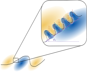
Conceptual model of the streamwise velocity fluctuations, with a detail on the smaller structures deforming the interface between positive (yellow) and negative (blue) fluctuations. Solid black lines denote the contours of the full velocity field and red dashed lines the locations where high MP deflections would be expected. An alternating sequence of positive and negative MP deflections is assumed here, with the corresponding velocity field reflecting the observations in figures 6(a) and 7(a).

Combining the main points from the above discussion, a conceptual model of the streamwise fluctuating velocity structure is proposed (see figure 14). The model complements the ideas on the small-scale $v$ structure organisation from Saxton-Fox et al. (Reference Saxton-Fox, McKeon and Gordeyev2019), expanding upon the average behaviour for the corresponding $u$ structures. In particular, the angle $\unicode[STIX]{x1D719}_{d}$ of downstream leaning velocity contours (as defined in § 3) is representative of the slope of the large-scale structures (denoted with purple solid line in figure 14). The average angle of the upstream leaning contours $\unicode[STIX]{x1D719}_{u}$ on the other hand, is a measure of the slope of the superimposed smaller-scale structures (solid cyan line). Based on the resulting streamwise velocity gradient of the small scales, an alternating sequence of high-amplitude negative and positive MP deflection events would be triggered (each denoted with a red dashed line). The full velocity contour (solid black line in figure 14) would be appropriately corrugated, following a constructive or destructive superposition of the wall-normal gradient of the mean and the fluctuating part of the velocity signal (see also McKeon Reference McKeon2017; Saxton-Fox & McKeon Reference Saxton-Fox and McKeon2017). It should be stressed again that, the ideas discussed here pertain exclusively to the organisation of velocity structures; despite the similarity expected between streamwise velocity and scalar fields (Fulachier & Dumas Reference Fulachier and Dumas1976; Kim & Moin Reference Kim and Moin1989; Antonia et al. Reference Antonia, Abe and Kawamura2009; Li et al. Reference Li, Schlatter, Brandt and Henningson2009), the present measurements do not allow direct assessment of such analogies and can only provide tentative links between regions of large scalar gradients and statistically important velocity structures.

Returning to the comparison between cold-wire measurements and the MP set-up, another point that can be discussed is the spatial extent of the observed structures. Falco (Reference Falco1977) using visualisations and temporal signals of velocity, estimated the average size of the typical eddy to be between $0.08\unicode[STIX]{x1D6FF}$ and $0.3\unicode[STIX]{x1D6FF}$. Similar extents were found by Antonia et al. (Reference Antonia, Rajagopalan, Subramanian and Chambers1982) from the shape of the conditional jumps in the velocity signals (assuming a convection velocity equal to the free-stream value). More importantly these authors showed that these extents did not vary with wall-normal location, in line with the conclusions of this study, mainly with respect to the extent of the $v$ structures (see figure 9) which are more homogeneous across $y$ and their extent more easily estimated. These observations indicate that, despite the preferential detection of the large-scale downstream inclined interfaces in the case of most point-wise measurements (${\sim}1.6$–$2.5\unicode[STIX]{x1D6FF}$ in length according to Falco (Reference Falco1977) and Chen & Blackwelder (Reference Chen and Blackwelder1978)), the extent of the jumps observed in the velocity fields highlight the presence of much smaller structures (of the order of $0.1\unicode[STIX]{x1D6FF}$), in agreement with the results in the present work.

Finally, a note should be made regarding the skewness $S$ of the MP signal. In the present study $S$ was found to be negative with a small but non-zero magnitude, $|S|=0.12$ (slightly lower than the value $|S|=0.22$ found by Saxton-Fox Reference Saxton-Fox2018), in line with the prominence of very-large-magnitude negative MP events (see figure 13b). As was mentioned before, the MP signal is proportional to the temporal variation of the streamwise density gradient (see (2.2)). Taking into account the ideal gas law, this would indicate a non-zero (positive) skewness of the temperature gradient, an observation repeated in numerous studies of passive scalar transport and thoroughly analysed, mainly in the context of local isotropy (Mestayer et al. (Reference Mestayer, Gibson, Coantic and Patel1976), Gibson et al. (Reference Gibson, Friehe and McConnell1977), Sreenivasan & Antonia (Reference Sreenivasan and Antonia1977), Antonia & Van Atta (Reference Antonia and Van Atta1978) and Sreenivasan (Reference Sreenivasan2018), among others). The absolute values of skewness in these studies were significantly higher than the one documented here. However, a quantitative comparison is not appropriate since the signal measured by the MP is only proportional to the density gradient, while in the aforementioned studies skewness is computed from point-wise temperature measurements.

6 Conclusions

Simultaneous particle image velocimetry and MP measurements were performed in a moderately heated turbulent boundary layer, where temperature acted as a passive scalar. The MP deflection signal provided a measure for the density gradient, integrated across $\unicode[STIX]{x1D6FF}$. Velocity fluctuations conditioned on large MP deflections revealed a clear change in sign for both streamwise and wall-normal velocities, consistent throughout the boundary layer height, and dependent on the sign of the MP deflection. In an effort to determine which scales contributed to this average behaviour, velocity fluctuations that were more strongly correlated with it were identified and shown to be localised in $y$.

The emerging picture for the organisation of the velocity fluctuations is that of a multiscale phenomenon, where small-scale velocity structures are superimposed on large downstream leaning outer layer motions. This is in agreement with previous observations of multiple velocity scales involved in shear layers (Klewicki & Hirschi Reference Klewicki and Hirschi2004) and is complimentary to the conceptual model proposed by Saxton-Fox et al. (Reference Saxton-Fox, McKeon and Gordeyev2019); the present work provides insight into the geometrical characteristics of both streamwise and wall-normal small-scale velocity fluctuations. The small-scale $v$ fluctuations are shown to have an average wall-normal extent ${\sim}0.1\unicode[STIX]{x1D6FF}$, almost constant across $y$, and an overall elliptical geometry. More interestingly, the corresponding small-scale $u$ fluctuations exhibit a sign change across upstream leaning interfaces with an average angle $\unicode[STIX]{x1D719}_{u}=145^{\circ }$ with respect to the horizontal. The signature of a large-scale, downstream leaning structure, consistent with the back of turbulent bulges, is also present in the conditional fields with an average angle $\unicode[STIX]{x1D719}_{u}=20^{\circ }$. The underlying flow topologies in the current study for positive and negative MP deflections are also in excellent agreement with those from earlier cold-wire studies for heatings and coolings, respectively (Antonia & Fulachier Reference Antonia and Fulachier1989), despite the very different nature of the two measurement techniques.

The integral nature of the density gradient measurements and the lack of spanwise velocity information are clear limitations of the current work and important directions for future research. However, the results herein indicate that for a great range of applications where detailed information on the scalar is not available and velocity information limited, aero-optic measurements can still provide a viable alternative for obtaining insights into the flow structure, while reducing complexity and cost of the set-up. Indeed, incorporating the observations from the current study allowed the proposal of a conceptual model for the flow organisation (figure 14), consistent with earlier cold-wire results (Antonia & Fulachier Reference Antonia and Fulachier1989), concepts of ‘typical eddies’ (Falco Reference Falco1977), as well the ideas of the hairpin packet model (Adrian et al. Reference Adrian, Meinhart and Tomkins2000). Besides, the imposed limitations of the set-up provided a natural shift in focus towards velocity features that exhibited the most robust correlation with large scalar gradients – namely gradients of the wall-normal velocity. These highlighted new geometrical aspects of the corresponding streamwise velocity fluctuations, which otherwise would have been harder to identify.

Acknowledgement

The support of the Office of Naval Research under award N00014-17-1-3022 is gratefully acknowledged.

Declaration of interests

The authors report no conflict of interest.

References

Abe, H., Antonia, R. A. & Kawamura, H. 2009 Correlation between small-scale velocity and scalar fluctuations in a turbulent channel flow. J. Fluid Mech. 627, 1–32.CrossRef Google Scholar

Adrian, R. J., Meinhart, C. D. & Tomkins, C. D. 2000 Vortex organization in the outer region of the turbulent boundary layer. J. Fluid Mech. 422, 1–54.CrossRef Google Scholar

Antonia, R. A., Abe, H. & Kawamura, H. 2009 Analogy between velocity and scalar fields in a turbulent channel flow. J. Fluid Mech. 628, 241–268.CrossRef Google Scholar

Antonia, R. A., Chambers, A. J., Friehe, C. A. & Van Atta, C. W. 1979 Temperature ramps in the atmospheric surface layer. J. Atmos. Sci. 36 (1), 99–108.2.0.CO;2>CrossRef Google Scholar

Antonia, R. A. & Fulachier, L. 1989 Topology of a turbulent boundary layer with and without wall suction. J. Fluid Mech. 198, 429–451.CrossRef Google Scholar

Antonia, R. A., Fulachier, L., Krishnamoorthy, L. V., Benabid, T. & Anselmet, F. 1988a Influence of wall suction on the organized motion in a turbulent boundary layer. J. Fluid Mech. 190, 217–240.CrossRef Google Scholar

Antonia, R. A., Krishnamoorthy, L. V. & Fulachier, L. 1988b Correlation between the longitudinal velocity fluctuation and temperature fluctuation in the near-wall region of a turbulent boundary layer. Intl J. Heat Mass Transfer 31 (4), 723–730.CrossRef Google Scholar

Antonia, R. A., Rajagopalan, S., Subramanian, C. S. & Chambers, A. J. 1982 Reynolds-number dependence of the structure of a turbulent boundary layer. J. Fluid Mech. 121, 123–140.CrossRef Google Scholar

Antonia, R. A. & Van Atta, C. W. 1978 Structure functions of temperature fluctuations in turbulent shear flows. J. Fluid Mech. 84 (3), 561–580.CrossRef Google Scholar

Antonia, R. A. & Van Atta, C. W. 1979 Skewness of spatial derivatives of temperature in a turbulent boundary layer. Phys. Fluids 22 (12), 2430–2431.CrossRef Google Scholar

Baars, W. J., Hutchins, N. & Marusic, I. 2017 Reynolds number trend of hierarchies and scale interactions in turbulent boundary layers. Phil. Trans. R. Soc. Lond. A 375 (2089), 20160077.Google Scholar PubMed

Balakumar, B. J. & Adrian, R. J. 2007 Large- and very-large-scale motions in channel and boundary-layer flows. Phil. Trans. Math. Phys. Engng Sci. 365 (1852), 665–681.CrossRef Google Scholar PubMed

Bisset, D. K., Antonia, R. A. & Raupach, M. R. 1991 Topology and transport properties of large scale organized motion in a slightly heated rough wall boundary layer. Phys. Fluids A 3 (9), 2220–2228.CrossRef Google Scholar

Chen, C.-H. P. & Blackwelder, R. F. 1978 Large-scale motion in a turbulent boundary layer: a study using temperature contamination. J. Fluid Mech. 89, 1–31.CrossRef Google Scholar

Clauser, F. H. 1954 Turbulent boundary layers in adverse pressure gradients. J. Aeronaut. Sci. 21 (2), 91–108.CrossRef Google Scholar

De Graaff, D. B. & Eaton, J. K. 2000 Reynolds-number scaling of the flat-plate turbulent boundary layer. J. Fluid Mech. 422, 319–346.CrossRef Google Scholar

Falco, R. E. 1977 Coherent motions in the outer region of turbulent boundary layers. Phys. Fluids 20 (10), S124–S132.CrossRef Google Scholar

Fulachier, L. & Dumas, R. 1976 Spectral analogy between temperature and velocity fluctuations in a turbulent boundary layer. J. Fluid Mech. 77 (2), 257–277.CrossRef Google Scholar

Gibson, C. H., Friehe, C. A. & McConnell, S. O. 1977 Structure of sheared turbulent fields. Phys. Fluids 20 (10), S156–S167.CrossRef Google Scholar

Gladstone, J. H. & Dale, T. P. 1862 Researches on the refraction, dispersion, and sensitiveness of liquids. Proc. R. Soc. Lond. 12, 448–453.Google Scholar

Gordeyev, S., Cress, J. A., Smith, A. E. & Jumper, E. J. 2015 Aero-optical measurements in a subsonic, turbulent boundary layer with non-adiabatic walls. Phys. Fluids 27 (4), 045110.CrossRef Google Scholar

Gordeyev, S., Hayden, T. E. & Jumper, E. J. 2007 Aero-optical and flow measurements over a flat-windowed turret. AIAA J. 45 (2), 347–357.CrossRef Google Scholar

Gordeyev, S., Jumper, E. J., Ng, T. T. & Cain, A. B.2003 Aero-optical characteristics of compressible, subsonic turbulent boundary layers. AIAA Paper 2003-3606.Google Scholar

Gordeyev, S. & Smith, A. E.2016 Studies of the large-scale structure in turbulent boundary layers using simultaneous velocity-wavefront measurements. AIAA Paper 2016-3804.CrossRef Google Scholar

Gordeyev, S., Smith, A. E., Cress, J. A. & Jumper, E. J. 2014 Experimental studies of aero-optical properties of subsonic turbulent boundary layers. J. Fluid Mech. 740, 214–253.CrossRef Google Scholar

Guala, M., Hommema, S. E. & Adrian, R. J. 2006 Large-scale and very-large-scale motions in turbulent pipe flow. J. Fluid Mech. 554, 521–542.CrossRef Google Scholar

Head, M. R. & Bandyopadhyay, P. 1981 New aspects of turbulent boundary-layer structure. J. Fluid Mech. 107, 297–338.CrossRef Google Scholar

Hutchins, N. & Marusic, I. 2007 Large-scale influences in near-wall turbulence. Phil. Trans. R. Soc. Lond. A 365 (1852), 647–664.CrossRef Google Scholar PubMed

Jumper, E. J. & Gordeyev, S. 2017 Physics and measurement of aero-optical effects: past and present. Annu. Rev. Fluid Mech. 49 (1), 419–441.CrossRef Google Scholar

Kim, J. & Moin, P. 1989 Transport of passive scalars in a turbulent channel flow. In Turbulent Shear Flows 6, pp. 85–96. Springer.CrossRef Google Scholar

Klewicki, J. C. & Hirschi, C. R. 2004 Flow field properties local to near-wall shear layers in a low Reynolds number turbulent boundary layer. Phys. Fluids 16 (11), 4163–4176.CrossRef Google Scholar

Li, Q., Schlatter, P., Brandt, L. & Henningson, D. S. 2009 DNS of a spatially developing turbulent boundary layer with passive scalar transport. Intl J. Heat Fluid Flow 30 (5), 916–929.CrossRef Google Scholar

Lozano-Duran, A., Flores, O. & Jimenez, J. 2012 The three-dimensional structure of momentum transfer in turbulent channels. J. Fluid Mech. 694, 100–130.CrossRef Google Scholar

Malley, M. M., Sutton, G. W. & Kincheloe, N. 1992 Beam-jitter measurements of turbulent aero-optical path differences. Appl. Opt. 31, 4440–4443.CrossRef Google Scholar PubMed

Mathis, R., Hutchins, N. & Marusic, I. 2009 Large-scale amplitude modulation of the small-scale structures in turbulent boundary layers. J. Fluid Mech. 628, 311–337.CrossRef Google Scholar

McKeon, B. J. 2017 The engine behind (wall) turbulence: perspectives on scale interactions. J. Fluid Mech. 817, P1.CrossRef Google Scholar

Mestayer, P. G., Gibson, C. H., Coantic, M. F. & Patel, A. S. 1976 Local anisotropy in heated and cooled turbulent boundary layers. Phys. Fluids 19 (9), 1279–1287.CrossRef Google Scholar

Morkovin, M. V. 1962 Effects of compressibility on turbulent flows. In Mechanique de la Turbulence (ed. Favre, A.), pp. 367–380. CNRS.Google Scholar

Saxton-Fox, T.2018 Coherent structures, their interactions, and their effects on passive scalar transport and aero-optic distortion in a turbulent boundary layer. PhD thesis, California Institute of Technology, Pasadena, CA.Google Scholar

Saxton-Fox, T. & McKeon, B. J. 2017 Coherent structures, uniform momentum zones and the streamwise energy spectrum in wall-bounded turbulent flows. J. Fluid Mech. 826, R6.CrossRef Google Scholar

Saxton-Fox, T., McKeon, B. J. & Gordeyev, S. 2019 Effect of coherent structures on aero-optic distortion in a turbulent boundary layer. AIAA J. 57 (7), 2828–2839.CrossRef Google Scholar

Saxton-Fox, T., McKeon, B. J., Gordeyev, S. & Smith, A. E. 2015 Aero-optical distortion as a marker of turbulent structure. In 11th International Symposium on Particle Image Velocimetry, Santa Barbara, CA.Google Scholar

de Silva, C. M., Kevin, K., Baidya, R., Hutchins, N. & Marusic, I. 2018 Large coherence of spanwise velocity in turbulent boundary layers. J. Fluid Mech. 847, 161–185.CrossRef Google Scholar

de Silva, C. M., Philip, J., Hutchins, N. & Marusic, I. 2017 Interfaces of uniform momentum zones in turbulent boundary layers. J. Fluid Mech. 820, 451–478.CrossRef Google Scholar

Smith, A. E., Gordeyev, S., Saxton-Fox, T. & McKeon, B. J.2014 Subsonic boundary-layer wavefront spectra for a range of Reynolds numbers. AIAA Paper 2014-2491.CrossRef Google Scholar

Smits, A. J. & Dussuage, J.-P. 2006 Turbulent Shear Layers in Supersonic Flow. Springer.Google Scholar

Spalding, D. B. 1961 A single formula for the law of the wall. J. Appl. Mech. 28 (3), 455–458.CrossRef Google Scholar

Sreenivasan, K. R. 2018 Turbulent mixing: a perspective. Proc. Natl Acad. Sci. USA 116 (37), 18175–18183.CrossRef Google Scholar PubMed

Sreenivasan, K. R. & Antonia, R. A. 1977 Skewness of temperature derivatives in turbulent shear flows. Phys. Fluids 20 (12), 1986–1988.CrossRef Google Scholar

Subramanian, C. S., Rajagopalan, S., Antonia, R. A. & Chambers, A. J. 1982 Comparison of conditional sampling and averaging techniques in a turbulent boundary layer. J. Fluid Mech. 123, 335–362.CrossRef Google Scholar

Theodorsen, T. 1952 Mechanism of turbulence. In Proceedings of the Midwestern Conference on Fluid Mechanics, Ohio State University, Columbus, OH.Google Scholar

Vanderwel, C. & Tavoularis, S. 2016 Scalar dispersion by coherent structures in uniformly sheared flow generated in a water tunnel. J. Turbul. 17 (7), 633–650.CrossRef Google Scholar

Wang, K. & Wang, M. 2012 Aero-optics of subsonic turbulent boundary layers. J. Fluid Mech. 696, 122–151.CrossRef Google Scholar

Wang, M., Mani, A. & Gordeyev, S. 2012 Physics and computation of aero-optics. Annu. Rev. Fluid Mech. 44 (1), 299–321.CrossRef Google Scholar

Figure 1.Experimental set-up. (a) Side view of the plate. (b) Perspective view of the complete configuration. (c) Enlarged view of the measurement location including the PIV laser sheet and the MP laser beam path.

Figure 2.For $\unicode[STIX]{x2202}\unicode[STIX]{x1D70C}/\unicode[STIX]{x2202}x<0$ the beam experiences an upstream deflection regardless of the angle $\unicode[STIX]{x1D6FC}$, between the density front and the horizontal. Upstream leaning density front, $\unicode[STIX]{x2202}\unicode[STIX]{x1D70C}/\unicode[STIX]{x2202}y<0$, $\unicode[STIX]{x1D6FC}<\unicode[STIX]{x03C0}/2$ (a), downstream leaning density front, $\unicode[STIX]{x2202}\unicode[STIX]{x1D70C}/\unicode[STIX]{x2202}y>0$, $\unicode[STIX]{x1D6FC}>\unicode[STIX]{x03C0}/2$ (b). Warm and cool colours indicate higher and lower values for the density, respectively.

Figure 3.(a) Inner-normalised streamwise mean velocity. Inner-normalised r.m.s. values of streamwise (b), wall-normal velocity intensities (c) and Reynolds shear stress (d). Present data are compared with results from De Graaff & Eaton (2000) at similar Reynolds numbers.

Table 1.Nominal flow conditions.

Figure 4.Contour plots of inner-normalised velocity fluctuations and their outer-normalised streamwise gradients, conditionally averaged on the MP deflection angle (negative deflection on the left and positive on the right for all panels). Black dashed lines indicate the MP location. Streamwise velocity fluctuations (a), and the corresponding streamwise gradient (c). Wall-normal velocity fluctuations (b), and the corresponding streamwise gradient (d).

Table 2.Percentage of frames and parameters for the Gaussian function $s_{G1}$, for both negative and positive large MP deflections.

Figure 5.(a,b) Wall-normal average of the contour plots in figure 4(d) for a negative and positive MP deflection, respectively. Solid lines denote the Gaussian approximation of the profile, $s_{G1}$, for increasing peak width, $c^{\ast }$, and symbols denote $s_{1}$. (c) Instantaneous profile of $\unicode[STIX]{x1D70C}_{s_{1},s_{2}}$. Red dotted line indicates the location, $y_{c}$, where $\unicode[STIX]{x1D70C}_{s_{1},s_{2}}$ is maximum. (d,e) Probability density function of $y_{c}$ for negative and positive MP deflections, respectively. Coloured bars denote $s_{1}$ and solid lines its Gaussian approximation, $s_{G1}$, for increasing peak width, $c^{\ast }$. (f) Average profile of the correlation coefficient $\unicode[STIX]{x1D70C}_{s_{1},s_{2}}=\langle \unicode[STIX]{x1D70C}_{s_{1},s_{2i}}\rangle$ for different values of $c^{\ast }$.

Figure 6.Contour plots of inner-normalised velocity fluctuations, conditionally averaged on both a negative MP deflection angle ($\unicode[STIX]{x1D703}<-0.5\unicode[STIX]{x1D70E}_{\unicode[STIX]{x1D703}}$) and on $y_{c}$. The five panels are, from left to right: $y_{c}\in [0,0.2\unicode[STIX]{x1D6FF})$, $y_{c}\in [0.2\unicode[STIX]{x1D6FF},0.4\unicode[STIX]{x1D6FF})$, $y_{c}\in [0.4\unicode[STIX]{x1D6FF},0.6\unicode[STIX]{x1D6FF})$, $y_{c}\in [0.6\unicode[STIX]{x1D6FF},0.8\unicode[STIX]{x1D6FF})$ and $y_{c}\in [0.8\unicode[STIX]{x1D6FF},1.0\unicode[STIX]{x1D6FF})$. Vertical dashed lines denote the MP location. (a) Streamwise velocity fluctuations. (b) Wall-normal velocity. (c) Streamlines using the full velocity field and subtracting $U_{c}=\langle U(x,y_{cm})\rangle _{x}$, indicating that $\unicode[STIX]{x2202}\unicode[STIX]{x1D70C}/\unicode[STIX]{x2202}x<0$ events are aligned with diverging separatrices, going through saddle points, in line with observations from Antonia & Fulachier (1989) on coolings.

Figure 7.Contour plots of inner-normalised velocity fluctuations, conditionally averaged on both a positive MP deflection angle ($\unicode[STIX]{x1D703}>0.5\unicode[STIX]{x1D70E}_{\unicode[STIX]{x1D703}}$) and on $y_{c}$. The Gaussian approximation $s_{G1}$ was used for the computation of $\unicode[STIX]{x1D70C}_{s_{1},s_{2}}$, with $c^{\ast }=c$. The five panels are, from left to right: $y_{c}\in [0,0.2\unicode[STIX]{x1D6FF})$, $y_{c}\in [0.2\unicode[STIX]{x1D6FF},0.4\unicode[STIX]{x1D6FF})$, $y_{c}\in [0.4\unicode[STIX]{x1D6FF},0.6\unicode[STIX]{x1D6FF})$, $y_{c}\in [0.6\unicode[STIX]{x1D6FF},0.8\unicode[STIX]{x1D6FF})$ and $y_{c}\in [0.8\unicode[STIX]{x1D6FF},1.0\unicode[STIX]{x1D6FF})$. Vertical dashed lines denote the MP location. (a) Streamwise velocity fluctuations. (b) Wall-normal velocity. (c) Streamlines using the full velocity field and subtracting $U_{c}=\langle U(x,y_{cm})\rangle _{x}$, indicating that $\unicode[STIX]{x2202}\unicode[STIX]{x1D70C}/\unicode[STIX]{x2202}x>0$ events are aligned with unstable foci, in line with observations from Antonia & Fulachier (1989) on heatings.

Figure 8.Geometrical characteristics for $\langle v^{+}|_{\unicode[STIX]{x1D703},y_{c}}\rangle$ (figures 6–7). (a) Elliptical fits for the conditionally averaged wall-normal velocity fluctuation contours from figures 6 and 7 at 40 % of the peak magnitude and for all $y_{c}$ locations: $y_{c}\in [0,0.2\unicode[STIX]{x1D6FF})$, $y_{c}\in [0.2\unicode[STIX]{x1D6FF},0.4\unicode[STIX]{x1D6FF})$,$y_{c}\in [0.4\unicode[STIX]{x1D6FF},0.6\unicode[STIX]{x1D6FF})$, $y_{c}\in [0.6\unicode[STIX]{x1D6FF},0.8\unicode[STIX]{x1D6FF})$ and $y_{c}\in [0.8\unicode[STIX]{x1D6FF},1.0\unicode[STIX]{x1D6FF})$. (b) Variation of the peak magnitude, $\max |\langle v^{+}|_{\unicode[STIX]{x1D703},y_{c}}\rangle |$ with $y_{cm}$. Colours from darker to lighter for increasing $c^{\ast }=0.5c,1c,2c$. Solid lines in (a) and (b) denote a negative MP deflection, and dashed lines a positive one. Negative velocity fluctuations are denoted by blue while positive ones with red. (c) Here, $\unicode[STIX]{x1D6EC}_{x}$ and $\unicode[STIX]{x1D6EC}_{y}$ denote the streamwise and wall-normal extent of the elliptical contours, respectively, while $X_{e}$ and $Y_{e}$ are the coordinates of their centres.

Figure 9.Variation with $y_{cm}$ for the streamwise and wall-normal extent, $\unicode[STIX]{x1D6EC}_{x}$ and $\unicode[STIX]{x1D6EC}_{y}$ and the centroid coordinates, $X_{e}$ and $Y_{e}$, of the elliptical fits of the wall-normal velocity fluctuations (defined in figure 8c). In all panels, transition from darker to lighter colours (highlighted with arrows) indicates an increasing peak width ($c^{\ast }=0.5c,1c,2c$) for $s_{G1}$ (3.4). (a,d) $\unicode[STIX]{x1D6EC}_{x}$ and $\unicode[STIX]{x1D6EC}_{y}$ for $\langle v^{+}|_{\unicode[STIX]{x1D703},y_{c}}\rangle >0$. (b,e) $\unicode[STIX]{x1D6EC}_{x}$ and $\unicode[STIX]{x1D6EC}_{y}$ for $\langle v^{+}|_{\unicode[STIX]{x1D703},y_{c}}\rangle <0$. Solid lines for a negative MP deflection and dashed for a positive one. (c,f) $X_{e}$ and $Y_{e}$ for a negative MP deflection.

Figure 10.Contours of inner-normalised vertical velocity fluctuations, $\langle v^{+}|_{\unicode[STIX]{x1D703},y_{c}}\rangle$, at 30 % of their peak magnitude, conditionally averaged on both a large MP deflection and on $y_{c}$ (from figures 6b and 7b), supporting the conceptual schematic proposed by Saxton-Fox et al. (2019); $\unicode[STIX]{x1D703}<-0.5\unicode[STIX]{x1D70E}_{\unicode[STIX]{x1D703}}$ (a), $\unicode[STIX]{x1D703}>0.5\unicode[STIX]{x1D70E}_{\unicode[STIX]{x1D703}}$ (b).

Figure 11.Contour plots of inner-normalised streamwise velocity fluctuations, conditionally averaged on the MP deflection angle, the wall-normal location $y_{c}$ ( $y_{c}\in [0.4\unicode[STIX]{x1D6FF},0.6\unicode[STIX]{x1D6FF})$) and the sign of $c_{\unicode[STIX]{x1D719}}=(\unicode[STIX]{x2202}u/\unicode[STIX]{x2202}x)(\unicode[STIX]{x2202}u/\unicode[STIX]{x2202}y)|_{x_{MP},y_{c}}$ (3.5). For both images: $\unicode[STIX]{x1D703}<-0.5\unicode[STIX]{x1D70E}_{\unicode[STIX]{x1D703}}$ (left), $\unicode[STIX]{x1D703}>0.5\unicode[STIX]{x1D70E}_{\unicode[STIX]{x1D703}}$ (right). (a) For a downstream leaning contour ($\unicode[STIX]{x1D719}_{d}$, solid purple lines), $c^{\ast }=2c$. (b) For an upstream leaning contour ($\unicode[STIX]{x1D719}_{u}$), $c^{\ast }=0.5c$ (solid cyan lines on the right).

Figure 12.Characteristics for $\langle u^{+}|_{\unicode[STIX]{x1D703},y_{c},\unicode[STIX]{x1D719}}\rangle =0$ contours. Solid and dashed lines indicate a negative and positive MP deflection, respectively. Grey lines in (a–c) denote linear fits and dashed vertical lines the MP location. (a) Variation with wall-normal location for $\unicode[STIX]{x1D719}=\unicode[STIX]{x1D719}_{d}$ and $c^{\ast }=2c$. (b) Variation with wall-normal location for $\unicode[STIX]{x1D719}=\unicode[STIX]{x1D719}_{u}$ and $c^{\ast }=0.5c$. (c) The angles $\unicode[STIX]{x1D719}_{u}$ and $\unicode[STIX]{x1D719}_{d}$ of the linear fits in (a) and (b) are defined with respect to the horizontal. (d) Percentage of events where $c_{\unicode[STIX]{x1D719}}>0$ ($\unicode[STIX]{x1D719}=\unicode[STIX]{x1D719}_{u}$) and $c_{\unicode[STIX]{x1D719}}<0$ ($\unicode[STIX]{x1D719}=\unicode[STIX]{x1D719}_{d}$) with respect to the total number of events, per wall-normal location. Colours as in (a–c). A transition from darker to lighter colours indicates an increasing peak width ($c^{\ast }=0.5c,1c,2c$) for $s_{G1}$ (3.4). (e) Variation of the angles $\unicode[STIX]{x1D719}_{u}$ and $\unicode[STIX]{x1D719}_{d}$ as defined in (c), per wall-normal location.

Figure 13.Temporal characteristics of large magnitude MP events. (a) Segment of time signal of the MP deflection $\unicode[STIX]{x1D703}$. Squares denote positive (gold) and negative (green) large-scale events. (b) Variation of the relative number of positive and negative MP deflection events with increasing threshold $w=|\unicode[STIX]{x1D703}|/\unicode[STIX]{x1D70E}_{\unicode[STIX]{x1D703}}$. (c) Variation of the average period, $\overline{T}_{\unicode[STIX]{x1D703}\unicode[STIX]{x1D703}}$ between two successive negative or positive events with $w$.

Figure 14.Conceptual model of the streamwise velocity fluctuations, with a detail on the smaller structures deforming the interface between positive (yellow) and negative (blue) fluctuations. Solid black lines denote the contours of the full velocity field and red dashed lines the locations where high MP deflections would be expected. An alternating sequence of positive and negative MP deflections is assumed here, with the corresponding velocity field reflecting the observations in figures 6(a) and 7(a).

Article contents

Spatial organisation of velocity structures for large passive scalar gradients

Abstract

JFM classification

Information

1 Introduction

2 Methodology

2.1 Aero-optic measurements

2.2 Velocity measurements

2.3 Large magnitude MP deflections

3 Results

3.1 Vertical velocity

3.2 Streamwise velocity

4 Time scales of large MP deflections

5 Discussion

6 Conclusions

Acknowledgement

Declaration of interests

References

Save article to Kindle

Save article to Dropbox

Save article to Google Drive

Reply to: Submit a response

Your details

You have entered the maximum number of contributors

Conflicting interests