1 Introduction
The need to reduce CO2 emissions is transforming the energy-related sectors; new methods of production and waste heat recovery are under development to achieve the required reduction targets. Similarly much research in recent years has focused on recovering waste heat and harnessing renewable energy sources. Among the possible technologies, the thermoacoustic device is unique in terms of its flexibility, reliability and affordability. Any external heat (solar energy, combustion, exhaust gas, hot liquid) can be supplied to the system via heat exchangers. The need of any moving parts, such as pistons, shafts and turbo-machines, is eliminated thereby minimizing friction, lubrication and wear. Thermoacoustic devices also have a simple structure which leads to fewer parts, ease of assembly and consequently low construction costs. In addition, thermoacoustic devices typically use noble gases as working fluid; these gases are environmentally friendly and cause no greenhouse effects.
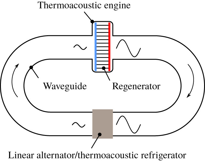
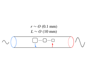
Thermoacoustic devices in this paper refer to any cyclic devices which make use of the interaction between acoustic waves and solid boundaries with a temperature gradient. In place of mechanical components, the acoustic waves provide the necessary compression and expansion processes and drive a fluid to oscillate. As the fluid moves back and forth over the imposed spatial temperature difference, it absorbs and rejects heat from and to the solid walls. Depending on the sequence of heat transfer and pressure/volume change, a thermoacoustic device can accomplish either power generation or refrigeration. When the acoustic waves are externally supplied, for example by a loudspeaker, the device operates as a thermoacoustic refrigerator (e.g. Poese & Garrett Reference Poese and Garrett2000; Bassem, Ueda & Akisawa Reference Bassem, Ueda and Akisawa2011) where acoustic work is consumed to transport heat against a temperature increase. If the temperature gradient is externally imposed, the device operates as a thermoacoustic engine (Backhaus & Swift Reference Backhaus and Swift1999; Tijani & Spoelstra Reference Tijani and Spoelstra2011) where the acoustic waves are spontaneously excited by the net heat input. The acoustic waves can be used for electricity generation if the engine is coupled with a linear alternator (Yu, Jaworski & Backhaus Reference Yu, Jaworski and Backhaus2012) or driving a thermoacoustic refrigerator, completing a heat–acoustic–cool conversion (Dai et al. Reference Dai, Luo, Zhang and Ling2006). A schematic diagram of a typical travelling-wave thermoacoustic energy system is shown in figure 1. The amplified waveform after going through the thermoacoustic engine indicates the conversion from thermal to acoustic energy. The diminished waveform indicates the consumption of acoustic energy by output devices such as a linear alternator or thermoacoustic refrigerator. Figure 1 also shows that the regenerator consists of numerous narrow flow channels. This paper concerns the disturbance energy conservation in one single regenerator channel.
A schematic diagram of a typical travelling-wave thermoacoustic energy system. The blue and red strips denote cold and hot heat exchangers, respectively. Arrows denote the direction in which the waves propagate.

Thermoacoustics as a physical process occurs in various systems with a variety of characteristics, but the conversion between thermal and acoustic energy is always central to the phenomenon. In combustion systems like gas turbine engines, the thermoacoustic combustion instability is a major issue (Lieuwen & Yang Reference Lieuwen and Yang2005). The thermal energy from unsteady heat release amplifies acoustic waves (Dowling & Stow Reference Dowling and Stow2003), which causes damage. On the contrary, in thermoacoustic devices, the conversion is purposefully encouraged as much as possible. The conversion happens in the component called the regenerator or stack which consists of many small channels; the energy conversion is therefore subtle and complex due to the interaction of oscillations, viscosity and heat transfer. It is worth noting that often the modelling of thermoacoustic processes is approximated using a heat transfer term and a drag term (Karpov & Prosperetti Reference Karpov and Prosperetti2002; Scalo, Lele & Hesselink Reference Scalo, Lele and Hesselink2015); although these terms help to model the system dynamics, the empirical method provides limited new insights into the energy conversion. The direct solution of energy conversion, in perturbation theory, requires the evaluation of at least second-order terms. Merkli & Thomann (Reference Merkli and Thomann1975) first found that in order to determine the second-order time-averaged wall heat flux, only the linear solutions of temperature and axial velocity oscillation were needed. They gave an analytical expression of heat flux to the wall for a constant temperature in a resonance tube. The results showed that the local wall heat flux equals the axial change of cross-sectional enthalpy flux due to oscillation. This idea has been further developed by Rott (Reference Rott1975), who included a temperature gradient on the wall.
Another approach to analyse the energy balance in thermoacoustic devices is to use the sum of all energy flux density, which is a conserved quantity for periodic oscillation (Cao et al. Reference Cao, Olson, Swift and Chen1996). The energy balance was explained as the conversion between acoustic intensity and the product of mean density, mean temperature and local entropy flux (Swift Reference Swift1988; Tominaga Reference Tominaga1995) which was loosely termed ‘thermoacoustic heat flux’. Although this theory could explain the growth of acoustic intensity, it assumes that the wall is adiabatic for second-order heat flux. Also, dissipation was not included in the conversion and the role of wall temperature was not clear.
A third approach to energy analysis has been briefly mentioned by Swift (Reference Swift2002, pp. 109–111). Based on a lumped-element approach, that study discussed the axial change of acoustic intensity in two simplified cases: zero viscosity and constant wall temperature. Although the definitions of dissipation and source term are preliminary, this approach is particularly inspirational to the current study.
In other research areas, there has also been some very relevant discussion. As a pure mechanics problem, the disturbance energy conservation itself has attracted considerable interest. Chu (Reference Chu1965) recognized the role of entropy fluctuation in the definition of disturbance energy compared with acoustic energy. Myers (Reference Myers1991) has shown the disturbance energy corollary is a ‘complete, consistent representation of total fluid energy conservation’ at the leading order (second order) and it only contains first-order fluctuation quality. Building upon that work, Giauque et al. (Reference Giauque, Poinsot, Brear and Nicoud2006) extended the disturbance energy corollary to reacting flow by including a mixture of gaseous species and heat release terms.
In summary, there is a lack of rigorous theory in the literature to explain the disturbance energy budget in conditions typically found in thermoacoustic devices:
(i) extremely long and narrow tubes;
(ii) significant viscous effects;
(iii) mean temperature gradient imposed on the solid boundary; and
(iv) significant heat transfer with the wall.
More importantly, by using the disturbance energy balance, a new perspective is enabled for looking at how various parameters affect the performance and characteristics of thermoacoustic devices. This is urgently needed to make thermoacoustic devices more efficient and applicable.
This paper presents a new analytical framework by applying the disturbance energy corollary to thermoacoustic devices. A thermoacoustic production term which is directly linked to the wall temperature gradient is newly defined. In place of acoustic intensity, an extended flux term is used to account for spatial growth or decay of the energy transported by the waves. Together with viscous and thermal dissipation resulting from gradients of fluctuating velocity and temperature, the disturbance energy balance relation is then established. The analytical framework is implemented in an axisymmetric cylindrical domain. A dimensional analysis is conducted to reveal the controlling parameters, namely the Womersley, Helmholtz and Prandtl numbers. The disturbance energy terms are then simplified using order-of-magnitude analysis and taking advantage of boundary conditions. The solutions and numerical scheme are then given and a global error is defined. A parametric study of the Womersley and Helmholtz numbers demonstrates the usage of the analytical framework and provides insights into the flow physics.
2 Analytical framework
In this section, a new analytical framework for disturbance energy balance is developed, starting with linearizing and rearranging the basic governing equations. Thermoacoustic production is rigorously defined together with an extended flux term to account for the spatial disturbance energy change. With the inclusion of dissipation mechanisms, the disturbance energy balance relation is established and the physical interpretation of the terms is given in detail.
The formulation begins with the governing equations:
 $$\begin{eqnarray}\displaystyle & p=\unicode[STIX]{x1D70C}R_{g}T, & \displaystyle\end{eqnarray}$$
 $$\begin{eqnarray}\displaystyle & \displaystyle \frac{\unicode[STIX]{x2202}\unicode[STIX]{x1D70C}}{\unicode[STIX]{x2202}t}+\unicode[STIX]{x1D735}\boldsymbol{\cdot }(\unicode[STIX]{x1D70C}\boldsymbol{v})=0, & \displaystyle\end{eqnarray}$$
 $$\begin{eqnarray}\displaystyle & \displaystyle \unicode[STIX]{x1D70C}\left[\frac{\unicode[STIX]{x2202}\boldsymbol{v}}{\unicode[STIX]{x2202}t}+(\boldsymbol{v}\boldsymbol{\cdot }\unicode[STIX]{x1D735})\boldsymbol{v}\right]=-\unicode[STIX]{x1D735}p+\unicode[STIX]{x1D735}\boldsymbol{\cdot }\unicode[STIX]{x1D749}, & \displaystyle\end{eqnarray}$$
 $$\begin{eqnarray}\displaystyle & \displaystyle \unicode[STIX]{x1D70C}T\left(\frac{\unicode[STIX]{x2202}s}{\unicode[STIX]{x2202}t}+\boldsymbol{v}\boldsymbol{\cdot }\unicode[STIX]{x1D735}s\right)=\unicode[STIX]{x1D735}\boldsymbol{\cdot }k\unicode[STIX]{x1D735}T+(\unicode[STIX]{x1D749}\boldsymbol{\cdot }\unicode[STIX]{x1D735})\boldsymbol{\cdot }\boldsymbol{v}. & \displaystyle\end{eqnarray}$$
The fluid is taken as an ideal gas and the flow as laminar. In oscillatory pipe flow, three main types of flow regimes have been observed: laminar flow, disturbed laminar flow and intermittently turbulent flow (Hino, Sawamoto & Takasu Reference Hino, Sawamoto and Takasu1976; Akhavan, Kamm & Shapiro Reference Akhavan, Kamm and Shapiro1991). The intermittently turbulent flow is characterized by a sudden burst into turbulence during the decelerating phase of the cycle and the subsequent reversion to laminar flow during the accelerating phase. The transition usually depends on both the Stokes parameter (the ratio of pipe radius to Stokes-layer thickness) and the Reynolds number. The maximum Stokes parameter and diameter-based Reynolds number are calculated to be 1.2 and 190, respectively, for all cases in this study. According to the criteria given by Ohmi et al. (Reference Ohmi, Iguchi, Kakehashi and Masuda1982), the flow in this study is laminar and well away from transition.
When a disturbance is present, flow variables can be decomposed into mean values, denoted by subscript 0, and fluctuation components, denoted by prime, such as  $p=p_{0}+p^{\prime }$ and
 $\unicode[STIX]{x1D70C}=\unicode[STIX]{x1D70C}_{0}+\unicode[STIX]{x1D70C}^{\prime }$. Assuming that the mean state is quiescent and the mean pressure is homogeneous, it follows that
 $\boldsymbol{v}=\boldsymbol{v}^{\prime }$,
 $\unicode[STIX]{x1D749}=\unicode[STIX]{x1D749}^{\prime }$,
 $\unicode[STIX]{x1D735}p_{0}=0$ and
 $\unicode[STIX]{x2202}f_{0}/\unicode[STIX]{x2202}t=0$, where
 $f$ is any flow variable. When the disturbance is of a small amplitude, linear approximation applies and only the first-order terms are kept. The linearized governing equations take the form
 $$\begin{eqnarray}\displaystyle & p_{0}=\unicode[STIX]{x1D70C}_{0}R_{g}T_{0}, & \displaystyle\end{eqnarray}$$
 $$\begin{eqnarray}\displaystyle & p^{\prime }/p_{0}=\unicode[STIX]{x1D70C}^{\prime }/\unicode[STIX]{x1D70C}_{0}+T^{\prime }/T_{0}, & \displaystyle\end{eqnarray}$$
 $$\begin{eqnarray}\displaystyle & \displaystyle \frac{\unicode[STIX]{x2202}\unicode[STIX]{x1D70C}^{\prime }}{\unicode[STIX]{x2202}t}+\unicode[STIX]{x1D70C}_{0}\unicode[STIX]{x1D735}\boldsymbol{\cdot }\boldsymbol{v}^{\prime }+\boldsymbol{v}^{\prime }\boldsymbol{\cdot }\unicode[STIX]{x1D735}\unicode[STIX]{x1D70C}_{0}=0, & \displaystyle\end{eqnarray}$$
 $$\begin{eqnarray}\displaystyle & \displaystyle \unicode[STIX]{x1D70C}_{0}\frac{\unicode[STIX]{x2202}\boldsymbol{v}^{\prime }}{\unicode[STIX]{x2202}t}=-\unicode[STIX]{x1D735}p^{\prime }+\unicode[STIX]{x1D735}\boldsymbol{\cdot }\unicode[STIX]{x1D749}^{\prime }, & \displaystyle\end{eqnarray}$$
 $$\begin{eqnarray}\displaystyle & \displaystyle \unicode[STIX]{x1D70C}_{0}T_{0}\left(\frac{\unicode[STIX]{x2202}s^{\prime }}{\unicode[STIX]{x2202}t}+\boldsymbol{v}^{\prime }\boldsymbol{\cdot }\unicode[STIX]{x1D735}s_{0}\right)=k\unicode[STIX]{x1D6FB}^{2}T^{\prime }, & \displaystyle\end{eqnarray}$$
where the gradient of thermal conductivity  $(\unicode[STIX]{x1D735}k)$ is ignored. Multiplying (2.6) by
 $p^{\prime }/\unicode[STIX]{x1D70C}_{0}$, equation (2.8) by
 $T^{\prime }/T_{0}$, taking the dot product of (2.7) with
 $\boldsymbol{v}^{\prime }$ and adding them together yields
 $$\begin{eqnarray}\displaystyle \frac{\unicode[STIX]{x2202}}{\unicode[STIX]{x2202}t}\left(\frac{1}{2}\unicode[STIX]{x1D70C}_{0}{v^{\prime }}^{2}\right)+\frac{p^{\prime }}{\unicode[STIX]{x1D70C}_{0}}\frac{\unicode[STIX]{x2202}\unicode[STIX]{x1D70C}^{\prime }}{\unicode[STIX]{x2202}t}+\unicode[STIX]{x1D70C}_{0}T^{\prime }\frac{\unicode[STIX]{x2202}s^{\prime }}{\unicode[STIX]{x2202}t} & = & \displaystyle -\unicode[STIX]{x1D735}\boldsymbol{\cdot }(p^{\prime }\boldsymbol{v}^{\prime })-\frac{p^{\prime }\boldsymbol{v}^{\prime }}{\unicode[STIX]{x1D70C}_{0}}\boldsymbol{\cdot }\unicode[STIX]{x1D735}\unicode[STIX]{x1D70C}_{0}+\boldsymbol{v}^{\prime }\boldsymbol{\cdot }(\unicode[STIX]{x1D735}\boldsymbol{\cdot }\unicode[STIX]{x1D749})\nonumber\\ \displaystyle & & \displaystyle +\,\frac{T^{\prime }}{T_{0}}k\unicode[STIX]{x1D6FB}^{2}T^{\prime }-\unicode[STIX]{x1D70C}_{0}T^{\prime }\boldsymbol{v}^{\prime }\boldsymbol{\cdot }\unicode[STIX]{x1D735}s_{0}.\end{eqnarray}$$
Using Taylor’s theorem to expand thermodynamic relations  $\unicode[STIX]{x1D70C}=\unicode[STIX]{x1D70C}(p,s)$ and
 $T=T(p,s)$ around mean values and again keeping only the first-order term, yields
 $$\begin{eqnarray}\displaystyle & \displaystyle \unicode[STIX]{x1D70C}^{\prime }=\left(\frac{\unicode[STIX]{x2202}\unicode[STIX]{x1D70C}}{\unicode[STIX]{x2202}p}\right)_{0}p^{\prime }+\left(\frac{\unicode[STIX]{x2202}\unicode[STIX]{x1D70C}}{\unicode[STIX]{x2202}s}\right)_{0}s^{\prime }, & \displaystyle\end{eqnarray}$$
 $$\begin{eqnarray}\displaystyle & \displaystyle T^{\prime }=\left(\frac{\unicode[STIX]{x2202}T}{\unicode[STIX]{x2202}p}\right)_{0}p^{\prime }+\left(\frac{\unicode[STIX]{x2202}T}{\unicode[STIX]{x2202}s}\right)_{0}s^{\prime }, & \displaystyle\end{eqnarray}$$
whose coefficients can be evaluated using the definition of isentropic speed of sound  $c$, specific heat at constant pressure
 $c_{p}$, coefficient of thermal expansion
 $\unicode[STIX]{x1D6FD}$ and thermodynamic partial differential relations. The coefficients are then written as
 $$\begin{eqnarray}\left(\frac{\unicode[STIX]{x2202}\unicode[STIX]{x1D70C}}{\unicode[STIX]{x2202}p}\right)_{0}=\frac{1}{c_{0}^{2}},\quad \left(\frac{\unicode[STIX]{x2202}\unicode[STIX]{x1D70C}}{\unicode[STIX]{x2202}s}\right)_{0}=-\frac{\unicode[STIX]{x1D70C}_{0}\unicode[STIX]{x1D6FD}_{0}T_{0}}{c_{p0}},\quad \left(\frac{\unicode[STIX]{x2202}T}{\unicode[STIX]{x2202}p}\right)_{0}=\frac{\unicode[STIX]{x1D6FD}_{0}T_{0}}{\unicode[STIX]{x1D70C}_{0}c_{p0}},\quad \left(\frac{\unicode[STIX]{x2202}T}{\unicode[STIX]{x2202}s}\right)_{0}=\frac{T_{0}}{c_{p0}}.\end{eqnarray}$$
For ideal gases,  $\unicode[STIX]{x1D6FD}_{0}=1/T_{0}$. Henceforth dropping the subscript 0 in
 $c_{0}$ and
 $c_{p0}$, the equations become
 $$\begin{eqnarray}\displaystyle & \displaystyle \unicode[STIX]{x1D70C}^{\prime }=\frac{1}{c^{2}}p^{\prime }-\frac{\unicode[STIX]{x1D70C}_{0}}{c_{p}}s^{\prime }, & \displaystyle\end{eqnarray}$$
 $$\begin{eqnarray}\displaystyle & \displaystyle T^{\prime }=\frac{1}{\unicode[STIX]{x1D70C}_{0}c_{p}}p^{\prime }+\frac{T_{0}}{c_{p}}s^{\prime }. & \displaystyle\end{eqnarray}$$
Substituting (2.13) and (2.14) into the left-hand side of (2.9) (LHS) leads to
 $$\begin{eqnarray}\text{LHS}=\frac{\unicode[STIX]{x2202}}{\unicode[STIX]{x2202}t}\left(\frac{1}{2}\unicode[STIX]{x1D70C}_{0}v^{\prime 2}\right)+\frac{\unicode[STIX]{x2202}}{\unicode[STIX]{x2202}t}\left(\frac{1}{2}\frac{1}{c^{2}\unicode[STIX]{x1D70C}_{0}}p^{\prime 2}\right)+\frac{\unicode[STIX]{x2202}}{\unicode[STIX]{x2202}t}\left(\frac{1}{2}\frac{\unicode[STIX]{x1D70C}_{0}T_{0}}{c_{p}}s^{\prime 2}\right).\end{eqnarray}$$
The third and fourth terms on the right-hand side of (2.9) can be written as
 $$\begin{eqnarray}\boldsymbol{v}^{\prime }\boldsymbol{\cdot }(\unicode[STIX]{x1D735}\boldsymbol{\cdot }\unicode[STIX]{x1D749}^{\prime })=\unicode[STIX]{x1D735}\boldsymbol{\cdot }(\unicode[STIX]{x1D749}^{\prime }\boldsymbol{\cdot }\boldsymbol{v}^{\prime })-\unicode[STIX]{x1D749}^{\prime }\boldsymbol{ : }\unicode[STIX]{x1D735}\boldsymbol{v}^{\prime },\end{eqnarray}$$
 $$\begin{eqnarray}\displaystyle \frac{T^{\prime }}{T_{0}}k\unicode[STIX]{x1D6FB}^{2}T^{\prime } & = & \displaystyle \unicode[STIX]{x1D735}\boldsymbol{\cdot }\left(\frac{T^{\prime }}{T_{0}}k\unicode[STIX]{x1D735}T^{\prime }\right)-\unicode[STIX]{x1D735}T^{\prime }\boldsymbol{\cdot }\unicode[STIX]{x1D735}k\frac{T^{\prime }}{T_{0}}\nonumber\\ \displaystyle & = & \displaystyle \unicode[STIX]{x1D735}\boldsymbol{\cdot }\left(\frac{T^{\prime }}{T_{0}}k\unicode[STIX]{x1D735}T^{\prime }\right)-k\frac{\left(\unicode[STIX]{x1D735}T^{\prime }\right)^{2}}{T_{0}}+k\frac{T^{\prime }}{T_{0}^{2}}\unicode[STIX]{x1D735}T_{0}\boldsymbol{\cdot }\unicode[STIX]{x1D735}T^{\prime }.\end{eqnarray}$$
Since  $\unicode[STIX]{x1D735}p_{0}=0$, it is easy to show that
 $$\begin{eqnarray}-\frac{1}{\unicode[STIX]{x1D70C}_{0}}\unicode[STIX]{x1D735}\unicode[STIX]{x1D70C}_{0}=\frac{1}{T_{0}}\unicode[STIX]{x1D735}T_{0}=\frac{1}{c_{p}}\unicode[STIX]{x1D735}s_{0}.\end{eqnarray}$$
Substituting the above equation and rearranging,
 $$\begin{eqnarray}\displaystyle \text{RHS} & = & \displaystyle -\unicode[STIX]{x1D735}\boldsymbol{\cdot }\left(p^{\prime }\boldsymbol{v}^{\prime }-\unicode[STIX]{x1D749}^{\prime }\boldsymbol{\cdot }\boldsymbol{v}^{\prime }-\frac{T^{\prime }}{T_{0}}k\unicode[STIX]{x1D735}T^{\prime }\right)+\left(p^{\prime }-\unicode[STIX]{x1D70C}_{0}c_{p}T^{\prime }\right)\boldsymbol{v}^{\prime }\boldsymbol{\cdot }\frac{\unicode[STIX]{x1D735}T_{0}}{T_{0}}\nonumber\\ \displaystyle & & \displaystyle +\,\frac{T^{\prime }}{T_{0}}k\unicode[STIX]{x1D735}T^{\prime }\boldsymbol{\cdot }\frac{\unicode[STIX]{x1D735}T_{0}}{T_{0}}-\left(\unicode[STIX]{x1D749}^{\prime }\boldsymbol{ : }\unicode[STIX]{x1D735}\boldsymbol{v}^{\prime }+k\frac{(\unicode[STIX]{x1D735}T^{\prime })^{2}}{T_{0}}\right),\end{eqnarray}$$
where RHS is the right-hand side of (2.9). In a similar manner to that in (2.10)–(2.14), thermodynamic relation  $s=s(T,p)$ becomes
 $$\begin{eqnarray}s^{\prime }=\frac{c_{p}}{T_{0}}T^{\prime }-\frac{1}{T_{0}\unicode[STIX]{x1D70C}_{0}}p^{\prime }.\end{eqnarray}$$
After substituting the above equation into (2.19) and rearranging, equation (2.9) can be written as
 $$\begin{eqnarray}\frac{\unicode[STIX]{x2202}w}{\unicode[STIX]{x2202}t}+\unicode[STIX]{x1D735}\boldsymbol{\cdot }I=-{\mathcal{D}}_{\unicode[STIX]{x1D708}}-{\mathcal{D}}_{k}+{\mathcal{P}},\end{eqnarray}$$
where
 $$\begin{eqnarray}\displaystyle & \displaystyle w=\frac{1}{2}\unicode[STIX]{x1D70C}_{0}{v^{\prime }}^{2}+\frac{1}{2}\frac{1}{c^{2}\unicode[STIX]{x1D70C}_{0}}{p^{\prime }}^{2}+\frac{1}{2}\frac{\unicode[STIX]{x1D70C}_{0}T_{0}}{c_{p}}{s^{\prime }}^{2}, & \displaystyle\end{eqnarray}$$
 $$\begin{eqnarray}\displaystyle & \displaystyle I=p^{\prime }\boldsymbol{v}^{\prime }-\unicode[STIX]{x1D749}^{\prime }\boldsymbol{\cdot }\boldsymbol{v}^{\prime }-\frac{T^{\prime }}{T_{0}}k\unicode[STIX]{x1D735}T^{\prime }, & \displaystyle\end{eqnarray}$$
 $$\begin{eqnarray}\displaystyle & \displaystyle {\mathcal{D}}_{\unicode[STIX]{x1D708}}=\unicode[STIX]{x1D749}^{\prime }\boldsymbol{ : }\unicode[STIX]{x1D735}\boldsymbol{v}^{\prime }, & \displaystyle\end{eqnarray}$$
 $$\begin{eqnarray}\displaystyle & \displaystyle {\mathcal{D}}_{k}=k\frac{(\unicode[STIX]{x1D735}T^{\prime })^{2}}{T_{0}}, & \displaystyle\end{eqnarray}$$
 $$\begin{eqnarray}\displaystyle & \displaystyle {\mathcal{P}}=\left(\frac{T^{\prime }}{T_{0}}k\unicode[STIX]{x1D735}T^{\prime }-T_{0}\unicode[STIX]{x1D70C}_{0}s^{\prime }\boldsymbol{v}^{\prime }\right)\frac{\unicode[STIX]{x1D735}T_{0}}{T_{0}}. & \displaystyle\end{eqnarray}$$
The disturbance energy corollary (2.21) is a central contribution of the present work; it describes the disturbance energy conservation law obtained from the linearized governing equations. The term  $\unicode[STIX]{x2202}w/\unicode[STIX]{x2202}t$ is the time rate of change of disturbance energy per unit volume in a infinitesimal control volume. The term
 $I$ represents the energy transported per unit area and time on the surfaces of the infinitesimal control volume due to the fluctuation of pressure, velocity and temperature. The transport is due to the flow work (
 $p^{\prime }\boldsymbol{v}^{\prime }$), the work done by viscous stresses (
 $\unicode[STIX]{x1D749}^{\prime }\boldsymbol{\cdot }\boldsymbol{v}^{\prime }$) and the heat conduction (
 $(T^{\prime }/T_{0})k\unicode[STIX]{x1D735}T^{\prime }$). The term
 $I$ is a more general representation of the energy flux transported by waves than the commonly used acoustic energy flux or acoustic intensity (namely fluctuating flow work
 $p^{\prime }\boldsymbol{v}^{\prime }$). Hence
 $I$ is referred to as disturbance energy flux in this study to reflect this generalization, but ‘acoustic energy’ is still casually used to resonate with readers. A positive
 $\unicode[STIX]{x1D735}\boldsymbol{\cdot }I$ means more disturbance energy flows out of the control volume than flows in; hence there is a spatial increase of energy transported by the waves. In other words, there is wave growth. Similarly, a negative
 $\unicode[STIX]{x1D735}\boldsymbol{\cdot }I$ means a spatial decrease of wave energy, i.e. wave decay. Practically, there are two types of thermoacoustic device depending on the sign of
 $\unicode[STIX]{x1D735}\boldsymbol{\cdot }I$. Positive
 $\unicode[STIX]{x1D735}\boldsymbol{\cdot }I$ is the desirable output of a thermoacoustic engine, in which case the wave is amplified; negative
 $\unicode[STIX]{x1D735}\boldsymbol{\cdot }I$ is the energy input to thermoacoustic refrigerators where acoustic energy is consumed.
The non-negative  ${\mathcal{D}}_{\unicode[STIX]{x1D708}}$ and
 ${\mathcal{D}}_{k}$ are analogous to the ordinary viscous dissipation function and irreversible heat conduction dissipation, but here solely result from the gradients of fluctuating velocity and temperature. For brevity, they are referred to here as viscous and thermal dissipation, respectively.
The final term  ${\mathcal{P}}$ in (2.21) contains fluctuating heat conduction (
 $(T^{\prime }/T_{0})k\unicode[STIX]{x1D735}T^{\prime }$), energy contained in the fluctuating entropy transportation
 $-T_{0}\unicode[STIX]{x1D70C}_{0}s^{\prime }\boldsymbol{v}^{\prime }$ and temperature gradient
 $(\unicode[STIX]{x1D735}T/T)$. This newly proposed term
 ${\mathcal{P}}$ reveals the role of
 $\unicode[STIX]{x1D735}T_{0}$ as a disturbance energy source or sink in thermoacoustic devices. To better explain this, assume that the disturbances are periodic and then take the time average over one period,
 $\bar{f}=(1/T)\int _{t_{0}}^{t_{0}+T}f\,\text{d}t$, where
 $f$ is an arbitrary scaler. It follows that
 $\overline{\unicode[STIX]{x2202}f/\unicode[STIX]{x2202}t}=0$. Taking the time average on both sides of (2.21) leads to
 $\overline{\unicode[STIX]{x2202}w/\unicode[STIX]{x2202}t}=0$, and hence
 $$\begin{eqnarray}\unicode[STIX]{x1D735}\boldsymbol{\cdot }\overline{I}=-\overline{{\mathcal{D}}_{\unicode[STIX]{x1D708}}}-\overline{{\mathcal{D}}_{k}}+\overline{{\mathcal{P}}},\end{eqnarray}$$
which is the time-averaged disturbance energy corollary. In what follows, this paper discusses only the cycled-averaged effects as opposed to instantaneous changes; for clarity, equation (2.27) is referred to as the disturbance energy balance relation.
For thermoacoustic engines, the aim is to achieve wave growth by supplying a temperature gradient. Therefore  $\overline{{\mathcal{P}}}$ must be positive and greater than the sum of dissipation terms in order to afford a positive
 $\unicode[STIX]{x1D735}\boldsymbol{\cdot }\overline{I}$. The term
 $\overline{{\mathcal{P}}}$ therefore represents the thermoacoustic production mechanism of disturbance energy and
 $\unicode[STIX]{x1D735}T_{0}$ is the source. It is interesting that (2.27) also offers a way of finding a critical
 $\unicode[STIX]{x1D735}T_{0}$ when all the disturbance energy produced is exactly dissipated. Letting
 $\unicode[STIX]{x1D735}\boldsymbol{\cdot }\overline{I}=0$ yields the threshold value above which
 $\unicode[STIX]{x1D735}T_{0}$ has to be if any wave growth is to be achieved. When it is below the threshold, the production is not enough to overcome dissipation; the wave decays still. A trivial case occurs when
 $\unicode[STIX]{x1D735}T_{0}=0$: equation (2.21) reduces to the classic disturbance energy equation (see Pierce Reference Pierce1981, p. 516).
For a thermoacoustic refrigerator, the aim is to establish a temperature gradient by consuming acoustic energy; hence the wave decays, which means  $\unicode[STIX]{x1D735}\boldsymbol{\cdot }\overline{I}<0$. Given non-negative dissipation,
 $\overline{{\mathcal{P}}}$ must also be negative. In this case, in addition to overcoming the dissipative processes, energy is extracted from the disturbance to maintain the mean temperature gradient. Here
 $\overline{{\mathcal{P}}}$ represents the thermoacoustic consumption of disturbance energy and
 $\unicode[STIX]{x1D735}T_{0}$ is the sink. The duality of
 $\overline{{\mathcal{P}}}$ as production or consumption in different working modes makes the term unique. Henceforth
 $\overline{{\mathcal{P}}}$ is uniformly referred to as thermoacoustic production, with the generalization that consumption is negative production.
To the best of the authors’ knowledge, this is the first explicit mathematical identification of disturbance energy production and consumption in thermoacoustic devices. A mean temperature gradient is essential for thermoacoustic engines to operate; through the production term, its role has now been explained. By the concept of disturbance energy balance, the key engineering indicators of actual devices, such as engine power output, losses and heat input, are formally mapped to each term in the overarching equation.
In terms of understanding disturbance energy conservation in general, equation (2.21) can be viewed as an extension to classic acoustic and disturbance energy equations (Pierce Reference Pierce1981), but also a special case of generalized disturbed flow (Chu Reference Chu1965; Myers Reference Myers1991) with zero mean flow and constant mean pressure. In the research field of combustion instabilities, the idea of an acoustic source term is prevalent (see Nicoud & Poinsot Reference Nicoud and Poinsot2005), referred to as the Rayleigh criterion. Equation (2.27) can therefore be interpreted as the Rayleigh criterion for thermoacoustic devices. Finally, the disturbance energy corollary has been discussed previously under specific physical conditions including one-dimensional, inviscid, non-heat-conducting flow with mean temperature gradient (Karimi, Brear & Moase Reference Karimi, Brear and Moase2008) and a two-dimensional premixed laminar propane–air flame (Giauque et al. Reference Giauque, Poinsot, Brear and Nicoud2006) in a duct. In the light of relevant work, the contribution of (2.21) and (2.27) is the expression of the disturbance energy corollary in channels of very small aspect ratio  $\unicode[STIX]{x1D700}\sim O(0.01)$, with significant viscous effects, non-zero mean temperature gradient and significant heat transfer with the wall. Hence the disturbance energy balance exhibits unique features, namely strong viscous and thermal dissipation, duality of
 $\overline{{\mathcal{P}}}$ (disturbance energy production or consumption) and
 $\unicode[STIX]{x1D735}\boldsymbol{\cdot }\overline{I}$ (disturbance growth or decay) and dual direction of the equations (causality), which are all linked to operating modes of thermoacoustic devices.
3 Simplification and solution
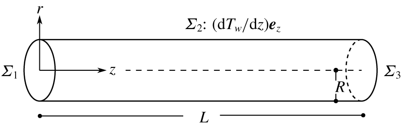
In order to implement the analytical framework which has been established in the previous section, a particular geometry is needed. A single regenerator channel is considered here, modelled as a cylinder of radius  $R$ and length
 $L$ as shown in figure 2. This shape is chosen based on the frequent use of honeycomb and stacked mesh screens in experiments. The cylinder models the tube-like structure and has better analytical properties than a square or hexagon. In practical terms, the circular shape avoids stress concentration and abrupt changes of heat transfer around the solid wall. As shown in figure 2, an axial temperature gradient
 $(\text{d}T_{w}/\text{d}z)\boldsymbol{e}_{z}$ is imposed on the curved surface
 $\unicode[STIX]{x1D6F4}_{2}$ which represents the wall.
Illustration of the cylindrical control volume considered in this work. The control surfaces are labelled  $\unicode[STIX]{x1D6F4}_{1}$ and
 $\unicode[STIX]{x1D6F4}_{3}$ for the two end surfaces and
 $\unicode[STIX]{x1D6F4}_{2}$ for the curved surface. The cylindrical coordinates are established at the centre of
 $\unicode[STIX]{x1D6F4}_{1}$. Surface
 $\unicode[STIX]{x1D6F4}_{2}$ represents the solid wall where heat transfer happens, and on the wall a temperature gradient in the axial direction is applied. Surface
 $\unicode[STIX]{x1D6F4}_{1}$ is referred to as the inlet and
 $\unicode[STIX]{x1D6F4}_{3}$ as the outlet.

To speed up the computation, two sets of assumptions are made to further simplify the problem: axisymmetric two-dimensional flow and Rott’s assumptions. The former is a reasonable assumption in cylindrical flow when the tangential change is negligible and the latter is a well-tested theory for thermoacoustic devices. Therefore the assumptions should involve minimal compromise for the physical understanding sought in this paper. Rott’s assumptions are reviewed in a subsequent section.
Finally, the solutions and numerical scheme are given. A global relative error was defined to test and ensure the accuracy of the numerical procedures and assumptions applied.
3.1 Axisymmetric two-dimensional flow assumption
The two-dimensional flow condition sets  $v_{\unicode[STIX]{x1D703}}=0$ and axisymmetry sets
 $\unicode[STIX]{x2202}f/\unicode[STIX]{x2202}\unicode[STIX]{x1D703}=0$, where
 $f$ is any scalar flow quantity or component of a vector. In cylindrical coordinates, the velocity gradient tensor reduces to
 $$\begin{eqnarray}\unicode[STIX]{x1D735}\boldsymbol{v}^{\prime }=\left[\begin{array}{@{}ccc@{}}{\displaystyle \frac{\unicode[STIX]{x2202}v_{r}^{\prime }}{\unicode[STIX]{x2202}r}} & 0 & {\displaystyle \frac{\unicode[STIX]{x2202}v_{z}^{\prime }}{\unicode[STIX]{x2202}r}}\\ 0 & {\displaystyle \frac{v_{r}^{\prime }}{r}} & 0\\ {\displaystyle \frac{\unicode[STIX]{x2202}v_{r}^{\prime }}{\unicode[STIX]{x2202}z}} & 0 & {\displaystyle \frac{\unicode[STIX]{x2202}v_{z}^{\prime }}{\unicode[STIX]{x2202}z}}\end{array}\right].\end{eqnarray}$$
Note that the gradient  $(\unicode[STIX]{x1D735}\boldsymbol{v}^{\prime })_{\unicode[STIX]{x1D703}\unicode[STIX]{x1D703}}$ is not zero because of the rotation of radial unit vector in
 $\boldsymbol{e}_{\unicode[STIX]{x1D703}}(1/r)(\unicode[STIX]{x2202}/\unicode[STIX]{x2202}\unicode[STIX]{x1D703})(v_{r}\boldsymbol{e}_{r})$, although
 $\unicode[STIX]{x2202}v_{r}/\unicode[STIX]{x2202}\unicode[STIX]{x1D703}=0$. Accordingly the viscous stress tensor, applying the Stokes hypothesis, is
 $$\begin{eqnarray}\displaystyle \unicode[STIX]{x1D749}^{\prime } & = & \displaystyle \unicode[STIX]{x1D707}(\unicode[STIX]{x1D735}\boldsymbol{v}^{\prime }+(\unicode[STIX]{x1D735}\boldsymbol{v}^{\prime })^{T})-\frac{2}{3}\unicode[STIX]{x1D707}(\unicode[STIX]{x1D735}\boldsymbol{\cdot }\boldsymbol{v}^{\prime })\unicode[STIX]{x1D644}\nonumber\\ \displaystyle & = & \displaystyle \unicode[STIX]{x1D707}\left[\begin{array}{@{}ccc@{}}{\displaystyle \frac{4}{3}}{\displaystyle \frac{\unicode[STIX]{x2202}v_{r}^{\prime }}{\unicode[STIX]{x2202}r}}-{\displaystyle \frac{2}{3}}{\displaystyle \frac{v_{r}^{\prime }}{r}}-{\displaystyle \frac{2}{3}}{\displaystyle \frac{\unicode[STIX]{x2202}v_{z}^{\prime }}{\unicode[STIX]{x2202}z}} & 0 & {\displaystyle \frac{\unicode[STIX]{x2202}v_{z}^{\prime }}{\unicode[STIX]{x2202}r}}+{\displaystyle \frac{\unicode[STIX]{x2202}v_{r}^{\prime }}{\unicode[STIX]{x2202}z}}\\ 0 & {\displaystyle \frac{4}{3}}{\displaystyle \frac{v_{r}^{\prime }}{r}}-{\displaystyle \frac{2}{3}}{\displaystyle \frac{\unicode[STIX]{x2202}v_{r}^{\prime }}{\unicode[STIX]{x2202}r}}-{\displaystyle \frac{2}{3}}{\displaystyle \frac{\unicode[STIX]{x2202}v_{z}^{\prime }}{\unicode[STIX]{x2202}z}} & 0\\ {\displaystyle \frac{\unicode[STIX]{x2202}v_{z}^{\prime }}{\unicode[STIX]{x2202}r}}+{\displaystyle \frac{\unicode[STIX]{x2202}v_{r}^{\prime }}{\unicode[STIX]{x2202}z}} & 0 & {\displaystyle \frac{4}{3}}{\displaystyle \frac{\unicode[STIX]{x2202}v_{z}^{\prime }}{\unicode[STIX]{x2202}z}}-{\displaystyle \frac{2}{3}}{\displaystyle \frac{1}{r}}{\displaystyle \frac{\unicode[STIX]{x2202}(rv_{r}^{\prime })}{\unicode[STIX]{x2202}r}}\end{array}\right].\qquad\end{eqnarray}$$
Hence the acoustic viscous dissipation function  ${\mathcal{D}}_{\unicode[STIX]{x1D708}}$ identified in (2.21) takes the reduced form of
 $$\begin{eqnarray}\displaystyle {\mathcal{D}}_{\unicode[STIX]{x1D708}} & = & \displaystyle \unicode[STIX]{x1D749}^{\prime }\boldsymbol{ : }\unicode[STIX]{x1D735}\boldsymbol{v}^{\prime }\nonumber\\ \displaystyle & = & \displaystyle 2\unicode[STIX]{x1D707}\left[\left({\displaystyle \frac{\unicode[STIX]{x2202}v_{r}^{\prime }}{\unicode[STIX]{x2202}r}}\right)^{2}+\left({\displaystyle \frac{v_{r}^{\prime }}{r}}\right)^{2}+\left({\displaystyle \frac{\unicode[STIX]{x2202}v_{z}^{\prime }}{\unicode[STIX]{x2202}z}}\right)^{2}+{\displaystyle \frac{1}{2}}\left({\displaystyle \frac{\unicode[STIX]{x2202}v_{z}^{\prime }}{\unicode[STIX]{x2202}r}}+{\displaystyle \frac{\unicode[STIX]{x2202}v_{r}^{\prime }}{\unicode[STIX]{x2202}z}}\right)^{2}-\frac{1}{3}\left({\displaystyle \frac{1}{r}}\frac{\unicode[STIX]{x2202}(rv_{r}^{\prime })}{\unicode[STIX]{x2202}r}+{\displaystyle \frac{\unicode[STIX]{x2202}v_{z}^{\prime }}{\unicode[STIX]{x2202}z}}\right)^{2}\right]\!.\nonumber\\ \displaystyle & & \displaystyle\end{eqnarray}$$
This concludes all the simplification obtained with the axisymmetric cylindrical assumption.
3.2 Rott’s assumptions
Rott (Reference Rott1969) proposed three key assumptions to further simplify the linearized governing equations (2.6)–(2.8). The first two assumptions can be mathematically summarized as
 $$\begin{eqnarray}\frac{\unicode[STIX]{x2202}p^{\prime }}{\unicode[STIX]{x2202}r}=0\end{eqnarray}$$
and
 $$\begin{eqnarray}\frac{\unicode[STIX]{x2202}T_{0}}{\unicode[STIX]{x2202}r}=0.\end{eqnarray}$$
The third one, ‘axial heat conduction in the acoustic wave and friction due to axial gradients are ignored’, is more subtle. The first part states that heat conduction happens in the radial direction only:
 $$\begin{eqnarray}q^{\prime }=k\unicode[STIX]{x1D735}T^{\prime }=k\frac{\unicode[STIX]{x2202}T^{\prime }}{\unicode[STIX]{x2202}r}\boldsymbol{e}_{r}.\end{eqnarray}$$
The second part states that the friction terms with  $\unicode[STIX]{x2202}/\unicode[STIX]{x2202}z$ are ignored, as indicated by the inclined cross line:

Despite its simplicity, Rott’s theory has proven to be in good agreement with experimental data when the linear approximation holds (see Backhaus & Swift Reference Backhaus and Swift2000; Wu et al. Reference Wu, Zhang, Dai and Luo2014). Therefore these underlying assumptions were used in the present study to simplify (2.6)–(2.8), yielding
 $$\begin{eqnarray}\displaystyle & \displaystyle \frac{\unicode[STIX]{x2202}\unicode[STIX]{x1D70C}^{\prime }}{\unicode[STIX]{x2202}t}+v_{z}^{\prime }\frac{\text{d}\unicode[STIX]{x1D70C}_{0}}{\text{d}z}+\unicode[STIX]{x1D70C}_{0}\frac{\unicode[STIX]{x2202}v_{z}^{\prime }}{\unicode[STIX]{x2202}z}+\unicode[STIX]{x1D70C}_{0}{\displaystyle \frac{1}{r}}\frac{\unicode[STIX]{x2202}(rv_{r}^{\prime })}{\unicode[STIX]{x2202}r}=0, & \displaystyle\end{eqnarray}$$
 $$\begin{eqnarray}\displaystyle & \displaystyle \unicode[STIX]{x1D70C}_{0}\frac{\unicode[STIX]{x2202}v_{z}^{\prime }}{\unicode[STIX]{x2202}t}=-\frac{\unicode[STIX]{x2202}p^{\prime }}{\unicode[STIX]{x2202}z}+\unicode[STIX]{x1D707}\frac{\unicode[STIX]{x2202}^{2}v_{z}^{\prime }}{\unicode[STIX]{x2202}r^{2}}+\unicode[STIX]{x1D707}{\displaystyle \frac{1}{r}}{\displaystyle \frac{\unicode[STIX]{x2202}v_{z}^{\prime }}{\unicode[STIX]{x2202}r}}, & \displaystyle\end{eqnarray}$$
 $$\begin{eqnarray}\displaystyle & \displaystyle \unicode[STIX]{x1D70C}_{0}T_{0}\frac{\unicode[STIX]{x2202}s^{\prime }}{\unicode[STIX]{x2202}t}+\unicode[STIX]{x1D70C}_{0}T_{0}v_{z}^{\prime }\frac{\text{d}s_{0}}{\text{d}z}=k\frac{\unicode[STIX]{x2202}^{2}T^{\prime }}{\unicode[STIX]{x2202}r^{2}}+k{\displaystyle \frac{1}{r}}\frac{\unicode[STIX]{x2202}T^{\prime }}{\unicode[STIX]{x2202}r}, & \displaystyle\end{eqnarray}$$
which in this study are subject to the following boundary conditions:
 $$\begin{eqnarray}T_{0}(R,z)=T_{w}(z),\quad T^{\prime }(R,z)=0,\quad \boldsymbol{v}^{\prime }(R,z)=0,\quad v_{r}^{\prime }(0,z)=0,\quad \forall z\in [0,L],\end{eqnarray}$$
where function  $T_{w}(z)$ is given. The momentum equation in the radial direction is reduced to
 $\unicode[STIX]{x2202}p^{\prime }/\unicode[STIX]{x2202}r=0$ and mean temperature
 $$\begin{eqnarray}T_{0}(r,z)=T_{w}(z).\end{eqnarray}$$
This concludes the simplification obtained with Rott’s assumptions.
3.3 Dimensional analysis
To further simplify the disturbance energy equation (2.27) and reduce the number of independent parameters, the problem is non-dimensionalized. Scaling procedures follow the ones used by In’t Panhuis et al. (Reference In’t Panhuis, Rienstra, Molenaar and Slot2009). The dimensionless variables, denoted by an asterisk, are
 $$\begin{eqnarray}\left.\begin{array}{@{}c@{}}\displaystyle r=Rr^{\ast },\quad z=Lz^{\ast },\quad t=\frac{1}{\unicode[STIX]{x1D714}}t^{\ast },\quad v_{z}^{\prime }=c_{ref}v_{z}^{\prime \ast },\quad v_{r}^{\prime }=\unicode[STIX]{x1D700}c_{ref}v_{r}^{\prime \ast },\\ \displaystyle \unicode[STIX]{x1D70C}^{\prime }=\unicode[STIX]{x1D70C}_{ref}\unicode[STIX]{x1D70C}^{\prime \ast },\quad \unicode[STIX]{x1D70C}_{0}=\unicode[STIX]{x1D70C}_{ref}\unicode[STIX]{x1D70C}_{0}^{\ast },\quad p^{\prime }=\unicode[STIX]{x1D70C}_{ref}c_{ref}^{2}p^{\prime \ast },\quad p_{0}=\unicode[STIX]{x1D70C}_{ref}c_{ref}^{2}p_{0}^{\ast },\quad T^{\prime }=\frac{c_{ref}^{2}}{c_{p}}T^{\prime \ast },\\ \displaystyle T_{0}=\frac{c_{ref}^{2}}{c_{p}}T_{0}^{\ast },\quad s=c_{p}s^{\prime \ast },\quad s_{0}=c_{p}s_{0}^{\ast },\quad \unicode[STIX]{x1D707}=\unicode[STIX]{x1D707}_{ref}\unicode[STIX]{x1D707}^{\ast },\quad k=k_{ref}k^{\ast },\end{array}\right\}\end{eqnarray}$$
where  $\unicode[STIX]{x1D700}=R/L$ is the aspect ratio and the reference point for
 $\unicode[STIX]{x1D70C}_{ref}$,
 $c_{ref}$,
 $\unicode[STIX]{x1D707}_{ref}$ and
 $k_{ref}$ was set at the mid-point (
 $z_{ref}=L/2$) of the regenerator. The governing equations in dimensionless form are
 $$\begin{eqnarray}\displaystyle & \displaystyle He\frac{\unicode[STIX]{x2202}\unicode[STIX]{x1D70C}^{\prime \ast }}{\unicode[STIX]{x2202}t^{\ast }}+v_{z}^{\prime \ast }\frac{\text{d}\unicode[STIX]{x1D70C}_{0}^{\ast }}{\text{d}z^{\ast }}+\unicode[STIX]{x1D70C}_{0}^{\ast }\frac{\unicode[STIX]{x2202}v_{z}^{\prime \ast }}{\unicode[STIX]{x2202}z^{\ast }}+\unicode[STIX]{x1D70C}_{0}^{\ast }\frac{1}{r^{\ast }}\frac{\unicode[STIX]{x2202}(r^{\ast }v_{r}^{\prime \ast })}{\unicode[STIX]{x2202}r^{\ast }}=0, & \displaystyle\end{eqnarray}$$
 $$\begin{eqnarray}\displaystyle & \displaystyle \unicode[STIX]{x1D70C}_{0}^{\ast }\frac{\unicode[STIX]{x2202}v_{z}^{\prime \ast }}{\unicode[STIX]{x2202}t^{\ast }}=-\frac{1}{He}\frac{\unicode[STIX]{x2202}p^{\prime \ast }}{\unicode[STIX]{x2202}z^{\ast }}+\frac{1}{Wo^{2}}\unicode[STIX]{x1D707}^{\ast }\left(\frac{\unicode[STIX]{x2202}^{2}v_{z}^{\prime \ast }}{\unicode[STIX]{x2202}r^{\ast 2}}+\frac{1}{r^{\ast }}\frac{\unicode[STIX]{x2202}v_{z}^{\prime \ast }}{\unicode[STIX]{x2202}r^{\ast }}\right), & \displaystyle\end{eqnarray}$$
 $$\begin{eqnarray}\displaystyle & \displaystyle \unicode[STIX]{x1D70C}_{0}^{\ast }T_{0}^{\ast }\frac{\unicode[STIX]{x2202}s^{\prime \ast }}{\unicode[STIX]{x2202}t^{\ast }}+\frac{1}{He}\unicode[STIX]{x1D70C}_{0}^{\ast }T_{0}^{\ast }v_{z}^{\prime \ast }\frac{\text{d}s_{0}^{\ast }}{\text{d}z^{\ast }}=\frac{1}{Pr\cdot Wo^{2}}\frac{k\unicode[STIX]{x1D714}}{p_{0}}\left(\frac{\unicode[STIX]{x2202}^{2}T^{\prime \ast }}{\unicode[STIX]{x2202}r^{\ast 2}}+\frac{1}{r^{\ast }}\frac{\unicode[STIX]{x2202}T^{\prime \ast }}{\unicode[STIX]{x2202}r^{\ast }}\right), & \displaystyle\end{eqnarray}$$
where
 $$\begin{eqnarray}He=\frac{\unicode[STIX]{x1D714}L}{c_{ref}},\quad Wo=R\left(\frac{\unicode[STIX]{x1D714}\unicode[STIX]{x1D70C}_{ref}}{\unicode[STIX]{x1D707}_{ref}}\right)^{1/2}\end{eqnarray}$$
are the Helmholtz number and the Womersley number, respectively, with  $Pr$ being the Prandtl number.
Parameter  $Wo^{2}$ is the ratio of transient inertial force (
 $\unicode[STIX]{x1D70C}_{ref}(c_{ref}/(1/\unicode[STIX]{x1D714}))$) to viscous force (
 $\unicode[STIX]{x1D707}_{ref}(c_{ref}/R)(1/R)$). In fact
 $Wo^{2}$ is also the Reynolds number when the length and time scales, instead of velocity scale, are imposed (which leads to the Strouhal number
 $St=1$), namely
 $$\begin{eqnarray}Wo^{2}=Re=\frac{\unicode[STIX]{x1D70C}_{ref}(\unicode[STIX]{x1D714}R)R}{\unicode[STIX]{x1D707}_{ref}}.\end{eqnarray}$$
Correspondingly,  $Pr\cdot Wo^{2}$ would be the Péclet number, i.e.
 $$\begin{eqnarray}Pr\cdot Wo^{2}=\frac{c_{p}\unicode[STIX]{x1D707}_{ref}}{k_{ref}}\frac{\unicode[STIX]{x1D70C}_{ref}(\unicode[STIX]{x1D714}R)R}{\unicode[STIX]{x1D707}_{ref}}=Pe.\end{eqnarray}$$
Some authors (e.g. Worlikar & Knio Reference Worlikar and Knio1996) prefer the notion of  $Re$ and
 $Pe$, but in this paper
 $Wo^{2}$ is used because its physical meaning can be interpreted in various ways. Firstly,
 $Wo^{2}$ and
 $Pr\cdot Wo^{2}$ can be interpreted as the ratio of two distances:
 $$\begin{eqnarray}Wo=\sqrt{2}\frac{R}{\unicode[STIX]{x1D6FF}_{\unicode[STIX]{x1D708}}},\quad \sqrt{Pr}\cdot Wo=\sqrt{2}\frac{R}{\unicode[STIX]{x1D6FF}_{k}},\end{eqnarray}$$
where
 $$\begin{eqnarray}\unicode[STIX]{x1D6FF}_{\unicode[STIX]{x1D708}}=\sqrt{\frac{2\unicode[STIX]{x1D707}}{\unicode[STIX]{x1D714}\unicode[STIX]{x1D70C}_{0}}},\quad \unicode[STIX]{x1D6FF}_{k}=\sqrt{\frac{2k}{\unicode[STIX]{x1D714}\unicode[STIX]{x1D70C}_{0}c_{p}}}\end{eqnarray}$$
are the depth of the Stokes layer and its thermal counterpart, respectively. They are the characteristic length of momentum and thermal diffusion in one period. Therefore if  $Wo\sim O(1)$ the whole channel is filled with oscillatory boundary layer as in the case of regenerators considered here, and
 $Wo\gg 1$ is found in ordinary acoustic resonators.
Another interpretation of  $Wo^{2}$ is proposed by Tominaga (Reference Tominaga1995), as the ratio of two time scales:
 $$\begin{eqnarray}Wo^{2}=\unicode[STIX]{x1D714}t_{\unicode[STIX]{x1D708}},\quad Pr\cdot Wo^{2}=\unicode[STIX]{x1D714}t_{k},\end{eqnarray}$$
and
 $$\begin{eqnarray}t_{\unicode[STIX]{x1D708}}=\frac{R^{2}}{\unicode[STIX]{x1D708}},\quad t_{k}=\frac{R^{2}}{\unicode[STIX]{x1D6FC}},\end{eqnarray}$$
where  $\unicode[STIX]{x1D708}$ is the kinematic viscosity and
 $\unicode[STIX]{x1D6FC}$ the thermal diffusivity, while
 $t_{\unicode[STIX]{x1D708}}$ and
 $t_{k}$ characterize the time of momentum and thermal diffusion across the channel area. Therefore
 $Wo^{2}$ is the time scale of diffusion measured in the period of oscillation.
3.3.1 Simplification of disturbance energy terms
In the following, the scales obtained from dimensional analysis are used to achieve the simplification of disturbance energy terms. First consider the velocity gradients:
 $$\begin{eqnarray}\left.\begin{array}{@{}cccccc@{}} & {\displaystyle \frac{\unicode[STIX]{x2202}v_{r}^{\prime }}{\unicode[STIX]{x2202}z}} & {\displaystyle \frac{\unicode[STIX]{x2202}v_{r}^{\prime }}{\unicode[STIX]{x2202}r}} & {\displaystyle \frac{v_{r}^{\prime }}{r}} & {\displaystyle \frac{\unicode[STIX]{x2202}v_{z}^{\prime }}{\unicode[STIX]{x2202}z}} & {\displaystyle \frac{\unicode[STIX]{x2202}v_{z}^{\prime }}{\unicode[STIX]{x2202}r}}\\ {\displaystyle \frac{c_{ref}}{L}}\cdot & \bigg(\unicode[STIX]{x1D700} & 1 & 1 & 1 & {\displaystyle \frac{1}{\unicode[STIX]{x1D700}}}\bigg).\end{array}\right\}\end{eqnarray}$$
The scales are written beneath as the product of a common factor (in this case  $c_{ref}/L$) and relative orders defined as
 $\unicode[STIX]{x1D700}^{2}$,
 $\unicode[STIX]{x1D700}$, 1,
 $1/\unicode[STIX]{x1D700}$,
 $1/\unicode[STIX]{x1D700}^{2}$. Note that the aspect ratio
 $\unicode[STIX]{x1D700}$ is small,
 $\unicode[STIX]{x1D700}\sim O(0.01)$.
The rationale behind Rott’s third assumption, namely (3.6) and (3.7), becomes clearer with this dimensional analysis, because
 $$\begin{eqnarray}\left.\begin{array}{@{}l@{}}(\unicode[STIX]{x1D735}\boldsymbol{\cdot }\unicode[STIX]{x1D749}^{\prime })\boldsymbol{\cdot }\boldsymbol{e}_{z}=\unicode[STIX]{x1D707}\left[{\displaystyle \frac{\unicode[STIX]{x2202}^{2}v_{z}^{\prime }}{\unicode[STIX]{x2202}r^{2}}}+{\displaystyle \frac{\unicode[STIX]{x2202}^{2}v_{r}^{\prime }}{\unicode[STIX]{x2202}r\unicode[STIX]{x2202}z}}+{\displaystyle \frac{1}{r}}{\displaystyle \frac{\unicode[STIX]{x2202}v_{z}^{\prime }}{\unicode[STIX]{x2202}r}}+{\displaystyle \frac{1}{r}}{\displaystyle \frac{\unicode[STIX]{x2202}v_{r}^{\prime }}{\unicode[STIX]{x2202}z}}+{\displaystyle \frac{1}{\unicode[STIX]{x2202}z}}\left({\displaystyle \frac{4}{3}}{\displaystyle \frac{\unicode[STIX]{x2202}v_{z}^{\prime }}{\unicode[STIX]{x2202}z}}-{\displaystyle \frac{2}{3}}{\displaystyle \frac{1}{r}}{\displaystyle \frac{\unicode[STIX]{x2202}(rv_{r}^{\prime })}{\unicode[STIX]{x2202}r}}\right)\right]\!\\ \hspace{18.0pt}{\displaystyle \frac{\unicode[STIX]{x1D707}_{ref}c_{ref}}{L^{2}}}\cdot \hspace{15.60004pt}\left({\displaystyle \frac{1}{\unicode[STIX]{x1D700}^{2}}}\hspace{24.0pt}1\hspace{26.39996pt}{\displaystyle \frac{1}{\unicode[STIX]{x1D700}^{2}}}\hspace{28.79993pt}1\hspace{92.39996pt}1\hspace{40.79993pt}\right).\end{array}\right\}\end{eqnarray}$$
The leading terms  $\unicode[STIX]{x2202}^{2}v_{z}^{\prime }/\unicode[STIX]{x2202}r^{2}$ and
 $(1/r)(\unicode[STIX]{x2202}v_{z}^{\prime }/\unicode[STIX]{x2202}r)$, which are kept in the assumption, are two orders of magnitude larger than the rest. Similarly,
 $$\begin{eqnarray}\left.\begin{array}{@{}l@{}}\hspace{18.0pt}\boldsymbol{q}^{\prime }=k\left({\displaystyle \frac{\unicode[STIX]{x2202}T^{\prime }}{\unicode[STIX]{x2202}r}}\boldsymbol{e}_{r}+{\displaystyle \frac{\unicode[STIX]{x2202}T^{\prime }}{\unicode[STIX]{x2202}z}}\boldsymbol{e}_{z}\right)\!\\ {\displaystyle \frac{k_{ref}T_{ref}}{L}}\cdot \hspace{6.0pt}\left(~{\displaystyle \frac{1}{\unicode[STIX]{x1D700}}}\hspace{48.0pt}1\right).\end{array}\right\}\end{eqnarray}$$
The radial heat flux is one order of magnitude larger than the axial heat flux.
Now one applies the order-of-magnitude analysis to the terms in the disturbance energy equation. The scales of squared terms in viscous dissipation are
 $$\begin{eqnarray}\left.\begin{array}{@{}l@{}}\hspace{42.0pt}\left({\displaystyle \frac{\unicode[STIX]{x2202}v_{r}^{\prime }}{\unicode[STIX]{x2202}r}}\right)^{2}+\left({\displaystyle \frac{v_{r}^{\prime }}{r}}\right)^{2}+\left({\displaystyle \frac{\unicode[STIX]{x2202}v_{z}^{\prime }}{\unicode[STIX]{x2202}z}}\right)^{2}+{\displaystyle \frac{1}{2}}\left({\displaystyle \frac{\unicode[STIX]{x2202}v_{z}^{\prime }}{\unicode[STIX]{x2202}r}}+{\displaystyle \frac{\unicode[STIX]{x2202}v_{r}^{\prime }}{\unicode[STIX]{x2202}z}}\right)^{2}-{\displaystyle \frac{1}{3}}\left({\displaystyle \frac{1}{r}}{\displaystyle \frac{\unicode[STIX]{x2202}(rv_{r}^{\prime })}{\unicode[STIX]{x2202}r}}+{\displaystyle \frac{\unicode[STIX]{x2202}v_{z}^{\prime }}{\unicode[STIX]{x2202}z}}\right)^{2}\\ \left({\displaystyle \frac{c_{ref}}{L}}\right)^{2}\cdot \hspace{6.0pt}\left(1\hspace{42.0pt}1\hspace{42.0pt}1\hspace{48.0pt}{\displaystyle \frac{1}{\unicode[STIX]{x1D700}^{2}}}\hspace{20.39996pt}\unicode[STIX]{x1D700}^{2}\hspace{66.0pt}1\hspace{30.0pt}1\right).\end{array}\right\}\end{eqnarray}$$
The leading term  $(\unicode[STIX]{x2202}v_{z}^{\prime }/\unicode[STIX]{x2202}r)^{2}$ is two orders of magnitude larger than the rest, so the viscous dissipation can be assumed to be
 $$\begin{eqnarray}{\mathcal{D}}_{\unicode[STIX]{x1D708}}=\unicode[STIX]{x1D707}\left({\displaystyle \frac{\unicode[STIX]{x2202}v_{z}^{\prime }}{\unicode[STIX]{x2202}r}}\right)^{2},\end{eqnarray}$$
without losing much accuracy.
For thermal dissipation, simply applying Rott’s assumption equation (3.6) yields
 $$\begin{eqnarray}{\mathcal{D}}_{k}=k\frac{\left(\unicode[STIX]{x1D735}T^{\prime }\right)^{2}}{T_{0}}=\frac{k}{T_{0}}\left(\frac{\unicode[STIX]{x2202}T^{\prime }}{\unicode[STIX]{x2202}r}\right)^{2}.\end{eqnarray}$$
For the production term, given that the direction of  $\unicode[STIX]{x1D735}T_{0}$ as shown in figure 2 is orthogonal to the direction of simplified heat flux, it takes the form
 $$\begin{eqnarray}\displaystyle {\mathcal{P}} & = & \displaystyle \left(k\frac{T^{\prime }}{T_{0}}\unicode[STIX]{x1D735}T^{\prime }-T_{0}\unicode[STIX]{x1D70C}_{0}s^{\prime }\boldsymbol{v}^{\prime }\right)\boldsymbol{\cdot }\frac{\unicode[STIX]{x1D735}T_{0}}{T_{0}}\nonumber\\ \displaystyle & = & \displaystyle k\frac{T^{\prime }}{T_{0}^{2}}\frac{\unicode[STIX]{x2202}T^{\prime }}{\unicode[STIX]{x2202}r}\boldsymbol{e}_{r}\frac{\text{d}T_{0}}{\text{d}z}\boldsymbol{e}_{z}-\unicode[STIX]{x1D70C}_{0}s^{\prime }v_{z}^{\prime }\boldsymbol{e}_{z}\frac{\text{d}T_{0}}{\text{d}z}\boldsymbol{e}_{z}-\unicode[STIX]{x1D70C}_{0}s^{\prime }v_{r}^{\prime }\boldsymbol{e}_{r}\frac{\text{d}T_{0}}{\text{d}z}\boldsymbol{e}_{z}\nonumber\\ \displaystyle & = & \displaystyle -\unicode[STIX]{x1D70C}_{0}s^{\prime }v_{z}^{\prime }\frac{\text{d}T_{0}}{\text{d}z}.\end{eqnarray}$$
Finally, one considers the disturbance energy flux term by term:
 $$\begin{eqnarray}\unicode[STIX]{x1D735}\boldsymbol{\cdot }I=\unicode[STIX]{x1D735}\boldsymbol{\cdot }(p^{\prime }\boldsymbol{v}^{\prime })-\unicode[STIX]{x1D735}\boldsymbol{\cdot }(\unicode[STIX]{x1D749}^{\prime }\boldsymbol{\cdot }\boldsymbol{v}^{\prime })-\unicode[STIX]{x1D735}\boldsymbol{\cdot }\left(\frac{T^{\prime }}{T_{0}}k\unicode[STIX]{x1D735}T^{\prime }\right).\end{eqnarray}$$
With  $\unicode[STIX]{x1D749}^{\prime }:\unicode[STIX]{x1D735}\boldsymbol{v}^{\prime }$ and
 $\boldsymbol{v}^{\prime }\boldsymbol{\cdot }(\unicode[STIX]{x1D735}\boldsymbol{\cdot }\unicode[STIX]{x1D749}^{\prime })$ already individually simplified, given the divergence identity, it must satisfy
 $$\begin{eqnarray}\displaystyle \unicode[STIX]{x1D735}\boldsymbol{\cdot }(\unicode[STIX]{x1D749}^{\prime }\boldsymbol{\cdot }\boldsymbol{v}^{\prime }) & = & \displaystyle \boldsymbol{v}^{\prime }\boldsymbol{\cdot }(\unicode[STIX]{x1D735}\boldsymbol{\cdot }\unicode[STIX]{x1D749}^{\prime })+\unicode[STIX]{x1D749}^{\prime }\boldsymbol{ : }\unicode[STIX]{x1D735}\boldsymbol{v}^{\prime }\nonumber\\ \displaystyle & = & \displaystyle \unicode[STIX]{x1D707}\left[v_{z}\frac{\unicode[STIX]{x2202}^{2}v_{z}}{\unicode[STIX]{x2202}r^{2}}+v_{z}{\displaystyle \frac{1}{r}}{\displaystyle \frac{\unicode[STIX]{x2202}v_{z}^{\prime }}{\unicode[STIX]{x2202}r}}+\left({\displaystyle \frac{\unicode[STIX]{x2202}v_{z}^{\prime }}{\unicode[STIX]{x2202}r}}\right)^{2}\right].\end{eqnarray}$$
From the simplified form of  $\unicode[STIX]{x1D735}\boldsymbol{\cdot }(\unicode[STIX]{x1D749}^{\prime }\boldsymbol{\cdot }\boldsymbol{v}^{\prime })$,
 $\unicode[STIX]{x1D749}^{\prime }\boldsymbol{ : }\unicode[STIX]{x1D735}\boldsymbol{v}^{\prime }$ and
 $\boldsymbol{v}^{\prime }\boldsymbol{\cdot }(\unicode[STIX]{x1D735}\boldsymbol{\cdot }\unicode[STIX]{x1D749}^{\prime })$, an equivalent stress tensor can be defined as
 $$\begin{eqnarray}\unicode[STIX]{x1D749}_{e}^{\prime }=\left[\begin{array}{@{}ccc@{}}0 & 0 & \unicode[STIX]{x1D70F}_{rz}\\ 0 & 0 & 0\\ 0 & 0 & 0\end{array}\right]=\unicode[STIX]{x1D707}\left[\begin{array}{@{}ccc@{}}0 & 0 & {\displaystyle \frac{\unicode[STIX]{x2202}v_{z}^{\prime }}{\unicode[STIX]{x2202}r}}\\ 0 & 0 & 0\\ 0 & 0 & 0\end{array}\right].\end{eqnarray}$$
Note that the stress tensor is said to be ‘equivalent’ because it leads to the correct simplified form (3.7), (3.28), (3.32) but it does not obey symmetry and the Stokes hypothesis. The equivalent tensor is useful in determining  $\unicode[STIX]{x1D749}^{\prime }\boldsymbol{\cdot }\boldsymbol{v}^{\prime }$ in the following paragraphs.
Similarly,
 $$\begin{eqnarray}\displaystyle \unicode[STIX]{x1D735}\boldsymbol{\cdot }\left(\frac{T^{\prime }}{T_{0}}k\unicode[STIX]{x1D735}T^{\prime }\right) & = & \displaystyle \frac{T^{\prime }}{T_{0}}k\unicode[STIX]{x1D6FB}^{2}T^{\prime }+k\frac{(\unicode[STIX]{x1D735}T^{\prime })^{2}}{T_{0}}-k\frac{T^{\prime }}{T_{0}^{2}}\unicode[STIX]{x1D735}T_{0}\boldsymbol{\cdot }\unicode[STIX]{x1D735}T^{\prime }\nonumber\\ \displaystyle & = & \displaystyle \frac{T^{\prime }}{T_{0}}k\left(\frac{\unicode[STIX]{x2202}^{2}T^{\prime }}{\unicode[STIX]{x2202}r^{2}}+{\displaystyle \frac{1}{r}}\frac{\unicode[STIX]{x2202}T^{\prime }}{\unicode[STIX]{x2202}r}\right)+\frac{1}{T_{0}}k\left(\frac{\unicode[STIX]{x2202}T^{\prime }}{\unicode[STIX]{x2202}r}\right)^{2}.\end{eqnarray}$$
Taking advantage of the boundary conditions,  $\unicode[STIX]{x1D735}\boldsymbol{\cdot }I$ can be further simplified in the integral form. The control volume in this study was a cylinder bounded by three surfaces
 $\unicode[STIX]{x1D6F4}_{1}$,
 $\unicode[STIX]{x1D6F4}_{2}$ and
 $\unicode[STIX]{x1D6F4}_{3}$ as shown in figure 2. Integrating the time-averaged disturbance energy balance relation (2.27) over the control volume and applying Green’s theorem yields
 $$\begin{eqnarray}\iint _{\unicode[STIX]{x1D6F4}}\boldsymbol{n}\boldsymbol{\cdot }\overline{I}\,\text{d}S=-\iiint _{\unicode[STIX]{x1D6FA}}\overline{{\mathcal{D}}_{\unicode[STIX]{x1D708}}}\,\text{d}V-\iiint _{\unicode[STIX]{x1D6FA}}\overline{{\mathcal{D}}_{k}}\,\text{d}V+\iiint _{\unicode[STIX]{x1D6FA}}\overline{{\mathcal{P}}}\,\text{d}V,\end{eqnarray}$$
where  $\boldsymbol{n}$ is the outward-pointing unit normal vector on
 $\unicode[STIX]{x1D6F4}$. Equation (3.35) is the integral form of the time-averaged disturbance energy balance relation.
The instantaneous disturbance energy flux is
 $$\begin{eqnarray}\iint _{\unicode[STIX]{x1D6F4}}\boldsymbol{n}\boldsymbol{\cdot }I\,\text{d}S=\iint _{\unicode[STIX]{x1D6F4}}\boldsymbol{n}\boldsymbol{\cdot }\left(p^{\prime }\boldsymbol{v}^{\prime }-\unicode[STIX]{x1D749}^{\prime }\boldsymbol{\cdot }\boldsymbol{v}^{\prime }-\frac{T^{\prime }}{T_{0}}k\unicode[STIX]{x1D735}T^{\prime }\right)\,\text{d}S.\end{eqnarray}$$
On  $\unicode[STIX]{x1D6F4}_{2}$, the boundary conditions (3.11) set the integration (3.36) to zero and on
 $\unicode[STIX]{x1D6F4}_{1}$ and
 $\unicode[STIX]{x1D6F4}_{3}$,
 $\boldsymbol{n}$ was parallel to
 $\boldsymbol{e}_{z}$, so (3.36) becomes
 $$\begin{eqnarray}\displaystyle \iint _{\unicode[STIX]{x1D6F4}}\boldsymbol{n}\boldsymbol{\cdot }I\,\text{d}S & = & \displaystyle \iint _{\unicode[STIX]{x1D6F4}_{3}}\boldsymbol{e}_{z}\boldsymbol{\cdot }\left(p^{\prime }\boldsymbol{v}^{\prime }-\unicode[STIX]{x1D749}^{\prime }\boldsymbol{\cdot }\boldsymbol{v}^{\prime }-\frac{T^{\prime }}{T_{0}}k\unicode[STIX]{x1D735}T^{\prime }\right)\,\text{d}S\nonumber\\ \displaystyle & & \displaystyle -\iint _{\unicode[STIX]{x1D6F4}_{1}}\boldsymbol{e}_{z}\boldsymbol{\cdot }\left(p^{\prime }\boldsymbol{v}^{\prime }-\unicode[STIX]{x1D749}^{\prime }\boldsymbol{\cdot }\boldsymbol{v}^{\prime }-\frac{T^{\prime }}{T_{0}}k\unicode[STIX]{x1D735}T^{\prime }\right)\,\text{d}S.\end{eqnarray}$$
With the equivalent stress tensor already defined, it is found that
 $$\begin{eqnarray}\displaystyle & \displaystyle \unicode[STIX]{x1D749}^{\prime }\boldsymbol{\cdot }\boldsymbol{v}^{\prime }=\unicode[STIX]{x1D749}_{e}^{\prime }\boldsymbol{\cdot }\boldsymbol{v}^{\prime }=\unicode[STIX]{x1D70F}_{rz}^{\prime }v_{z}^{\prime }\boldsymbol{e}_{r}=\unicode[STIX]{x1D707}{\displaystyle \frac{\unicode[STIX]{x2202}v_{z}^{\prime }}{\unicode[STIX]{x2202}r}}v_{z}^{\prime }\boldsymbol{e}_{r}, & \displaystyle\end{eqnarray}$$
 $$\begin{eqnarray}\displaystyle & \displaystyle \frac{T^{\prime }}{T_{0}}k\unicode[STIX]{x1D735}T^{\prime }=\frac{T^{\prime }}{T_{0}}k\frac{\unicode[STIX]{x2202}T^{\prime }}{\unicode[STIX]{x2202}r}\boldsymbol{e}_{r}, & \displaystyle\end{eqnarray}$$
which are both orthogonal to  $\boldsymbol{e}_{z}$.
Hence the final simplified expression of  $\iint _{\unicode[STIX]{x1D6F4}}\boldsymbol{n}\boldsymbol{\cdot }I\,\text{d}S$ in a cylindrical domain is
 $$\begin{eqnarray}\iint _{\unicode[STIX]{x1D6F4}}\boldsymbol{n}\boldsymbol{\cdot }I\,\text{d}S=\iint _{\unicode[STIX]{x1D6F4}_{3}}p^{\prime }v_{z}^{\prime }\,\text{d}S-\iint _{\unicode[STIX]{x1D6F4}_{1}}p^{\prime }v_{z}^{\prime }\,\text{d}S.\end{eqnarray}$$
Therefore it is shown that, after the simplification, the disturbance energy flux in a cylindrical domain reduces to the classic acoustic flux.
This section has reported in detail the simplification of  ${\mathcal{D}}_{\unicode[STIX]{x1D708}}$,
 ${\mathcal{D}}_{k}$,
 ${\mathcal{P}}$ and
 $\iint \boldsymbol{n}\boldsymbol{\cdot }I\,\text{d}S$, taking the form of (3.28), (3.29), (3.30) and (3.40), respectively.
3.3.2 Dimensionless disturbance energy balance
The integral form of the disturbance energy balance is non-dimensionalized using integrated inlet disturbance energy flux  $(\boldsymbol{n}\boldsymbol{\cdot }\overline{I})_{\unicode[STIX]{x1D6F4}_{1}}$. Shorthand notations
 $(\cdot )_{cv}$ and
 $(\cdot )_{cs}$ are used for
 $\iiint _{\unicode[STIX]{x1D6FA}}\cdot \text{d}V$ and
 $\iint _{\unicode[STIX]{x1D6F4}}\cdot \text{d}S$, respectively. The equation takes the form
 $$\begin{eqnarray}(\boldsymbol{n}\boldsymbol{\cdot }\overline{I})_{cs}^{\ast }=-(\overline{{\mathcal{D}}_{\unicode[STIX]{x1D708}}})_{cv}^{\ast }-(\overline{{\mathcal{D}}_{k}})_{cv}^{\ast }+(\overline{{\mathcal{P}}})_{cv}^{\ast },\end{eqnarray}$$
where each term
 $$\begin{eqnarray}(\cdot )_{cs|cv}^{\ast }=\frac{(\cdot )_{cs|cv}}{(\boldsymbol{n}\boldsymbol{\cdot }\overline{I})_{\unicode[STIX]{x1D6F4}_{1}}}.\end{eqnarray}$$
The term  $(\boldsymbol{n}\boldsymbol{\cdot }\overline{I})_{cs}^{\ast }$ then represents the relative wave growth;
 $(\overline{{\mathcal{P}}})^{\ast }$,
 $(\overline{{\mathcal{D}}_{\unicode[STIX]{x1D708}}})^{\ast }$ and
 $(\overline{{\mathcal{D}}_{k}})^{\ast }$ are production, viscous dissipation and thermal dissipation relative to the energy transported by the wave, respectively. The benefit of scaling in this way is to offer better intuition since terms are expressed as fractions or multiples of inlet energy and are hence
 $O(1)$. Also the equality of left- and right-hand sides of the equation can be easily shown by taking the difference
 $\unicode[STIX]{x1D6E5}^{\ast }=(\overline{{\mathcal{P}}})_{cv}^{\ast }-(\overline{{\mathcal{D}}_{\unicode[STIX]{x1D708}}})_{cv}^{\ast }-(\overline{{\mathcal{D}}_{\unicode[STIX]{x1D708}}})_{cv}^{\ast }-(\boldsymbol{n}\boldsymbol{\cdot }\overline{I})_{cs}^{\ast }$.
It is worth noting that another possible scaling procedures is to non-dimensionalize the energy terms by the respective flow variables. For example,
 $$\begin{eqnarray}(\overline{{\mathcal{D}}_{k}})_{cv}=\int _{0}^{L}\int _{0}^{R}\frac{k}{T_{0}}\left(\frac{\unicode[STIX]{x2202}T^{\prime }}{\unicode[STIX]{x2202}r}\right)^{2}r\,\text{d}r\,\text{d}l=k_{ref}T_{ref}L\int _{0}^{1}\int _{0}^{1}\frac{k^{\ast }}{T_{0}^{\ast }}\left(\frac{\unicode[STIX]{x2202}T^{\prime \ast }}{\unicode[STIX]{x2202}r^{\ast }}\right)^{2}r^{\ast }\,\text{d}r^{\ast }\,\text{d}l^{\ast }.\end{eqnarray}$$
Define
 $$\begin{eqnarray}(\overline{{\mathcal{D}}_{k}})^{\dagger }=\frac{k^{\ast }}{T_{0}^{\ast }}\left(\frac{\unicode[STIX]{x2202}T^{\prime \ast }}{\unicode[STIX]{x2202}r^{\ast }}\right)^{2},\quad (\overline{{\mathcal{D}}_{k}})_{cv}^{\dagger }=\int _{0}^{1}\int _{0}^{1}(\overline{{\mathcal{D}}_{k}})^{\dagger }r^{\ast }\,\text{d}r^{\ast }\,\text{d}l^{\ast },\end{eqnarray}$$
where the dagger ( $\dagger$) superscript denotes non-dimensionalization using corresponding flow variables. It can be shown that the two non-dimensionalization methods are equivalent, because
 $$\begin{eqnarray}(\overline{{\mathcal{D}}_{k}})_{cv}^{\ast }=\frac{(\overline{{\mathcal{D}}_{k}})_{cv}}{(\boldsymbol{n}\boldsymbol{\cdot }\overline{I})_{\unicode[STIX]{x1D6F4}_{1}}}=\frac{k_{ref}{\displaystyle \frac{c_{ref}^{2}}{c_{p}}}L(\overline{{\mathcal{D}}_{k}})^{\dagger }}{\unicode[STIX]{x1D70C}_{ref}c_{ref}^{3}R^{2}(\boldsymbol{n}\boldsymbol{\cdot }\overline{I})_{\unicode[STIX]{x1D6F4}_{1}}^{\dagger }}=\frac{He}{Wo^{2}}\frac{(\overline{{\mathcal{D}}_{k}})^{\dagger }}{(\boldsymbol{n}\boldsymbol{\cdot }\overline{I})_{\unicode[STIX]{x1D6F4}_{1}}^{\dagger }}.\end{eqnarray}$$
For two dynamically similar flows,  $He$,
 $Wo^{2}$,
 $(\overline{{\mathcal{D}}_{k}})^{\dagger }$ and
 $(\boldsymbol{n}\boldsymbol{\cdot }\overline{I})_{\unicode[STIX]{x1D6F4}_{1}}^{\dagger }$ are identical and hence so are
 $(\overline{{\mathcal{D}}_{k}})_{cv}^{\ast }$. Similarly,
 $$\begin{eqnarray}(\overline{{\mathcal{D}}_{\unicode[STIX]{x1D708}}})^{\dagger }=\unicode[STIX]{x1D707}^{\ast }\left({\displaystyle \frac{\unicode[STIX]{x2202}v_{z}^{\prime \ast }}{\unicode[STIX]{x2202}r^{\ast }}}\right)^{2},\quad (\overline{{\mathcal{D}}_{\unicode[STIX]{x1D708}}})_{cv}^{\dagger }=\int _{0}^{1}\int _{0}^{1}(\overline{{\mathcal{D}}_{\unicode[STIX]{x1D708}}})^{\dagger }r^{\ast }\,\text{d}r^{\ast }\,\text{d}l^{\ast }.\end{eqnarray}$$
 $$\begin{eqnarray}(\overline{{\mathcal{P}}})^{\dagger }=-\unicode[STIX]{x1D70C}_{0}^{\ast }s^{\prime \ast }v_{z}^{\prime \ast }\frac{\text{d}T_{0}^{\ast }}{\text{d}z^{\ast }},\quad (\overline{{\mathcal{P}}})_{cv}^{\dagger }=\int _{0}^{1}\int _{0}^{1}(\overline{{\mathcal{P}}})^{\dagger }r^{\ast }\,\text{d}r^{\ast }\,\text{d}l^{\ast }.\end{eqnarray}$$
The equivalence of these two methods allows us to use the flow variables and (3.44), (3.46) and (3.47) to explain the trends of disturbance energy terms defined in (3.41).
The differential disturbance energy balance is non-dimensionalized using inlet flux density  $(\unicode[STIX]{x1D735}\boldsymbol{\cdot }\overline{I})_{\unicode[STIX]{x1D6F4}_{1}}$ on the axis
 $r=0$:
 $$\begin{eqnarray}(\unicode[STIX]{x1D735}\boldsymbol{\cdot }\overline{I})^{\ast }=-(\overline{{\mathcal{D}}_{\unicode[STIX]{x1D708}}})^{\ast }-(\overline{{\mathcal{D}}_{k}})^{\ast }+(\overline{{\mathcal{P}}})^{\ast },\end{eqnarray}$$
where each term
 $$\begin{eqnarray}(\cdot )^{\ast }=\frac{(\cdot )}{(\unicode[STIX]{x1D735}\boldsymbol{\cdot }\overline{I})_{\unicode[STIX]{x1D6F4}_{1},r=0}}.\end{eqnarray}$$
This section has shown the non-dimensionalization of the governing equations. It has also discussed key dimensionless groups:  $He$ and
 $Wo$, the simplification of disturbance energy terms and the non-dimensionalization of the disturbance energy balance.
3.4 Solution
Assuming that all the disturbances are time-harmonic signals with angular frequency  $\unicode[STIX]{x1D714}$, equations (3.8)–(3.10) can be solved in the frequency domain
 $f^{\prime }(\boldsymbol{x},t)=\text{Re}(\hat{f}(\boldsymbol{x})\text{e}^{\text{i}\unicode[STIX]{x1D714}t})$, where
 $\hat{f}(\boldsymbol{x})$ is the complex amplitude. Since instantaneous values are of no interest in this study, no distinction is made between frequency-domain and time-domain variables. Complex and real disturbances are uniformly denoted as
 $f^{\prime }$, whose meaning should be clear in the context. The equations were solved in two dimensions instead of using area average performed by Rott in the original paper and in most subsequent work.
Note that the solutions are given in dimensional form on purpose because this means that it is easier for readers to compare the solutions reported here with those in the previous literature. Dimensional form is also easier to interpret in practice for implementation. Dimensionless solutions are given on an ad hoc basis when they are needed in the results section.
Velocity and temperature fluctuations were solved in terms of  $p^{\prime }$ and
 $\text{d}p^{\prime }/\text{d}z$, with
 $\text{i}$ being the complex unit:
 $$\begin{eqnarray}\displaystyle & \displaystyle v_{z}^{\prime }=\frac{1-{\mathcal{H}}_{\unicode[STIX]{x1D708}}}{-\text{i}\unicode[STIX]{x1D714}\unicode[STIX]{x1D70C}_{0}}\frac{\text{d}p^{\prime }}{\text{d}z}, & \displaystyle\end{eqnarray}$$
 $$\begin{eqnarray}\displaystyle & \displaystyle v_{r}^{\prime }=\frac{1}{2}r\left[-\frac{\text{i}\unicode[STIX]{x1D714}}{p_{0}}\frac{1+(\unicode[STIX]{x1D6FE}-1){\mathcal{G}}_{k}}{\unicode[STIX]{x1D6FE}}p^{\prime }+\frac{\text{i}R_{g}}{\unicode[STIX]{x1D714}p_{0}}\frac{\text{d}T_{w}}{\text{d}z}\frac{{\mathcal{G}}_{k}-{\mathcal{G}}_{\unicode[STIX]{x1D708}}}{1-Pr}\frac{\text{d}p^{\prime }}{\text{d}z}-\frac{\unicode[STIX]{x2202}}{\unicode[STIX]{x2202}z}\left(\frac{1-{\mathcal{G}}_{\unicode[STIX]{x1D708}}}{-\text{i}\unicode[STIX]{x1D714}\unicode[STIX]{x1D70C}_{0}}\frac{\text{d}p^{\prime }}{\text{d}z}\right)\right],\qquad & \displaystyle\end{eqnarray}$$
 $$\begin{eqnarray}\displaystyle & \displaystyle T^{\prime }=\frac{1-{\mathcal{H}}_{k}}{\unicode[STIX]{x1D70C}_{0}c_{p}}p^{\prime }-\frac{1}{\unicode[STIX]{x1D70C}_{0}\unicode[STIX]{x1D714}^{2}}\frac{\text{d}T_{w}}{\text{d}z}\frac{(1-{\mathcal{H}}_{k})-Pr(1-{\mathcal{H}}_{\unicode[STIX]{x1D708}})}{1-Pr}\frac{\text{d}p^{\prime }}{\text{d}z}, & \displaystyle\end{eqnarray}$$
 $$\begin{eqnarray}\displaystyle & \displaystyle s^{\prime }=\frac{-{\mathcal{H}}_{k}}{\unicode[STIX]{x1D70C}_{0}T_{0}}p^{\prime }-\frac{c_{p}}{\unicode[STIX]{x1D70C}_{0}T_{0}\unicode[STIX]{x1D714}^{2}}\frac{\text{d}T_{w}}{\text{d}z}\frac{(1-{\mathcal{H}}_{k})-Pr(1-{\mathcal{H}}_{\unicode[STIX]{x1D708}})}{1-Pr}\frac{\text{d}p^{\prime }}{\text{d}z}, & \displaystyle\end{eqnarray}$$
where the radial distribution is given by
 $$\begin{eqnarray}{\mathcal{H}}(r,z)=\frac{\text{J}_{0}[(\text{i}-1)r/\unicode[STIX]{x1D6FF}]}{\text{J}_{0}[(\text{i}-1)R/\unicode[STIX]{x1D6FF}]}.\end{eqnarray}$$
Here  $\text{J}_{0}$ and
 $\text{J}_{1}$ are Bessel functions of the first kind of order 0 and 1, respectively;
 ${\mathcal{H}}_{\unicode[STIX]{x1D708}}$ uses viscous boundary layer thickness
 $\unicode[STIX]{x1D6FF}_{\unicode[STIX]{x1D708}}$, and
 ${\mathcal{H}}_{k}$ uses thermal boundary layer thickness
 $\unicode[STIX]{x1D6FF}_{k}$, as defined in (3.21). The solution structure was adapted from Swift (Reference Swift2002). Notice that
 ${\mathcal{H}}$ contains
 $R/\unicode[STIX]{x1D6FF}_{\unicode[STIX]{x1D708}}$ and
 $R/\unicode[STIX]{x1D6FF}_{k}$ which are the local
 $(1/\sqrt{2})Wo$ and
 $(1/\sqrt{2})\sqrt{Pr}Wo$, underlying again the importance of the Womersley number. The radial distribution function
 ${\mathcal{G}}$ is defined as the area average of
 ${\mathcal{H}}$ in a circle of radius
 $r$:
 $$\begin{eqnarray}{\mathcal{G}}(r,z)=\frac{2}{r^{2}}\int _{0}^{r}{\mathcal{H}}x\,\text{d}x=\frac{2\unicode[STIX]{x1D6FF}}{(\text{i}-1)r}\frac{\text{J}_{1}[(\text{i}-1)r/\unicode[STIX]{x1D6FF}]}{\text{J}_{0}[(\text{i}-1)R/\unicode[STIX]{x1D6FF}]},\end{eqnarray}$$
which also has two forms  ${\mathcal{G}}_{\unicode[STIX]{x1D708}}$ and
 ${\mathcal{G}}_{k}$. In the integral
 $x$ is a dummy variable. At
 $r=0$,
 $$\begin{eqnarray}{\mathcal{G}}(0,z):=\lim _{r\rightarrow 0^{+}}{\mathcal{G}}(r,z)=1/\text{J}_{0}[(\text{i}-1)R/\unicode[STIX]{x1D6FF}]={\mathcal{H}}(0,z).\end{eqnarray}$$
The derivatives needed to evaluate the simplified  ${\mathcal{P}}$,
 ${\mathcal{D}}_{\unicode[STIX]{x1D708}}$,
 ${\mathcal{D}}_{k}$ were also derived:
 $$\begin{eqnarray}\displaystyle & \displaystyle \frac{\unicode[STIX]{x2202}v_{z}^{\prime }}{\unicode[STIX]{x2202}r}=\frac{{\mathcal{I}}_{\unicode[STIX]{x1D710}}}{-\text{i}\unicode[STIX]{x1D714}\unicode[STIX]{x1D70C}_{0}}\frac{\text{d}p^{\prime }}{\text{d}z}, & \displaystyle\end{eqnarray}$$
 $$\begin{eqnarray}\displaystyle & \displaystyle {\displaystyle \frac{\unicode[STIX]{x2202}v_{z}^{\prime }}{\unicode[STIX]{x2202}z}}=\frac{\unicode[STIX]{x2202}}{\unicode[STIX]{x2202}z}\left(\frac{1-{\mathcal{H}}_{\unicode[STIX]{x1D710}}}{-\text{i}\unicode[STIX]{x1D714}\unicode[STIX]{x1D70C}_{0}}\frac{\text{d}p^{\prime }}{\text{d}z}\right), & \displaystyle\end{eqnarray}$$
 $$\begin{eqnarray}\displaystyle {\displaystyle \frac{\unicode[STIX]{x2202}v_{r}^{\prime }}{\unicode[STIX]{x2202}r}} & = & \displaystyle -\frac{\text{i}\unicode[STIX]{x1D714}}{2p_{0}\unicode[STIX]{x1D6FE}}p^{\prime }-\frac{\text{i}}{2\unicode[STIX]{x1D714}}\frac{\text{d}}{\text{d}z}\left(\frac{1}{\unicode[STIX]{x1D70C}_{0}}\frac{\text{d}p^{\prime }}{\text{d}z}\right)-\frac{\text{i}\unicode[STIX]{x1D714}}{p_{0}}\frac{(\unicode[STIX]{x1D6FE}-1)\left({\mathcal{H}}_{k}-\frac{1}{2}{\mathcal{G}}_{k}\right)}{\unicode[STIX]{x1D6FE}}p^{\prime }\nonumber\\ \displaystyle & & \displaystyle +\,\frac{\text{i}R_{g}}{\unicode[STIX]{x1D714}p_{0}}\frac{\text{d}T_{w}}{\text{d}z}\frac{({\mathcal{H}}_{k}-\frac{1}{2}{\mathcal{G}}_{k})-({\mathcal{H}}_{\unicode[STIX]{x1D708}}-\frac{1}{2}{\mathcal{G}}_{\unicode[STIX]{x1D708}})}{1-Pr}\frac{\text{d}p^{\prime }}{\text{d}z}-\frac{\unicode[STIX]{x2202}}{\unicode[STIX]{x2202}z}\left(\frac{{\mathcal{H}}_{\unicode[STIX]{x1D708}}-\frac{1}{2}{\mathcal{G}}_{\unicode[STIX]{x1D708}}}{-\text{i}\unicode[STIX]{x1D714}\unicode[STIX]{x1D70C}_{0}}\frac{\text{d}p^{\prime }}{\text{d}z}\right),\qquad\end{eqnarray}$$
 $$\begin{eqnarray}\frac{\unicode[STIX]{x2202}T^{\prime }}{\unicode[STIX]{x2202}r}=\frac{1}{\unicode[STIX]{x1D70C}_{0}c_{p}}{\mathcal{I}}_{k}p^{\prime }-\frac{1}{\unicode[STIX]{x1D70C}_{0}\unicode[STIX]{x1D714}^{2}}\frac{\text{d}T_{w}}{\text{d}z}\frac{{\mathcal{I}}_{k}-Pr{\mathcal{I}}_{\unicode[STIX]{x1D708}}}{1-Pr}\frac{\text{d}p^{\prime }}{\text{d}z},\end{eqnarray}$$
with
 $$\begin{eqnarray}{\mathcal{I}}(r,z)=-\frac{\unicode[STIX]{x2202}{\mathcal{H}}}{\unicode[STIX]{x2202}r}=\frac{\text{i}-1}{\unicode[STIX]{x1D6FF}}\frac{\text{J}_{1}[(\text{i}-1)r/\unicode[STIX]{x1D6FF}]}{\text{J}_{0}[(\text{i}-1)R/\unicode[STIX]{x1D6FF}]}.\end{eqnarray}$$
This concludes the definition of radial distribution functions  ${\mathcal{H}}$,
 ${\mathcal{G}}$,
 ${\mathcal{I}}$ and the analytical solutions in the radial direction in terms of
 $p^{\prime }$ and
 $\text{d}p^{\prime }/\text{d}z$.
3.5 Numerical scheme
Since all the flow quantities were expressed in terms of  $p^{\prime }$ and
 $\text{d}p^{\prime }/\text{d}z$, it is important to find an efficient numerical scheme to solve them in the axial direction. Now let
 $$\begin{eqnarray}{\mathcal{F}}(z)={\mathcal{G}}(R,z).\end{eqnarray}$$
Then evaluating (3.51) at  $R$ and applying the non-slip boundary condition
 $v_{r}(R,z)=0$, yields
 $$\begin{eqnarray}\displaystyle & & \displaystyle -\frac{\text{i}\unicode[STIX]{x1D714}}{p_{0}}\frac{1+(\unicode[STIX]{x1D6FE}-1){\mathcal{F}}_{k}}{\unicode[STIX]{x1D6FE}}p^{\prime }+\frac{1}{T_{w}}\frac{\text{d}T_{w}}{\text{d}z}\frac{{\mathcal{F}}_{k}-{\mathcal{F}}_{\unicode[STIX]{x1D708}}}{(1-{\mathcal{F}}_{\unicode[STIX]{x1D708}})(1-Pr)}\left(\frac{1-{\mathcal{F}}_{\unicode[STIX]{x1D708}}}{-\text{i}\unicode[STIX]{x1D714}\unicode[STIX]{x1D70C}_{0}}\frac{\text{d}p^{\prime }}{\text{d}z}\right)\nonumber\\ \displaystyle & & \displaystyle \quad -\,\frac{\text{d}}{\text{d}z}\left(\frac{1-{\mathcal{F}}_{\unicode[STIX]{x1D708}}}{-\text{i}\unicode[STIX]{x1D714}\unicode[STIX]{x1D70C}_{0}}\frac{\text{d}p^{\prime }}{\text{d}z}\right)=0,\end{eqnarray}$$
which is Rott’s thermoacoustic wave equation. Function  ${\mathcal{F}}(z)$ is the area average of
 ${\mathcal{H}}$ on the entire circular cross-section and hence (3.63) only depends on
 $z$. The physical meaning of the term
 $((1-{\mathcal{F}}_{\unicode[STIX]{x1D708}})/-\text{i}\unicode[STIX]{x1D714}\unicode[STIX]{x1D70C}_{0})(\text{d}p^{\prime }/\text{d}z)$ is area-averaged axial velocity
 $(v_{z}^{\prime })_{av}$ because
 $$\begin{eqnarray}(v_{z}^{\prime })_{av}=\frac{1}{\unicode[STIX]{x03C0}R^{2}}\int _{0}^{R}\frac{1-{\mathcal{H}}_{\unicode[STIX]{x1D708}}}{-\text{i}\unicode[STIX]{x1D714}\unicode[STIX]{x1D70C}_{0}}\frac{\text{d}p^{\prime }}{\text{d}z}2\unicode[STIX]{x03C0}r\,\text{d}r=\frac{1-{\mathcal{G}}_{\unicode[STIX]{x1D708}}(R,z)}{-\text{i}\unicode[STIX]{x1D714}\unicode[STIX]{x1D70C}_{0}}\frac{\text{d}p^{\prime }}{\text{d}z}=\frac{1-{\mathcal{F}}_{\unicode[STIX]{x1D708}}(z)}{-\text{i}\unicode[STIX]{x1D714}\unicode[STIX]{x1D70C}_{0}}\frac{\text{d}p^{\prime }}{\text{d}z}.\end{eqnarray}$$
Therefore the second-order ordinary differential equation (3.63) can be conveniently converted to two simultaneous first-order ordinary differential equations:
 $$\begin{eqnarray}\displaystyle & \displaystyle \frac{\text{d}p^{\prime }}{\text{d}z}=\frac{-\text{i}\unicode[STIX]{x1D714}\unicode[STIX]{x1D70C}_{0}}{1-{\mathcal{F}}_{\unicode[STIX]{x1D708}}(z)}(v_{z}^{\prime })_{av}, & \displaystyle\end{eqnarray}$$
 $$\begin{eqnarray}\displaystyle & \displaystyle \frac{\text{d}(v_{z}^{\prime })_{av}}{\text{d}z}=-\frac{\text{i}\unicode[STIX]{x1D714}}{p_{0}}\frac{1+(\unicode[STIX]{x1D6FE}-1){\mathcal{F}}_{k}}{\unicode[STIX]{x1D6FE}}p^{\prime }+\frac{1}{T_{w}}\frac{\text{d}T_{w}}{\text{d}z}\frac{{\mathcal{F}}_{k}-{\mathcal{F}}_{\unicode[STIX]{x1D708}}}{(1-{\mathcal{F}}_{\unicode[STIX]{x1D708}})(1-Pr)}(v_{z}^{\prime })_{av}, & \displaystyle\end{eqnarray}$$
 $(v_{z}^{\prime })_{av}$ instead of
 $((1-{\mathcal{F}}_{\unicode[STIX]{x1D708}})/-\text{i}\unicode[STIX]{x1D714}\unicode[STIX]{x1D70C}_{0})(\text{d}p^{\prime }/\text{d}z)$ gives more physical intuition. Given
 $R$,
 $\unicode[STIX]{x1D714}$,
 $p_{0}$, values of
 $p^{\prime }$ and
 $\text{d}p^{\prime }/\text{d}z$ at any point, equation (3.63) can be solved progressively. In this study,
 $(v_{z}^{\prime })_{av}$ and
 $p^{\prime }$ were given at the inlet (
 $\unicode[STIX]{x1D6F4}_{1}$ shown in figure 2) as boundary conditions and (3.63) was solved using the eighth-order Dormand–Prince method (Prince & Dormand Reference Prince and Dormand1981) with new embedded formulas (Hairer, Nørsett & Wanner Reference Hairer, Nørsett and Wanner1993, p. 255). The local absolute and relative error tolerances used for the adaptive step-size control were both
 $10^{-6}$. The output positions were specified and then interim step size was automatically adjusted depending on the ratio of specified tolerance to local error. With
 $p^{\prime }$ and
 $\text{d}p^{\prime }/\text{d}z$, it is very easy to obtain
 $T^{\prime }$ and
 $v_{z}^{\prime }$ since the solutions are radially analytical as mentioned previously. In contrast, for second-order derivatives which contain
 ${\mathcal{H}}$ or
 ${\mathcal{G}}$, such as
 $(\unicode[STIX]{x2202}/\unicode[STIX]{x2202}z)(((1-{\mathcal{G}}_{\unicode[STIX]{x1D708}})/-\text{i}\unicode[STIX]{x1D714}\unicode[STIX]{x1D70C}_{0})(\text{d}p^{\prime }/\text{d}z))$ in
 $v_{r}^{\prime }$, it is technically possible to obtain the analytical solutions but complexity is an issue, especially the implicit
 $z$ dependence of
 $\unicode[STIX]{x1D6FF}$, which is contained in
 ${\mathcal{H}}$ or
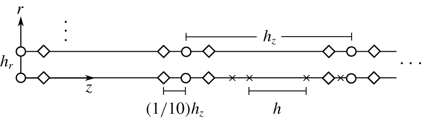
 ${\mathcal{G}}$. Therefore the central difference formula was used for evaluating second-order derivatives containing radial distribution functions. Instead of using the main output points for the central difference calculation, auxiliary points were added on both sides of the main output points, as shown in figure 3, to increase the accuracy.
Illustration of computational grid in this study, including main output points (○), auxiliary points (♢) and interim points ( $\times$). Here
 $h_{z}$ and
 $h_{r}$ are the axial and radial output step sizes, respectively, and
 $h$ is the self-adaptive integration step size.

A global error is needed to validate the simplification made and ensure overall accuracy of the numerical procedures. In the linear regime, equation (3.35) holds exactly. The equality is compromised by simplification and use of numerical methods. Therefore in this study the global relative error was defined as
 $$\begin{eqnarray}\unicode[STIX]{x1D716}=\frac{|(\overline{{\mathcal{P}}})_{cv}-(\overline{{\mathcal{D}}_{\unicode[STIX]{x1D708}}})_{cv}-(\overline{{\mathcal{D}}_{k}})_{cv}-(\boldsymbol{n}\boldsymbol{\cdot }\overline{I})_{cs}|}{\max (|(\overline{{\mathcal{P}}})_{cv}|,|(\overline{{\mathcal{D}}_{\unicode[STIX]{x1D708}}})_{cv}|,|(\overline{{\mathcal{D}}_{k}})_{cv}|,|(\boldsymbol{n}\boldsymbol{\cdot }\overline{I})_{cs}|)}.\end{eqnarray}$$
The mesh numbers were adjusted during the computation to reach a satisfactory error level (here of the order of  $10^{-5}$) to balance computation speed and accuracy.
4 Results and discussion
The aim of the present study is to establish a new analytical framework to clarify the disturbance energy conservation in thermoacoustic devices. In order to demonstrate the usage of the analytical framework, practical cases are considered and a parametric study is conducted to showcase the new perspectives and understanding which would not be possible without the proposed framework.
After a review of actual thermoacoustic devices (e.g. Backhaus & Swift Reference Backhaus and Swift2000; Poese & Garrett Reference Poese and Garrett2000; Dai et al. Reference Dai, Luo, Zhang and Ling2006; Bassem et al. Reference Bassem, Ueda and Akisawa2011; Tijani & Spoelstra Reference Tijani and Spoelstra2011; Yu et al. Reference Yu, Jaworski and Backhaus2012) available in the literature and application constraints such as the temperature of low-grade heat sources, the typical ranges of the parameters are summarized as follows:
 $$\begin{eqnarray}\left.\begin{array}{@{}c@{}}R\in [0.05,0.3]~\text{mm},\quad L\in [10,50]~\text{mm},\quad T_{c}\sim 325~\text{K},\\ T_{h}\in [473,573]~\text{K},\quad \unicode[STIX]{x1D714}\in [40,300]\unicode[STIX]{x03C0}~\text{s}^{-1},\\ p_{0}\in [0.1,3]~\text{MPa},\quad |p^{\prime }|_{\unicode[STIX]{x1D6F4}_{1}}/p_{0}\in [1,10]\,\%,\quad |p^{\prime }|_{\unicode[STIX]{x1D6F4}_{1}}/|(v_{z}^{\prime })_{av}|_{\unicode[STIX]{x1D6F4}_{1}}\in [1,30](\unicode[STIX]{x1D70C}_{0}c)_{\unicode[STIX]{x1D6F4}_{1}},\\ \unicode[STIX]{x1D719}_{vp}\in \left[-{\displaystyle \frac{\unicode[STIX]{x03C0}}{2}},{\displaystyle \frac{\unicode[STIX]{x03C0}}{2}}\right],\end{array}\right\}\end{eqnarray}$$
where  $T_{c}=T_{w}(0)$ and
 $T_{h}=T_{w}(L)$ denote the cold and hot end temperatures. The subscript
 $\unicode[STIX]{x1D6F4}_{1}$ indicates that the flow variable is valued at the inlet surface
 $\unicode[STIX]{x1D6F4}_{1}$ in figure 2. Also,
 $\unicode[STIX]{x1D719}_{vp}$ is a concise notation for the phase difference of
 $(v_{z}^{\prime })_{av}$ and
 $p^{\prime }$ at inlet surface, namely
 $$\begin{eqnarray}\unicode[STIX]{x1D719}_{vp}:=\unicode[STIX]{x1D719}[(v_{z}^{\prime })_{av}]_{\unicode[STIX]{x1D6F4}_{1}}-\unicode[STIX]{x1D719}[p^{\prime }]_{\unicode[STIX]{x1D6F4}_{1}}.\end{eqnarray}$$
The notation  $\unicode[STIX]{x1D719}[f]$ means the phase of a complex quantity
 $f$.
The baseline point was chosen to be roughly the mid-points of the ranges for parameters such as  $R$,
 $L$ and
 $T_{h}$ or a moderate value, such as for
 $p_{0}$, that does not demand extreme operating conditions of the device. In this way, it is possible to show the changes towards both lower and upper bounds of the ranges in the following parametric study. The baseline point was therefore set at
 $R=0.15~\text{mm}$,
 $L=30~\text{mm}$,
 $T_{c}=325~\text{K}$,
 $T_{h}=523~\text{K}$,
 $p_{0}=0.3~\text{MPa}$,
 $|p^{\prime }|_{\unicode[STIX]{x1D6F4}_{1}}/p_{0}=7\,\%$,
 $|(v_{z}^{\prime })_{av}|_{\unicode[STIX]{x1D6F4}_{1}}=3~\text{m}~\text{s}^{-1}$,
 $\unicode[STIX]{x1D719}_{vp}=\unicode[STIX]{x03C0}/36$,
 $\unicode[STIX]{x1D714}=200\unicode[STIX]{x03C0}~\text{s}^{-1}$.
The working fluid was chosen as helium for this parametric study, but the framework is not restricted to this fluid. The dynamic viscosity and thermal conductivity of helium obey the power laws (Touloukian, Liley & Saxena Reference Touloukian, Liley and Saxena1970; Touloukian, Saxena & Hestermans Reference Touloukian, Saxena and Hestermans1975)  $\unicode[STIX]{x1D707}(T)=\unicode[STIX]{x1D707}_{ref}(T/T_{ref})^{n_{\unicode[STIX]{x1D707}}}$ and
 $k(T)=k_{ref}(T/T_{ref})^{n_{k}}$, respectively, where
 $T_{ref}=300~\text{K}$,
 $\unicode[STIX]{x1D707}_{ref}=1.9938\times 10^{-5}~\text{kg}~\text{m}^{-1}~\text{s}^{-1}$,
 $k_{ref}=0.1524~\text{W}~\text{m}^{-1}~\text{K}^{-1}$,
 $n_{\unicode[STIX]{x1D707}}=0.68014$,
 $n_{k}=0.716$.
The global relative error defined in (3.66) in the baseline case was  $5.7\times 10^{-5}$ using an equally spaced 201 (radially) × 51 (axially) mesh, showing the suitability of the approach.
4.1 Parametric study: Womersley number
The Womersley number is the most widely discussed dimensionless number in the research of thermoacoustic devices. This is reasonable since it appears in both the dimensionless momentum equation as  $Wo^{2}$ and the energy equation as
 $Pr\cdot Wo^{2}$. Although
 $\unicode[STIX]{x1D707}=\unicode[STIX]{x1D707}(T_{0})$ and
 $k=k(T_{0})$, the Prandtl number is very weakly dependent on temperature, varying only by 0.01 in the temperature range [325, 525] K. Therefore the Prandtl number is treated as a constant for helium in this study. Parameter
 $Wo^{2}$ being a function of radius, density, frequency and viscosity, can be varied in many ways. In this study, it was varied by changing
 $p_{0}$ and, ultimately,
 $\unicode[STIX]{x1D70C}_{ref}$, given that
 $\unicode[STIX]{x1D735}p_{0}=0$ and
 $p_{0}=\unicode[STIX]{x1D70C}_{ref}R_{g}T_{ref}$. Note that
 $|p^{\prime }|_{\unicode[STIX]{x1D6F4}_{1}}$ needed to be changed to keep
 $p^{\prime \ast }$ constant. It follows that the inlet disturbance energy flux
 $(\boldsymbol{n}\boldsymbol{\cdot }\overline{I})_{\unicode[STIX]{x1D6F4}_{1}}$ used to scale the disturbance energy terms was a linear function of
 $Wo^{2}$.
The terms in the integral disturbance energy balance (3.41) are shown in figure 4 against  $Wo^{2}$. The vertical heights of light, medium and dark grey areas represent, respectively, dimensionless values of the disturbance energy flux
 $(\boldsymbol{n}\boldsymbol{\cdot }\overline{I})_{cs}^{\ast }$, thermal dissipation
 $(\overline{{\mathcal{D}}_{k}})_{cv}^{\ast }$ and viscous dissipation
 $(\overline{{\mathcal{D}}_{\unicode[STIX]{x1D708}}})_{cv}^{\ast }$, of which the sum should equal the thermoacoustic production
 $(\overline{{\mathcal{P}}})_{cv}^{\ast }$ (dashed line in figure 4a). The deviation from the equality, defined as
 $\unicode[STIX]{x1D6E5}^{\ast }=(\overline{{\mathcal{P}}})_{cv}^{\ast }-(\overline{{\mathcal{D}}_{\unicode[STIX]{x1D708}}})_{cv}^{\ast }-(\overline{{\mathcal{D}}_{\unicode[STIX]{x1D708}}})_{cv}^{\ast }-(\boldsymbol{n}\boldsymbol{\cdot }\overline{I})_{cs}^{\ast }$, is plotted in figure 4(b). It can be seen that the difference is four orders of magnitude smaller and hence validates the simplification and assumption made previously. In figure 5,
 $(\overline{{\mathcal{D}}_{\unicode[STIX]{x1D708}}})_{cv}^{\ast }$,
 $(\overline{{\mathcal{D}}_{k}})_{cv}^{\ast }$ and total dissipation
 $(\overline{{\mathcal{D}}}_{k+\unicode[STIX]{x1D708}})_{cv}^{\ast }$ are shown again for better visualization.
The balance of the dimensionless disturbance energy terms against  $Wo^{2}$. (a) The values of the dimensionless thermoacoustic production in the control volume
 $(\overline{{\mathcal{P}}})_{cv}^{\ast }$ (– – –), viscous dissipation
 $(\overline{{\mathcal{D}}_{\unicode[STIX]{x1D708}}})_{cv}^{\ast }$ (▪), thermal dissipation
 $(\overline{{\mathcal{D}}_{\unicode[STIX]{x1D708}}})_{cv}^{\ast }$ (

 $(\boldsymbol{n}\boldsymbol{\cdot }\overline{I})_{cs}^{\ast }$ (

 $\unicode[STIX]{x1D6E5}^{\ast }=(\overline{{\mathcal{P}}})_{cv}^{\ast }-(\overline{{\mathcal{D}}_{\unicode[STIX]{x1D708}}})_{cv}^{\ast }-(\overline{{\mathcal{D}}_{\unicode[STIX]{x1D708}}})_{cv}^{\ast }-(\boldsymbol{n}\boldsymbol{\cdot }\overline{I})_{cs}^{\ast }$.

The changes of (a) the dimensionless thermal dissipation  $(\overline{{\mathcal{D}}_{k}})_{cv}^{\ast }$ (——), viscous dissipation
 $(\overline{{\mathcal{D}}_{\unicode[STIX]{x1D708}}})_{cv}^{\ast }$ (– – –) and total dissipation
 $(\overline{{\mathcal{D}}}_{k+\unicode[STIX]{x1D708}})_{cv}^{\ast }$ (— ⋅ —) and (b) the viscous dissipation (▪) and thermal dissipation (

 $Wo^{2}$.

A straightforward yet important conclusion from figure 5(b) is that the relative importance of viscous and thermal dissipation, which can be defined as the percentages  $(\overline{{\mathcal{D}}_{\unicode[STIX]{x1D708}}})_{cv}/(\overline{{\mathcal{D}}}_{k+\unicode[STIX]{x1D708}})_{cv}$ and
 $(\overline{{\mathcal{D}}_{k}})_{cv}/(\overline{{\mathcal{D}}}_{k+\unicode[STIX]{x1D708}})_{cv}$, respectively, shifts with
 $Wo^{2}$. When other conditions are maintained, viscous dissipation is more significant at low
 $Wo^{2}$ while thermal dissipation is the main loss mechanism at high
 $Wo^{2}$. This is because
 $Wo$, according to (3.20), represents the channel radius relative to boundary-layer thickness; as the relative radius becomes larger, the portion of main flow, which has little velocity gradient, also grows. Hence the relative viscous dissipation decreases. For the temperature profile, no oscillation is allowed (i.e.
 $T^{\prime }=0$) at the wall due to the implicit assumption of its infinite heat capacity originated from the boundary condition
 $T(R,z)=T_{w}(z)$. As the relative radius becomes larger compared to the thermal boundary layer, the wall’s ability to ‘smooth out’ the temperature profile decreases as shown in figure 6: the magnitude of temperature oscillation becomes larger and so does its radial gradient. This leads to a surge of thermal dissipation. In summary, figure 5(b) points out the main loss mechanism to tackle when building thermoacoustic devices.
The changes of the magnitude of (a) the dimensionless temperature fluctuation  $|T^{\prime \ast }|$ and (b) the dimensionless radial derivative of temperature fluctuation
 $|\unicode[STIX]{x2202}T^{\prime \ast }/\unicode[STIX]{x2202}r^{\ast }|$ against dimensionless radial position
 $r/R$ at mid-axial position
 $z=L/2$ for four different
 $Wo^{2}$:
 $Wo^{2}=0.06$ (— ⋅ —),
 $Wo^{2}=0.19$ (——),
 $Wo^{2}=0.32$ (– – –),
 $Wo^{2}=1.9$ (
 $\cdots \cdots$).

The changes of  $(\overline{{\mathcal{P}}})_{cv}^{\ast }$,
 $(\overline{{\mathcal{D}}_{\unicode[STIX]{x1D708}}})_{cv}^{\ast }$,
 $(\overline{{\mathcal{D}}_{k}})_{cv}^{\ast }$ and
 $(\boldsymbol{n}\boldsymbol{\cdot }\overline{I})_{cs}^{\ast }$ with
 $Wo^{2}$ can be divided into four regions by three critical values of
 $Wo^{2}$ as labelled in figure 4. With
 $Wo^{2}$ increasing from 0,
 $(\boldsymbol{n}\boldsymbol{\cdot }\overline{I})_{cs}^{\ast }$ grows faster than
 $(\overline{{\mathcal{P}}})_{cv}^{\ast }$. Given
 $(\boldsymbol{n}\boldsymbol{\cdot }\overline{I})_{cs}^{\ast }=(\overline{{\mathcal{P}}})_{cv}^{\ast }-(\overline{{\mathcal{D}}}_{k+\unicode[STIX]{x1D708}})_{cv}^{\ast }$, this faster increase of acoustic output clearly benefits from the initial drop of total dissipation as shown in figure 5(a) from 0 to
 $C_{1}$;
 $C_{1}$ is
 $Wo^{2}$ where total dissipation reaches a minimum. It follows that
 $C_{1}$ is also the position where
 $(\overline{{\mathcal{P}}})_{cv}^{\ast }$ and
 $(\boldsymbol{n}\boldsymbol{\cdot }\overline{I})_{cs}^{\ast }$ have parallel tangent lines, i.e.
 $\text{d}(\overline{{\mathcal{P}}})_{cv}^{\ast }=\text{d}(\boldsymbol{n}\boldsymbol{\cdot }\overline{I})_{cs}^{\ast }$. Formally,
 $C_{1}$ is defined as
 $$\begin{eqnarray}C_{1}=\min (Wo^{2}:\text{d}(\overline{{\mathcal{D}}}_{k+\unicode[STIX]{x1D708}})_{cv}^{\ast }=0),\end{eqnarray}$$
where the  $\min (\,)$ function ensures the first such
 $Wo^{2}$. The physical meaning of
 $C_{1}$ is
 $Wo^{2}$ where thermoacoustic production starts to grow faster than acoustic output and where the system has a minimum loss.
On continuing to increase  $Wo^{2}$, the total dissipation starts to pick up and the rate of change of the production exceeds that of the disturbance energy flux and the second critical value
 $C_{2}$ can be defined as
 $$\begin{eqnarray}C_{2}=\min \left(Wo^{2}:\text{d}\frac{(\boldsymbol{n}\boldsymbol{\cdot }\overline{I})_{cs}^{\ast }}{(\overline{{\mathcal{P}}})_{cv}^{\ast }}=0\right).\end{eqnarray}$$
Equivalently,  $C_{2}$ is also where
 $\text{d}\text{ln}(\overline{{\mathcal{P}}})_{cv}^{\ast }=\text{d}\text{ln}(\boldsymbol{n}\boldsymbol{\cdot }\overline{I})_{cs}^{\ast }$. It is clear that this ratio,
 $$\begin{eqnarray}\unicode[STIX]{x1D702}:=\frac{(\boldsymbol{n}\boldsymbol{\cdot }\overline{I})_{cs}^{\ast }}{(\overline{{\mathcal{P}}})_{cv}^{\ast }},\end{eqnarray}$$
is the efficiency of the conversion from thermal energy to acoustic energy. Then  $C_{2}$ is
 $Wo^{2}$ where maximum efficiency is reached. This new definition of ‘true’ thermoacoustic efficiency reflects only the energy conversion between different aspects of the disturbance and does not concern any steady-state physical process. The changes of thermoacoustic efficiency are better visualized in figure 7.
The changes of the thermoacoustic efficiency  $\unicode[STIX]{x1D702}$ against
 $Wo^{2}$.

On further increasing  $Wo^{2}$, it can be seen that both thermoacoustic production and dissipation (mainly thermal) rise sharply. It is clear in figure 4(a) that
 $(\boldsymbol{n}\boldsymbol{\cdot }\overline{I})_{cs}^{\ast }$ has a turning point
 $C_{3}$, i.e.
 $\text{d}(\boldsymbol{n}\boldsymbol{\cdot }\overline{I})_{cs}^{\ast }=0$. It follows that
 $C_{3}$ is also the position where
 $(\overline{{\mathcal{P}}})_{cv}^{\ast }$ and
 $(\overline{{\mathcal{D}}}_{k+\unicode[STIX]{x1D708}})_{cv}^{\ast }$ have the same rate of change, namely
 $\text{d}(\overline{{\mathcal{P}}})_{cv}^{\ast }=\text{d}(\overline{{\mathcal{D}}}_{k+\unicode[STIX]{x1D708}})_{cv}^{\ast }$. Formally,
 $$\begin{eqnarray}C_{3}=\min (Wo^{2}:\text{d}(\boldsymbol{n}\boldsymbol{\cdot }\overline{I})_{cs}^{\ast }=0).\end{eqnarray}$$
The physical meaning of  $C_{3}$ is
 $Wo^{2}$ where
 $(\boldsymbol{n}\boldsymbol{\cdot }\overline{I})_{cs}^{\ast }$ reaches a maximum and also where dissipation starts to grow faster than production.
It follows that the four distinct regions are
(i)
 $Wo^{2}<C_{1}$: total dissipation decreases, the efficiency of the device rises and energy flux grows faster than production;
(ii)
$C_{1}<Wo^{2}<C_{2}$: efficiency rises, total dissipation rises and production grows faster than energy flux;(iii)
$C_{2}<Wo^{2}<C_{3}$: efficiency drops but production grows faster than dissipation; and(iv)
$Wo^{2}>C_{3}$: dissipation rises faster than production.


4.2 Parametric study: Helmholtz number
The Helmholtz number represents the length of the channel relative to the wavelength. A thermoacoustic regenerator is generally very short compared with the wavelength:  $He\sim O(0.01)$. In this section, the effects of
 $He$ on disturbance energy budget are studied by varying the channel length
 $L$ while maintaining other conditions.
The terms in the disturbance energy balance equation are shown in figure 8(a) against the Helmholtz number. Similar to figure 4, the heights of the light, medium and dark grey areas represent dimensionless values of disturbance energy flux  $(\boldsymbol{n}\boldsymbol{\cdot }\overline{I})_{cs}^{\ast }$, thermal dissipation
 $(\overline{{\mathcal{D}}_{k}})_{cv}^{\ast }$ and viscous dissipation
 $(\overline{{\mathcal{D}}_{\unicode[STIX]{x1D708}}})_{cv}^{\ast }$, respectively, of which the sum should equal the thermoacoustic production
 $(\overline{{\mathcal{P}}})_{cv}^{\ast }$ (dashed line in figure 8). The drop of thermoacoustic production with
 $He$ is expected because a larger length reduces the temperature gradient. Compared to figure 4, no turning point of
 $(\boldsymbol{n}\boldsymbol{\cdot }\overline{I})_{cs}^{\ast }$ is observed in the computed range;
 $(\boldsymbol{n}\boldsymbol{\cdot }\overline{I})_{cs}^{\ast }$ decreases monotonically. This result seems to suggest that shorter regenerators are always preferable; however, in practice, the conductivity of the material needs to be taken into account. If the length is too short, most of the heat input would be conducted through the solid wall instead of being transferred to the fluid. The deviation from equality
 $\unicode[STIX]{x1D6E5}^{\ast }$ against
 $He$ is shown in figure 8(b); again excellent agreement is seen.
The balance of dimensionless disturbance energy terms against  $He$. (a) The values of the dimensionless thermoacoustic production in the control volume
 $(\overline{{\mathcal{P}}})_{cv}^{\ast }$ (– – –), viscous dissipation
 $(\overline{{\mathcal{D}}_{\unicode[STIX]{x1D708}}})_{cv}^{\ast }$ (▪), thermal dissipation
 $(\overline{{\mathcal{D}}_{\unicode[STIX]{x1D708}}})_{cv}^{\ast }$ (

 $(\boldsymbol{n}\boldsymbol{\cdot }\overline{I})_{cs}^{\ast }$ (

 $\unicode[STIX]{x1D6E5}^{\ast }=(\overline{{\mathcal{P}}})_{cv}^{\ast }-(\overline{{\mathcal{D}}_{\unicode[STIX]{x1D708}}})_{cv}^{\ast }-(\overline{{\mathcal{D}}_{\unicode[STIX]{x1D708}}})_{cv}^{\ast }-(\boldsymbol{n}\boldsymbol{\cdot }\overline{I})_{cs}^{\ast }$.

The minimum total dissipation  $C_{1}$ was obtained at
 $He=0.014$, a combined effect of decreasing thermal dissipation and rising viscous dissipation with
 $He$ as shown in figure 9(a). Hence the main loss mechanism for a long regenerator is friction while for short ones it is irreversible heat conduction as visualized in figure 9(b).
The changes of (a) the dimensionless thermal dissipation  $(\overline{{\mathcal{D}}_{k}})_{cv}^{\ast }$ (——), viscous dissipation
 $(\overline{{\mathcal{D}}_{\unicode[STIX]{x1D708}}})_{cv}^{\ast }$ (– – –) and total dissipation
 $(\overline{{\mathcal{D}}}_{k+\unicode[STIX]{x1D708}})_{cv}^{\ast }$ (— ⋅ —) and (b) the viscous dissipation (▪) and thermal dissipation (

 $He$.

The changes of the magnitude of (a) the dimensionless temperature fluctuation  $|T^{\prime \ast }|$ and (b) the dimensionless entropy fluctuation
 $|s^{\prime \ast }|$ against dimensionless axial position
 $z/L$ on the axis
 $r=0$ for four different
 $He$:
 $He=0.008$ (— ⋅ —),
 $He=0.012$ (——),
 $He=0.019$ (– – –),
 $He=0.031$ (
 $\cdots \cdots$).

The viscous dissipation is expected to rise with increasing  $He$ because at high
 $He$, the boundary layer extends further in the axial direction, consequently leading to more dissipation. The decline of thermal dissipation with increasing
 $He$ can be traced back to
 $T^{\prime \ast }$ as shown in figure 10(a). It is clear that the magnitude of
 $T^{\prime \ast }$ diminishes as
 $He$ increases and, given that
 $R$ is constant, so does
 $|\unicode[STIX]{x2202}T^{\prime \ast }/\unicode[STIX]{x2202}r^{\ast }|$. According to (3.44), the thermal dissipation also diminishes.
The thermoacoustic production, by (3.47), depends on  $|s^{\prime \ast }|$,
 $|v_{z}^{\prime \ast }|$ and
 $\unicode[STIX]{x1D719}_{vs}$. The main contributor in this case was
 $|s^{\prime \ast }|$, which also decreases with increasing
 $He$ as shown in figure 10(b). This is because the solutions of
 $T^{\prime \ast }$ and
 $s^{\prime \ast }$ are
 $$\begin{eqnarray}\displaystyle & \displaystyle T^{\prime \ast }=\frac{1-{\mathcal{H}}_{k}}{\unicode[STIX]{x1D70C}_{0}^{\ast }}p^{\prime \ast }-\frac{1}{He^{2}}\frac{1}{\unicode[STIX]{x1D70C}_{0}^{\ast }}\frac{\text{d}T_{w}^{\ast }}{\text{d}z^{\ast }}\frac{(1-{\mathcal{H}}_{k})-Pr(1-{\mathcal{H}}_{\unicode[STIX]{x1D708}})}{1-Pr}\frac{\text{d}p^{\prime \ast }}{\text{d}z^{\ast }}, & \displaystyle\end{eqnarray}$$
 $$\begin{eqnarray}\displaystyle & \displaystyle s^{\prime \ast }=\frac{-{\mathcal{H}}_{k}}{\unicode[STIX]{x1D70C}_{0}^{\ast }T_{0}^{\ast }}p^{\prime \ast }-\frac{1}{He^{2}}\frac{1}{\unicode[STIX]{x1D70C}_{0}^{\ast }T_{0}^{\ast }}\frac{\text{d}T_{w}^{\ast }}{\text{d}z^{\ast }}\frac{(1-{\mathcal{H}}_{k})-Pr(1-{\mathcal{H}}_{\unicode[STIX]{x1D708}})}{1-Pr}\frac{\text{d}p^{\prime \ast }}{\text{d}z^{\ast }}. & \displaystyle\end{eqnarray}$$
It can be seen the second parts of the solutions contain  $\text{d}T_{w}^{\ast }/\text{d}z^{\ast }$; they are the temperature and entropy fluctuation originated from the temperature gradient. In the parametric study,
 $\text{d}T_{w}^{\ast }/\text{d}z^{\ast }$ are identical across
 $He$: the same cold and hot temperature varying linearly from 0 to 1. It is
 $He$ that accounts for the temperature gradient changes in the dimensionless domain. Since both solutions contain the inverse of
 $He$, the magnitudes drop with increasing
 $He$.
The changes of the thermoacoustic efficiency against  $He$.

The thermoacoustic efficiency  $\unicode[STIX]{x1D702}$ is shown against
 $He$ in figure 11. Although there exists the highest efficiency
 $C_{2}$ at
 $He=0.012$, the change of the efficiency is rather insensitive to
 $He$ compared with that against
 $Wo^{2}$ in figure 7. This indicates that as long as
 $He$ is small (
 ${\sim}O(0.01)$), the effect of the channel length (and consequently temperature gradient) on the efficiency is less important than the effects of shear and heat transfer in the radial direction.
As mentioned previously, the wave growth decreases monotonically with larger  $He$; in practice the choice of
 $\unicode[STIX]{x1D714}$ and
 $L$ should ideally be such that the resulting
 $He$ falls to the left of
 $C_{1}$, i.e.
 $He<C_{1}$, taking advantage of both high efficiency and high output.
4.3 Two-dimensional variation
Up to this point, the global values (volume integral  $(\overline{{\mathcal{P}}})_{cv}^{\ast }$,
 $(\overline{{\mathcal{D}}_{k}})_{cv}^{\ast }$,
 $(\overline{{\mathcal{D}}_{\unicode[STIX]{x1D708}}})_{cv}^{\ast }$ and surface integral
 $(\boldsymbol{n}\boldsymbol{\cdot }\overline{I})_{cs}^{\ast }$) and the integral form of the disturbance energy balance relation (3.35) have been used. In this section, the differential form of disturbance energy (2.27) is employed to analyse the two-dimensional variation of the point-based values
 $(\overline{{\mathcal{P}}})^{\ast }$,
 $(\unicode[STIX]{x1D735}\boldsymbol{\cdot }\overline{I})^{\ast }$,
 $(\overline{{\mathcal{D}}_{k}})^{\ast }$ and
 $(\overline{{\mathcal{D}}_{\unicode[STIX]{x1D708}}})^{\ast }$.
Compared with previous one-dimensional models, one of the highlights of this work is that the problem is considered in an axisymmetric cylindrical domain. Hence, this work is capable of showing the two-dimensional variation of the disturbance energy terms against radial and axial location. The profiles of  $(\overline{{\mathcal{P}}})^{\ast }$,
 $(\unicode[STIX]{x1D735}\boldsymbol{\cdot }\overline{I})^{\ast }$,
 $(\overline{{\mathcal{D}}_{k}})^{\ast }$ and
 $(\overline{{\mathcal{D}}_{\unicode[STIX]{x1D708}}})^{\ast }$ are given in figure 12. The vertical axis is the dimensionless radius
 $r^{\ast }=r/R$, where
 $r^{\ast }=0$ represents the axis and
 $r^{\ast }=1$ is the wall.
The profiles of the cycle-averaged (a) dimensionless thermoacoustic production  $(\overline{{\mathcal{P}}})^{\ast }$, (b) viscous dissipation
 $(\overline{{\mathcal{D}}_{\unicode[STIX]{x1D708}}})^{\ast }$, (c) disturbance energy flux density
 $(\unicode[STIX]{x1D735}\boldsymbol{\cdot }\overline{I})^{\ast }$ and (d) thermal dissipation
 $(\overline{{\mathcal{D}}_{k}})^{\ast }$ at six axial locations:
 $z/L=0.02$, 0.2, 0.4, 0.6, 0.8, 0.98 which are denoted by ○, ▫, ♢, ▵, ▹, ◃, respectively, at the baseline point.

The focus first is on the radial variation. At the wall,  $(\overline{{\mathcal{P}}})^{\ast }$ is zero because
 $v_{z}^{\prime \ast }$ is zero (no-slip boundary condition). Both
 $(\overline{{\mathcal{D}}_{\unicode[STIX]{x1D708}}})^{\ast }$ and
 $(\overline{{\mathcal{D}}_{k}})^{\ast }$ are significant because
 $|\unicode[STIX]{x2202}T^{\prime \ast }/\unicode[STIX]{x2202}r^{\ast }|$ and
 $|\unicode[STIX]{x2202}v_{z}^{\prime \ast }/\unicode[STIX]{x2202}r^{\ast }|$ are both large at the wall. Consequently, the near-wall region actually sees a negative energy flux density
 $(\unicode[STIX]{x1D735}\boldsymbol{\cdot }\overline{I})^{\ast }=(\overline{{\mathcal{P}}})^{\ast }-(\overline{{\mathcal{D}}}_{k+\unicode[STIX]{x1D708}})^{\ast }<0$, representing a wave decay. The
 $(\unicode[STIX]{x1D735}\boldsymbol{\cdot }\overline{I})^{\ast }=0$ level mark is shown in figure 12(c) for clearer visualization. It is interesting to realize that even for thermoacoustic devices designed to amplify waves, a small region of wave decay always exists. The near-wall wave decay also provides support to the conclusion in § 4.1 that overly small
 $Wo^{2}$ is not optimal. On the axis,
 $(\overline{{\mathcal{P}}})^{\ast }$ reaches the maximum while dissipation is zero (axisymmetric condition) and hence
 $(\unicode[STIX]{x1D735}\boldsymbol{\cdot }\overline{I})^{\ast }=(\overline{{\mathcal{P}}})^{\ast }$ on the axis. The fact that wave growth is uneven in the radial direction implies the presence of radial mixing loss associated with fluid near both ends entering and leaving the channels during oscillation.
With regard to the axial variation, it is too simplistic to assume the shapes of the profiles are self-similar. Take  $\overline{{\mathcal{P}}}$ for example. Each profile is normalized using respective values on the axis as shown in figure 13. It can be seen that the profiles are almost self-similar but not quite. This is because radial distribution functions contain the local viscous and thermal boundary-layer thicknesses
 $\unicode[STIX]{x1D6FF}_{\unicode[STIX]{x1D708}}$ and
 $\unicode[STIX]{x1D6FF}_{k}$, which ultimately depend on
 $T(z)$.
The profiles of the thermoacoustic production normalized by its value on the axis  $\overline{{\mathcal{P}}}/(\overline{{\mathcal{P}}})_{r\,=\,0}$ against dimensionless radial position
 $r/R$ at six axial locations:
 $z/L=0.02$, 0.2, 0.4, 0.6, 0.8, 0.98 which are denoted by ○, ▫, ♢, ▵, ▹, ◃, respectively, at the baseline point.

The axial changes were monotonic:  $(\overline{{\mathcal{P}}})^{\ast }$,
 $(\overline{{\mathcal{D}}_{k}})^{\ast }$ and
 $(\unicode[STIX]{x1D735}\boldsymbol{\cdot }\overline{I})^{\ast }$ decreased as the axial location moves towards the hot end; on the contrary,
 $(\overline{{\mathcal{D}}_{\unicode[STIX]{x1D708}}})^{\ast }$ increased. Recalling equations (3.46) and (3.44), the changes of
 $(\overline{{\mathcal{D}}_{k}})^{\ast }$ and
 $(\overline{{\mathcal{D}}_{\unicode[STIX]{x1D708}}})^{\ast }$ are readily explained by the profiles of
 $|\unicode[STIX]{x2202}T^{\prime \ast }/\unicode[STIX]{x2202}r^{\ast }|$ and
 $|\unicode[STIX]{x2202}v_{z}^{\prime \ast }/\unicode[STIX]{x2202}r^{\ast }|$ as shown in figure 14. Note that although
 $k(T_{w}(z))$ increased with axial location (actually
 $k(L)=1.41k(0)$), the factor
 $k^{\ast }(1/T_{0}^{\ast })$ in (3.44) actually decreased with axial location given the power law
 $k\propto T^{0.716}$ as mentioned previously.
The profiles of the magnitude of (a) the dimensionless radial derivative of temperature fluctuation  $|\unicode[STIX]{x2202}T^{\prime \ast }/\unicode[STIX]{x2202}r^{\ast }|$ and (b) the dimensionless radial derivative of axial velocity fluctuation
 $|\unicode[STIX]{x2202}v_{z}^{\prime \ast }/\unicode[STIX]{x2202}r^{\ast }|$ against dimensionless radial position
 $r/R$ at six axial locations:
 $z/L=0.02$, 0.2, 0.4, 0.6, 0.8, 0.98, which are denoted by ○, ▫, ♢, ▵, ▹, ◃, respectively, at the baseline point.

By referring to the thermoacoustic production (3.47), the effect of  $\text{d}T_{0}^{\ast }/\text{d}z^{\ast }$ vanished here by the choice of linear temperature distribution. The factor
 $-\overline{s^{\prime \ast }v_{z}^{\prime \ast }}$ is the specific entropy transported by the volumetric flow rate per unit area per unit time. The profiles of
 $-\overline{s^{\prime \ast }v_{z}^{\prime \ast }}$ are shown in figure 15. It is clear that
 $-\overline{s^{\prime \ast }v_{z}^{\prime \ast }}$ increased as axial position moves towards the hot end. However, this trend was reversed by
 $\unicode[STIX]{x1D70C}_{0}^{\ast }$, which decreases with
 $z$.
The profiles of the cycle-averaged product of dimensionless fluctuating entropy and axial velocity  $-\overline{s^{\prime \ast }v_{z}^{\prime \ast }}$ against dimensionless radial position
 $r/R$ at six axial locations:
 $z/L=0.02$, 0.2, 0.4, 0.6, 0.8, 0.98, which are denoted by ○, ▫, ♢, ▵, ▹, ◃, respectively, at the baseline point.

In summary, it has been shown that there is a near-wall wave decay region and the two-dimensional variation of  $(\overline{{\mathcal{P}}})^{\ast }$,
 $(\unicode[STIX]{x1D735}\boldsymbol{\cdot }\overline{I})^{\ast }$,
 $(\overline{{\mathcal{D}}_{k}})^{\ast }$ and
 $(\overline{{\mathcal{D}}_{\unicode[STIX]{x1D708}}})^{\ast }$ can be summarized as similar radial profiles and monotonic axial changes.
5 Conclusions
In this work, a new analytical framework has been developed to better understand the disturbance energy balance in thermoacoustic devices. In this framework, a thermoacoustic production term is newly proposed which directly quantifies the generation or consumption of disturbance energy from an imposed temperature gradient. An extended disturbance energy flux term, in place of acoustic intensity, is defined to account for wave growth or decay in thermoacoustic devices. The viscous and thermal dissipation solely resulting from the gradients of fluctuating velocity and temperature are obtained. The disturbance energy balance relation is then established, stating that the wave growth equals thermoacoustic production less viscous and thermal dissipation. The proposed framework enables a new analytical perspective using these four disturbance energy terms and the changes of the balance itself. Both the differential and integral forms of the disturbance energy balance equation are given.
In this study, the framework has been implemented in an axisymmetric cylindrical domain. The governing equations have been non-dimensionalized and the driving dimensionless parameters, namely the Womersley number, the Helmholtz number and the Prandtl number, are revealed. The well-accepted Rott’s assumptions were reinterpreted using order-of-magnitude analysis. The disturbance energy terms are then simplified by extending Rott’s assumptions and taking advantage of boundary conditions. The flow variables have been solved analytically in the radial direction and numerically in the axial direction. A global error of the disturbance energy balance has been defined to validate the assumptions made and the numerical scheme used in this study. Compared with previous one-dimensional models, one of the highlights of this work is the ability to show two-dimensional variations. It has been found that the disturbance energy terms have similar but not strictly self-similar radial shapes and monotonic axial changes. It has been discovered that the wave always decays in the region close to wall, which implies extra mixing loss that one-dimensional models fail to see.
In order to showcase the new perspectives enabled by the proposed framework, a parametric study of the Womersley and Helmholtz numbers has been conducted. The study is not intended to be exhaustive but to demonstrate how new physical insights and design guidelines can be obtained from the disturbance energy balance relation. The findings are:
(i) The Womersley and Helmholtz numbers can be interpreted as the channel radius relative to boundary-layer thickness and the channel length relative to the wavelength, respectively. It has been found that for a relatively wide channel (represented by a large Womersley number) or short channel (small Helmholtz number), the major loss mechanism is thermal dissipation; in both cases this is due to substantial temperature fluctuation. For a relatively narrow or long regenerator channel, viscous dissipation dominates. The significance of thermal dissipation in thermoacoustic devices has become clear for the first time.
(ii) This paper answers the question as to what is the ‘true’ thermoacoustic efficiency. A new thermoacoustic efficiency has been defined as the ratio of wave growth to thermoacoustic disturbance production; it reflects only the energy conversion between different aspects of the disturbance and does not concern any steady-state physical process.
(iii) The change of thermoacoustic efficiency is rather insensitive to the Helmholtz number compared to the Womersley number. This indicates that as long as the regenerator is short compared to the wavelength (
$He\sim O(0.01)$), the effect of the channel length (and consequently temperature gradient) on the efficiency is less important than the effects of momentum and thermal diffusion in the radial direction.(iv) Three critical design values are identified: the minimum of dimensionless total dissipation, the maximum of thermoacoustic efficiency and the maximum of dimensionless wave growth. These three critical values divided the parameter space into four regimes; a designer can wisely pick a combination of geometry, wave properties and working conditions according to the preference of efficiency, output and loss.

Declaration of interests
The authors report no conflict of interest.