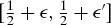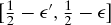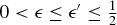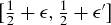


The Condorcet Jury Theorem (CJT) looks back on a remarkable career. Discovered by Nicolas de Caritat, Marquis de Condorcet, in 1785, first proved formally by Laplace in 1812 (Ben-Yashar and Paroush 2007: 190), then long forgotten and finally rediscovered by Duncan Black (Black Reference Black1958, Grofman and Feld Reference Grofman and Feld1988), the CJT has now taken centre stage in epistemic conceptions of democracy and in debates in social epistemology. Propelled by claims in the popular literature that crowds can be ‘wise’ (Surowiecki Reference Surowiecki2004) and mobs ‘smart’ (Rheingold Reference Rheingold2002), the CJT is now again widely discussed across various disciplines, even beyond academic circles. This career is surprising for a theorem that – in its basic form and applied naively – rests on implausible premises and leads to implausible conclusions, as we will show.
Roughly speaking, the CJT arrives at two conclusions concerning a group decision between two alternatives, where one alternative is objectively correct or better. First, the larger the group gets, the more likely is a correct majority decision. This is the CJT's non-asymptotic conclusion. Second, the probability of a correct majority decision converges to one as the group size tends to infinity. This is the CJT's asymptotic conclusion. Put roughly: larger groups make better decisions, and very large groups are infallible. It is worth reflecting on these results. While we think that the non-asymptotic conclusion is plausible for many setups and can be defended, the asymptotic conclusion is more than dubious. If the asymptotic conclusion applied directly to modern democracies with their large populations, these democracies would be essentially infallible when making decisions between two alternatives by simple majority.
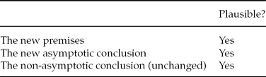
What went wrong? The CJT rests on two central premises. Stated roughly, the first premise is that the voters vote independently from each other, and the second premise is that each voter is competent, i.e. is more likely to vote for the correct than the incorrect alternative (both premises will later be spelt out more carefully and then revised). Our negative finding is the implausibility of the premises – specifically, the independence premise – which explains the implausible asymptotic conclusion of infallible large groups. The non-asymptotic conclusion that larger groups perform better, by contrast, is plausible, but is currently relying on implausible premises and therefore left hanging without support. Our negative finding can be summed up in a table:
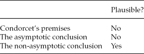
Our positive finding consists in a revision of Condorcet's premises. The new, more plausible premises lead to the new, plausible asymptotic conclusion that large groups are fallible. They also offer a justification for the old non-asymptotic conclusion, which previously rested on implausible premises. This will put us in a new position:
The literature contains several other modifications of the original theorem. Some of them improve the theorem's conclusions; yet they revise the premises in ways quite different from ours. We briefly review some of these proposals, and contrast them with our own approach, whose premises are philosophically transparent and defensible.
In fact, the classical CJT rests on yet another assumption, which is implicit in the classical framework: people vote sincerely. This implicit premise is no less problematic than the explicit premises. It was uncovered in the 1990s and is being addressed in an ongoing literature. While much progress has already been achieved along this dimension of strategic voting, the problems underlying the explicit premises – specifically, the premise of independent voting – have not yet been understood in a systematic and foundational way.
Most believe that ‘something’ is wrong with Condorcet's premises, but confusion prevails over how best to conceptualize and solve the problem. Addressing this is important also because the new literature on strategic voting and the CJT, despite the progress over the classical CJT literature along the strategic voting dimension, still rests on the problematic independence premise (applied now to voters' private information rather than their votes). Since the strategic voting aspect is orthogonal to the problems related to Condorcet's explicit premises, it is not addressed in the present analysis, though a few more remarks on strategic voting will follow below.
This introduction is followed by seven sections. Section 1 begins by laying out the classical CJT as it is often cited and applied in the contemporary literature. In section 2 we show that the classical independence assumption cannot be justified and will typically be false, and propose a new, improved independence assumption. The revision of the independence assumption requires using a new competence assumption, which is provided in section 3. Section 4 contains our first positive result, a new jury theorem based on the new independence and competence assumptions. We point out that the classical CJT is nothing but a special case of our new theorem. In section 5 we highlight two important implications of the new theorem for the theory of epistemic democracy: deliberation and education may be crucial for the epistemic performance of groups, whereas the classical CJT suggests that they are inessential – since ‘crowds are infallible’ even without them – or even dangerous – since deliberation threatens voter independence. Section 6 presents our second positive result, a jury theorem for interchangeable (‘indistinguishable’) voters, generalizing Krishna Ladha's (Reference Ladha1993) seminal jury theorem. Section 7 draws conclusions.
1. CONDORCET'S JURY THEOREM RECAPITULATED
We begin by stating and explaining the classical CJT before criticizing its assumptions in the next sections. The first statement can be found in Condorcet (Reference Condorcet1785), a translation of most parts in Sommerlad and McLean (Reference Sommerlad and McLean1989). The theorem has been stated in many variants; an influential one is provided by Grofman et al. (Reference Grofman and Feld1983). Among the most important applications in political philosophy are Grofman and Feld's (Reference Grofman and Feld1988) use of the CJT to interpret Rousseau's ‘general will’ (cf. Estlund et al. Reference Estlund, Waldron, Grofman and Feld1989) and, of course, the link between the CJT and epistemic conceptions of democracy (Cohen Reference Cohen1986, Gaus Reference Gaus1997, List and Goodin Reference List and Goodin2001, Estlund Reference Estlund2008). A link between the CJT, judgement aggregation and social epistemology is offered by Bovens and Rabinowicz (Reference Bovens and Rabinowicz2006) and List (Reference List2005). Several important generalizations of the classical CJT have been proposed. For instance, Owen et al. (Reference Owen, Grofman and Feld1989) prove that the asymptotic part also holds if judges are heterogeneous in competence, and Romeijn and Atkinson (Reference Romeijn and Atkinson2011) analyse cases of unknown competence. Different papers recognize that independence is hard to meet and/or prove jury theorems which weaken the independence assumption (e.g. Nitzan and Paroush Reference Nitzan and Paroush1984, Shapley and Grofman Reference Shapley and Grofman1984, Boland Reference Boland, Proschan and Tong1989, Boland et al. Reference Boland1989, Berg Reference Berg1993, Estlund Reference Estlund1994, Kaniovski Reference Kaniovski2010, Spiekermann and Goodin Reference Goodin and Spiekermann2012).
Among the most systematic treatments of independence violations so far is the work of Ladha (Reference Ladha1992, Reference Ladha1993, Reference Ladha1995), who shows that shared information and other common causes typically lead to correlated votes, even if the jurors do not influence each other directly. He proves new jury theorems which considerably weaken the independence assumption. In the penultimate section we show that our jury theorem is related to and can be used to generalize Ladha's (Reference Ladha1993) jury theorem for interchangeable voters, which draws on de Finetti's Theorem.
Despite mathematical achievements, previous analyses of voter dependence do not tackle the conceptual core of the problem and provide little guidance for institutional design. The question of the origin of independence violations has remained obscure and unmodelled. For this reason the proposed independence relations are hard to interpret or justify, and their empirical plausibility is difficult to assess. Among the proposed independence relations, many seem suspicious in that they retain the implausible asymptotic conclusion (a notable exception being Ladha Reference Ladha1995, Proposition 4), and many seem ad hoc since they take the votes to be jointly distributed in certain special, mathematically convenient ways. To obtain a systematic account of voter (in)dependence, one must understand how the causal interactions in the voters' institutional and deliberative environment create probabilistic dependence. We offer such a methodological analysis for the first time by developing a general network-theoretic account of voter dependence. It is inspired by, but significantly goes beyond Dietrich and List (Reference Dietrich and List2004) and Dietrich (Reference Dietrich2008), who also employ causal network reasoning but only focus on special cases of independence violations.
We now give a precise rendering of the classical CJT. Let there be a group of individuals, labelled i = 1, 2, 3, . . . The size of the group (electorate) is any number n, which we assume to be odd to avoid ties under majority voting.Footnote 2 The group has to decide between two alternatives, labelled 0 and 1. Exactly one of these alternatives is ‘correct’, ‘right’ or ‘better’.Footnote 3 We will use the attribute ‘correct’ from now on. The correct alternative is called the state (of the world) and is typically denoted x. The state is generated by a random variable x, taking the values 0 and 1, each with positive probability. Each person votes for one alternative, abstentions are not allowed. For each voter i we consider an event Ri, the event that voter i votes correctly. (Some authors take the votes rather than the correct voting events Ri as primitives of the model. This makes no difference since the votes and the correct voting events are interdefinable given the state x.Footnote 4) We write Mn for the event that a majority of an n-member electorate votes correctly.Footnote 5
Classical Independence. Informally, the correct voting events are independent given the state. Formally, R 1, R 2, . . . are independent conditional on x.
Classical Competence. Informally, the probability of correct voting given any state exceeds  $\frac{1}{2}$ and is the same across voters. Formally, for each state x ∈ {0, 1},
 $\Pr (R_{i}|x)$ exceeds $\frac{1}{2}$ and does not depend on i (but possibly on x).Footnote 6
Condorcet Jury Theorem. Suppose Classical Independence and Classical Competence. As the group size increases, the probability  $\Pr (M_{n})$ that a majority votes correctly (i) increasesFootnote 7, and (ii) converges to one.
We now explain the two conditions and the theorem in turn. Events are (conditionally) independent if learning that some of them occurred does not change the (conditional) probability that others occurred.Footnote 8 In our case, the probability that some voters vote correctly (conditional on a state) is not influenced by learning that some other voters vote correctly. An analogy with coin tossing might help. Suppose a coin is tossed independently many times, one toss for each voter. ‘Heads’ means voting for alternative 1, ‘tails’ means voting for 0. The coin is not just any coin but a predictor coin whose shape is influenced by the state of the world: it is biased towards the correct outcome, in analogy to Classical Competence. The tosses (votes) are not independent unconditionally, since from the outcome of some of the tosses we learn something about the coin shape, and hence about the other tosses. However, in analogy to Classical Independence the tosses are independent conditional on the state, since once we know the state, we know the shape of the coin, so that tosses do not tell us anything new about the coin shape and hence about other tosses.
With the two premises in place, we can turn to the theorem itself. The CJT is nothing but an application of the law of large numbers. In terms of our example, if the predictor coin is thrown very often, it becomes exceedingly likely that the majority of results will be correct, and this probability converges to 1 as the number of tosses tends to infinity. Large groups are essentially infallible, even if its members are only slightly competent (Goodin and Spiekermann Reference Spiekermann and Goodin2012). For instance, with competence only p = 0.51, a group of 100,000 voters – which is still small for a modern democracy – would be correct in majority with a probability of about 0.99999999987. This prediction of infallibility for dichotomous factual choices does not withstand empirical scrutiny and will be revised in due course.
Importantly, this framework does not distinguish between someone's vote and his sincere judgement. These two can come apart, since the sincere voting profile may not form a Nash equilibrium (in a suitably defined n-player Bayesian game with private information). This fact was long overlooked, presumably because it was taken for granted that strategic voting could not arise when all voters share the same preference for correct collective decisions; it was brought to light in seminal work by Austen-Smith and Banks (Reference Austen-Smith and Banks1996), Feddersen and Pesendorfer (Reference Feddersen and Pesendorfer1998), Coughlan (Reference Coughlan2000), and many others. As much as the literature's current concern for strategic-voting-related shortcomings of the classical model is justified, it might have distracted the attention from the shortcomings of Condorcet's explicit premises, notably Classical Independence. Indeed, as mentioned in the introduction, the strategic-voting literature on the CJT takes independence of private information for granted, while becoming more and more sophisticated on other dimensions. The current paper returns to the origins by analysing and revising Condorcet's two explicit premises. Pursuing two goals at once is never a good idea, and therefore we do not address strategic voting here. But how is one to read our paper in light of the modern insights about strategic voting? Either, one simply assumes that people's votes match their sincere judgements.Footnote 9Or, if one feels uncomfortable with this assumption, one may reinterpret Ri as the event that voter i’s private pre-strategic judgement is correct (whether or not it matches i’s vote), and Mn as the event that a majority holds the correct private judgement. Under the latter interpretation, this paper is not about voting but about private opinion formation and the majority opinion; and the insights gained here about private opinion formation would have to be combined with the modern insights about strategic voting in order to form a complete analysis of epistemic aggregation.
2. COMMON CAUSES AND THE FAILURE OF THE CLASSICAL INDEPENDENCE ASSUMPTION
In this section we show that Classical Independence typically does not hold in real-world decision problems and needs to be revised. Our critique of Classical Independence does not take the common line of pointing out that voters can influence each other; rather we show that Classical Independence is questionable even in the absence of any such causal influences between voters. We start by developing an example that we shall use repeatedly in due course. This will be followed by our core argument against Classical Independence: the observation that voters are typically influenced by common causes and therefore not independent in the classical sense. Our New Independence assumption responds to this problem.
Imagine a government relying on a group of economic advisers. Towards the end of 2007, when the US housing market starts dropping, the government wants to know whether a recession is imminent. It asks all advisers and adopts the majority view. To ensure that the experts do not influence each other, safeguards are in place to prevent any communication between them. If the classical CJT applied, we could conclude that the probability of a correct majority vote converges to 1 as more and more advisers are consulted. But this conclusion is unlikely to be true because Classical Independence is typically violated even though the experts do not communicate. To see this, consider a few examples. First, if all economists rely on the same publicly available evidence, then this evidence will usually cause them to vote in the same way. For instance, if all the evidence misleadingly suggests healthy growth (with the evidence indicating, say, that banks have much healthier balance sheets than they actually have) while a bank crash is already around the corner, then most reasonable economists will be wrong in their prediction. The votes are then dependent ‘through’ consulting the same evidence. More precisely, given for instance that alternative 1 is correct, incorrect votes for 0 by some voters raise the probability of misleading evidence, which in turn raises the probability that other voters also vote incorrectly, a violation of independence. Second, if all economists rely on the same theoretical assumptions for the interpretation of the evidence (such as low correlations between market prices of certain credit default swaps), this common influence is likely to induce dependence between the votes. In the extreme, either all get it right or all get it wrong. Finally, if the experts are more likely to make wrong predictions in weather that gives headaches, then weather creates dependence between votes. Again, in the extreme either all get it right or all get it wrong (and have headaches).
In all these examples, the economic experts are not classically independent and therefore the classical CJT cannot be applied. At the same time, the experts are independent in a different sense. They are independent if we hold all the common causes fixed, or, in different words, if we conditionalize on all the common causes that influence them. Given the economists’ particular common evidence, their common background theories, the commonly experienced weather, and all other common causes, their judgements are independent.
We now introduce our new conception of independence more systematically, drawing on the well-established theory of causal networks. The classical independence of votes can be undermined when a common cause influences all voters. This follows from Reichenbach's influential common cause principle, which is usually understood thus: a more frequent than expected coincidence between a set of phenomena, which do not affect each other, is due to (possibly hidden) common causes, and the phenomena become independent once we conditionalize on these common causes (Reichenbach Reference Reichenbach1956: 159-160). Slightly more precisely:
Common Cause Principle (CCP). Any probabilistic dependence between phenomena which do not causally affect each other is due to common causes, and these phenomena become probabilistically independent once we conditionalize on their common causes.Footnote 10
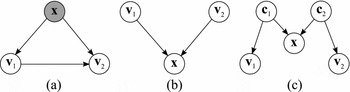
Two simple causal networks with common causes.
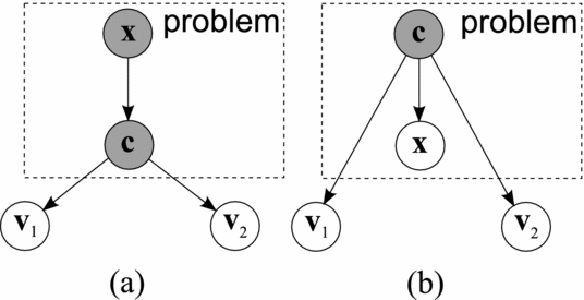
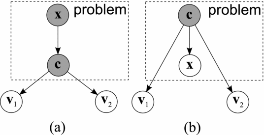
One can represent common causes graphically, as in Figure 1a. Figure 1a is a very simple causal network, depicting the causal relations between a set of variables. A node signifies a phenomenon, mathematically represented as a random variable. An arrow signifies a causal influence in the direction of the arrow.Footnote 11 For simplicity, this and all other figures show only the first two votes, labelled v1 and v2. Both votes are causally influenced by a common cause c (common causes are shown as grey nodes in all figures). If, for instance, the problem is to judge whether a defendant is guilty, then the common cause c in Figure 1a could be a commonly observed witness report, fingerprint, or other shared evidence; in all these examples, c is causally influenced by the fact x of whether the defendant is guilty, as represented by the arrow pointing from x towards c.Footnote 12 The effect of c on votes is indicated by the arrows from c towards each vote. Note that there are no arrows between any votes, indicating that the votes do not have a causal influence on each other. But even though the votes are causally independent, they are not probabilistically independent due to the common cause c.
Compare Figure 1a with 1b. In 1b, the two votes v1 and v2 are still influenced by the common cause, but now the direction of causality between common cause and state is swapped so that c is affecting x. To make this plausible, consider an example. Suppose the task for the voters is to decide whether the streets are wet in Windsor, but all voters are placed in central London. Further suppose that the voters follow a simple heuristic: they predict that the streets are wet in Windsor if and only if the weather is bad in London. In that case, c could be seen as the weather pattern over southeast England, influencing both the votes and the state. So, in this network the common cause c (the weather) influences the state x (dry or wet streets in Windsor), and not the other way round, unlike in Figure 1a.
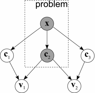
Let us consider a more complicated example. In Figure 2 we include a number of causes from c1 to c3. We can now distinguish between private and common causes. In this causal network, the cause c2 affects both votes and hence is a common cause. c1 and c3, by contrast, are private causes because they only affect one vote each. By definition, common causes are nodes that have directed paths of arrows to more than one vote node. This is why x is also a common cause (and is therefore displayed in grey): it has paths running to v1 (through c1 or c2) and to v2 (through c2 or c3).
A causal network with private and common causes.
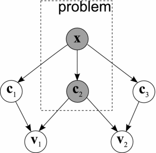
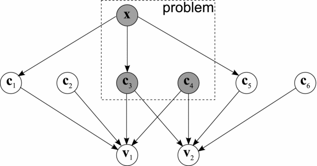
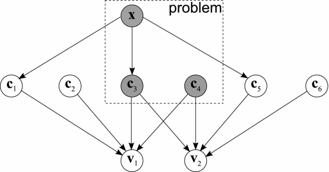
Figure 3 shows another, slightly more complicated, causal network. As before, we have common causes (c3, c4 and x) and private causes (c1, c2, c5 and c6). But in contrast to the previous figures, we can now distinguish between non-evidential causes that are not related to the state (c2, c4 and c6) and evidential causes that are. Non-evidential causes are factors that influence voters causally but do not provide them with evidence as to the correct alternative. These could be common non-evidential causes (such as the weather influencing all our economic advisors in the example above) or private non-evidential causes (such as a domestic argument influencing the judgement of one advisor).
A causal network with private and common causes, some of which are non-evidential.
In all figures shown so far the votes v1 and v2 are not state-conditionally independent because of common causes (other than x). That votes have such common causes is not in any way unusual. To assume that there are none, as the classical CJT does, is to assume a highly construed, artificial decision problem that is unlikely to occur in real-life settings. Thus, Classical Independence is typically violated. This means that the conclusions of the CJT rest on a (typically) false premise. The upshot is that the independence assumption must be revised.
We now introduce a more defensible independence assumption. The CCP implies that events are independent conditional on all their common causes. So independence of votes can be achieved if we conditionalize in the right way. The classical CJT conditionalized on x only. But to catch all the common causes, both evidential and non-evidential, we propose to conditionalize on the decision problem at hand. Following Dietrich (Reference Dietrich2008), the decision problem is a description of all relevant features of the task the group faces. The problem captures not only the state of the world but also all relevant circumstances, which we interpret as all common causes of the votes, thus excluding purely individual factors. We therefore conditionalize on the state of the world and all common causes, as indicated by the dashed rectangles in Figures 1–3. Both components of a decision problem are indispensable. Defining the problem without the circumstances does not work, as we have seen. Defining it without the state x is not plausible either, since this would leave the correct answer indeterminate. Often x is itself a common cause anyhow, as in Figures 1a, 2 and 3 but not in Figure 1b.
We now return to the formal model, leaving the motivational discussion based on causal networks behind. As far as model ingredients are concerned, only one amendment of the classical model is needed. We keep the correct voting events R 1, R 2, . . . but dispose of the state variable x in favour of a new random variable π, the problem, whose realisations are the various possible problems π that the group might face.Footnote 13 Interpretationally, the problem captures not just the state of the world but also the circumstances (common causes) the voters face.
We are now ready to state our revised independence premise.
New Independence. The events R 1, R 2, . . . that voters 1, 2, . . . vote correctly are independent conditional on the problem π.Footnote 14
This assumption is far more defensible than the classical one; by conditionalizing on the problem, we fix all those circumstances which, if left variable, could lead to voter correlation. In Figure 3, for instance, by conditionalizing on the problem one conditionalizes on all the common causes, both evidential (like c3 in Figure 3) and non-evidential (like c4 in Figure 3), so that the two events become probabilistically independent. In the terminology of causal networks, the common causes ‘screen off’ the votes from each other, so that conditionalizing on these causes removes any correlations between votes.
For the interested reader, appendix B briefly sketches the more formal network-theoretic foundation of New Independence; there, the network-theoretic motivation given above is turned into a theorem.
3. THE NEED TO REVISE THE COMPETENCE ASSUMPTION
The Classical Competence assumption is not unreasonable; in fact it is plausibly true. It tells us that the voters are more likely to vote correctly than incorrectly. But when combined with our New Independence assumption (rather than with the unrealistic classical one) it doesn't imply that large groups are better than small ones in their majority judgements.
Consider our group of economic advisers again. It is plausible to assume that each economist is on average better than random in answering economic yes/no questions such as whether a recession is imminent. However, we also know that economists are often not competent when considering one single problem, because some problems are more difficult than others. For instance, very few economists correctly predicted that the initially quite limited banking crisis of 2008 would trigger a major recession in 2009. With hindsight we have learned that predicting this crisis was a difficult problem because economists faced misleading data and worked with questionable or incorrect assumptions. In many other settings, predicting a recession is easy (or at least easier) and economists are more likely to be correct in their predictions. Economists can be competent on average, as demanded by the Classical Competence assumption, without being competent on a difficult problem.
Classical Competence may hold, but since our New Independence assumption conditionalizes on the problem, we will need a problem-specific notion of competence. To show this need we give a stylized example in which large groups are much worse than small ones, despite classical voter competence. This demonstrates that the conclusions of the classical CJT may fail if Classical Independence is replaced with New Independence while retaining Classical Competence. Suppose there are only two types of problems, ‘easy’ and ‘difficult’ ones, where each type is equally likely to occur. Each voter i is correct on any easy problem with probability 0.99, and on any difficult one with probability 0.49. That is,
 \begin{linenomath}\begin{equation*}
\Pr (R_{i}|\pi)=\left\lbrace \begin{array}{l@{\quad}l}0.99 & \mbox{for every easy problem $\pi $}\\0.49 & \mbox{for every difficult problem $\pi $.} \end{array} \ \ \ \ \ \right.
\end{equation*}\end{linenomath}
 \begin{linenomath}\begin{equation*}
\Pr (M_{n})=\frac{1}{2}\times \Pr (M_{n}|\boldsymbol{\pi}\text{is easy})+\frac{1}{2}\times \Pr (M_{n}|\boldsymbol{\pi}\text{is difficult})\text{,}
\end{equation*}\end{linenomath}
 \begin{linenomath}\begin{equation*}
\Pr (M_{n})\approx \left\lbrace \begin{array}{l@{\quad}l}\frac{1}{2}\times 1+\frac{1}{2}\times\frac{1}{2}=\frac{3}{4} & \text{for small}n\\[5pt]
\frac{1}{2}\times 1+\frac{1}{2}\times 0=\frac{1}{2}& \text{for large}n \text{.} \end{array} \ \ \ \ \ \right.
\end{equation*}\end{linenomath}
 $\Pr (R_{i})=\frac{1}{2}\times 0.99+\frac{1}{2} \times 0.49=0.74$. Also the two state-conditional competence parameters, Pr(Ri|x = 1) and Pr(Ri|x = 0), exceed $\frac{1}{2}$ under mild additional conditions (essentially, there shouldn't be a too high correlation between problem type and state). So, Classical Competence holds. Despite the voters' high competence, the majority's competence in a large group is low and well below individual competence. Indeed, the probability that the majority is correct is
where the term Pr(Mn|π is easy) is roughly one, but the term Pr(Mn|π is difficult) is roughly $\frac{1}{2}$ if n is small (because voters are only slightly worse than fair coins) but tends to zero as n tends to infinity;Footnote 15 so,
Large groups are worse here than small groups or single individuals! In terms of our example, asking just one economist would be better than asking many because the majority of the many is increasingly likely to get the difficult problem wrong.
We thus need a new notion of competence: one that is relative to the decision problem. Let us define a voter i’s (problem-specific) competence as  $p_{i}^{\boldsymbol{\pi}}=\Pr (R_{i}|\boldsymbol{\pi})$, the probability that i votes correctly conditional on the problem. Its value depends on the problem; intuitively, it is high for ‘easy’ problems and low for ‘difficult’ ones. In the last example, problem-specific competence is 0.99 or 0.49, depending on whether the problem is easy or difficult. The value taken for a particular problem π – a particular realization of π – is called the competence on π, denoted
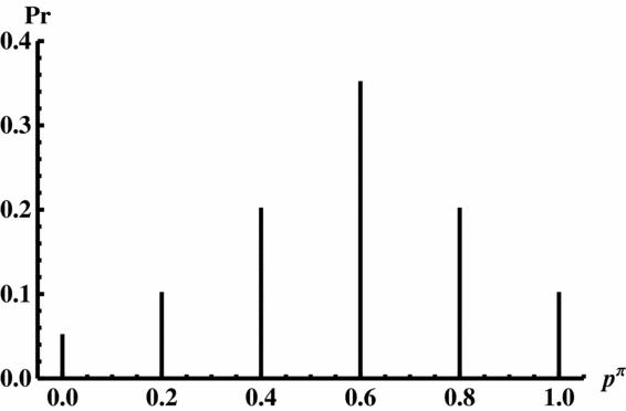
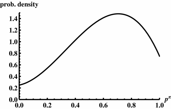
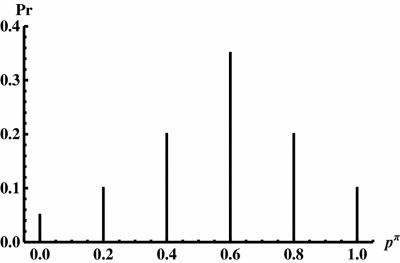
 $p_{i}^{\pi}=\Pr (R_{i}|\pi)$. Figure 4 gives an example of how the distribution of a voter i’s problem-specific competence could look like. There is a 10% probability of facing a problem on which competence is as high as 1 (i.e. the voter is always right), a 20% probability of facing a problem on which competence is 0.8, and so on for the competence levels of 0.6, 0.4, 0.2 and 0. While in Figure 4 problem-specific competence follows a discrete distribution (with six possible values), Figure 5 shows an example in which problem-specific competence follows a continuous distribution given by a density function over the interval [0, 1]. Of course, many other discrete or continuous distributions of problem-specific competence are imaginable.
A discrete distribution of problem-specific competence with tendency to exceed $\frac{1}{2}$. The x-axis shows competence levels, the y-axis their probabilities.
A continuous distribution of problem-specific competence with tendency to exceed $\frac{1}{2}$. The x-axis shows competence levels, the y-axis their probability densities.
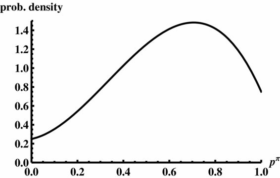
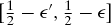
Notice that in Figures 4 and 5 a voter's problem-specific competence on the interval [0, 1] tends to exceed $\frac{1}{2}$, so that, informally, he is more likely to face an ‘easy’ problem (on which competence is high) than a ‘difficult’ problem (on which competence is low). In short, the voter finds more problems easy than difficult. Clearly, this is a notion of voter ‘competence’, but a somewhat different one than that required by Classical Competence. To state this notion more precisely, we first formally define what it means for a (discrete or continuous) random variable or distribution in the interval [0, 1] to tend to exceed $\frac{1}{2}$. In the discrete case (see Figure 4), it simply means that the value $\frac{1}{2}$ + ϵ is at least as probable as the symmetrically opposed value $\frac{1}{2}$ − ϵ, for all ε > 0. In the continuous case with a continuous density function (see Figure 5), it means that this density is at least as high at $\frac{1}{2}$ + ϵ as at $\frac{1}{2}$ − ϵ, for all ε > 0.Footnote 16 (Since all inequalities need only hold weakly this is a weak definition of ‘tendency to exceed $\frac{1}{2}$’; an alternative, strong definition is provided in Appendix A.)
We are now ready to state the new competence assumption:
New Competence. Problem-specific competence  $p_{i}^{\boldsymbol{\pi}}$ (i) tends to exceed $\frac{1}{2}$ and (ii) is the same for all voters i, that is,
 $p_{i}^{\boldsymbol{\pi}}\equiv p^{\boldsymbol{\pi}}$.
To paraphrase this condition once more, the problem is more likely to be of the sort on which voters are competent than of the sort on which they are incompetent (where voters are homogeneous in competence, as in the classical setup). There are many plausible examples where (discrete or continuous) problem-specific competence tends to exceed $\frac{1}{2}$, as in Figures 4 and 5.Footnote 17
The New Competence assumption formalizes an idea stated informally at the beginning of the section in terms of our economist example. The economists face easy and difficult problems. Some problems are very hard, for example predicting the global recession of 2009, but fortunately not all problems are like that. If the economists are good economists they find most problems easy and fewer problems difficult. Unlike the Classical Competence assumption, our new assumption makes no explicit statement about the economists’ average competence across all problems, or across all problems for which a given state x in {0, 1} obtains. Instead, we assume that the economists more often have high than low competence.
As expected, our competence assumption fails for the paradoxical scenario discussed earlier in this section, since there a voter's problem-specific competence is less likely to be 0.51 than 0.49, since Pr(p π = 0.51) = 0 and Pr(p π = 0.49) = $\frac{1}{2}$.Footnote 18 The violation of New Competence is the deeper reason for our counterintuitive finding that large groups are worse than single individuals.
4. A NEW JURY THEOREM
Our New Jury Theorem is based on the New Independence and Competence assumptions. To introduce it, consider again our panel of economic advisers having to predict whether there will be a recession. We assume (from New Independence) that given any problem the events of correct predictions are independent across voters. We also assume (from New Competence) that the prediction problem is more likely to be easy than difficult. Our New Jury Theorem states that increasing the group size will increase the probability of a correct majority, sampled across prediction problems. This is the old non-asymptotic conclusion of the CJT, but based on new premises. Our New Jury Theorem also states that for very large groups the collective competence no longer approaches one (revising the old, unrealistic asymptotic conclusion). Rather, the asymptotic value now depends on the proportion of easy problems.
More precisely, the theorem goes as follows:
New Jury Theorem. Suppose New Independence and New Competence. As the group size increases, the probability that a majority votes correctly (i) increases, and (ii) converges to a value which is less than one if Pr(p π > $\frac{1}{2}$) ≠ 1 (and one if Pr(p π$\frac{1}{2}$) = 1).
Remark: As the proof shows, the value to which the probability of a correct majority converges is
 \begin{linenomath}\begin{equation*}
\Pr \left(p^{\boldsymbol{\pi}}>\frac{1}{2}\right) +\frac{1}{2}\Pr \left(p^{\boldsymbol{\pi}}=\frac{1}{2}\right),
\end{equation*}\end{linenomath}
While proving the non-asymptotic conclusion is not straightforward (see Appendix C), it is easy to develop an intuition of what is driving the asymptotic conclusion and the remark. We know that voters (our economic advisers, for instance) have a probability greater than $\frac{1}{2}$ to vote correctly on easy problems, smaller than $\frac{1}{2}$ on difficult problems, and equal to $\frac{1}{2}$ on boundary problems. So, by the law of large numbers, in the limit the majority will be correct on easy problems, wrong on difficult problems, and correct with probability $\frac{1}{2}$ on boundary problems. Hence, the limiting probability of the majority being correct, averaged over all problems, is as specified in the remark. For example, if our economic advisers face easy problems 80%, difficult problems 20%, and boundary problems 0% of the time, then increasing the group of advisers will let their collective competence converge to 0.8.
The conclusion that majority performance increases crucially depends on the assumption that problem-specific competence tends to exceed $\frac{1}{2}$. We have so far only defined a weak sense of ‘tendency to exceed $\frac{1}{2}$’, while relegating an alternative, strong definition to Appendix A. If in our theorem we use the weak definition, then in the conclusion ‘increases’ means ‘weakly increases’ because of some rare, degenerate cases in which majority performance remains constant.Footnote 19 But if we use the strong definition, then ‘increases’ means ‘strictly increases’. See Appendix A for details.
The mathematical power and generality of our New Jury Theorem is that it holds regardless of how we specify the problem variable π. Indeed, although we have suggested a specific interpretation of π – it captures common causes – we are mathematically free in how we specify it. Let us illustrate this flexibility by considering two very simple specifications, which depart from our suggested interpretation by not capturing the common causes. These ‘naive’ specifications allow us to recover (in fact, strengthen) the classical CJT in two variants. For under these specifications our premises and conclusions reduce to the classical ones.
First, suppose π takes only two values, 0 and 1, representing the state of the world. So π plays precisely the same role as the state in the classical CJT; we accordingly write x for π. To show that we obtain the Classical CJT, note that Classical Independence implies (in fact, is directly equivalent to) New Independence, and Classical Competence implies New Competence, so that our theorem tells us that the probability of a correct majority vote is increasing in group size and (by Pr(px > $\frac{1}{2}$) = 1) converges to one, just as in the Classical CJT. In fact, this strengthens the Classical CJT since New Competence is a weaker premise than Classical Competence.Footnote 20
Second, assume even more simply that π takes only one value – there is just a single problem. Conditionalizing on this fixed problem is as much as not conditionalizing at all. Therefore, our two premises take a particularly simple form:
– the events R 1, R 2, . . . are (unconditionally) independent, and
– competence – the unconditional probability
 $\Pr (R_{i})$ – is at least $\frac{1}{2}$ and the same across voters.

As for our theorem's conclusions, they are here the classical ones: majority competence is increasing in group size and converges to one (unless competence is exactly $\frac{1}{2}$).
5. EPISTEMIC DEMOCRACY: DELIBERATION AND EDUCATION
Our findings have implications for theories of epistemic democracy. This section develops two issues. First, our framework brings to light the benefits of deliberation by removing the worry that independence could be undermined once our new independence notion is adopted. Second, the framework rehabilitates the importance of individual competence for group performance, and hence of education and other competence-boosting policy measures.
Normatively attractive conceptions of democracy involve interactions of voters before the vote. Indeed, many democratic theorists emphasize the importance of deliberation for democratic legitimacy or the quality of democratic outputs. The problem is that such interactions may undermine independence when construed classically, as many have stressed. Nonetheless, confusion prevails over how deliberation creates dependence, and what this implies for jury theorems. Adrian Vermeule describes the challenge well:
What is unclear is whether, and to what extent, independence is compromised by deliberation, discussion, or even common social background or professional training. [. . .] Absent any general account of this, the basic reach of the Jury Theorem is not well understood and no amount of possibility theorems or anecdotes about wise crowds will tell us whether the Theorem is an important tool of political and legal theory or a minor curiosity. (Vermeule Reference Vermeule2009: 6–7, reference and footnote omitted)
Our analysis responds to this challenge by offering the required ‘general account’ – in terms of causal networks – and by revising the independence notion so as to conditionalize on all common causes, including deliberation. A somewhat different response would be to stick to Classical Independence and try to enforce it by preventing all deliberation, as discussed by Grofman and Feld (Reference Grofman and Feld1988) in their seminal work connecting the Condorcet Jury Theorem with Rousseau's ‘general will’. Many find this approach normatively unacceptable. Aside from the normative worry, preventing deliberation is only sensible if it is true that deliberation creates dependence. But is it? Jeremy Waldron is guardedly optimistic that it is not:
The sort of interaction between voters that would compromise independence would be interaction in which voter X decided in favour of a given option just because voter Y did. [. . .] But X's being persuaded by Y in argument or holding itself open to such persuasion does not in itself involve X's deciding to vote one way rather than another because of the way Y is voting. (Waldron in Estlund et al. Reference Estlund, Waldron, Grofman and Feld1989: 1327)
Waldron here identifies the paradigmatic case of dependence: one voter following another blindly. Spelled out in our causal-network-theoretic terms, Waldron's point is that persuasion and deliberation by themselves do not undermine independence because they do not constitute causal effects (arrows) between votes but causal effects (arrows) from earlier phenomena c – such as speech acts – to votes. Thus restated, it becomes clear that Waldron's argument is in fact a defence of New rather than Classical Independence, since persuasive speech acts will, like other common causes of votes, threaten Classical but not New Independence. Indeed, persuasion counts among the more subtle threats to Classical Independence, working through common causation rather than inter-causation of votes, as illustrated in many of our figures above. Persuasion and deliberation could, for instance, mean that the voters align their theories or the set of evidence they use, thereby introducing powerful common causes that undermine Classical Independence.
David Estlund points out that Classical Independence can sometimes be met even when there are common causes or inter-causation of votes (Estlund Reference Estlund2008: 225). He refers to causal setups where the different effects cancel each other out such that probabilistic independence obtains. It needs to be said, however, that while such settings are logically possible, they are exceedingly rare, especially when many voters are involved. Typically, common causes are ubiquitous, and there is little hope that Classical Independence is preserved after deliberation.
However, deliberation does not necessarily increase voter dependence in the classical sense. It could decrease dependence by reducing the influence of certain other common causes (like room temperature) or direct causal influences between voters. It is therefore not always obvious whether deliberation overall increases or decreases dependence, another reason why the classical CJT literature struggles so much with deliberation. Our framework, by contrast, avoids this fruitless struggle. We give the deliberative process its proper place by including it in the description of the problem π, and after having conditionalized on this richly described problem, deliberation does not threaten independence any more.
The classical framework leaves one with the unsatisfactory diagnosis that successful deliberation typically increases voter competence on the one hand, but typically reduces voter independence on the other. Given this unresolved trade-off, the overall effect on group performance could be positive or negative. The diverging claims in the literature about whether deliberation is beneficial demonstrate this all too well. With our New Theorem, by contrast, we can focus exclusively on how deliberation affects (New) Competence. In the language of our framework, deliberation is epistemically beneficial if it increases the voters' problem-specific competence (that is, shifts its distribution to the right). If it does, it also raises the probability that a majority is correct. Thus, deliberation should be interpreted as a process that affects the probability distribution of problem-specific competence, without undermining New Independence. For illustration, consider our economic advisers one last time. If they deliberate and exchange evidence or views, they do not thereby threaten New Independence (because this deliberation process is part of the problem we conditionalize on), but they might raise their problem-specific competence, turning difficult into easier problems. Consequently, a group of deliberating economists may perform better because they are more likely to face decisions they tend to get right, while isolated economists may not.
Our framework has another advantage over the classical one. In its policy recommendation, the classical framework puts all the emphasis on increasing the size of the electorate, suggesting that this suffices for optimal group performance. Classically, large groups can be made infallible without increasing individual competence, just by increasing group size. This loses sight of another important aspect of institutional design: the improvement of individual competence. Our framework restores the picture, showing that individual competence levels matter considerably, since they determine the upper bound on group performance. Policy measures such as improving education may raise the upper bound. Put bluntly, not just the size but also the quality of crowds matters.
6. A NEW JURY THEOREM FOR INTERCHANGEABLE VOTERS
Ladha (Reference Ladha1993) proves a jury theorem based on the assumption that the voters (more precisely, the events that they vote correctly) are interchangeable in de Finetti's sense. Our New Jury Theorem is mathematically related to Ladha's jury theorem for interchangeable voters. In fact, it can be used to derive a more general variant of Ladha's theorem, as we now show.
Intuitively, finitely many events are interchangeable if they are perfectly symmetric in their probabilities. For instance, the probability that only the first event holds equals the probability that only the fourth holds, the probability that only the first and third hold equals the probability that only the second and fifth hold, and so on. Formally, the sequence of correct voting events in the group of size n, (R 1, . . ., Rn), is interchangeable if for any permutation  $(R_{i_{1}}, \ldots,R_{i_{n}})$ and any subgroup J ⊆ {1, . . ., n}, it is equally likely that only the voters in J vote correctly as it is that only the voters in {ij:j ∈ J} vote correctly, i.e.
 \begin{linenomath}\begin{equation*}
\Pr \left(\left(\cap _{i\in J}R_{i}\right)\cap \left(\cap _{i\in \lbrace 1, \ldots,n\rbrace \backslash J}\overline{R_{i}} \right)\right)=\Pr \left(\left(\cap _{i\in J}R_{i_{j}}\right)\cap \left(\cap _{i\in \lbrace 1, \ldots,n\rbrace \backslash J}\overline{R_{i_{j}}}\right)\right)\text{,}
\end{equation*}\end{linenomath}
Ladha makes the following assumption:
Voter Interchangeability. The events of correct voting (R 1, R 2, . . .) are interchangeable.
The assumption of interchangeability can be motivated by interpreting probabilities as representing the beliefs of an observer or social planner with limited information, for whom the voters look perfectly symmetric (no matter whether voters are objectively similar in that way). The mathematical import of voter interchangeability is that, by de Finetti's Theorem (Reference de Finetti1937), it implies the existence of a (discrete or continuous) random variable α in [0, 1], conditional on which these correct voting events (i) are independent and (ii) each have the same probability Pr(Ri|α) = α.
This conditional independence of the correct voting events suggests applying our New Jury Theorem to the case in which the problem π is defined as α (which is mathematically possible, although it deviates from our interpretation of π as capturing common causes). For this specification of the problem π the homogeneity part of New Competence holds since problem-specific competence Pr(Ri|π) (= Pr(Ri|α) = α) is the same for all voters i. In addition, we obtain the peculiar result that problem-specific competence Pr(Ri|π) and the problem π are the same random variable (namely, α), so that problem-specific competence tends to exceed $\frac{1}{2}$ (as assumed in New Competence) just in case π (= α) tends to exceed $\frac{1}{2}$. Hence, our New Jury Theorem can be re-stated as follows for this particular specification of the problem:
Jury Theorem For Interchangeable Voters. Suppose Voter Interchangeability holds and the random variable α obtained in de Finetti's Theorem tends to exceed $\frac{1}{2}$. As the group size increases, the probability that a majority votes correctly (i) increases, and (ii) converges to a value which is less than one if Pr(α > $\frac{1}{2}$) ≠ 1 (and one if Pr(α > $\frac{1}{2}$) = 1).
Conceptually, this theorem operates in a slimmer setup than our earlier theorem because it does not require the exogenous random variable π. Instead, it draws on the random variable α, which is generated endogenously from the assumption of interchangeability. One may interpret α as the degree to which the decision task at hand is ‘easy’, since conditional on α a voter votes correctly with probability α.
The variable α is less obscure than it may seem, since it can be defined directly from the correctness events R 1, R 2, . . . Indeed, α can be obtained as the correctness frequency, i.e. the proportion of correct votes (in the limit as the group size increases). Using this approach to α, one may reformulate our Jury Theorem For Interchangeable Voters without referring to de Finetti's Theorem. Details are given in Appendix A.
Again, the theorem can be read in different ways, depending on whether ‘tendency to exceed $\frac{1}{2}$’ is defined in a weak or strong sense. In the first case the term ‘increases’ in the theorem's conclusion means ‘weakly increases’ (since in rare and degenerate cases majority performance remains constant), while in the second case ‘increases’ means ‘strictly increases’.
How does our theorem generalize Ladha's precursor? Ladha assumes Voter Interchangeability (like us) and assumes that the distribution of α is of a certain kind, which is a special case of our assumption that α tends to exceed $\frac{1}{2}$.Footnote 22 From these assumptions, Ladha deduces that the probability of majority correctness weakly exceeds the probability of single-voter correctness Pr(Ri), which follows from our non-asymptotic conclusion.Footnote 23
Finally, we remark that the value to which the probability of a correct majority converges in the theorem is
 \begin{linenomath}\begin{equation*}
\Pr \left(\boldsymbol{a}>\frac{1}{2}\right) +\frac{1}{2}\Pr \left(\boldsymbol{a}=\frac{1}{2}\right) \text{.}
\end{equation*}\end{linenomath}
7. CONCLUSION
Condorcet's classical jury theorem has an enormous influence, but its independence assumption is implausible and is responsible for the overly optimistic asymptotic conclusion that ‘large groups are infallible’. The non-asymptotic conclusion that ‘larger groups perform better’, by contrast, is often plausible, but is in need of a new justification, grounded on more defensible premises. We have provided such a justification. Our revised independence assumption does not require independence across all decision problems but independence given the specific problem. This allows us to conditionalize on common causes which would otherwise have induced dependence. This new independence assumption requires a new competence assumption: rather than assuming voter competence on average over all problems, we assume that the voters' problem-specific competence is more often high than low. Based on our two revised premises, our New Jury Theorem retains the classical conclusion that ‘larger crowds are wiser’ but obtains the new asymptotic conclusion that ‘large crowds are fallible’. Specifically, the probability of a correct majority vote converges to the probability that the problem is easy in a technical sense. These conclusions vindicate majoritarian democracy – it is worth listening to many rather than few – without being absurdly optimistic about the correctness of democratic decisions. The move from the classical CJT to our New Jury Theorem can be summarized in a table:

Our theorem leads to different policy implications than the classical one with regard to the importance of deliberation and education. The worry that deliberation threatens voter independence disappears by moving to our new notion of independence, so that one can focus on the potentially beneficial effect of deliberation on voter competence. The importance of promoting voter competence (through education, deliberation and other measures) is rehabilitated. Indeed, while the classical model implies that the level of voter competence is essentially irrelevant – since large enough groups are infallible even if their members are just a little competent – our model implies that the performance of large groups strongly depends on voter competence, as measured by the proportion of decision problems voters find easy (in our technical sense). Overall, we believe our findings give more credibility to epistemic arguments for democracy based on jury theorems.
A. SOME EXTENSIONS
First extension. As already mentioned, there are different readings or variants of our New Jury Theorem. They differ, firstly, in the precise definition of when a random variable (here, problem-specific competence) ‘tends to exceed $\frac{1}{2}$’, and secondly, in whether the theorem's conclusion that majority performance increases holds in the weak or strict sense. Only one (weak) notion of ‘tendency to exceed $\frac{1}{2}$’ was defined in the main text; it leads to weakly increasing group performance (though the cases where majority performance increases non-strictly are rare and degenerate; see footnote 19 for examples).
We now introduce two alternative notions of when a random variable or distribution in [0, 1] ‘tends to exceed $\frac{1}{2}$’. (We state the definitions for the discrete case; see footnote 24 for the general case.) Our original (‘first’) notion can be termed ‘weak tendency to exceed $\frac{1}{2}$’ and was defined by the condition that
 \begin{equation}
\begin{array}{c}\text{for all}\epsilon \in (0,\frac{1}{2}]\text{the value}\frac{1}{2} +\epsilon \text{is at least as probable as}\frac{1}{2}-\epsilon . \end{array}
\end{equation}
To obtain the second notion we modify this condition by lifting the requirement about the probabilities of the boundary values 1 and 0. The second notion can be termed ‘weak tendency to exceed $\frac{1}{2}$within the open interval (0, 1)’ and is defined by the following condition (note that ϵ ≠ $\frac{1}{2}$):
 \begin{equation}
\begin{array}{c}\text{for all}\epsilon \in (0,\frac{1}{2})\text{the value}\frac{1}{2} +\epsilon \text{is at least as probable as}\frac{1}{2}-\epsilon . \end{array}
\end{equation}
Finally, to obtain the third notion we further modify the condition by excluding the extreme case that all inequalities are equalities. This third notion can be termed ‘strong tendency to exceed $\frac{1}{2}$ within (0, 1)’ and is defined by the condition thatFootnote 24
 \begin{equation}
\begin{array}{c}\text{for all}\epsilon \in (0,\frac{1}{2})\text{, the value}\frac{1}{2} +\epsilon \text{is at least as probable as}\frac{1}{2}-\epsilon \text{,}\\
\emph {and}\, \text{at least one of these inequalities holds in the strict sense.} \end{array}
\end{equation}
We can now formally state three alternative readings of our New Jury Theorem:
Remark. The New Jury Theorem holds in three variants: we may
(a) use the first notion of ‘tendency to exceed
$\frac{1}{2}$’ and define ‘increasingness’ weakly; or(b) use the second notion of ‘tendency to exceed
$\frac{1}{2}$’ and define ‘increasingness’ weakly; or(c) use the third notion of ‘tendency to exceed
$\frac{1}{2}$’ and define ‘increasingness’ strictly.
Variant (a) of the theorem uses the main text's definition of ‘tendency to exceed $\frac{1}{2}$’. Variant (b) logically strengthens variant (a) by lifting the assumption that problem-specific competence is at least as likely to be 1 than 0. Variant (c) shows that our strong sense of ‘tendency to exceed $\frac{1}{2}$’ allows for the stronger conclusion that group performance grows strictly.
Note that the probabilities with which problem-specific competence takes on any of the boundary values 0 and 1 is irrelevant for the growth of majority performance, and for whether this growth is strict. In short, the boundary values do not matter because conditional on problem-specific competence being 1 (resp. 0) the probability of a correct majority is constant – it equals 1 (resp. 0) regardless of the group size.
Second extension. Our Jury Theorem For Interchangeable Voters also has different readings:
Remark. Our Jury Theorem For Interchangeable Voters holds in each of the variants (a), (b) and (c) of the previous remark.
Note again that whether majority performance grows – and whether it does so strictly – only depends on how the variable α is distributed within (0, 1).
Third extension. The variable α in our Jury Theorem For Interchangeable Voters can be defined as the correctness frequency. The correctness frequency is formally defined as the limit as n→∞ of the proportion of correct votes  $\frac{1}{n}\sum _{i=1}^{n}\chi _{R_{i}}$, where
 $\chi _{R_{i}}$ is the indicator variable of Ri, which is 1 if Ri holds and 0 otherwise. To see why the correctness frequency equals α (except on a zero-probability event), observe that, for every value α of α, it is true that conditional on α = α the correct voting events are independent with equal probabilities Pr(Ri|α) = α, so that by the law of large numbers the correctness frequency
 $\frac{1}{n}\sum _{i=1}^{n}\chi _{R_{i}}$ converges to α with probability one.Footnote 25
This observation about α implies that our Jury Theorem For Interchangeable Voters can be re-stated without invoking de Finetti's Theorem, namely by replacing ‘the random variable α obtained in de Finetti's Theorem’ by ‘the correctness frequency α’. The theorem then states as follows (where the only modified part is put in italics):Footnote 26
Jury Theorem For Interchangeable Voters. Suppose Voter Interchangeability holds and the correctness frequency α tends to exceed $\frac{1}{2}$. As the group size increases, the probability that a majority votes correctly (i) increases, and (ii) converges to a value which is less than one if Pr(α > $\frac{1}{2}$) ≠ 1 (and one if Pr(α > $\frac{1}{2}$) = 1).
B. THE CAUSAL FOUNDATIONS OF NEW INDEPENDENCE
We here introduce causal network terminology more precisely, and give sufficient conditions on causal interconnections for New Independence, citing a result to be proved in a more technical follow-up paper. Mathematically, this appendix is independent of the main text; it uses a different, explicitly network-theoretic model in order to give foundations for New Independence. In this appendix, causal relations are part of the formal setup, and the problem π is not a primitive but is defined as the complex random variable consisting of all common causes of votes plus the state x (if not already a common cause). In this setup, we give a formal justification of New Independence in the form of a theorem which derives, rather than assumes, New Independence, based on plausible conditions on the causal relations, which are met in Figures 1–3 and in many other causal networks.
In a causal network, a variable a is said to be a direct cause of another b (and b a direct effect of a) if there is an arrow pointing from a to b (‘a → b’). Further, a is a cause of b (and b an effect of a) if there is a directed path from a to b, i.e. a sequence of variables starting with a and ending with b such that each of these variables (except from the last one) directly causes the next one. A variable is a common cause (effect) of some variables if it is a cause (effect) of each of them. A variable is a private cause of a vote if it is a cause of this vote but of no other votes.
The following can be proved:
Theorem (informally stated). Suppose the votes v1, v2, . . . and the state x are part of a causal network over these and any number of other random variables, and suppose probabilities are compatible with these causal relations.Footnote 27
(a) If no vote is a cause of any other vote, then the votes are independent conditional on the set
$\mathcal {C}$ of all common causes of some votes;(b) If no vote is a cause of any other vote, and the state x is not a common effect of any votes or private causes thereof,Footnote 28 then the votes are also independent conditional on the augmented set
$\mathcal {C}\cup \lbrace \mathbf {x}\rbrace$ (i.e. New Independence holds with the problem identified with this augmented set).


Many different causal networks, such as those in Figures 1–3, meet the conditions laid out in part (b) of the theorem. In such networks the votes are independent conditional on the problem and New Independence holds. However, some rather special causal setups violate the conditions of part (b), hence of New Independence. We give three elementary examples in Figure 6. Note that votes have no common causes in 6b and 6c, and have just x as a common cause in 6a, so that in all three cases the problem on which we conditionalize consists of x alone. Therefore, New and Classical Independence here reduce to the same condition, so that the figures are in fact counterexamples to both independence conditions. In 6a, vote 1 influences vote 2. With such a direct causal connection between the votes independence is clearly violated. In 6b, the votes cause the state of the world, which is implausible. Such a network could arise if the state of the world (the correct judgement) was simply defined as the majority judgement, but this is incompatible with a procedure-independent notion of correctness as usually assumed in epistemic conceptions of democracy. Again, independence is violated.Footnote 29
Violations of New Independence.

A more complicated case is displayed in Figure 6c. Here the state is the causal product of two different private causes of votes. Independence would require that the votes are independent conditional on the state. But this is not the case, as we can see by considering the following interpretation of causal network 6c. Suppose state x represents the fact of whether parties A and B will form a coalition. Suppose, for simplicity, that A and B will form a coalition if and only if in each party a majority of members supports forming the coalition. c1 represents the fact of whether there is enough support in A, c2 of whether there is enough support in B. Voter 1 is an expert for party A, and bases his prediction entirely on the mood in party A (thus c1’s causal effect on v1), while voter 2 is an expert for party B and bases her prediction only on the mood in B (thus c2’s causal effect on v2). Thus, each voter votes that the coalition takes place just in case he or she thinks there is enough support in the party studied. Imagine we know that the state is, say, that the coalition does not take place. If Independence were true, then voter 1’s vote could not tell us anything about voter 2’s vote. But voter 1’s vote can tell us something: if voter 1 votes, say, for the coalition taking place, then voter 2 probably votes the opposite, because voter 1’s vote indicates that party A is willing, and hence (since the coalition does not take place) that party B refuses to coalesce, which voter 2 will know.
The upshot of this discussion is that our New Independence assumption will hold for most causal setups, but is violated when either there is a direct causal relation between the votes, or the state is itself commonly caused by votes or private causes thereof. This is not only a problem for New Independence – Classical Independence is also violated under such circumstances.
C. PROOF OF OUR NEW JURY THEOREM
We now prove our New Jury Theorem (in all three variants mentioned in appendix A). Two preliminary remarks are due. First, for simplicity we assume that the set of possible problems, to be denoted Π, is countable (with each of its subsets being measurable), and that every problem π ∈ Π occurs with positive probability: Pr(π) > 0. As a result, problem-specific competence has a discrete distribution over [0, 1], supported by a finite set (as in Figure 4) or a countably infinite set. Proofs without this restriction are available on request; they express expectations using (Lebesgue) integrals instead of sums.
Second, some of the summations used below involve an apparently uncountable number of terms (as in ‘∑p∈[0,1] . . .’). Nonetheless these sums are well-defined because the number of non-zero terms is always countable (and because if this number is countably infinite then the sum converges to a value that does not depend on the order of summation).
We now turn to the proof. Suppose New Independence and New Competence hold. The proof proceeds in four steps. Only the last step uses that problem-specific competence tends to exceed $\frac{1}{2}$ (and hence, only that step distinguishes between the three versions of the theorem, i.e. the three possible definitions of ‘tendency to exceed $\frac{1}{2}$’ given in appendix A).
Step 1. Fix any group size n in {1, 3, 5, . . .}. For any problem π ∈ Π consider Pr(Mn|π), the conditional probability that the number of correct votes exceeds  $\frac{n}{2}$ given the problem π. Given the problem π, this number is the sum of n independent Bernoulli variables with parameter p π (by New Independence and New Competence). Hence this number follows a Binomial distribution with parameters n and p π, that is, takes each value m in {0, 1, . . ., n} with probability
 $\frac{n!}{m!(n-m)!}(p^{\pi})^{n}(1-p^{\pi})^{n-m}$, and more generally falls into each set of values
 $S\subseteq \mathbb {R}$ with a probability of
 \begin{linenomath}\begin{equation*}
B_{n,p^{\pi}}(S):=\sum _{m\in \lbrace 0,1, \ldots,n\rbrace \cap S}\frac{n!}{m!(n-m)!}(p^{\pi})^{m}(1-p^{\pi})^{n-m}\text{.}
\end{equation*}\end{linenomath}
 $S=(\frac{n}{2},n]$:
 \begin{linenomath}\begin{equation*}
\Pr (M_{n}|\pi)=B_{n,p^{\pi}}\left(\left(\frac{n}{2},n\right] \right) \text{.}
\end{equation*}\end{linenomath}
 \begin{linenomath}\begin{equation*}
\Pr (M_{n})=\sum _{\pi \in \Pi}\Pr (M_{n}|\pi)\Pr (\pi)=\sum _{\pi \in \Pi}B_{n,p^{\pi}}\left(\left(\frac{n}{2},n\right] \right) \Pr (\pi)\text{.}
\end{equation*}\end{linenomath}
 $\sum _{p\in [0,1]}\sum _{\pi \in \Pi: p^{\pi}=p}$’. Thereby we obtain that
 \begin{eqnarray*}
\Pr (M_{n}) &=&\sum _{p\in [0,1]}B_{n,p}\left(\left(\frac{n}{2},n \right] \right) \sum _{\pi \in \Pi: p^{\pi}=p}\Pr (\pi)\\
&=&\sum _{p\in [0,1]}B_{n,p}\left(\left(\frac{n}{2},n\right] \right) \Pr (p^{\boldsymbol{\pi}}=p)\text{.}
\end{eqnarray*}
$\frac{1}{2}$, respectively. Specifically, S 1 is given by
 \begin{equation}
S_{1}={\displaystyle \sum _{p\in (\frac{1}{2},1]}}B_{n,p}\left(\left(\frac{n}{2},n\right] \right) \Pr (p^{\boldsymbol{\pi}}=p)\text{.}
\end{equation}
 \begin{eqnarray*}
S_{2}& =&{\displaystyle \sum _{p\in [0,\frac{1}{2})}}B_{n,p}\left(\left(\displaystyle\frac{n}{2},n\right] \right) \Pr (p^{\boldsymbol{\pi}}=p)\\
& =&{\displaystyle \sum _{p\in [0,\frac{1}{2})}}\left\lbrace 1-B_{n,p}\left(\left[ 0,\displaystyle\frac{n}{2}\right) \right) \right\rbrace \Pr (p^{\boldsymbol{\pi}}=p)\\
& =&{\displaystyle \sum _{p\in [0,\frac{1}{2})}}\Pr (p^{\boldsymbol{\pi}}=p)-{\displaystyle \sum _{p\in [0,\frac{1}{2})}}B_{n,p}\left(\left[ 0, \displaystyle\frac{n}{2}\right) \right) \Pr (p^{\boldsymbol{\pi}}=p)\text{.}
\end{eqnarray*}
$\frac{1}{2}$), and (ii) another sum which (through a change of variable from p to 1 − p) can be rewritten as
 ${\sum\nolimits_{p\in (\frac{1}{2},1]}}B_{n,1-p}([ 0,\frac{n}{2})) \Pr (p^{\boldsymbol{\pi}}=1-p)$. Here,
 $B_{n,1-p}([ 0,\frac{n}{2}))$ can in turn be rewritten as
 $B_{n,p}((\frac{n}{2},n])$; the reason is that
 \begin{eqnarray*}
B_{n,1-p}\left(\left[ 0,\frac{n}{2}\right) \right) & =&\sum _{m=0, \ldots,\frac{n-1}{2}}\frac{n!}{m!(n-m)!}(1-p)^{m}p^{n-m}\text{and}\\
B_{n,p}\left(\left(\frac{n}{2},n\right] \right) & =&\sum _{m=\frac{n+1}{2}, \ldots,n}\frac{n!}{m!(n-m)!}p^{m}(1-p)^{n-m}\text{,}
\end{eqnarray*}
 \begin{equation}
S_{2}=\Pr \left(p^{\boldsymbol{\pi}}<\frac{1}{2}\right) -{\displaystyle \sum _{p\in (\frac{1}{2},1]}}B_{n,p}\left(\left(\frac{n}{2},n\right] \right) \Pr (p^{\boldsymbol{\pi}}=1-p)\text{.}
\end{equation}
 \begin{linenomath}\begin{equation*}
S_{3}=B_{n,\frac{1}{2}}\left(\left(\frac{n}{2},n\right] \right) \Pr \left(p^{\boldsymbol{\pi}}=\frac{1}{2}\right)\text{.}
\end{equation*}\end{linenomath}
 $B_{n,\frac{1}{2}}((\frac{n}{2},n])$ is, just as
 $B([ 0,\frac{n}{2}))$, equal to $\frac{1}{2}$ because the binomial distribution
 $B_{n,\frac{1}{2}}$ is symmetric around its mean
 $\frac{n}{2}$. So,
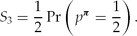 \begin{equation}
S_{3}=\frac{1}{2}\Pr \left(p^{\boldsymbol{\pi}}=\frac{1}{2}\right) \text{.}
\end{equation}
By adding expressions 4, 5 and 6, we obtain that
 \begin{equation}
\Pr (M_{n})=S_{1}+S_{2}+S_{3}={\displaystyle \sum _{p\in (\frac{1}{2},1]}} B_{n,p}\left(\left(\frac{n}{2},n\right] \right) \Delta (p)+\Gamma \text{,}
\end{equation}
 \begin{eqnarray*}
\Delta (p)& =&\Pr (p^{\boldsymbol{\pi}}=p)-\Pr (p^{\boldsymbol{\pi}}=1-p) \text{,}\\
\Gamma & =&\Pr \left(p^{\boldsymbol{\pi}}<\frac{1}{2}\right) +\frac{1}{2} \Pr \left(p^{\boldsymbol{\pi}}=\frac{1}{2}\right) \text{.}
\end{eqnarray*}
Step 2. In this step we show that for fixed  $p\in(\frac{1}{2},1]$ the binomial probability in 7,
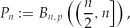 \begin{equation}
P_{n}:=B_{n,p}\left(\left(\frac{n}{2},n\right] \right) \text{,}
\end{equation}
 \begin{equation}
P_{n+2}=P_{n}+(2p-1) \binom{n}{\frac{n+1}{2}}
\left[ p(1-p)\right] ^{\frac{n+1}{2}}\text{.}
\end{equation}
$\frac{1}{2}$ < p ≤ 1, the second term on the right hand side of 9 is non-negative (and positive if p ≠ 1), so that P n+2 ≥ Pn (and P n+2>Pn if p ≠ 1).
While the recursion formula 9 appears in the literature (e.g. Grofman et al. Reference Grofman, Owen and Feld1983), we cannot find a published derivation; let us therefore mention a simple combinatorial argument to its effect. We again conditionalize on a given problem π ∈ Π and write p for the corresponding problem-specific competence p π. Fix any odd group size n (∈{1, 3, . . .}). Recall that P n+2 is the (problem-conditional) probability of the event M n+2 that more than half of the first n + 2 votes is correct. This event can be partitioned into two subevents: the subevent M n+2\Mn that more than half of the first n + 2 but fewer than half of the first n votes are correct, and the subevent M n+2∩Mn that more than half of the first n + 2 and also more than half of the first n votes are correct. We can therefore decompose P n+2 into a sum:
 \begin{linenomath}\begin{equation*}
P_{n+2}=\Pr (M_{n+2}\backslash M_{n}|\pi)+\Pr (M_{n+2}\cap M_{n}|\pi)\text{.}
\end{equation*}\end{linenomath}
 \begin{linenomath}\begin{equation*}
\Pr (M_{n+2}\cap M_{n}|\pi)=\Pr (M_{n}|\pi)-\Pr (M_{n}\backslash M_{n+2}|\pi)=P_{n}-\Pr (M_{n}\backslash M_{n+2}|\pi)\text{,}
\end{equation*}\end{linenomath}
 \begin{equation}
P_{n+2}=P_{n}+\Pr (M_{n+2}\backslash M_{n}|\pi)-\Pr (M_{n}\backslash M_{n+2}|\pi)\text{.}
\end{equation}
 $\frac{n+1}{2}$ of the first n votes (i.e. a narrow majority) must be incorrect – which happens with probability
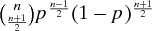 $\binom{n}{\frac{n+1}{2}}p^{\frac{n-1}{2}}(1-p)^{\frac{n+1}{2}}$ – while the next two votes must be correct – which happens with probability p 2. By multiplication we therefore obtain that
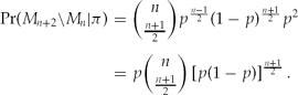 \begin{eqnarray}
\Pr (M_{n+2}\backslash M_{n}|\pi) &=& \binom{n}{\frac{n+1}{2}}
p^{\frac{n-1}{2}}(1-p)^{\frac{n+1}{2}}p^{2} \nonumber\\
&=&p \binom{n}{\frac{n+1}{2}}
\left[ p(1-p)\right] ^{\frac{n+1}{2}}\text{.}
\end{eqnarray}
 $\frac{n+1}{2}$ of the first n votes (i.e. a narrow majority) is correct – which has probability
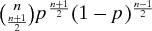 $\binom{n}{\frac{n+1}{2}}p^{\frac{n+1}{2}}(1-p)^{\frac{n-1}{2}}$ – while the next two votes are incorrect – which has probability (1 − p)2. Thus, again by multiplication,
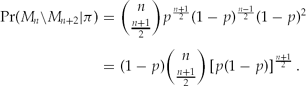 \begin{eqnarray}
\Pr (M_{n}\backslash M_{n+2}|\pi) &=& \binom{n}{\frac{n+1}{2}}
p^{\frac{n+1}{2}}(1-p)^{\frac{n-1}{2}}(1-p)^{2} \nonumber\\
&=&(1-p) \binom{n}{\frac{n+1}{2}}
\left[ p(1-p)\right] ^{\frac{n+1}{2}}\text{.}
\end{eqnarray}
Step 3. We now prove the theorem's asymptotic conclusion. By Step 1 we have to find the limit as n→∞ of the expression 7. We first show that the subexpression  $B_{n,p}((\frac{n}{2},n])$ (=Pn) converges to one as n→∞. Recall that this expression is the probability that the sum of n independent and identically distributed Bernoulli-variables (which are 1 with probability p) belongs to the interval
 $(\frac{n}{2},n]$. Equivalently, it is the probability that
 $\frac{1}{n}$ times this sum belongs to the interval
 $(\frac{1}{2},1]$. This probability converges to 1 as n → ∞, by the law of large numbers and the fact that the interval
 $(\frac{1}{2},1]$ contains the mean p of each Bernoulli-variable.
By 7 and the just-shown fact that  $\lim _{n\rightarrow \infty}B_{n,p}((\frac{n}{2},n])=1$,
 \begin{eqnarray*}
\Pr (M_{n}) &\rightarrow &\sum _{p\in (\frac{1}{2},1]}\Delta (p)+\Gamma\\
&=&\sum _{p\in (\frac{1}{2},1]}\Pr (p^{\boldsymbol{\pi}}=p)-\sum _{p\in (\frac{1}{2},1]}\Pr (p^{\boldsymbol{\pi}}=1-p)+\Gamma\\
&=&\Pr \left(p^{\boldsymbol{\pi}}>\frac{1}{2}\right) -\Pr \left(p^{\boldsymbol{\pi}}>\frac{1}{2}\right) +\Gamma\\
&=&\Pr \left(p^{\boldsymbol{\pi}}>\frac{1}{2}\right) +\frac{1}{2}\Pr \left(p^{\boldsymbol{\pi}}=\frac{1}{2}\right) \text{.}
\end{eqnarray*}
$\frac{1}{2}$) = 1, and less than one otherwise.
Step 4. We finally show the theorem's non-asymptotic conclusion by distinguishing between the three variants of the theorem defined in Appendix A. (Although the first variant follows from the second, we also give a simple direct proof of the first variant.)
Variant (a). Here ‘tendency to exceed $\frac{1}{2}$’ is defined in our first (weak) way. By Step 1 we have to show that expression 7 is weakly increasing in (odd) group size n. This follows from the fact that Γ is a constant in n, Δ(p) is a non-negative constant (by New Competence with the current definition of tendency to exceed $\frac{1}{2}$), and expression 8 is weakly increasing (by Step 2).
Variant (b). Here ‘tendency to exceed $\frac{1}{2}$’ is defined in our second way (i.e. as a weak tendency to exceed $\frac{1}{2}$within (0, 1)). Noting that for p = 1 we have  $B_{n,p}((\frac{n}{2},n]) = 1$, expression 7 for the probability of majority correctness can be re-written as
 \begin{linenomath}\begin{equation*}
\Pr (M_{n})={\displaystyle \sum _{p\in (\frac{1}{2},1)}}B_{n,p}\left(\left(\frac{n}{2},n\right] \right) \Delta (p)+\Delta (1)+\Gamma \text{.}
\end{equation*}\end{linenomath}
 ${\sum _{p\in (\frac{1}{2},1)}}B_{n,p}((\frac{n}{2},n]) \Delta (p)$ is weakly increasing (in odd n). This is the case because for all
 $p\in (\frac{1}{2},1)$, firstly, the coefficient Δ(p) is non-negative (by New Competence with the current notion of ‘tendency to exceed $\frac{1}{2}$’) and, secondly, the coefficient
 $B_{n,p}((\frac{n}{2},n])$ (=Pn) is strictly increasing by Step 2.
Variant (c). Here, ‘tendency to exceed $\frac{1}{2}$’ is defined in our third way (i.e. as a strict tendency to exceed $\frac{1}{2}$within (0, 1)). To show that the probability of majority correctness is now even strictly increasing, we consider again the argument made for variant (b) and add that for some  $p\in (\frac{1}{2},1)$ the coefficient Δ(p) is strictly positive, so that the sum
 ${\sum _{p\in (\frac{1}{2},1)}}B_{n,p}((\frac{n}{2},n]) \Delta (p)$ becomes strictly increasing. ■