2. Bright solitons on top of a hill

2.1. The NLS equation

To study the manipulation of bright solitons in nonlinear media, we will focus on the normal-form PDE for propagation of envelope waves in nonlinear media: the NLS or GP equation [Reference Carretero-González, Frantzeskakis and Kevrekidis13]. The most basic form for this nonlinear PDE in 1D may be cast, after suitable adimensionalization [Reference Carretero-González, Frantzeskakis and Kevrekidis13], as follows:

(2.1)\begin{equation} iu_{t} = -\frac{1}{2}u_{xx} - |u|^2u + V u, \end{equation}

where the complex field $u(x,t)$ represents the wavefunction for the system while the potential $V(x,t)$ may be, in general, a function of space $x$ and time $t$. In actual atomic and optical experiments, the usual observable is $|u|^2$, which corresponds, respectively, to the density of atoms or the optical power. In this work, we fix the sign in front of the (cubic) nonlinear term to be negative, which corresponds to an attractive (focusing) nonlinearity in the realm of BECs (optics). In the absence of external potential effects [ $V(x,t)=0$], the NLS equation (2.1) supports exact bright solitons solutions whose general form is given by:

(2.2)\begin{equation} u(x,t) = A \operatorname{sech}{(A(x-ct-x_0))}\exp{\left(icx+i\frac{A^2-c^2}{2}t\right)}, \end{equation}

where $A$ is the amplitude and (inverse) width of a soliton travelling at constant speed $c$ and initial position $x_0$.

We now focus on the dynamics of bright solitons under the effects of an external potential, which is the combination of a confining parabolic trap and a repulsive hump of the form:

(2.3)\begin{align} V(x,t) &= V_{\rm MT}(x) + V_H(x,t) \\ \notag &= \frac{1}{2}\Omega^2 x^2 + H(t)\operatorname{sech}^{2}(Bx),\end{align}

where $V_{\rm MT}$ correspond to a parabolic confinement of strength $\Omega$ while $V_H$ corresponds to a localized ‘hump’ potential with, in general, time-dependent amplitude $H(t)$ and fixed (inverse) width $B$. In BEC experiments, the parabolic trapping is typically incorporated through the application of a magnetic potential, while the hump potential can be naturally achieved, and precisely controlled, through a blue-detuned external optical (laser) barrier [Reference Helm, Billam and Gardiner23, Reference Wales, Rakonjac, Billam, Helm, Gardiner and Cornish66]. It is also relevant to note that our potential corresponds to a double-well potential that can also be achieved using the competition between a (positive) quartic term and a (negative) quadratic one (see, for instance, Refs. [Reference D’Agosta and Presilla16, Reference Fetter, Jackson and Stringari18, Reference Kalt, Sadaka, Danaila and Hecht25] and references therein). The temporal forcing due to the hump potential will be determined by the following periodic vertical shaking profile:

(2.4)\begin{equation} H(t) = H_0 + \Delta \cos{(\omega t)}, \end{equation}

where the nominal height of the potential hump is denoted by $H_0$, and $\Delta$ and $\omega$ are, respectively, the amplitude and frequency of the periodic shaking off of the nominal height. Note that we will consider a repulsive hump such that $H_0 \gt 0$ and we will try to maintain $\Delta \lt H_0$ so that the hump always presents a repulsive term for the bright soliton.

The main question that this work tackles is whether a soliton sitting on top of the hill can be stabilized under an appropriate periodic forcing (given by $H(t)$) in a manner akin to the stabilization of the forced inverted pendulum, the so-called Kapitza pendulum [Reference Kapitza26, Reference Kapitza27]. In fact, it has been shown that a bright soliton on top of an expulsive parabolic potential can be stabilized by an appropriate periodic variation of the potential strength [Reference Abdullaev and Galimzyanov1] or the strength of the nonlinearity (i.e., the scattering length) [Reference Liang, Zhang and Liu37]. The ultimate mechanism responsible for this stabilization in the (originally, when no vibration is introduced) expulsive potential is the same that in our current work. Namely, after linearization, the resulting dominant dynamical variable (i.e., the position of the soliton) is described by the parametric stability regions of a Mathieu-type ordinary differential equation (ODE). It is also worth mentioning that the Kapitza stabilization mechanism can also be used to stabilize solutions (which are endemically unstable in a homogeneous in space and time setup) through the periodic modulation of the nonlinear term. See, for instance, Ref. [Reference Montesinos, Pérez-García and Michinel45], and references therein, for the stabilization of 2D NLS Townes solitons by an appropriate periodic modulation of the corresponding cubic term.

2.2. Soliton’s statics, stability and eigenmodes

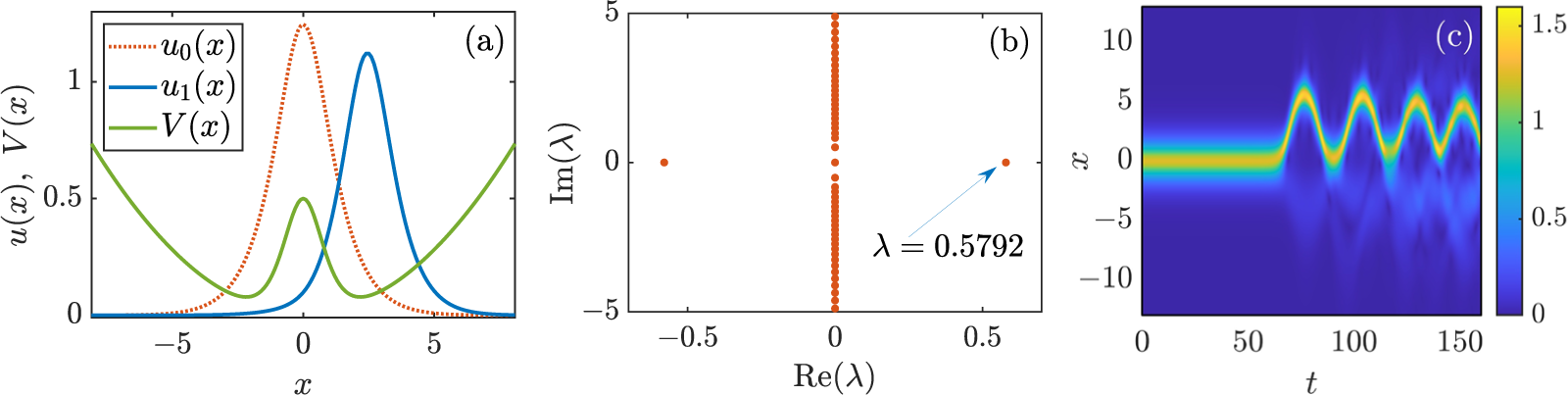
Let us first describe the bright soliton steady states and their stability in the absence of the periodic perturbation, namely when $\Delta=0$. In this static case, the potential (2.3) reduces to the time-independent potential $V(x)=\frac{1}{2}\Omega^2 x^2 + H_0\operatorname{sech}^{2}(Bx)$. As we are considering $H_0 \gt 0$, $V(x)$ corresponds to, for strong enough values of $H_0$, a bistable potential as depicted by the green curve in panel (a) of Fig. 1. The bistability allows for the existence of two solution types: (i) an unstable solution at the top of the hill ( $x=0$) (see dotted red curve in panel (a)) and (ii) a pair of solutions symmetric about $x=0$ (see blue curve in panel (a)). The position of the stable solutions is not of great importance here as we will consider soliton solutions near $x=0$. Nonetheless, it is possible to estimate these stable positions using the VA presented below in Section 3. Stationary solutions are obtained for the steady-state profile $w(x)$ by replacing $u(x,t)=w(x)\exp(-i \mu t)$ in Eq. (2.1) where $\mu$ corresponds to the so-called chemical potential in the context of BECs or the (negative of) the temporal frequency in the context of optics. Steady states are thus solutions of the stationary problem:

\begin{equation*} -\frac{1}{2}w_{xx} - |w|^2w + [V(x)-\mu] w = 0. \end{equation*}

In all numerical results, we employ standard finite difference schemes in space to approximate the second spatial derivatives. Steady states are then numerically found by using standard Newton iterations (see Section 22.2 in Ref. [Reference Carretero-González, Frantzeskakis and Kevrekidis13]), until machine precision is achieved, starting with the analytical solution in the absence of external potential ( $V=0$) given in Eq. (2.2) where $\mu=-A^2/2$ (since $c=0$ in this stationary case). Specifically, for the spatial discretization, we used a second-order central difference scheme on the interval $x\in[-15,15]$ with $N_x=301$ mesh points and (zero) Dirichlet boundary conditions. We checked that finer discretizations did not significantly alter the results. In regards to the time integration for the dynamics, we used a standard fourth order Runge–Kutta method and, in order to ensure numerical stability, we chose the time-step to be half of the threshold time-step given in Ref. [Reference Caplan and Carretero-González11].

Figure 1.

(Colour online) Statics, stability and dynamics for a bright soliton inside the bistable potential consisting of a harmonic trap and a repelling central hump. (a) The potential (green curve), corresponding to $\Delta=0$, $\Omega=0.15$ and $H_0=0.5$, supports unstable  $u_0$ (red dotted curve) and stable  $u_1$ (blue curve) solitons. Both solutions were obtained for $\mu=-1/2$. (b) Stability spectrum for the unstable bright soliton on top of the hill. (c) Typical dynamical destabilization of the soliton on top of the hill when adding a small random perturbation of size $10^{-6}$. Shown is $|u|$ as a function of space-time $(x,t)$.

1 Long description

A line graph with horizontal axis label, x, ranging from negative 7 to 7 with tick labels at negative 5, 0 and 5. The vertical axis label reads, u subscript 0 left parenthesis x right parenthesis comma u subscript 1 left parenthesis x right parenthesis comma V left parenthesis x right parenthesis, ranging from 0 to 1.5 with tick labels at 0, 0.5, 1 and 1.5. A legend lists, u subscript 0 left parenthesis x right parenthesis, u subscript 1 left parenthesis x right parenthesis and minus V left parenthesis x right parenthesis. One dotted curve peaks near x equals 0 at about 1.3 and decreases toward 0 near x equals negative 7 and x equals 7. One solid curve peaks near x equals about 3 at about 1.1 and is near 0 for most other x values. One curve labeled minus V left parenthesis x right parenthesis forms a broad U shape with higher values near x equals negative 7 and x equals 7 at about 0.7, a local rise near x equals 0 at about 0.5 and lower values near x equals about negative 2 and x equals about 2 at about 0.1. The image B showing a scatter plot with horizontal axis label, Re left parenthesis lambda right parenthesis, ranging from negative 0.6 to 0.6 with tick labels at negative 0.5, 0 and 0.5. The vertical axis label reads, Im left parenthesis lambda right parenthesis, ranging from negative 5 to 5 with tick labels at negative 5, 0 and 5. A vertical column of points lies at Re left parenthesis lambda right parenthesis equals 0, extending from Im left parenthesis lambda right parenthesis equals negative 5 to 5. Two isolated points appear near left parenthesis negative 0.5 comma 0 right parenthesis and left parenthesis 0.55 comma 0 right parenthesis. Text inside the plot reads, lambda equals 0.5792. The image C showing a heatmap with horizontal axis label, t, ranging from 0 to 160 with tick labels at 0, 50, 100 and 150. The vertical axis label reads, x, ranging from negative 10 to 10 with tick labels at negative 10, negative 5, 0, 5 and 10. A vertical color scale at the right has tick labels 0, 0.5, 1 and 1.5. A bright band is centered near x equals 0 from t equals 0 to about t equals 70. From about t equals 70 to 160, the bright band follows an oscillating path around x equals 0, with several peaks and troughs between about x equals negative 3 and x equals 3.

Figure 2.

(Colour online) Stability properties for the bright soliton on top of the hill in the absence of the vertical shaking ( $\Delta=0$) and for $\mu=-1/2$. The top row of panels shows the stability eigenvalues associated with the (translational) sliding (see solid curves) and splitting (see dotted curves) modes for two different values of the magnetic trapping strength $\Omega$ as a function of the hump height ( $H_0$). Real and imaginary parts are depicted, respectively, in blue and red. The second row of panels depicts the (c) sliding and (d) splitting eigenmodes (real and imaginary parts depicted, respectively, in blue and red) for $\Omega=0.2$ and $H_0=1.25$ (see, respectively, the cross and plus symbols in panel (b)). The third row of panels depicts the destabilization dynamics after slightly ( $10^{-5}$) perturbing the steady state with the (e) sliding and (f) splitting modes for $\Omega=0.2$ and $H_0=1.25$. The bottom set of panels depicts the two largest instabilities ((g) Re $(\lambda_1)$: sliding and (h) Re $(\lambda_2)$: splitting) in the $(\Omega,H_0)$ plane. Darker colours correspond to less unstable conditions and black corresponds to complete stabilization. The dashed curves depict the theoretical predictions from the effective ODE model as per Eq. (4.4) with (black and white) and without (grey) the soliton height improvement.

Figure 2 Long description

A line plot of lambda subscript 1 comma 2 versus H subscript 0. Horizontal axis label, H subscript 0, with tick labels 0, 0.5, 1, 1.5. Vertical axis label, lambda subscript 1 comma 2, with tick labels minus 1, 0, 1. Units are not indicated. Text reads, a, omega equals 0. Two solid branches and two dotted branches are shown, symmetric about lambda equals 0. The solid branches meet at H subscript 0 equals 0 and separate as H subscript 0 increases. The dotted branches meet on the lambda equals 0 line at an H subscript 0 value between 0.5 and 1, then separate as H subscript 0 increases. The image B showing a line plot of lambda subscript 1 comma 2 versus H subscript 0. Horizontal axis label, H subscript 0, with tick labels 0, 0.5, 1, 1.5. Vertical axis label, lambda subscript 1 comma 2, with tick labels minus 1, 0, 1. Units are not indicated. Text reads, b, omega equals 0.2. Two solid branches and two dotted branches are shown, symmetric about lambda equals 0. The solid branches meet at H subscript 0 equals 0 and separate as H subscript 0 increases. The dotted branches meet on the lambda equals 0 line at an H subscript 0 value between 1 and 1.5, then separate as H subscript 0 increases. Two markers are present: a cross at H subscript 0 between 1 and 1.5 with lambda near 1 and a plus at H subscript 0 between 1 and 1.5 with lambda between 0 and 1. The image C showing a two-curve line plot of W subscript 1 versus x. Horizontal axis label, x, with tick labels minus 5, 0, 5. Vertical axis label, W subscript 1, with tick labels minus 1, 0, 1. Units are not indicated. Label, c. One curve has a minimum near W subscript 1 equals minus 1 at x slightly less than 0 and a maximum near W subscript 1 equals 1 at x slightly greater than 0. The second curve stays closer to W subscript 1 equals 0 with smaller oscillations around x near 0. The image D showing a two-curve line plot of W subscript 2 versus x. Horizontal axis label, x, with tick labels minus 5, 0, 5. Vertical axis label, W subscript 2, with tick labels minus 1, 0, 1. Units are not indicated. Label, d. One curve has a single central peak near W subscript 2 equals 1 at x near 0. The second curve has a smaller central feature near x equals 0 with two side lobes. The image E showing a space time heatmap with axes t and x. Horizontal axis label, t, with tick labels 0, 10, 20, 30, 40, 50. Vertical axis label, x, with tick labels minus 5, 0, 5. Units are not indicated. A color scale bar is labeled 0, 1, 2, with no quantity name shown. Label, e. A bright band begins near x equals 0 for early t and then follows a curved path that reaches x above 5 near t around 25, returns toward x near 0 near t around 30 and rises again to x above 5 near t around 45. The image F showing a space time heatmap with axes t and x. Horizontal axis label, t, with tick labels 0, 10, 20, 30, 40, 50. Vertical axis label, x, with tick labels minus 5, 0, 5. Units are not indicated. A color scale bar is labeled 0, 1, 2, with no quantity name shown. Label, f. A bright band near x equals 0 persists until about t around 20, then splits into two bands that move symmetrically toward positive x and negative x, reaching about x near plus 5 and x near minus 5 around t around 30 to 35, then the bands approach each other and cross near x equals 0 around t around 40. The image G showing a parameter space heatmap with omega on the horizontal axis and H subscript 0 on the vertical axis. Horizontal axis label, omega, with tick labels 0, 0.2, 0.4, 0.6, 0.8, 1. Vertical axis label, H subscript 0, with tick labels 0, 0.5, 1. Units are not indicated. A color scale bar is labeled 0, 0.2, 0.4, 0.6, 0.8, 1, with no quantity name shown. Label, g. Two overlaid boundary curves are present, one dashed and one solid, both rising from near omega equals 0 and H subscript 0 equals 0 toward higher H subscript 0 as omega increases. The image H showing a parameter space heatmap with omega on the horizontal axis and H subscript 0 on the vertical axis. Horizontal axis label, omega, with tick labels 0, 0.2, 0.4, 0.6, 0.8, 1. Vertical axis label, H subscript 0, with tick labels 0, 0.5, 1. Units are not indicated. A color scale bar is labeled 0, 0.1, 0.2, 0.3, 0.4, 0.5, with no quantity name shown. Label, h. Most of the heatmap is near the lowest color scale value, with a localized region of higher values near omega between 0 and 0.2 and H subscript 0 between about 0.8 and 1. Across the figure, omega and H subscript 0 are the repeated parameters. The lambda subscript 1 comma 2 plots show solid and dotted branches that meet on the lambda equals 0 line at different H subscript 0 values for omega equals 0 and omega equals 0.2. The space time heatmaps show one case with a single band that moves in x over t and another case where the band splits into two symmetric branches and later crosses near x equals 0.

As concerns the stability of stationary ( $\Delta=0$) bright solitons at the top of the hill ( $x=0$), we cast the linear perturbation off of the steady state $w(x)$ using the ansatz $ u(x,t)=\left[w(x) + \epsilon\, p(x,t)\right]e^{-i\mu t}$ with perturbation $p(x,t) = a(x)e^{\lambda t}+b(x)e^{\lambda^* t}$ and corresponding eigenvalue $\lambda$ and eigenfunction ${\cal W}=(a,b^*)^T$ where the asterisk denotes complex conjugate and $(\cdot)^T$ denotes the transpose. This linear perturbation yields the so-called Bogoliubov–de-Gennes (BdG) equations, namely the eigenvalue problem (see Chapter 22.2 in Ref. [Reference Carretero-González, Frantzeskakis and Kevrekidis13] for more details):

\begin{align*} iM {\cal W}= i\left(\begin{array}{ccc} M_{11}~ & M_{12} \\[1.0ex] M_{21}~ & M_{22} \end{array}\right) {\cal W} =\lambda {\cal W}, \end{align*}

where the matrix operator $M$ is composed by the blocks:

\begin{align*} M_{11}= \frac{1}{2}\partial_{xx} - \left(2g|w|^2 + V-\mu \right), \quad M_{12}=-g\,w^2, \quad M_{22}=-M_{11}^*, \quad M_{21}=-M_{12}^*. \end{align*}

To numerically compute the stability spectra, we again recur to standard second-order finite differences in space to cast the continuum BdG problem into its discrete counterpart. Panel (b) in Fig. 1 shows a typical example of the stability spectrum for the soliton on top of the hill for a relatively weak hump height. In this case, the system admits a single eigenvalue pair of unstable eigenvalues that corresponds to the instability of the translational mode. This translational mode, or sliding mode as we call it from now on, is responsible for the destabilization of the soliton that eventually slides down the hill as shown in panel (c) of Fig. 1. As we will explain now, it should be noted that, for larger hump heights, there exist another pair of unstable eigenvalues corresponding to the splitting mode of the soliton responsible for ‘rupturing’ the soliton into two equal packets on each side of the hump.

We now systematically extract the most unstable eigenvalues for the soliton on top of the hill as the system parameters are varied. Specifically, we fix 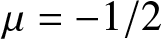$\mu=-1/2$ (corresponding to a soliton of height $A=1$ in the absence of any potential effects) and vary the harmonic trap strength $\Omega$ and the hump height $H_0$. The corresponding results are depicted in Fig. 2. The top panels correspond to the variation of the sliding (solid curves) and splitting (dotted curves) mode eigenvalues as a function of the hump strength in the absence (see panel (a)) and in the presence (see panel (b)) of the parabolic trapping. As it can be seen from this stability spectra, in the absence of the magnetic trap ( $\Omega=0$), the sliding mode becomes unstable (its real part (solid blue curve)) as soon as the hump potential is turned on. Then, for a larger value of the hump strength, a secondary bifurcation is responsible for the splitting mode (dotted curve) to become unstable. In contrast, when the magnetic trap is turned on ( $\Omega \gt 0$), there is a region for relatively small values of the hump height where the sliding mode is stable. Then, for larger values of the hump height, the sliding mode becomes unstable and, for even larger hump heights, the splitting mode also becomes unstable. The overall qualitative effect of the magnetic trap is to ‘shift’ the spectrum to the right and to widen the stability regions as the trap is stronger. Panels (c) and (d) depict, respectively, the sliding and splitting modes for $\Omega=0.2$ and $H_0=1.25$ (see the black cross and plus symbols in panel (b) depicting their respective (unstable) eigenvalues). Panels (e) and (f) show how these unstable modes manifest themselves in the dynamics of the destabilization of the soliton on top of the hill. For the sliding mode (see panel (e)), the instability eventually forces the soliton to slide down the hump and then perform oscillations about the potential minimum. Note that due to radiation effects (see visible lighter blue areas about the main soliton path in yellow), the soliton does have enough energy to come back to its original starting location ( $x=0$). On the other hand, when the soliton is perturbed by the unstable splitting mode, it eventually destabilizes by breaking into two symmetric blobs that slide down over each side of the hump. After their initial sliding, the two blobs perform oscillation and regroup back close to $x=0$ but, again due to radiation loss, the initial condition on top of the hill is not fully recovered. Finally, we depict in panels (g) and (h) the dependence of the destabilization rates (i.e., real part of the eigenvalues) for, respectively, the sliding and splitting modes as a function of the trap strength $\Omega$ and the hump height $H_0$ (black regions correspond to stable choices for the parameters). Note that for all combinations of ( $\Omega, H_0$), the sliding mode is always dominant. Thus, unless one carefully crafts an initial condition that only perturbs along the splitting mode without affecting the sliding mode (precisely as it was done in panel (f)), a typical (random) perturbation will generically destabilize along the sliding mode. This is important in what follows as we are aiming to stabilize the soliton on top of the hill with a periodic perturbation of the hump height in a manner akin to the inverted pendulum. Therefore, we need to primarily focus on taming this sliding mode if we have any hope of achieving such stabilization. As we will see below, in the regions of stabilization of the sliding mode, we were not able to detect destabilization due to the splitting mode and, therefore, we will be able to fully stabilize the soliton on top of the hill.

3. Dynamical reduction of the soliton’s dynamics

Let us now deploy a reduced model that, not only qualitatively but also quantitatively (in appropriate parameter regions), reproduces the dynamics of the bright soliton as it slides along the hump potential. For that purpose, we deploy the VA formalism [Reference Malomed40] (see also Chapter 25 in Ref. [Reference Carretero-González, Frantzeskakis and Kevrekidis13] and references therein). As a preliminary disclaimer, we are going to cast the simplest possible reduced model by using the least amount of variational parameters that can still capture (qualitatively and quantitatively) the statics, dynamics and stability of the soliton under the periodic forcing exerted by the vertically vibrating hump. Nonetheless, we will check that our results do give qualitative and, more importantly, quantitative information about the parameter combinations that allow for the full stabilization of the bright soliton on top of the hill thanks to the effect of the periodic perturbation of the hump’s height.

Proceeding with the standard VA formalism, the NLS (2.1) can be cast by extremizing the action of the Lagrangian density given by:

(3.1)\begin{equation} \mathcal{L}[u] = \frac{i}{2} ( u^{*} u_t - u u_t^{*} ) - \frac{1}{2} |u_x|^2 - \frac{1}{2} |u|^4 - V(x,t) |u|^2. \end{equation}

We then restrict our attention to the following bright soliton ansatz:

(3.2)\begin{equation} u_a(x,t)=A\text{sech}(A(x - \xi(t)))\exp(iv(t)x), \end{equation}

where $A$ is the fixed amplitude and (inverse) width of the soliton while $\xi(t)$ and $v(t)$ are the variational parameters corresponding, respectively, to the position and velocity of the soliton. It is important to stress that we are fixing the soliton amplitude and (inverse) width (namely, they are not variational parameters), and the only variational parameters are the position and velocity of the soliton. Then, using the external potential as the combination of the confining parabolic and the repelling hump potential of Eq. (2.3), it is possible to evaluate the Lagrangian density (3.1) on the soliton ansatz (3.2) and integrate all over space to obtain the effective Lagrangian:

\begin{align*} \mathcal{L}_a =& \int_{-\infty}^{\infty} \mathcal{L}[u_a(x,t)] \, dx \\ =& -\frac{2A^2}{B}\dot{v}(t)\,\xi(t) -\frac{A^2B}{3} - \frac{A^2}{B} v(t)^2 +\frac{2A^4}{3B} - \frac{A^2\Omega^2\left(12B^2\xi(t)^2 + \pi^2\right)}{12B^3} - I(x,t), \end{align*}

where $I(x,t)$ is the overlapping integral between the hump potential and the soliton shape:

(3.3)\begin{equation} I(x,t)\equiv\int_{-\infty}^{+\infty} V_H\,|u_a|^2\, dx =A^2 H(t)\int_{-\infty}^{+\infty} \operatorname{sech}^2(Bx)\operatorname{sech}^2(A(x-\xi))\, dx. \end{equation}

Unfortunately, close form expressions for $I(x,t)$ are only available when the soliton width ( $A$) and the hump width ( $B$) are equal. It should be noted that, in principle, the approach for $A\not=B$ would still hold as the overlapping integral could be, in the general case, numerically integrated. Nonetheless, for the sake of simplicity, we will use from now on the special case $A=B$. In this case ( $A=B$), the overlapping integral yields the close form:

(3.4)\begin{equation} I(x,t)=4H(t)B \operatorname{csch}(B \xi)^2 [B\xi\coth(B\xi)-1]. \end{equation}

Now, proceeding with the VA methodology, we deploy the Euler–Lagrange equation for the variational parameters $\xi(t)$ and $v(t)=\dot\xi(t)$:

\begin{equation*} \frac{d}{dt}\left[\frac{\partial {\cal L}_a}{dv}\right] =\frac{\partial {\cal L}_a}{d\xi}, \end{equation*}

which yields the following effective Newton-type ODE for the soliton position:

(3.5)\begin{equation} \ddot{\xi}= -\frac{d}{d\xi}\left[ V^{\rm eff}(\xi)\right], \end{equation}

where the effective potential is given by

(3.6)\begin{equation} V^{\rm eff}(\xi) = V^{\rm eff}_{\rm MT}(\xi) + V^{\rm eff}_H(\xi) = \frac{1}{2} \Omega^2 \xi^2 + 2H\operatorname{csch}(B\xi)^2[B\xi\coth(B\xi)-1], \end{equation}

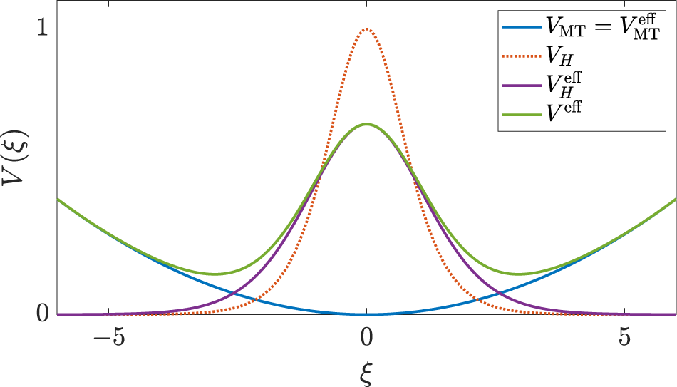
containing, respectively, the effective contributions of the magnetic trap and the hump potential. Note that, contrary to the effective contribution of the magnetic trap that is identical to the original magnetic trap potential, the contribution of the hump towards the effective potential has a similar shape, but is not identical, to the hump potential itself. Figure 3 depicts the different contributions to the original potentials and their effective counterparts.

Figure 3.

(Colour online) The different contributions to the original potentials and their corresponding effective counterparts. See the legend for the description of each contribution. The parameters here correspond to $\Omega=0.15$, $H=1$, $B=1$ and $C=B$.

Figure 4.

(Colour online) Phase space for a soliton inside a combination of harmonic trapping and a repulsive hump for $\Omega=0.15$, $H_0=0.05$ and $B=1$. The light orange, green and purple dots depict the reconstruction of orbits from the PDE numerics, while the thin red and blue curves depict the corresponding orbits for the reduced ODE approach. Panel (a) corresponds to the effective potential (3.6), while panel (b) corresponds to the improved effective potential (3.7). Panel (c) depicts the amplitude of the soliton for the green and purple orbits in panels (a) and (b) by least-squares fitting of a sech profile. The green and purple horizontal lines depict the respective amplitude averages along the orbit, while the black horizontal line corresponds to the estimate soliton height of $A+H_0$. Panels (d) and (e) depict, respectively, the green and purple orbits together with their approximation using the effective ODE models (red: original effective potential (3.6), blue: improved effective potential (3.7).

Figure 4 Long description

A line plot of xi versus zeta with multiple closed orbits. The horizontal axis label is zeta with tick labels minus 1, 0, 1. The vertical axis label is xi with tick labels minus 0.1, minus 0.05, 0, 0.05, 0.1. The plotted curves form nested loops around two centers near zeta about minus 1 and zeta about 1, with several curves crossing at zeta equals 0 and xi equals 0 to form an X shaped intersection. A line plot of xi versus zeta with multiple closed orbits, using the same axis labels and tick labels as image. The plotted curves form nested loops around two centers near zeta about minus 1 and zeta about 1, with several curves crossing at zeta equals 0 and xi equals 0 to form an X shaped intersection. A time series line graph of A versus t. The horizontal axis label is t with tick labels 200, 300, 400, 500. The vertical axis label is A with tick labels 1.04, 1.05, 1.06, 1.07. Two oscillating lines are shown, one varying between about 1.04 and about 1.07 and the other varying between about 1.04 and about 1.05. Three horizontal reference lines are shown at about 1.043, 1.05 and 1.055. A time series line graph of xi versus t. The horizontal axis label is t with tick labels 0, 100, 200, 300. The vertical axis label is xi with tick labels minus 1, 0, 1. Two sinusoidal lines closely overlap, with peaks near xi about 1.3 and troughs near xi about minus 1.3. Peaks occur near t about 20, 100, 180, 260 and 300, with troughs near t about 60, 140, 220 and 290. A time series line graph of xi versus t. The horizontal axis label is t with tick labels 0, 100, 200, 300. The vertical axis label is xi with tick labels 0, 0.5, 1. Three lines are shown. One thick oscillating band stays between about 0.5 and about 0.85. One sinusoidal line oscillates between about 0.45 and about 0.85. One sinusoidal line oscillates between about 0.2 and about 0.8.

Let us now validate the fidelity of the effective ODE reduction to reproduce the bright soliton dynamics in the original PDE model. For this, let us compare the corresponding orbits in phase space $(\xi,\dot\xi)$ for typical parameter values. For the NLS model, we generate bright soliton orbits by using initial conditions starting on the unstable and stable steady states $w(x)$ boosted with a velocity ‘kick’ $v_0$ according to $u(x,0)=w(x)\, e^{i v_0 x}$. The resulting phase space reconstruction for the original NLS model is depicted by the thick light-coloured dots/curves in panel (a) of Fig. 4. For orbits inside the separatrix (separating oscillating orbits on one side of the hump and orbits oscillating across the hump), we boost the stable steady state at the right of the hump and outside the separatrix we boost the unstable steady state centred at $x=0$. The corresponding effective ODE orbits are depicted by the thin red lines. As we can observe from panel (a), the reduced model offers a good qualitative description of the original NLS model; however, it fails at the quantitative level. After further investigation, it becomes evident that the lack of a better (quantitative) match can be accounted for by the fact of the simplicity in the soliton ansatz that we chose to use in the VA approach. In particular, we note that the shape of the phase space orbits is highly sensitive to the amplitude of the soliton. Therefore, to obtain a better quantitative match when using the reduced effective ODE model, it is essential to include more freedom on the soliton amplitude. A direct, albeit more lengthy, approach would rely in casting a VA approach with an ansatz that also includes the soliton amplitude and its chirp as variational parameters (see Section 25.2.1 in Ref. [Reference Carretero-González, Frantzeskakis and Kevrekidis13]). However, to keep our approach as simple and clean as possible and to streamline our presentation, we opt to modify our effective ODE model by introducing the amplitude of the soliton ( $A$) as follows. To keep the overlapping integral (3.3) in closed form as in Eq. (3.4), we will assume that the (inverse) widths of the soliton and the hump are kept constant and equal to each other. Then, a posteriori, we adjust only the amplitude parameter by modifying the strength of the effective potential by a prefactor given by the actual soliton amplitude from the original system. To account for the soliton height, we could extract the average height of the soliton from the original NLS simulations (see panel (c) in Fig. 4). Despite this option giving the best possible match of the effective reduced model (see Appendix A), we opt here for a completely analytical approach. Thus, we approximate the soliton height by $A+H_0$ since, as a first approximation, the height of the soliton on top of the hump will be increased by the height of the hump ( $H_0$) itself. Thus, we simply use same shape for the effective hump potential with a prefactor $(A+H_0)/A$:

(3.7)\begin{equation} \widetilde{V}^{\rm eff}_H(\xi) = \frac{A+H_0}{A} V^{\rm eff}_H(\xi). \end{equation}

This improved effective model allows for (small) variations of the soliton height from the hump width $B$. Panel (b) in Fig. 4 shows how this improved effective model (see thin blue curves) is able to more accurately capture the phase space of the original NLS model. It is important to mention that, since we are going to be studying the stability of the soliton on top of the hill under periodic perturbations, we will be exclusively interested in the approximation of the effective model close to the origin ( $x\approx 0$). The phase space in panel (b) evidences that the improved reduced model is quite accurate in the region $x\approx 0$. Therefore, unless stated otherwise, we will use from now on this improved potential for our effective ODE model of choice. Panel (c) depicts the soliton amplitude for two typical NLS orbits showing that an overall soliton amplitude approximation of $A+H_0$ is a good compromise. Finally, we depict in panels (d) and (e) representative orbits for the original NLS model and both effective models.

4. Stabilization on top of the hill: The Mathieu equation

Now that we have cast an accurate reduced model for the static hump potential, let us consider the case when the vertical shaking is on ( $\Delta \gt 0$). In this case, our improved reduced effective model takes the form of the Newton-type equation (3.5) with the effective potential:

(4.1)\begin{equation} V^{\rm eff}(\xi) = V^{\rm eff}_{\rm MT}(\xi) + \widetilde{V}^{\rm eff}_H(\xi) = \frac{1}{2} \Omega^2 \xi^2 + \frac{A+H_0}{A} 2H(t)\operatorname{csch}(B\xi)^2[B\xi\coth(B\xi)-1], \end{equation}

where $H(t)$ given in Eq. (2.4). As we are interested in the stability of the soliton on top of the hill, for linear stability purposes, it suffices to linearize the ensuing effective equations about $\xi=0$, which yields:

(4.2)\begin{equation} \ddot{\xi}(t)-\left[\left( \tilde{A}\frac{8B^2}{15} H_0 -\Omega^2\right) +\tilde{A}\frac{8B^2}{15} \Delta \cos(\omega t) \right]\xi(t)=0, \end{equation}

where $\tilde{A}\equiv(A+H_0)/A$ as argued before. Equation (4.2) has precisely the form of the Mathieu equation. Indeed, after defining $h\equiv\tilde{A}\frac{8B^2}{15\omega^2}H_0-\frac{\Omega^2}{\omega^2}$, $\delta\equiv\tilde{A}\frac{8B^2}{15\omega^2}\Delta$, and rescaling time according to $\tau\equiv\omega t$, Eq. (4.2) reads:

(4.3)\begin{equation} \frac{d^2 \xi(\tau)}{d\tau^2}-\left[h+\delta\cos(\tau)\right]\,\xi(\tau)=0, \end{equation}

corresponding to the standard form of the Mathieu equation.

The Mathieu equation is a prototypical ODE with periodic coefficients, which is front and centre in the theory of parametric excitation, Floquet stability and resonance tongues [Reference Mathieu41, Reference McLachlan43, 50]. Its importance relies on the fact that many physical systems, very much like the present one, reduce to a Mathieu-type equation after linearization around an equilibrium when a periodic variation of one (or more) parameter(s) is introduced. The Kapitza (or inverted) pendulum is a classic example of this paradigm. In particular, when the pivoting point of a pendulum is vertically driven under the right conditions, the effective periodically modulated gravitational term gives rise, after linearization, to the celebrated Mathieu equation where the stability of the inverted equilibrium can be interpreted through the stability diagram (or stability tongues) of the Mathieu equation [Reference Kapitza26, Reference Landau and Lifshitz35, 50]. The Kapitza pendulum provides a concrete mechanical realization of the broader mathematical phenomenon described by Mathieu and Hill equations where the effects of the periodic parametric forcing can either destabilize or stabilize motion depending on the drive amplitude and frequency [Reference Magnus and Winkler39, Reference McLachlan43, Reference Nayfeh and Mook49]. It is precisely this space of periodic forcing parameters that we will now explore in connection with our physical system consisting of a soliton on top of and oscillating hill. As we mentioned before, the stabilization of the bright soliton on top of the hill is tantamount to the work of Refs [Reference Abdullaev and Galimzyanov1, Reference Liang, Zhang and Liu37] where solitons were stabilized on top of an expulsive parabolic trap by introducing an appropriate periodic variations of, respectively, the trap strength and the strength of the nonlinearity.

Before we use the results from the Mathieu equation, it is worth exploring the stability properties in the case when the vertical shaking is absent ( $\Delta=0$). In that case, the above linear analysis directly predicts the stability threshold from the competition of the stabilizing effects of the parabolic trap and the destabilization deriving from the hump. From the linearized Eq. (4.2) with $\Delta=0$, this threshold directly reads as:

(4.4)\begin{equation} \Omega^{\rm crit} = \sqrt{\frac{8\tilde{A}B^2}{15} H_0}. \end{equation}

This predicts that, in the static case, if $\Omega \lt \Omega^{\rm crit}$ the steady state for $\xi=0$ becomes unstable. Note that we write the above threshold in terms of $\Omega^{\rm crit}$ rather than $H_0^{\rm crit}$ since the adjusted height $\tilde{A}$ depends on $H_0$. At any rate, the threshold (4.4) can be interpreted (i.e., inverted) in practice as a threshold for the hump height such that if $H_0 \gt H_0^{\rm crit}$ the soliton on top of the static hill becomes unstable. We overlayed this threshold prediction for the soliton on top of the hill on the stability diagram of panel (g) in Fig. 2 where we used the soliton height with ( $\tilde{A}=(A+H_0)/A$; see black and white dashed curve) and without ( $\tilde{A}=A$; see grey dashed curve) the soliton height improvement. As it is evidenced from this figure, the improved reduced model with the adjusted soliton height is essential to obtain a good quantitative match between the original NLS model and its ODE reduction.

Figure 5.

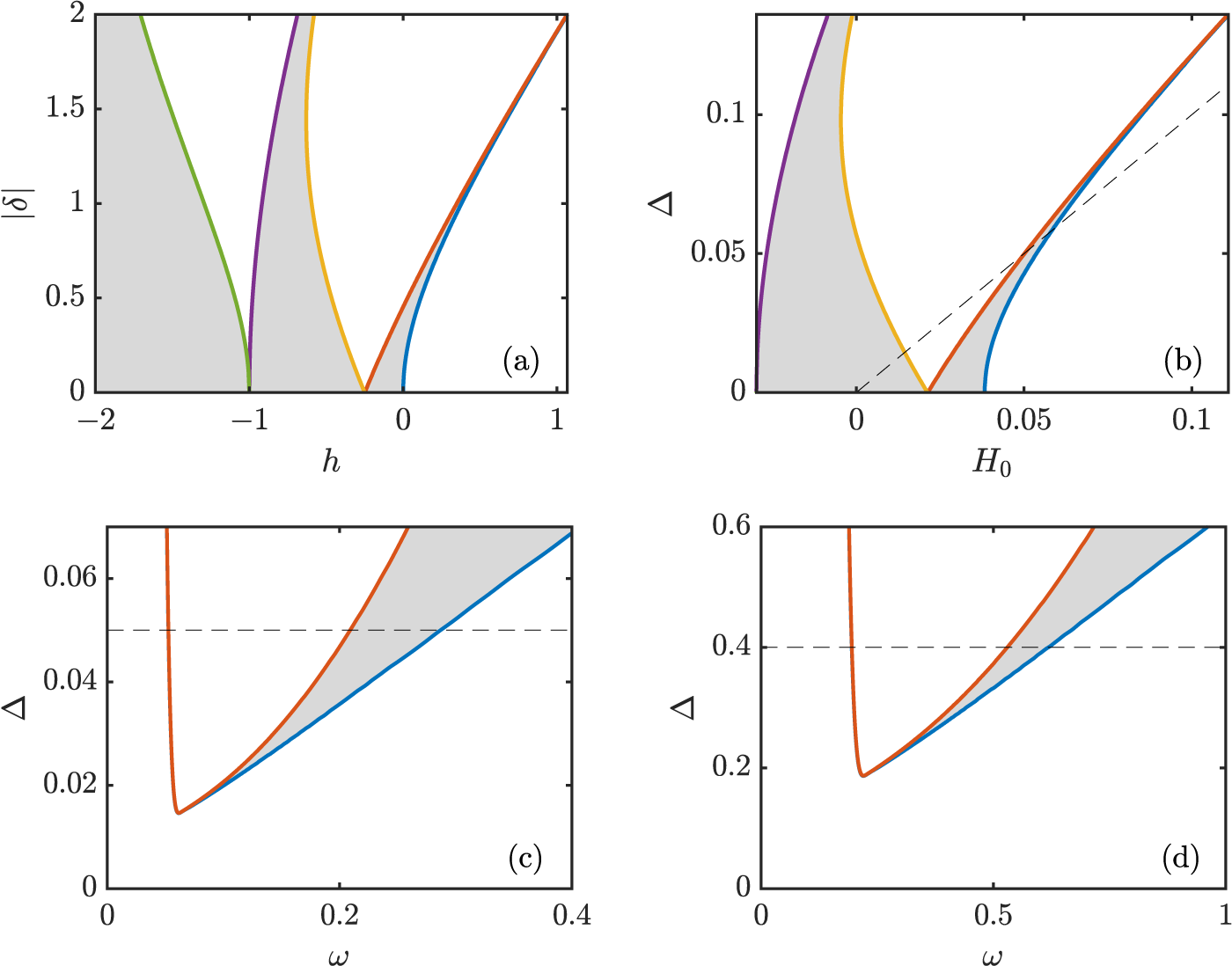
(Colour online) Stability regions (see grey shaded areas) for the Mathieu equation. (a) Mathieu stability regions for Eq. (4.3) as a function of $h$ and $\delta$. (b) Stability regions in the $(H_0,\Delta)$ plane for $(\Omega,\omega,\tilde{A})=(0.15,0.2,A=1)$. (c) and (d) Stability regions in the $(\omega,\Delta)$ plane for $(\Omega,H_0,\tilde{A})=(0.15,0.05,A\!=\!1)$ and $(\Omega,H_0,\tilde{A})=(0.4 ,0.4 ,A\!=\!1)$, respectively. In all the panels, below the dashed line, the periodic forcing potential never takes negative values (i.e., $H_0 \lt \Delta$).

Figure 5 Long description

Four plots illustrating stability regions for the Mathieu equation. Each plot shows shaded areas representing stability under different parameter conditions. Plot (a) displays stability regions as a function of h and vertical bars delta vertical bars. The x-axis is labeled h, ranging from minus 2 to 1 and the y-axis is labeled vertical bars delta vertical bars, ranging from 0 to 2. Stability occurs in shaded regions bounded by curves, with key points at h equals minus 1 and h equals 0 where the boundary touches vertical bars delta vertical bars equals 0. Plot (b) shows stability regions in the H subscript 0 and delta plane. The x-axis is labeled H subscript 0, ranging from 0 to 0.1 and the y-axis is labeled delta, ranging from 0 to 0.1. A dashed diagonal line indicates a reference condition, with stability regions below this line. Plot (c) presents stability regions in the omega and delta plane. The x-axis is labeled omega, ranging from 0 to 0.4 and the y-axis is labeled delta, ranging from 0 to 0.06. Stability is shown between two curves, with a horizontal dashed line at delta equals 0.05 marking a threshold. Plot (d) also depicts stability in the omega and delta plane, with the x-axis labeled omega, ranging from 0 to 1 and the y-axis is labeled delta, ranging from 0 to 0.6. Stability is indicated between two curves, with a horizontal dashed line at delta equals 0.4. The plots illustrate how changes in parameters like h, H subscript 0 and omega affect stability, with shaded regions indicating stable conditions. The curves represent boundaries of stability and the dashed lines serve as reference thresholds.

When the periodic forcing is present ( $\delta \gt 0$), the Mathieu equation is well-known to exhibit stability tongues [Reference Butikov10, Reference Kovacic, Rand and Sah34, Reference Rand56] corresponding to parameter combinations where the orbit starting at $\xi=0$ is completely stable. Panel (a) of Fig. 5 depicts the corresponding main stability tongues in $(h,\delta)$ space. Note that the tongues are symmetric with respect to sign changes in $\delta$. Also note that for our system of interest $\delta$ is always positive while $h$ can be either sign depending on the combination of the system parameters. Let us now map the Mathieu stability tongues onto the original parameters of our bright soliton model under the influence of the parabolic trap and the hump’s periodic vertical shaking. Panel (b) of Fig. 5 depicts such stability tongues as a function of the hump nominal height $H_0$ and shaking amplitude $\Delta$ for the choice $(\Omega,\omega)=(0.15,0.2)$ and without using the bright soliton amplitude improvement (i.e., $\tilde{A}=A$). On the other hand, panels (c) and (d) of Fig. 5 depict the main stability tongue as a function of the periodic shaking frequency $\omega$ and amplitude $\Delta$ for, respectively, $(\Omega,H_0,\tilde{A})=(0.15,0.05,A\!=\!1)$ and $(\Omega,H_0,\tilde{A})=(0.4 ,0.4 ,A\!=\!1)$ (namely, without the soliton height adjustment; we will introduce the height adjustment in the results below). Note that part of the second stability tongue does exist but it happens for large values of $\Delta$ where the hump potential is most of the time negative (i.e., attracting towards $\xi=0$ for the bright soliton). In fact, to stress the fact that we want to showcase stabilization despite having a repelling hump (in the stationary case), we have drawn the dashed lines in Fig. 5. We are precisely interested in the regions below these lines, which correspond to cases where the potential hump is never negative (i.e., it is always repelling).

Figure 6.

(Colour online) Stability diagram of the sliding mode for a bright soliton on top of the hill under a periodic perturbation of frequency $\omega$ and amplitude $\Delta$ with $H_0=0.05$ and $\Omega=0.15$. Depicted is the real part of the most unstable (sliding) eigenvalue of the Floquet spectrum for the calculated periodic orbits. Darker colours correspond to less unstable conditions and black corresponds to complete stabilization. The points A ( $\omega=0.12$) and B ( $\omega=0.36$) correspond to two unstable cases, while the point C ( $\omega=0.19$) corresponds to a stable case; all for $\Delta=0.045$. The grey dashed curves depict the stability boundary regions predicted by the Mathieu equation for the original soliton amplitude of $A=1$, while the black and white dashed curves correspond to the boundary regions for the improved reduced model with $A=1+H_0$.

Figure 6 Long description

The heatmap illustrates a stability diagram with the vertical axis labeled delta from 0 to 0.07 and the horizontal axis labeled omega from 0 to 0.4. The color bar on the right ranges from 0 to 0.1, representing stability levels, with darker shades indicating less unstable conditions and black indicating complete stabilization. Points A and B mark unstable cases, while point C marks a stable case. The diagram shows a stability region where delta is between 0.03 and 0.05 and omega is around 0.15, with transitions occurring as omega increases. The gray dashed curves depict predicted stability boundaries, while black and white dashed curves show improved model boundaries.

Now that we have access to the predictions for the parameter regions where the bright soliton would be stable according to our linear stability analysis of the reduced ODE model, we can now search for stable regions for the original NLS model. To do so, we use parameter values in the window displayed in panel (c) of Fig. 5. For each parameter combination, we then compute the stability spectrum using Floquet theory as follows. We first, for each parameter combination, compute the steady state when the vertical shaking is absent ( $\Delta=0$) using standard fixed-point Newton iterations (as we did in Section 2.2). We then use this steady-state solution as an initial seed for the fixed-point iteration scheme on the map generated, after one period of the forcing, on the norm of the solution. Namely, we find solutions to $|u(x,0)|=|u(x,T)|$ where $T=2\pi/\omega$ is the corresponding forcing period. Subsequently, in order to use the full (complex) solution in the Floquet stability analysis, we extract the phase $\phi$ such that $u(x,0)=u(x,T)\,e^{i\phi}$. In this manner, we obtain numerically the corresponding periodic orbit and its relative phase for each parameter combination. Once we obtain the periodic orbit with a prescribed precision (residuals below $10^{-6}$), we deploy numerically a standard linear stability Floquet analysis [Reference Fairgrieve and Jepson17, Reference Seydel62, Reference Wu, Xia and Xu67] (after factoring out the relative phase $\phi$) to extract the linear stability spectrum for each periodic orbit. Figure 6 displays the largest real part of the Floquet spectrum for $H_0=0.05$ and $\Omega=0.15$ together with the Mathieu stability tongue boundaries from our dynamical reduction. Note that complete stabilization of the original NLS bright soliton on top of the oscillating hump is indeed possible (see region in black). The predicted stability region boundaries obtained through our reductive approach are depicted, for the case without using the soliton height improvement (i.e., $\tilde{A}=A=1$), by the grey dashed curves. As it could have been expected, these predicted boundary regions match qualitatively the actual stability regions but fail to give a good quantitative match. In contrast, when using the effective hump potential with the improved soliton height $\tilde{A}=(A+H_0)/A$, the theoretical prediction (see black and white dashed curves) performs significantly better and allows for a decent quantitative match of the stability region.

Figure 7.

(Colour online) Evolution of the bright soliton under different periodic perturbations. The initial condition corresponds to the computed periodic orbit perturbed by an initial velocity ‘kick’ imparted by multiplying the initial wave by $\exp(i v_0 x)$ with $v_0=10^{-10}$. Panels (a), (b) and (c) correspond, respectively, to the points A, B and C depicted in Fig. 6. Panels (a) and (b) correspond to unstable orbits where the bright soliton rapidly slides down from the top of the hill. In contrast, panel (c) depicts a case inside the stabilization window. In this case, the bright soliton stays on top of the hill indefinitely until the vertical shaking is removed at $t/T=45$ (see vertical dashed line) and, hence, the soliton rapidly slides down from the top of the hill. The panels depict the absolute value of the field as a function of time (scaled by the corresponding shaking period $T=2\pi/\omega$) and space.

Figure 7 Long description

Label, a. No title text is visible above the heatmap. No legend, color key, or scale is visible and no text states what the intensity represents. The horizontal axis label is t over T, with tick labels 0, 2, 4, 6. The vertical axis label is n, with tick labels minus 4, minus 2, 0, 2, 4. A narrow horizontal band is centered around n equals 0 across most of the time range. A localized zigzag shaped feature appears between t over T about 5 and 6, spanning values around n equals 0. Label, b. No title text is visible above the heatmap. No legend, color key, or scale is visible and no text states what the intensity represents. The horizontal axis label is t over T, with tick labels 0, 2, 4, 6, 8, 10, 12, 14. The vertical axis label is n, with tick labels minus 4, minus 2, 0, 2, 4. A narrow horizontal band is centered around n equals 0 across the full time range. The band shifts slightly downward around t over T about 13 to 14. Label, c. No title text is visible above the heatmap. No legend, color key, or scale is visible and no text states what the intensity represents. The horizontal axis label is t over T, with tick labels 0, 5, 10, 15, 20, 25, 30, 35, 40, 45, 50. The vertical axis label is H, with tick labels minus 4, minus 2, 0, 2, 4. A narrow horizontal band is centered around H equals 0 across the full time range. A vertical dashed line is drawn at about t over T equals 45. A localized zigzag shaped feature appears close to t over T equals 50, spanning values around H equals 0.

To showcase the success of stabilizing the soliton on top of the hill via the periodic vertical shaking, we display typical dynamical scenarios inside and outside of the stability region. Figure 7 depicts the three different cases shown by the labelled purple crosses in Fig. 6 after the numerically computed periodic orbit is slightly perturbed by a velocity ‘kick’ (boost) of $10^{-10}$. These correspond to: unstable cases to (A) the left and to (B) the right of the stability region and (C) inside the stability region, which are displayed, respectively, in panels (a), (b) and (c) in Fig. 7. Note that, despite the fact that we used a very small velocity boost of $10^{-10}$, both unstable cases destabilize rather quickly and the soliton slides down the hill after a handful of forcing periods. Also note that the destabilization for case A is faster than the one in case B as the corresponding instability (real part of the stability eigenvalue) is stronger for the former. In contrast, when choosing a parameter combination inside the stable region, the soliton is able to balance on top of the hill for long times (we have checked that it stay stable for thousands of periods; results not shown here). In fact, to showcase more vividly the stabilizing effect of the periodic shaking, for the stable case depicted panel (c) in Fig. 7, we stop the forcing after 45 periods and the bright soliton quickly slides down the hill.

Figure 8.

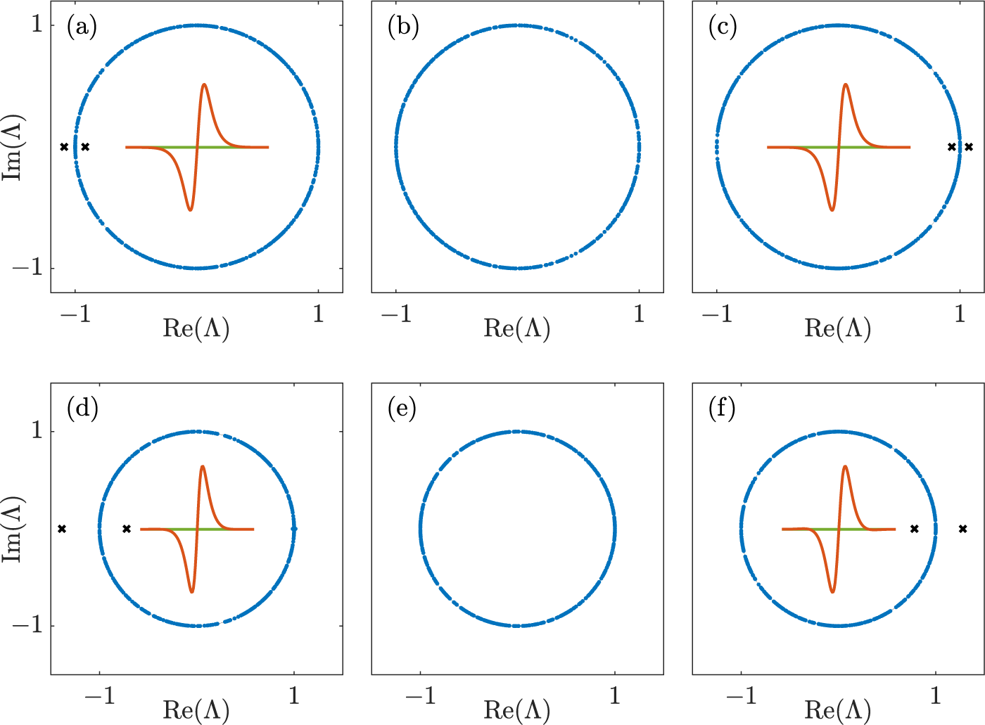
(Colour online) Floquet stability spectra of the periodic orbits corresponding to the points A, B, C, D, E and F depicted in Figs. 6 and 9 (corresponding orbits depicted in Figs. 7 and 10). Non-neutral eigenpairs ( $|\Lambda|\not=1$) are depicted by the black crosses, while neutral ones are depicted by small blue dots. The insets show (in case of instability) the eigenvector associated with the most unstable mode (red and green depict, respectively, the real and imaginary parts). Note that the unstable modes correspond to translational modes, which are responsible of destabilizing the bright soliton from the top of the hill.

Figure 8 Long description

Floquet stability spectra for periodic orbits labeled A to F. Each plot has the x-axis labeled Re open parenthesis capital lambda close parenthesis and the y-axis labeled Im open parenthesis capital lambda close parenthesis, both ranging from minus 1 to 1. Most eigenvalues, shown as small dots, lie on the unit circle, indicating neutral stability. Black crosses represent non-neutral eigenpairs, indicating instability. Insets display eigenvectors associated with the most unstable mode, with red and green lines showing real and imaginary parts. In plot A, crosses appear on the negative real axis. Plot B shows only the unit circle distribution. Plot C has crosses on the positive real axis. Plot D features crosses on the negative real axis. Plot E shows only the unit circle distribution. Plot F has crosses on the positive real axis. The insets suggest translational modes causing instability in certain plots.

In order to shed some light into the instability mechanism, we depict in Fig. 8 the Floquet spectra corresponding to the ensuing dynamical scenarios depicted in Fig. 7 (and the ones depicted in Fig. 10; see below). Note that the Floquet eigenvalues $\Lambda$ are related to the stability eigenvalues $\lambda$ (see Section 2.2) by the relation $\Lambda=e^{\lambda/T}$ where $T$ is the period of the orbit. Floquet eigenvalues $\Lambda$ lying on the unit circle ( $|\Lambda|=1$) correspond to (linearly) neutrally stable modes (depicted by small blue dots), i.e., Re $(\lambda)$=0. Due to the Hamiltonian nature of the underlying PDE of the NLS model, the eigenvalues must appear in pairs (in case of being purely real or purely imaginary) or quartets (in case of being genuinely complex). The modes responsible for the stability or instability of the bright soliton correspond to point-spectrum eigenvalues that will lie off of the unit circle (depicted by black crosses). As it can be noticed from Fig. 8, the instabilities, when present, correspond to real eigenvalues indicating an exponential instability (in contrast with an oscillatory instability). This is straightforward to understand as when the soliton starts sliding down due to the instability, it will continue sliding down on the same side of the hill. We also depict in the insets the eigenmodes associated with the instability, when present, that clearly indicate that the instability is associated with the translational mode, i.e., the sliding down of the soliton from the top of the hill.

Figure 9.

(Colour online) Same meaning and layout as Fig. 6 but for stronger periodic forcing and $H_0=0.4$. The points D ( $\omega=0.475$) and E ( $\omega=0.588$) correspond to two unstable cases while the point F ( $\omega=0.548$) corresponds to a stable case; all for $\Delta=0.490$.

Figure 9 Long description

A heatmap with a horizontal axis labeled omega and tick labels 0.5, 0.55 and 0.6. The vertical axis is labeled Delta with tick labels 0.44, 0.45, 0.46, 0.47, 0.48, 0.49 and 0.5. A vertical scale bar at the right has tick labels 0, 0.1, 0.2, 0.3 and 0.4, indicating the heatmap cell values range from 0 to 0.4. A dashed curve runs from near omega about 0.47 and Delta about 0.5, down to a low point near omega about 0.49 and Delta about 0.46, then rises toward omega about 0.55 and Delta about 0.5. A narrow diagonal band of lower heatmap values follows an increasing relationship between omega and Delta, starting near omega about 0.47 and Delta about 0.44 and extending toward omega about 0.56 and Delta about 0.5. Outside this band, the heatmap shows higher values over much of the remaining omega and Delta range. Three labeled markers are present. D is near omega about 0.48 and Delta about 0.49. F is near omega about 0.55 and Delta about 0.49. E is near omega about 0.59 and Delta about 0.49. D and F lie close to the dashed curve and F lies on or near the diagonal low value band, while E lies away from the diagonal low value band.

Figure 10.

(Colour online) Same meaning and layout as Fig. 7 but for stronger forcing oscillations. Panels (a), (b) and (c) correspond, respectively, to the points D, E and F depicted in Fig. 9. Panels (a) and (b) correspond to unstable orbits where the bright soliton rapidly slides down from the top of the hill. In contrast, panel (c) depicts a case inside the stabilization window. In this case, the bright soliton stays on top of the hill indefinitely until the periodic forcing is removed at $t/T=45$ (see vertical dashed line).

Figure 10 Long description

Three heatmaps display z versus t over T. The horizontal axis is labeled t over T and the vertical axis is labeled z. A color gradient from darker to brighter indicates intensity, with brighter regions representing higher values. The shared feature across all panels is a persistent narrow band centered near z equals 0. The image A shows localized peaks forming a curved feature between t over T equals 3 and 5. The image B shows a similar curved feature between t over T equals 6 and 8. The image C shows a stabilization window with a dashed vertical line at t over T equals 45, after which the band becomes more spread with multiple bright regions. The gradient scale ranges from 0 to 4, representing intensity levels.

Figure 11.

(Colour online) Competition of unstable modes for the periodic solution corresponding to $H_0=0.4$, $\Delta=0.5$, $\Omega=0.4$ and $\omega=0.74$. Panel (a) depicts the Floquet spectrum, while panels (b) and (c) show the eigenfunctions of the two most unstable modes (see, respectively, the cross and plus symbols in panel (a)): (b) sliding mode and (c) splitting mode (real and imaginary parts depicted, respectively, in red and green). Panels (d) and (e) show the dynamical evolution of the unstable periodic solution slightly perturbed by, respectively, the sliding and splitting modes.

Figure 11 Long description

Panel (a) shows a complex-plane scatter plot of eigenvalues. The horizontal axis is labeled Re open parenthesis lambda close parenthesis and the vertical axis is labeled Im open parenthesis lambda close parenthesis. Most points form a near-circle centered at the origin, representing the unit circle, with a few real outliers marked beyond the circle. Panel (b) displays a line plot of V subscript 1 versus x. The horizontal axis is labeled x and the vertical axis is labeled V subscript 1. The baseline curve is constant at zero, while the signal curve dips to a trough near minus 1 around x equals 0, peaks near 1 around x equals 2 and returns toward zero. Panel (c) shows a line plot of V subscript 2 versus x. The horizontal axis is labeled x and the vertical axis is labeled V subscript 2. The baseline curve is constant at zero, while the signal curve peaks near 1 around x equals 0, with small dips on either side. Panel (d) presents a heatmap of x versus time, showing a bright ridge near x equals 0 that shifts to negative x values and later curves to positive x values. Panel (e) displays a heatmap of x versus normalized time t slash T, showing bright regions near x equals 0 at multiple time points. Loop-shaped structures form from t slash T equals 2.5 to 5. Variables include lambda as eigenvalues, V subscript 1 and V subscript 2 as potential profiles, x as spatial coordinate and t slash T as normalized time. The plots illustrate the dynamics of unstable modes, with the spectrum mostly on the unit circle and real outliers, V subscript 1 showing a strong dip then peak, V subscript 2 showing a central peak with side dips and heatmaps showing ridge drift and loop formation.

Next, to showcase that the stabilization mechanism is not exclusive for small hump potentials, we depict in Fig. 9 the stability region for larger hump strengths. As the figure suggests, the stability region for larger hump strengths is greatly reduced when compared to the corresponding one for smaller hump strengths (see Fig. 6). Nonetheless, as evidenced from the Floquet spectra shown in panels (d)–(f) of Fig. 8 and their corresponding dynamical evolutions shown in Fig. 10, it is indeed possible to find completely stable cases in this larger hump strength scenarios. We also note that the prediction using the improved reduced model with the adjusted soliton height (see dashed curves in the figure) is able to predict to a great extent the region of stability.

Finally, as it was the case when the periodic forcing was absent, in the general case with non-zero periodic forcing, the splitting mode might still be present. For instance, we show in Fig. 11 the Floquet spectrum (panel (a)) and it associated unstable eigenmode (panels (b) and (c)) for a case containing an unstable splitting mode. As we can observe, the Floquet spectrum exhibits, in addition to the dominant translational (sliding) mode (see panel (b)), a splitting mode (see panel (c)). Albeit this splitting mode being less unstable that the dominant sliding mode, it is possible to excite it by perturbing the numerically computed periodic orbit with the corresponding eigenmode. Panels (d) and (e) show the ensuing dynamics when perturbing the periodic orbit by, respectively, the sliding and splitting modes. As one may observe, both modes destabilize rather quickly (after a couple of oscillations of the periodic orbit). It would be interesting to find parameter combinations that would switch the dominance between the sliding and the splitting mode. This might be possible as the stabilization provided by the periodic forcing is only designed to tame the sliding mode. Thus, it is conceivable that, for larger values of the hump strength, one would be able to completely stabilize the sliding mode (or at least make it less unstable than the splitting mode) such that the soliton on top of the hill destabilizes along the splitting mode instead of along the sliding one. Searching for such a case falls outside of the scope of the current work.