1. Introduction
Turbulent thermal convection is an important phenomenon that plays a key role in understanding the heat transport and dynamics of several natural and engineering flows (Siggia Reference Siggia1994). One important mechanism that induces turbulent thermal convection is the Rayleigh–Taylor (RT) instability (Boffetta & Mazzino Reference Boffetta and Mazzino2017). The RT instability is a buoyancy-induced hydrodynamic (HD) instability that occurs at the interface between colder (denser) and hotter (lighter) fluids when the hotter fluid supports the colder one in the presence of a gravitational field or when the hotter fluid is accelerated into the colder one (Rayleigh Reference Rayleigh1882; Taylor Reference Taylor1950). In the presence of a magnetic field, the RT instability is known as magnetic RT instability (Bucciantini et al. Reference Bucciantini, Amato, Bandiera, Blondin and Del Zanna2004), which plays an important role in engineering applications and astrophysical phenomena. One of its engineering applications is in the inertial confinement fusion (ICF) (Zhou et al. Reference Zhou, Sadler and Hurricane2024) implosions in which the interactions between the self-generated (Zhang et al. Reference Zhang, Li, Xin, Yan, Wan, Zhang and Zheng2022; Walsh & Clark Reference Walsh and Clark2023) or applied (Walsh Reference Walsh2022) magnetic fields and RT instability can affect the hot spot’s temperature and the target’s thermal losses. Therefore, magnetohydrodynamic (MHD) effects should be considered while designing the ICF devices (Walsh & Clark Reference Walsh and Clark2021). For efficient fusion in ICF devices (Zhou Reference Zhou2017a ), a controlled mixing of the hot and cold fluid is desirable. Therefore, suppression of the RT instability may be achieved by rotating the spherical target as suggested by Tao et al. (Reference Tao, He, Ye and Busse2013). In astrophysical systems, the magnetic RT instability is crucial in the filamentary structures of the Crab nebula (remnant of a supernova explosion) (Hester et al. Reference Hester1996), type-Ia supernovae (Cabot & Cook Reference Cabot and Cook2006; Hristov et al. Reference Hristov, Collins, Hoeflich, Weatherford and Diamond2018), young supernova remnants (Jun & Norman Reference Jun and Norman1996; Abarzhi et al. Reference Abarzhi, Bhowmick, Naveh, Pandian, Swisher, Stellingwerf and Arnett2019), pulsar wind nebulae in expanding supernova remnants (Bucciantini et al. Reference Bucciantini, Amato, Bandiera, Blondin and Del Zanna2004), and quiescent (Ryutova et al. Reference Ryutova, Berger, Frank, Tarbell and Title2010) and solar (Hillier Reference Hillier2017) prominences. Along with the magnetic fields, rotational motions (such as steller, solar and planetary rotations) are also present in many astrophysical settings that can simultaneously influence RT instability and turbulence. For example, accretion through RT instability at the disc-magnetosphere interface depends on the stellar rotation rates and magnetic fields (Kulkarni & Romanova Reference Kulkarni and Romanova2008). The rotation of the Sun causes prominences related to magnetic RT instability to rotate around and be present on the solar disk (Ryutova et al. Reference Ryutova, Berger, Frank, Tarbell and Title2010; Hillier Reference Hillier2017).
The RT instability arises at the slightly perturbed interface between two unequal-density fluids subjected to an acceleration in a direction opposite to the mean density gradient such that the denser (or colder) fluid is pushed and accelerated by the lighter (or hotter) one (Rayleigh Reference Rayleigh1882; Taylor Reference Taylor1950). The instability is triggered when there is a misalignment of pressure (
 $p$
) and density (
 $\rho$
) gradients such that
 $\nabla p \cdot \nabla \rho \lt 0$
, where the pressure gradient results from the acceleration. This misalignment results in the generation of baroclinic torque (
 $\sim \nabla p \times \nabla \rho$
) at the perturbed interface that in turn creates vorticity (
 $\boldsymbol {\omega }$
) and induces a velocity field (
 $\boldsymbol {u}$
), as described by the two-dimensional (2-D) vorticity equation (Kundu et al. Reference Kundu, Cohen and Dowling2015; Roberts & Jacobs Reference Roberts and Jacobs2016)
 \begin{equation} \frac {D \boldsymbol {\omega }}{Dt}=\underbrace {\frac {1}{\rho ^2} \left ( \nabla p \times \nabla \rho \right )}_{\displaystyle \mathrm {Baroclinic\, torque}}, \end{equation}
where
 $\boldsymbol {\omega } = \nabla \times \boldsymbol {u}$
. This results in increased misalignment of the gradient vectors and baroclinic torque. Note that for the thermal convection problem, the density differences reflect temperature fluctuations in the RT configuration. At the initial linear stage, for initial multi-mode perturbations, the short-wavelength (
 $\lambda$
) perturbations (or larger wavenumber
 $k\,(=2\pi /\lambda )$
) grow more rapidly (exponentially) than the long-wavelength perturbations (smaller
 $k$
) according to the growth rate
 \begin{equation} \sigma =\sqrt {kg\frac {\rho _2-\rho _1}{\rho _2+\rho _1}}, \end{equation}
as predicted by the linear stability analysis (Taylor Reference Taylor1950; Chandrasekhar Reference Chandrasekhar1968; Sharp Reference Sharp1984; Youngs Reference Youngs1984) in the absence of surface tension, viscous and diffusive effects, magnetic field and rotation. Here
 $\rho _1$
is the density of the light fluid and
 $\rho _2$
is the density of the heavy fluid. As the perturbation amplitude reaches a size of the order of approximately
 $0.5\lambda$
, the linear phase breaks down and the nonlinear effects emerge in the next stage. The exponential growth rate of short-wavelength perturbations slows down. In contrast, the long-wavelength perturbations grow more rapidly, resulting in the appearance of larger fluid structures of ‘spikes’ of heavy fluid growing into light fluid and ‘bubbles’ of light fluid growing into heavy fluid. As the spikes grow, the small structures develop due to the relative motion between the two fluids, which triggers a secondary Kelvin–Helmholtz (KH) instability along the side of the spike and causes it to become mushroom shaped. As a result, the drag force on the spike increases, slowing its growth (Sharp Reference Sharp1984). In the fully nonlinear phase, the bubbles and spikes interact nonlinearly, resulting in bubble merging, where the smaller bubbles and spikes merge to produce larger ones, and bubble competition, where the larger bubbles and spikes envelop the smaller ones. Eventually, the fluid structures break down due to various mechanisms, such as shear and interpenetration, leading to the turbulent mixing of two fluids (Youngs Reference Youngs1989, Reference Youngs1994; Cook & Dimotakis Reference Cook and Dimotakis2001; Ramaprabhu et al. Reference Ramaprabhu, Dimonte and Andrews2005; Zhou Reference Zhou201
Reference Zhou7
Reference Zhou
a
,Reference Zhou
b
; Zhou et al. Reference Zhou2021; Zhou Reference Zhou2024). In the late nonlinear regime, the mixing layer evolves self-similarly with quadratic time evolution, which is described as (Ristorcelli & Clark Reference Ristorcelli and Clark2004; Cook et al. Reference Cook, Cabot and Miller2004; Dimonte et al. Reference Dimonte2004; Cabot & Cook Reference Cabot and Cook2006)
 \begin{equation} h_{RT}(t) = \alpha gt^2 \frac {\rho _2-\rho _1}{\rho _2+\rho _1}, \end{equation}
where
 $h_{RT}$
is the half-height of the mixing region,
 $\alpha$
is the nonlinear growth rate of the mixing layer and
 $t$
is the time.
In the case of thermal convection driven by RT turbulence, the heat transfer efficiency is quantified by the non-dimensional Nusselt number (
 $Nu$
), which is defined as the ratio of total heat transfer (convective and conductive) to conductive heat transfer, while the turbulent intensity is measured by the Reynolds number (
 $Re$
) (Boffetta et al. Reference Boffetta, Mazzino, Musacchio and Vozella2010b
; Boffetta & Mazzino Reference Boffetta and Mazzino2017). The
 $Nu$
and
 $Re$
depend on two parameters: the Rayleigh number (
 $Ra$
) representing a dimensionless measure of the temperature difference between the fluid that forces the system and the Prandtl number (
 $Pr$
) representing the ratio of kinematic viscosity and thermal diffusivity. Due to the irrelevance of boundaries, the ultimate state of thermal convection develops in RT turbulence, according to which
 $Nu \simeq Ra^{1/2} Pr^{1/2}$
and
 $Re \simeq Ra^{1/2} Pr^{-1/2}$
, as reported by Boffetta et al. (Reference Boffetta, Mazzino, Musacchio and Vozella2009, Reference Boffetta, De Lillo and Musacchio2010a
, Reference Boffetta, De Lillo, Mazzino and Vozella2012) using three-dimensional (3-D) numerical simulations for incompressible, miscible fluids with a small Atwood number
 $\mathcal {A}= (\rho _2-\rho _1 )/ (\rho _2+\rho _1 )=\beta \theta _0/2$
. Here
 $\beta$
is the thermal expansion coefficient and
 $\theta _0$
is the initial temperature jump across the fluid layer.
Understanding the physical mechanisms that can significantly influence and control the growth of the RT instability and turbulence has attracted the attention of researchers to study the influence of rotation on RT instability. Chandrasekhar (Reference Chandrasekhar1968) performed a linear stability analysis to study the effect of uniform rotation on the RT instability in inviscid fluids and concluded that it could reduce the growth of the RT instability. Carnevale et al. (Reference Carnevale, Orlandi, Zhou and Kloosterziel2002) conducted 3-D numerical simulations for low-Atwood-number (
 $\mathcal {A}$
) flows and demonstrated that the rotation, along with viscosity and diffusion, can greatly retard the growth of the RT instability and stabilise it indefinitely for high enough rotation rates. Tao et al. (Reference Tao, He, Ye and Busse2013) theoretically studied the rotating system with a rotation axis perpendicular to the direction of acceleration of the interface in a cylindrical fluid domain, in contrast to the studies by Chandrasekhar (Reference Chandrasekhar1968) and Carnevale et al. (Reference Carnevale, Orlandi, Zhou and Kloosterziel2002), which considered the rotation axis parallel to the interface acceleration, i.e. the gravity vector. Tao et al. (Reference Tao, He, Ye and Busse2013) demonstrated the stabilisation effect of rotation on the nonlinear stage of RT instability in the cylindrical system and suggested that this effect can apply to the equatorial region of a rotating sphere with potential applications in the ICF. The stabilising effect of the Coriolis force on the RT instability in a cylindrical system rotating about an axis parallel to the direction of acceleration was investigated experimentally by Baldwin et al. (Reference Baldwin, Scase and Hill2015), theoretically by Scase et al. (Reference Scase, Baldwin and Hill2017), and both experimentally and theoretically by Scase et al. (Reference Scase, Baldwin and Hill2020). Boffetta et al. (Reference Boffetta, Mazzino and Musacchio2016) conducted direct numerical simulations (DNS) to study the effects of rotation on the fully developed RT turbulence of incompressible and miscible fluids subjected to the Boussinesq approximation. They reported that rotation reduces the intensity of turbulent fluctuations and slows down the growth rate of the mixing layer. They also found that an increase in rotation rates reduces the heat transfer efficiency (measured by the Nusselt number,
 $Nu$
) as a function of time and at a given Rayleigh number,
 $Ra$
, (i.e. the height of the mixing layer, which measures the thickness of the region where the two fluids have mixed, as defined later in § 3) compared to the non-rotating case. Moreover, the violation of the ultimate state scaling (where
 $Nu \propto Ra^{1/2}$
and
 $Re \propto Ra^{1/2}$
for
 $Pr=1$
) at high rotation rates was also observed. Recently, Wei et al. (Reference Wei, Li, Wang, Yang, Zhu, Qian and Luo2022) investigated the effects of rotation on the small-scale characteristics, heat transfer performance and scaling law in the mixing zone of RT turbulence.
The presence of a magnetic field adds complexity to the evolution of RT instability and its analysis. The effect of the imposed, uniform magnetic field tangential and normal to the fluid interface between the idealised two inviscid, electrically conducting fluids was studied by Chandrasekhar (Reference Chandrasekhar1968) using linear stability analysis. Later, Jun et al. (Reference Jun, Norman and Stone1995) used 2-D numerical ideal MHD simulations for incompressible magnetic fluids to demonstrate the influence of the imposed magnetic fields. They reported that the growth of multiple-wavelength initial perturbations in the linear regime decreases with an increase in the strength of the normal magnetic field, which is consistent with the linear theory (Chandrasekhar Reference Chandrasekhar1968). In the nonlinear regime, increasing the normal magnetic field up to a certain strength enhances the growth of the bubbles due to the collimation of flow along the magnetic field lines. However, beyond this field strength, the growth is significantly suppressed. Using 3-D numerical MHD simulations with a uniform tangential magnetic field, Jun et al. (Reference Jun, Norman and Stone1995) revealed that as the instability grows, a stronger magnetic field (and energy) component is produced across the magnetic field lines, i.e. along the gravity vector than along the field direction, resulting in the formation of elongated sheetlike fingers. The nonlinear phase of the RT instability in the presence of a uniform tangential magnetic field in two inviscid, perfectly conducting fluids was investigated numerically by Stone & Gardiner (Reference Stone and Gardiner2007b ). They solved the 3-D ideal MHD equations of compressible gas dynamics close to the incompressible limit. They reported that the tension forces produced by even a small tangential field on small scales are sufficient to suppress the shear between the rising and descending fluid structures. This reduces the mixing and enhances the nonlinear growth of the RT instability. Stone & Gardiner (Reference Stone and Gardiner2007a ) used the same numerical set-up of Stone & Gardiner (Reference Stone and Gardiner2007b ) to study the structures and dynamics of the nonlinear evolution of the RT instability for a range of shear angles (in the horizontal plane) between the upper and lower magnetic fields relevant to the optical filaments in the Crab nebula. They demonstrated that the change in the magnetic field direction (i.e. non-zero angle) can delay the onset of instability and produce isolated, large-scale isotropic bubbles with smooth surfaces and bulbous tips. Using the same numerical configuration of Stone & Gardiner (Reference Stone and Gardiner2007a ), Carlyle & Hillier (Reference Carlyle and Hillier2017) examined the effect of tangential magnetic fields that were stronger than those imposed by Stone & Gardiner (Reference Stone and Gardiner2007a ,Reference Stone and Gardiner b ). They observed that increasing the strength of the magnetic field reduces the nonlinear growth rate of the rising bubbles of the RT instability. Recently, Briard et al. (Reference Briard, Gréa and Nguyen2022, Reference Briard, Gréa and Nguyen2024) conducted DNS to investigate the detailed dynamics of the magnetic RT instability in incompressible fluids in the presence of a vertical mean magnetic field. They reported that, in the fully turbulent state, the applied mean magnetic field dampens the growth of the mixing zone, and that a sufficiently strong mean magnetic field can lead to more irreversible mixing compared to the HD case. They also theoretically predicted the mixing zone growth rate (Briard et al. Reference Briard, Gréa and Nguyen2022) and derived a buoyancy–drag equation for the magnetic RT instability (Briard et al. Reference Briard, Gréa and Nguyen2024), which they assessed using DNS. Apart from these numerical investigations, theoretical studies were carried out to examine the RT instability with sheared magnetic fields at the interface contact discontinuity by Ruderman et al. (Reference Ruderman, Terradas and Ballester2014), Hillier (Reference Hillier2016) and Ruderman (Reference Ruderman2018) and with an oblique magnetic field by Vickers et al. (Reference Vickers, Ballai and Erdélyi2020).
From the above discussion, it is evident that the majority of the studies associated with the understanding of the effect of imposed uniform magnetic fields on RT turbulence were focused on the normal, tangential and sheared magnetic fields only. However, rotation also significantly affects the evolution of the RT instability. To the best of our knowledge, the evolution of the RT instability and the subsequent turbulence under the simultaneous influence of magnetic fields and rotation is absent from the literature. Therefore, we perform DNS of RT turbulence in the presence of both the vertical magnetic fields normal to the interface and rotation in an electrically conducting, incompressible, hot–cold miscible fluid system in an unstably stratified configuration. Our primary goal is to investigate how the simultaneous inclusion of a vertical magnetic field and rotation affects the onset of RT instability, turbulence, heat transfer efficiency and fluid structures. To achieve these goals, the paper is organised as follows. The governing equations with boundary conditions, numerical methodology, solver validation and the set-up for the simulations are detailed in § 2. We present the numerical results in § 3 and conclude in § 4.
2. Methods
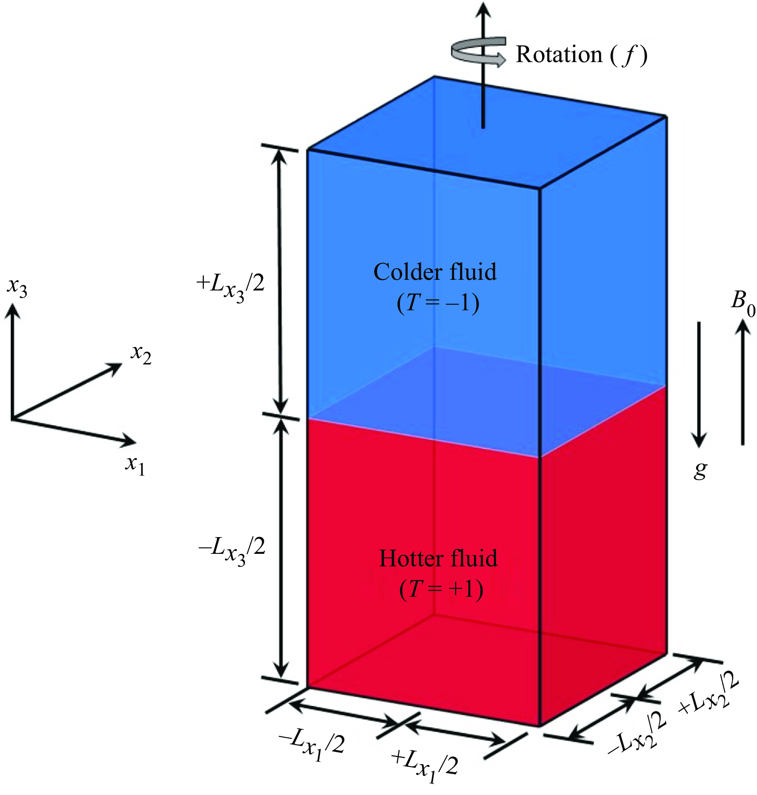
Sketch of the computational domain of RT configuration for electrically conducting miscible fluids, where the colder fluid of temperature
 $T=-1$
is placed above the hotter fluid of temperature
 $T=+1$
under gravity
 $g$
. This configuration is rotated about the vertical axis
 $x_3$
with uniform Coriolis’s frequency
 $f$
, and the uniform mean magnetic field
 $B_0$
is imposed normal to the interface between the colder and hotter fluid (or anti-parallel to
 $g$
).

2.1. Governing equations
We consider an unstable RT configuration of electrically conducting miscible fluids, where the colder fluid (temperature
 $T=-1$
) is supported by the hotter fluid (
 $T=1$
) against gravitational acceleration (
 $g$
) in a rectangular domain as shown in figure 1. This configuration is subject to rotation about the vertical axis (
 $x_3$
) with a constant Coriolis frequency
 $f$
. We impose a uniform mean magnetic field (
 $B_0$
), scaled as the Alfvèn velocity (Davidson Reference Davidson2013), normal to the initial interface and anti-parallel to
 $g$
. Here, we scale the magnetic field
 $\boldsymbol {B}$
 $(= (B_1, B_2, B_3))$
as a Alfvèn velocity
 $\boldsymbol {V}_{\!A}$
, such that
 $\boldsymbol {B}=\boldsymbol {V}_{\!A}= \boldsymbol {H}/\sqrt {\rho _0\mu _0}$
, where
 $\boldsymbol {H}$
is the true magnetic field,
 $\mu _0$
is the magnetic permeability and
 $\rho _0$
is the reference density (Davidson Reference Davidson2013). Under the Boussinesq and MHD approximations, the governing equations for an unsteady, incompressible, electrically conducting flow are given as (Biskamp Reference Biskamp2003; Naskar & Pal Reference Naskar and Pal2022a
,Reference Naskar and Pal
b
)
 \begin{equation} \frac {\partial u_j}{\partial x_j}=\frac {\partial B_j}{\partial x_j}=0, \end{equation}
 \begin{equation} \underbrace {\frac {\partial u_i}{\partial t}}_{\displaystyle \boldsymbol {F}_{\!I}} + \underbrace {u_j \frac {\partial u_i}{\partial x_j}}_{\displaystyle \boldsymbol {F}_{\!A}} = \underbrace {- \frac {\partial P}{\partial x_i}}_{\displaystyle \boldsymbol {F}_{\!P}} + \underbrace {f\epsilon _{ij3} u_j\hat {e}_3}_{\displaystyle \boldsymbol {F}_{\!C}} + \underbrace {B_j \frac {\partial B_i}{\partial x_j}}_{\displaystyle \boldsymbol {F}_{\!L}} + \underbrace {\beta g T\delta _{i3}}_{\displaystyle \boldsymbol {F}_{\!B}} + \underbrace {\nu \frac {\partial ^2 u_i}{\partial x_j \partial x_j}}_{\displaystyle \boldsymbol {F}_{\!V}}, \end{equation}
 \begin{equation} \frac {\partial {T}}{\partial t} + u_j \frac {\partial T}{\partial x_j}= \kappa \frac {\partial ^2 u_i}{\partial x_j \partial x_j}, \end{equation}
 \begin{equation} \frac {\partial {B_i}}{\partial t} + u_j \frac {\partial B_i}{\partial x_j}= B_j \frac {\partial u_i}{\partial x_j}+\mathcal {D}\frac {\partial ^2 B_i}{\partial x_j \partial x_j}. \end{equation}
Here,
 $\boldsymbol {u} = (u_1, u_2, u_3)$
is the velocity field vector,
 $P$
is the sum of the reduced pressure, magnetic pressure and centrifugal force, and the Cartesian coordinate system is denoted as
 $(x_1,x_2,x_3)$
. The different forces in the momentum equation (2.1b
) are identified as the inertial
 $\boldsymbol{F{\kern-2pt}}_I$
, the advection
 $\boldsymbol{F{\kern-2pt}}_A$
, the pressure gradient
 $\boldsymbol{F{\kern-2pt}}_P$
, the Coriolis
 $\boldsymbol{F{\kern-2pt}}_C$
, the Lorentz
 $\boldsymbol{F{\kern-2pt}}_L$
, the buoyancy
 $\boldsymbol{F{\kern-2pt}}_B$
and the viscous
 $\boldsymbol{F{\kern-2pt}}_V$
forces. The MHD approximation combines Maxwell’s equations of electrodynamics with Ohm’s law for a moving conductor, assuming that the charge density is vanishingly small for electrically conducting but non-magnetic fluids (see Davidson (Reference Davidson2013) for details). The Atwood number is considered small (
 $\mathcal {A}\simeq 0.102$
), representing small variations in density to ensure the validity of the Boussinesq approximation. In the case of Atwood numbers large enough to violate the Boussinesq approximation, the full compressible Navier–Stokes equations (Stone & Gardiner Reference Stone and Gardiner2007a
,Reference Stone and Gardiner
b
; Carlyle & Hillier Reference Carlyle and Hillier2017) are required to explore the dynamics of RT instability. In the limit of the Boussinesq approximation, the temperature field
 $T$
is related to density
 $\rho$
via the thermal expansion coefficient
 $\beta$
as
 $\rho =\rho _0 [1-\beta (T-T_0) ]$
, where
 $\rho _0$
and
 $T_0$
are the reference value of density and temperature, respectively. The fluid has kinematic viscosity
 $\nu$
, thermal diffusivity
 $\kappa$
and magnetic diffusivity
 $\mathcal {D}$
. Initially, at time
 $t=0$
, both the upper colder fluid (heavier of density
 $\rho _2$
) layer separated by the lower hotter fluid (lighter of density
 $\rho _1$
) layer are at rest, i.e.
 $T(\boldsymbol {x},0)=-({\theta _0}/{2}) sgn(x_3)$
and
 $\boldsymbol {u}(\boldsymbol {x},t)=0$
, where
 $\theta _0$
denotes the initial temperature jump across the layers that fix the Atwood number
 $\mathcal {A}= (\rho _2-\rho _1 )/ (\rho _2+\rho _1 )=\beta \theta _0/2$
(Boffetta & Mazzino Reference Boffetta and Mazzino2017). The mean magnetic field is imposed vertically (
 $B_0$
), such that
 $B_3(\boldsymbol {x},0)=B_0$
, while
 $B_1(\boldsymbol {x},0)=B_2(\boldsymbol {x},0)=0$
. Note that the vertical mean magnetic field (
 $B_0$
) is imposed at each time step. We seed initial perturbations by adding a
 $10\, \%$
of white noise to
 $T(\boldsymbol {x},0)$
in a small region around the interface at
 $x_3=0$
(centre of the vertical domain height).
We apply impenetrable and stress-free (free-slip) velocity boundary conditions at the top and bottom boundaries, written as
 \begin{equation} u_3=\frac {\partial u_1}{\partial x_3}=\frac {\partial u_2}{\partial x_3}=0 \quad \mathrm {at}\ x_3=\pm {L_{x_3}}/{2}, \end{equation}
where
 $L_{x_3}$
is the vertical domain height. We consider periodic boundary conditions in horizontal directions
 $x_1$
and
 $x_2$
for all the variables. The thermal boundary conditions are isothermal at the top and bottom boundaries, such that
 \begin{equation} T=1 \ \mathrm {(hot)}\quad \mathrm {at}\ x_3= -{L_{x_3}}/{2} \qquad \mathrm {and} \qquad T=-1 \ \mathrm {(cold)} \quad \mathrm {at}\ x_3= +{L_{x_3}}/{2}. \end{equation}
We use perfectly conducting boundary conditions for the magnetic field at the top and bottom boundaries as (Naskar & Pal Reference Naskar and Pal2022b )
 \begin{equation} \frac {\partial B_1}{\partial x_3}=\frac {\partial B_2}{\partial x_3}=0, \qquad B_3=B_0 \quad \mathrm {at}\ x_3=\pm {L_{x_3}}/{2}. \end{equation}
Since the horizontal directions are homogeneous, we perform Reynolds decomposition of all the variables
 $\mathcal {\phi }= \{u_i, P, T, B_i\}$
into a horizontally averaged mean component
 $\overline { \mathcal {\phi }}$
and fluctuating component
 $\mathcal {\phi }'$
, such that
 \begin{equation} \mathcal {\phi }({x_1,x_2,x_3},t)=\overline { \mathcal {\phi } }({x_3},t) + \mathcal {\phi }'({x_1,x_2,x_3},t), \end{equation}
 \begin{equation} \quad \overline {\mathcal {\phi }}({x_3},t)= \frac {1}{L_{x_1} L_{x_2}} \int _{-L_{x_2}/2}^{{+L_{x_2}/2}} \int _{-L_{x_1}/2}^{{+L_{x_1}/2}} \mathcal {\phi } ({x_1,x_2,x_3},t)\mathrm {d}x_1\mathrm {d}x_2. \end{equation}
Here, the overbar denotes the average in the horizontal directions, and
 $L_{x_1}$
and
 $L_{x_2}$
represent the domain lengths in
 $x_1$
and
 $x_2$
, respectively. We calculate root mean square (r.m.s.) of
 $\phi$
as
 \begin{equation} \phi _{r.m.s.}(x_3,t)=\left ( \overline {\phi '^2({x_1,x_2,x_3},t)}\right )^{1/2}, \end{equation}
where,
 $\phi '=\phi -\overline {\phi }$
from (2.5a
).
The spatial average of
 $\phi$
, denoted by the angled brackets (
 $\langle \phi \rangle$
), inside the mixing layer of height
 $h$
(defined later in § 3) is computed as
 \begin{equation} \langle \phi \rangle (t)= \frac {1}{h} \int _{-h/2}^{{+h/2}} \overline {\phi } ({x_3},t)\mathrm {d}x_3. \end{equation}
2.2. Numerical methodology and solver validation
The governing equations (2.1a
)–(2.1d
) are solved in a Cartesian coordinate system on a staggered grid arrangement, where the vector quantities (
 $\boldsymbol {u}$
and
 $\boldsymbol {B}$
) are stored at the cell faces, and scalar quantities (
 $T$
and
 $P$
) are stored at the cell centres, using the finite-difference method. All the spatial derivatives are computed using a second-order central finite-difference scheme, and the time advancement is performed using an explicit third-order Runge–Kutta method except for the diffusion terms, which are solved implicitly using the Crank–Nicolson method (Brucker & Sarkar Reference Brucker and Sarkar2010; Pal Reference Pal2020; Naskar & Pal Reference Naskar and Pal2022a
,Reference Naskar and Pal
b
; Singh & Pal Reference Singh and Pal2023). The projection method is employed to obtain the divergence-free velocity field where the pressure Poisson equation is solved using a parallel multigrid iterative solver to calculate the dynamic pressure. Similarly, to keep the magnetic field solenoidal, an elliptic divergence cleaning algorithm is employed (Brackbill & Barnes Reference Brackbill and Barnes1980). This numerical solver has been extensively validated and used for studies of turbulent mixing driven by Faraday instability (Singh & Pal Reference Singh and Pal2023, Reference Singh and Pal2024), three-phase flows (Singh et al. Reference Singh, Singh and Pal2023), rapidly rotating convection (RC)-driven dynamos (Naskar & Pal Reference Naskar and Pal2022a
,Reference Naskar and Pal
b
), RC (Pal & Chalamalla Reference Pal and Chalamalla2020) and several stratified free-shear and wall-bounded turbulent flows (Brucker & Sarkar Reference Brucker and Sarkar2010; Pal et al. Reference Pal, de, Matthew and Sarkar2013; Pal & Sarkar Reference Pal and Sarkar2015; Pal Reference Pal2020).
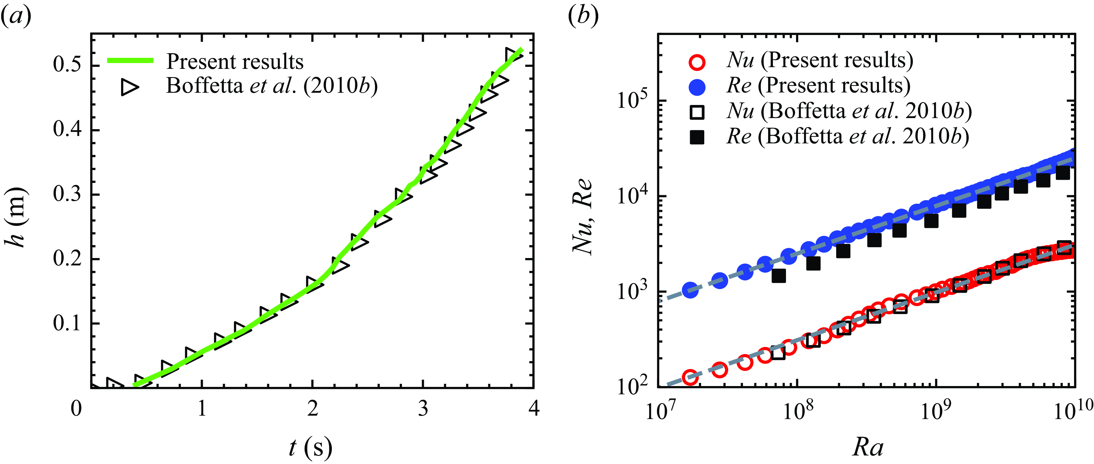
Comparison between present simulations and results obtained by Boffetta et al. (Reference Boffetta, Mazzino, Musacchio and Vozella2010b
) for (a) a temporal evolution of the mixing layer of height
 $h$
and (b) a spatially averaged Nusselt number (
 $Nu$
) and Reynolds number (
 $Re$
) as a function of the Rayleigh number (
 $Ra$
). These non-dimensional numbers are defined in (2.8). Dashed grey lines represent the ultimate state predictions, i.e.
 $Nu \simeq Ra^{1/2}Pr^{1/2}$
and
 $Re \simeq Ra^{1/2}Pr^{-1/2}$
scaling for
 $Pr=1$
(Boffetta et al. Reference Boffetta, Mazzino, Musacchio and Vozella2010b
).

We further validate our numerical solver by replicating the results of Boffetta et al. (Reference Boffetta, Mazzino, Musacchio and Vozella2010b
) for RT turbulence without rotation and a magnetic field. The simulation is performed in a horizontally periodic domain of size
 $L_{x_1}=L_{x_2}$
and
 $L_{x_3}=4L_{x_1}$
with uniform grids
 $N_{x_1}=N_{x_2}=512$
and
 $N_{x_3}=2048$
. Other parameters are
 $\beta g=2.0$
,
 $\theta _0=1$
,
 $\nu =\kappa =4.8 \times 10^{-6}$
. The comparison between the results obtained in the present simulations and the results of Boffetta et al. (Reference Boffetta, Mazzino, Musacchio and Vozella2010b
) for the temporal evolution of the mixing layer height (
 $h$
) is shown in figure 2(a) and for the Nusselt number (
 $Nu$
) and Reynolds number (
 $Re$
) as a function of Rayleigh number (
 $Ra$
) is shown in figure 2(b). These non-dimensional numbers are defined as
 \begin{equation} Nu=1+\frac {\langle u_3^{\prime } T' \rangle h}{\kappa \theta _0}, \qquad\!\!\! Re=\frac {\sqrt {(u_{1,r.m.s.}^2+u_{2,r.m.s.}^2+u_{3,r.m.s.}^2)}\ h}{\nu } \quad \mathrm {and} \quad Ra=\frac {\beta g \theta _0 h^3}{\nu \kappa }. \end{equation}
Here,
 $u_3^{\prime }$
is the fluctuating vertical velocity,
 $T'$
is fluctuating temperature,
 $\langle \ \rangle$
is the spatial average inside
 $h$
(defined in (2.7)), the r.m.s. (defined in (2.6)) horizontal
 $u_{1,r.m.s.}$
,
 $u_{2,r.m.s.}$
and vertical
 $u_{3,r.m.s.}$
velocities are taken at the mid-plane
 $x_3=0$
. The mixing layer height
 $h$
is measured based on the threshold on the horizontally averaged mean temperature profile, such that
 $\bar {T} (\pm h/2) = \mp 0.8 \theta _0/2$
. We can observe that our results match the results of Boffetta et al. (Reference Boffetta, Mazzino, Musacchio and Vozella2010b
).
We also show the validation of our solver by reproducing the results of non-magnetic RC and rotating dynamo convection (DC) of Stellmach & Hansen (Reference Stellmach and Hansen2004) in a rotating plane layer of an electrically conducting fluid confined between two parallel plates, heated from the bottom and cooled from the top (see Naskar & Pal Reference Naskar and Pal2022a for details) in the Appendix.
2.3. Problem set-up and simulation parameters
We perform all simulations in the computational domain of size
 $L_{x_1}=L_{x_2}=2\pi \:\textrm{m}$
in the horizontal directions and
 $L_{x_3}=4.32\pi \:\textrm{m}$
, which includes a sponge region of thickness
 $L_s\simeq 0.2\pi \:\textrm{m}$
utilising
 $20$
grid points at the top and bottom boundaries (
 $x_3$
). These sponge regions are employed near the top and bottom boundaries to control the spurious reflections from the disturbances propagating out of the domain, where damping functions gradually relax the values of the velocities to their corresponding values at the boundary (Singh & Pal Reference Singh and Pal2023). This is accomplished by adding the damping functions to the right-hand side of the momentum equation (2.1b
), as explained in Brucker & Sarkar (Reference Brucker and Sarkar2010). The sponge region is always kept sufficiently far away from the mixing zone and, therefore, does not affect the dynamics of the mixing of fluids. We use uniform grids
 $N_{x_1}=N_{x_2}=1024$
in the horizontal direction, while non-uniform grids
 $N_{x_3}=1536$
are used in the vertical direction
 $x_3$
. The grids are clustered at the vertical centre region of thickness
 $\simeq 2.23\pi \:\mathrm {m}$
with
 $\Delta x_{3_{min}}=\Delta x_1=\Delta x_2$
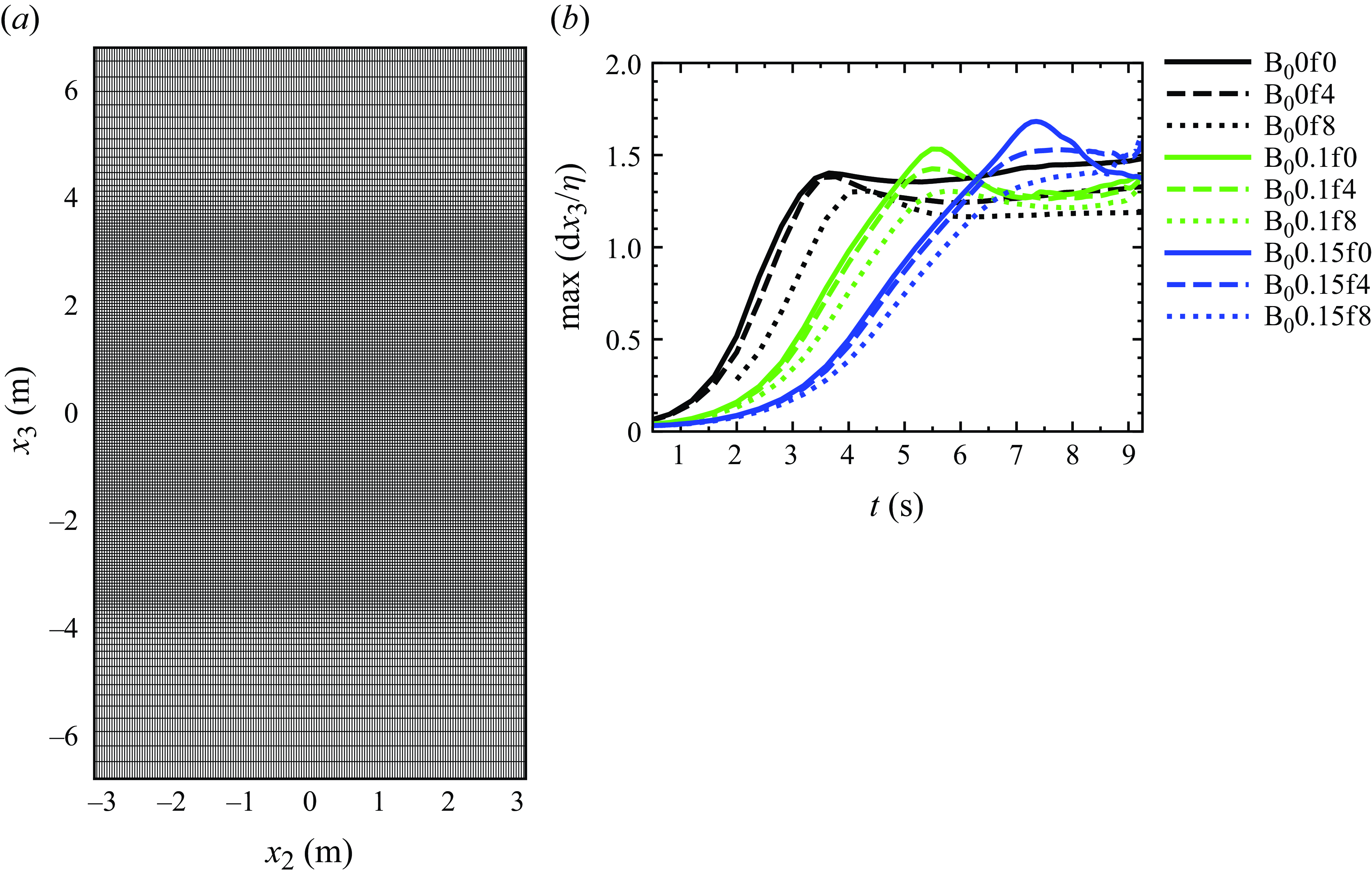
as illustrated in figure 3(a). This grid arrangement maintains a
 $\max({\rm d}x_3/\eta ) \lt 2$
(Brucker & Sarkar Reference Brucker and Sarkar2010), where
 $\eta$
is the Kolmogorov scale
 $ (\eta = (\nu ^3/\epsilon _v )^{1/4} )$
, as shown in figure 3(b), which is fine enough to resolve all the length scales in the mixing region. Here
 $\nu$
is the kinematic viscosity and
 $\epsilon _v$
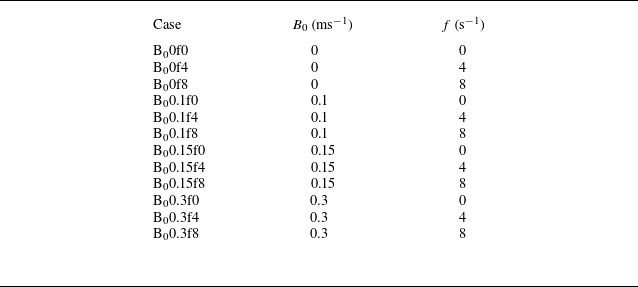
is the horizontally averaged viscous dissipation rate, which is defined later in (3.8). We summarise all the parameters for different simulation cases in table 1. Hereafter, we refer to non-magnetic (
 $B_0 = 0$
) cases as HD cases and magnetic (
 $B_0 \neq 0$
) cases as MHD cases. We refer to each simulation case with a unique name; for example, the B
 $_0$
0.1f4 case represents
 $B_0=0.1\,\mathrm {ms^{-1}}$
and
 $f=4\,\mathrm {s^{-1}}$
.
(a) Grid clustering at the vertical centre region for resolving all the length scales in the mixing layer shown in the vertical
 $x_2-x_3$
centre plane (
 $x_1=0$
). (b) Temporal evolution of the maximum vertical grid spacing
 ${\rm d}x_3$
normalised with the Kolmogorov length scale
 $\eta =(\nu ^3/\epsilon _v)^{1/4}$
for non-rotation and rotation cases with
 $B_0=0,0.1,0.15\,\mathrm {ms^{-1}}$
. Here
 $\nu$
is the kinematic viscosity and
 $\epsilon _v$
is the horizontally averaged viscous dissipation rate (defined later in (3.8)).

Simulation parameters: for all cases, we use
 $\mathcal {A}g=\beta \theta _0 g/2=1.0\:\mathrm {m\:s^{-2}}$
,
 $g=9.81\:\mathrm {m\:s^{-2}}$
,
 $\theta _0=2$
, kinematic viscosity
 $\nu$
, thermal diffusivity
 $\kappa$
and magnetic diffusivity
 $\mathcal {D}$
respectively are
 $\nu =\kappa =\mathcal {D}=3\times 10^{-4}\:\mathrm {m^2\:s^{-1}}$
, such that the Prandtl number
 $Pr=\nu / \kappa =1$
and the magnetic Prandtl number
 $Pr_m=\nu /\mathcal {D}=1$
.

Instantaneous temperature contours in the vertical
 $x_2{-}x_3$
centre plane (
 $x_1=0$
) for (a) the non-rotating HD case B
 $_0$
0f0 (first leftmost column), (b) the rotating HD case B
 $_0$
0f8 (second column), (c) the non-rotating MHD case B
 $_0$
0.15f0 (third column), and (d) the rotating MHD case B
 $_0$
0.15f8 (fourth column) at different time instants. The blue colour represents cold fluid (
 $T=-1$
), and the red colour represents hot fluid (
 $T=1$
).

3. Results
3.1. Flow structures
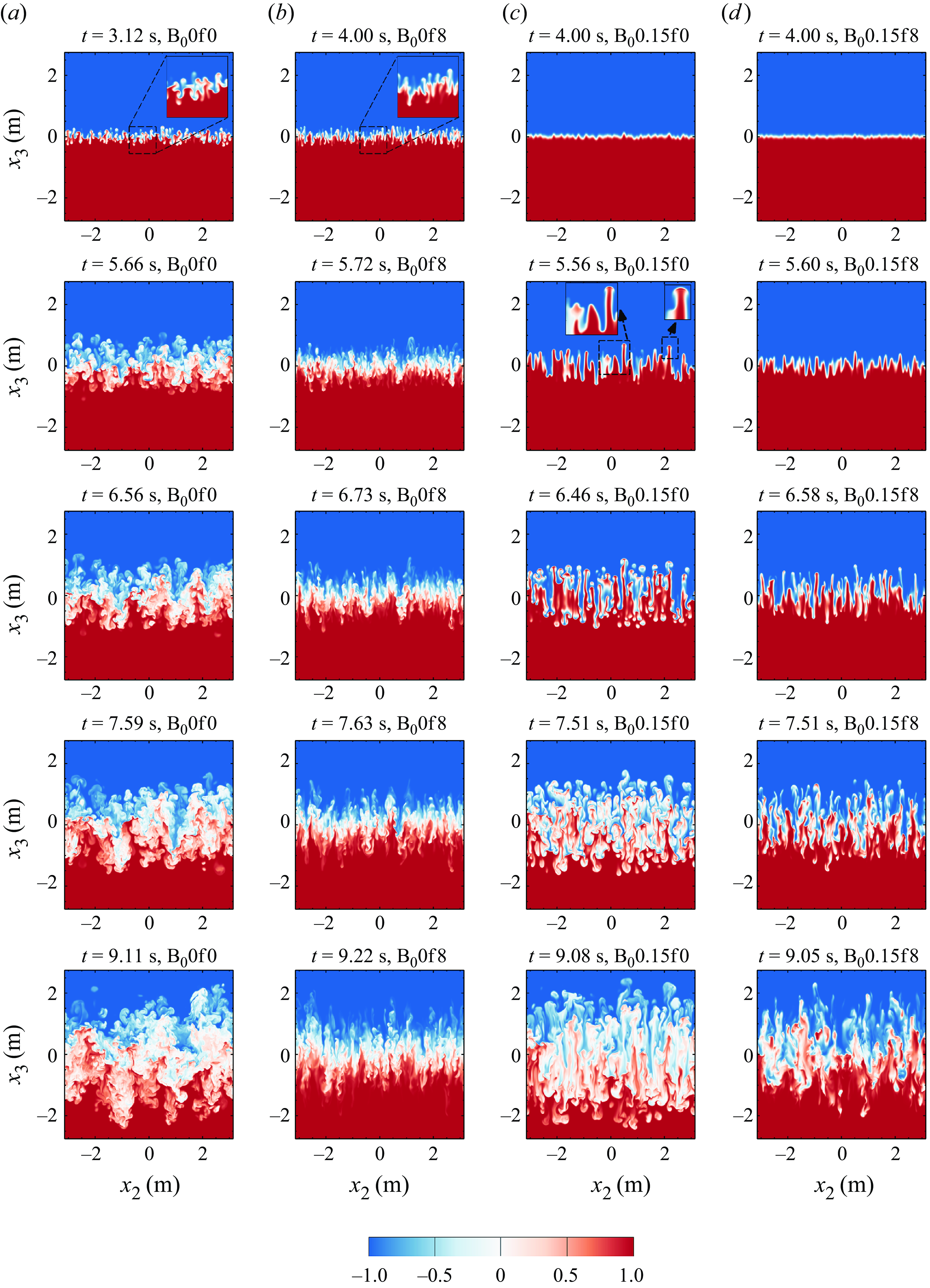
To qualitatively illustrate the effect of the imposed vertical mean magnetic field and rotation on the formation and evolution of flow structures, we show snapshots of the temperature field (
 $T$
) at different time instants for the non-rotating HD B
 $_0$
0f0, rotating HD B
 $_0$
0f8, non-rotating MHD B
 $_0$
0.15f0 and rotating MHD B
 $_0$
0.15f8 cases in figures 4(a), 4(b), 4(c) and 4(d), respectively. For the non-rotating HD case B
 $_0$
0f0, the initial perturbed interface becomes unstable to the downward acting gravitational accelerations (
 $g$
) (or RT instability), resulting in the growth of perturbations. This leads to the emergence of small-scale rising (hot fluid) and sinking (cold fluid) thermal plumes with mushroom-shaped caps at their tips, as depicted in the enlarged view in figure 4(a) at
 $t=3.12$
s. These caps are attributed to the secondary KH instability generated by the relative motion between the plumes (Sharp Reference Sharp1984; Jun et al. Reference Jun and Norman1995; Abarzhi Reference Abarzhi2010; Zhou Reference Zhou201
Reference Zhou7
Reference Zhou
a
,Reference Zhou
b
). The plumes start interacting nonlinearly with each other, penetrating the opposite region (see figure 4(a) at
 $t=5.66$
s) and hence, enhancing the heat transfer between the fluids. Eventually, mixing occurs, the flow becomes turbulent and the mixing layer grows continuously due to the conversion of potential energy into turbulent kinetic energy (Cabot & Cook Reference Cabot and Cook2006; Boffetta & Mazzino Reference Boffetta and Mazzino2017; Boffetta & Musacchio Reference Boffetta and Musacchio2022). The evolution of the turbulent mixing layer is illustrated at
 $t=6.56$
s,
 $7.59$
s and
 $9.11$
s in figure 4(a). At a high rotation rate
 $f=8\,\mathrm {s^{-1}}$
(HD case B
 $_0$
0f8), the formation of mushroom-shaped caps at the plume tips is inhibited, reducing the deformation of the plumes and their horizontal interactions with each other, as depicted by the enlarged view in figure 4(b) at
 $t=4$
s. This signifies that the Coriolis force stabilises the flow, and forms coherent and vertically elongated thermal plumes as apparent at all time instants in figure 4(b). These elongated thermal plumes indicate the presence of the Taylor–Proudman constraint imposed by the Coriolis force (as explored later through force analysis), which prevents changes along the rotational axis, resulting in a 2-D flow. Additionally, the Coriolis force reduces the mixing layer thickness owing to the damping of fluctuations in the vertical velocity compared to the non-rotating case B
 $_0$
0f0, suggesting a reduction in heat transfer. This can be observed by comparing figure 4(a) for the B
 $_0$
0f0 case with figure 4(b) for the B
 $_0$
0f8 case at the same time instants. Supplementary movies 1 and 2, available at https://doi.org/10.1017/jfm.2025.191, demonstrate the flow evolution for B
 $_0$
0f0 and B
 $_0$
0f8, respectively. Boffetta et al. (Reference Boffetta, Mazzino and Musacchio2016) and Wei et al. (Reference Wei, Li, Wang, Yang, Zhu, Qian and Luo2022) also report similar effects of rotation.
The inclusion of a mean vertical magnetic field
 $B_0=0.15\,\mathrm {ms^{-1}}$
significantly modifies the formation and growth of the thermal plumes in both the non-rotating (
 $f=0$
) and rotating (
 $f=8\,\mathrm {s^{-1}}$
) cases, as demonstrated in figures 4(c) and 4(d), respectively. For the non-rotating MHD case B
 $_0$
0.15f0, in the initial (linear) phase, perturbations are vertically stretched by the mean magnetic field, as depicted in figure 4(c) at
 $t=4$
s, followed by the emergence of plumes. In contrast to B
 $_0$
0.15f0, the plumes in cases B
 $_0$
0f0 and B
 $_0$
0f8 have already been formed and achieved a significant growth till
 $t=4$
s, signifying the imposed magnetic field delays the onset of the instability. We define the onset of the RT instability as the time instant when the mixing layer begins to grow. Since the imposed magnetic field acts tangentially to the sheared interface of the vertically stretched perturbations, the secondary shear instabilities at small scales are inhibited (as discussed later), preventing the interactions between the perturbations. Consequently, the vertically stretched perturbations transform to smooth vertically elongated plumes, followed by their rapid growth, as reported by Jun et al. (Reference Jun, Norman and Stone1995) using linear theory and 2-D simulations and Briard et al. (Reference Briard, Gréa and Nguyen2022, Reference Briard, Gréa and Nguyen2024) using 3-D simulations. Later, the shear instabilities are triggered, which destabilises the smooth elongated plumes, leading to the emergence of mushroom-shaped caps at their tips, as indicated in the enlarged views at
 $t\simeq 5.56$
s in figure 4(c), similar to that reported by Briard et al. (Reference Briard, Gréa and Nguyen2022, Reference Briard, Gréa and Nguyen2024). The elongated plumes signify collimation of flow along the magnetic field lines in the vertical direction and indicate that the imposed magnetic field reduces the interactions between the thermal plumes. With time evolution, the rapid vertical stretching of the plumes continues, and the relative velocity becomes significant enough to enhance the strength of shear instabilities, resulting in the clear formation of mushroom-shaped caps, as shown at
 $t=6.46$
s in figure 4(c). Eventually, these caps begin to detach from their respective plumes due to vertical stretching followed by the full breakup of the sheared thin plumes into small structures as observed in figure 4(c) at
 $t=7.51$
s (see supplementary movie 3). Consequently, the flow becomes turbulent, which remains weaker than in the HD case B
 $_0$
0f0 because the fluid structures are still collimated along the magnetic field lines in the vertical direction, as apparent at
 $t\simeq 9.08$
s in figure 4(c). However, this flow collimation in the B
 $_0$
0.15f0 case results in the increased height of the mixing layer, enhancing the heat transfer as compared to the HD cases.
When rotation
 $f=8\,\mathrm {s^{-1}}$
is added along with
 $B_0=0.15\,\mathrm {ms^{-1}}$
(MHD case B
 $_0$
0.15f8), the Coriolis force also plays a significant role by adding its stabilisation effect that damps the growth of the elongated plumes, as can be observed by comparing figures 4(d) and 4(c) for the B
 $_0$
0.15f8 and B
 $_0$
0.15f0 cases, respectively, at
 $t=4.0$
s and
 $5.6$
s. Additionally, the rotation inhibits the formation of mushroom-shaped caps that were observed in the non-rotating case B
 $_0$
0.15f0 (see a comparison among figures 4(d) and 4(c) at
 $t\simeq 6.5$
s). The continued vertical stretching owing to the imposed magnetic field results in the thinning of plumes, eventually causing them to break down as illustrated in figure 4(d) at
 $t=7.51$
s,
 $9.05$
s (see supplementary movie 4). The comparison between figures 4(c) at
 $t=9.08$
s and 4(d) at
 $t=9.05$
s indicates that the mixing and turbulence in the flow is weaker in the B
 $_0$
0.15f8 case than that in the B
 $_0$
0.15f0 case, signifying the damping of velocity fluctuations and heat transfer by the Coriolis force.
These qualitative results show the strong impact of the combined vertically imposed mean magnetic field and rotation on the flow structures’ development and evolution, which can influence the heat transport between the hot and cold fluids. Next, we quantitatively analyse the temporal growth of the mixing layer (§ 3.2) to understand and quantify the heat transport (§ 3.5).
3.2. Temporal evolution of the mixing layer
Temporal evolution of the mixing layer height
 $h$
for non-rotating and rotating (a) HD cases, (b) HD and MHD at
 $B_0=0.1\,\mathrm {ms^{-1}}$
cases, (c) HD and MHD at
 $B_0=0.15\,\mathrm {ms^{-1}}$
cases, and (d) HD and MHD at
 $B_0=0.3\,\mathrm {ms^{-1}}$
cases. Insets in (a) and (b) correspond to the onset of RT instability.

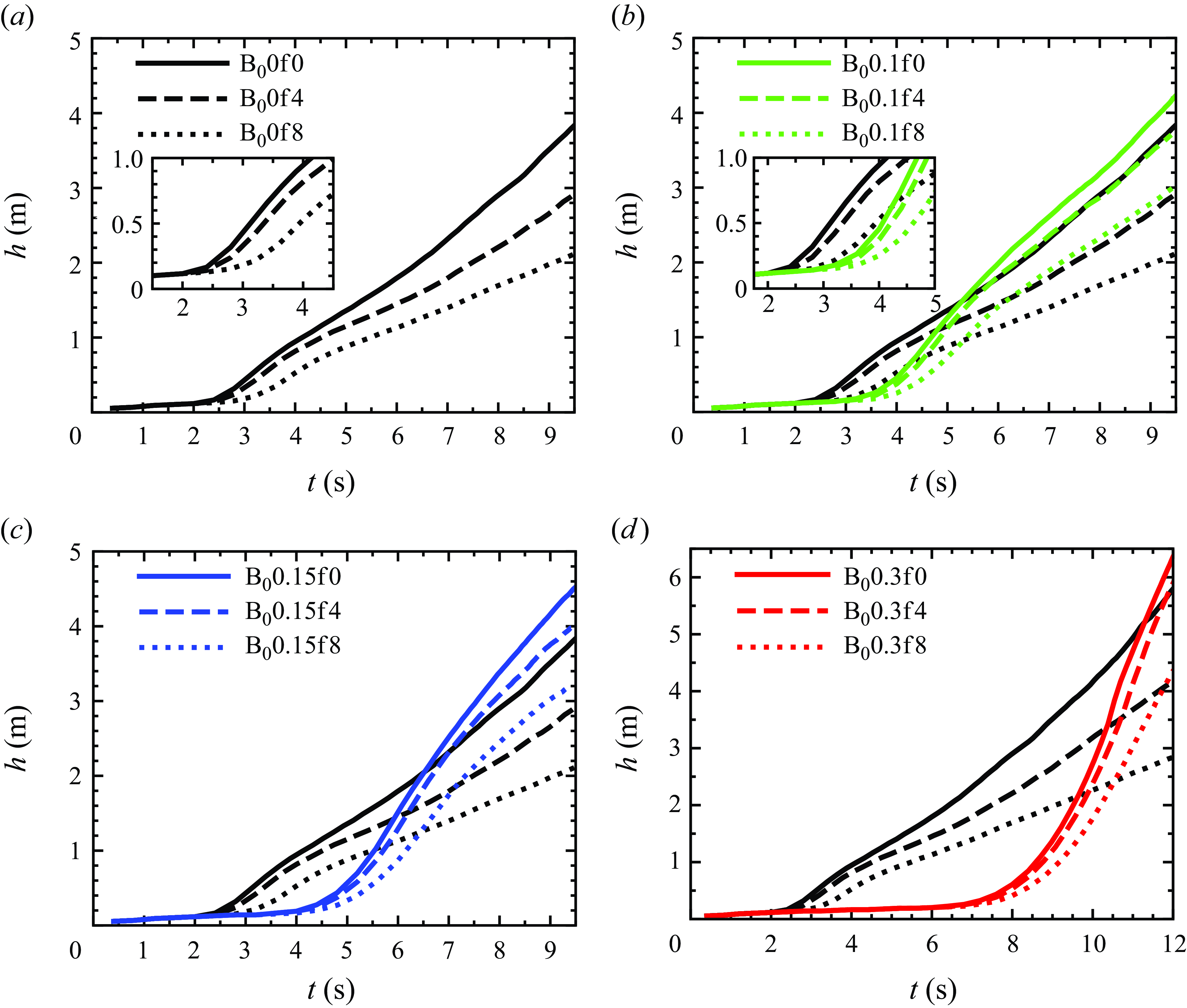
In this subsection, to quantitatively assess the flow evolution under the influence of the magnetic field and rotation, we evaluate the height of the mixing layer (
 $h$
) as a function of time in figure 5. The mixing layer height is calculated based on the threshold value of
 $x_3$
at which
 $\overline { T}(x_3,t)$
reaches a fraction
 $r$
of the maximum value, such that
 $\overline { T}(\pm x_3,t)=\mp r \theta _0$
, where
 $r=0.9$
(Boffetta et al. Reference Boffetta, Mazzino and Musacchio2016). We show the temporal evolution of
 $h$
for the non-rotating and rotating HD cases in figure 5a, and compare this evolution between the HD and MHD cases for
 $B_0=0.1$
,
 $0.15$
and
 $0.3\,\mathrm {ms^{-1}}$
in figures 5(b), 5(c) and 5(d), respectively. For the non-rotating HD case B
 $_0$
0f0,
 $h$
starts to grow at
 $t\simeq 2.5$
s with the emergence of thermal plumes, followed by the rapid growth in the turbulent regime (see figure 5
a). With the addition of a rotation rate of
 $f=4\,\mathrm {s^{-1}}$
(HD case B
 $_0$
0f4), the growth rate of
 $h$
is damped compared to the B
 $_0$
0f0 case. This damping becomes stronger as
 $f$
increases from
 $4$
to
 $8\,\mathrm {s^{-1}}$
(B
 $_0$
0f8 case) due to the increased stabilisation effect exerted by the Coriolis force. Additionally,
 $h$
starts increasing at
 $t\simeq 3{-}3.5$
s (see inset of figure 5
a) for the B
 $_0$
0f8 case, whereas for B
 $_0$
0f0 and B
 $_0$
0f4 the growth starts at
 $t\simeq 2.5$
s, signifying that the Coriolis force delays the onset of the instability at high rotation rates.
When the vertical mean magnetic field
 $B_0=0.1\,\mathrm {ms^{-1}}$
is imposed in the absence of rotation (
 $\textrm{B}_0$
0.1f0 case),
 $h$
starts growing at
 $t\simeq 3.5{-}4$
s signifying the delay in the onset of instability compared to the HD B
 $_0$
0f0 case where
 $h$
starts growing at
 $t\simeq 2.5$
s (see figure 5
b). We can observe a rapid increase in
 $h$
for B
 $_0$
0.1f0, which eventually exceeds the
 $h$
for B
 $_0$
0f0. This initial rapid growth of
 $h$
is due to the formation of vertically elongated plumes by
 $B_0$
, which tend to inhibit plume interactions, allowing them to grow rapidly. Eventually, these plumes break into smaller structures and the flow enters the turbulent regime where it remains collimated along the vertical magnetic field lines, leading to the observed enhancement in
 $h$
for the B
 $_0$
0.1f0 case compared to the B
 $_0$
0f0 case. Similar observations were reported by Briard et al. (Reference Briard, Gréa and Nguyen2024) for their non-rotating MHD simulations.
Inclusion of rotation,
 $f=4\,\mathrm {s^{-1}}$
, with
 $B_0=0.1\,\mathrm {ms^{-1}}$
(B
 $_0$
0.1f4 case) reduces the growth of
 $h$
compared to the non-rotating case B
 $_0$
0.1f0. This reduction becomes more pronounced when
 $f=8\,\mathrm {s^{-1}}$
(figure 5
b) due to the damping of the growth of vertically elongated plumes in the initial regime and the small-scale flow structures in the turbulent regime by the strong stabilisation effect of the Coriolis force. Owing to the flow collimation along the vertical magnetic field lines in MHD cases,
 $h$
for B
 $_0$
0.1f4 and B
 $_0$
0.1f8 remain higher than the corresponding HD B
 $_0$
0f4 and B
 $_0$
0f8 cases, respectively. For
 $f=0$
, with
 $B_0=0.15\,\mathrm {ms^{-1}}$
(figure 5
c) and
 $B_0=0.3\,\mathrm {ms^{-1}}$
(figure 5
d),
 $h$
begins to grow at
 $t\simeq 4{-}4.5$
s and
 $t\simeq 7{-}7.5$
s, respectively, revealing that the delay in the onset of instability increases with an increase in the strength of the imposed magnetic field, which is consistent with the predictions of linear theory in the sense that the growth of instability reduces as
 $B_0$
increases in the linear phase (Chandrasekhar Reference Chandrasekhar1968; Jun et al. Reference Jun, Norman and Stone1995). However, at later times, after experiencing rapid growth,
 $h$
becomes larger with an increase in
 $B_0$
from
 $0.15$
to
 $0.3\,\mathrm {ms^{-1}}$
(B
 $_0$
0.15f0 and B
 $_0$
0.3f0), compared to the cases with
 $B_0=0,\ 0.1\,\mathrm {ms^{-1}}$
for
 $f=0$
(see the comparison among figures 5
b, 5
c and 5
d). This enhancement is attributed to the increased tendency of
 $B_0$
(
 $=0.15,\,0.3\,\mathrm {ms^{-1}}$
) to collimate the flow along the vertical magnetic field lines, resulting in stronger vertical stretching of the plumes. Similar to the rotating MHD cases B
 $_0$
0.1f4 and B
 $_0$
0.1f8, the growth of
 $h$
decreases for B
 $_0$
0.15f4 and B
 $_0$
0.15f8 (B
 $_0$
0.3f4 and B
 $_0$
0.3f8) cases compared to the corresponding non-rotating MHD B
 $_0$
0.15f0 (B
 $_0$
0.3f0) cases, due to the stabilisation effect of the Coriolis force. Since the vertical elongation of the plumes is stronger at
 $B_0=0.15\,\mathrm {ms^{-1}}$
than at
 $B_0=0.1\,\mathrm {ms^{-1}}$
,
 $h$
is higher in the B
 $_0$
0.15f4 and B
 $_0$
0.15f8 cases compared to the B
 $_0$
0.1f4 and B
 $_0$
0.1f8 cases, respectively (see the comparison between figures 5
b and 5
c). Additionally, during the initial growth,
 $h$
grows more rapidly with the increasing strength of
 $B_0$
in both the non-rotating and rotating cases.
In the nonlinear state, the self-similar regime of the RT instability in the absence of both the rotation and magnetic field is characterised by the quadratic time evolution of the mixing layer height
 $h$
, i.e.
 $h = 2\alpha \mathcal {A}gt^2$
(Youngs Reference Youngs1994; Ristorcelli & Clark Reference Ristorcelli and Clark2004), where
 $\alpha$
is the growth rate. In the turbulent regime, the quadratic growth of
 $h$
is recovered for both the non-rotating HD and MHD cases with
 $B_0=0.1,0.15\,\mathrm {ms^{-1}}$
, similar to that reported by Briard et al. (Reference Briard, Gréa and Nguyen2024). However, the rotating HD cases show the deviation from the quadratic growth of
 $h$
due to the damping of the growth of the mixing layer by the Coriolis force, consistent with the observations of Wei et al. (Reference Wei, Li, Wang, Yang, Zhu, Qian and Luo2022) who obtained two different scaling laws between the
 $h$
and dimensionless time at various strengths of dimensionless rotation. We observe a small deviation from the quadratic growth of
 $h$
at the end of simulations in rotating MHD cases with
 $B_0=0.1,0.15\,\mathrm {ms^{-1}}$
. This indicates that similar to the observations of Wei et al. (Reference Wei, Li, Wang, Yang, Zhu, Qian and Luo2022) for rotating HD cases, the RT instability in rotating MHD cases may also exhibit different scaling laws that can be confirmed at stronger rotation rates of
 $f\gt 8\,\mathrm {s^{-1}}$
and may be of interest for future studies.
Vertical variation of the squared r.m.s
. vertical velocity
 $u_{3,r.m.s.}$
normalised by the squared mean vertical magnetic field
 $B_0$
, scaled as the Alfvèn velocity, for the non-rotating MHD cases (a) B
 $_0$
0.15f0 and (b) B
 $_0$
0.3f0 at different time instants.

3.3. Secondary shear instability
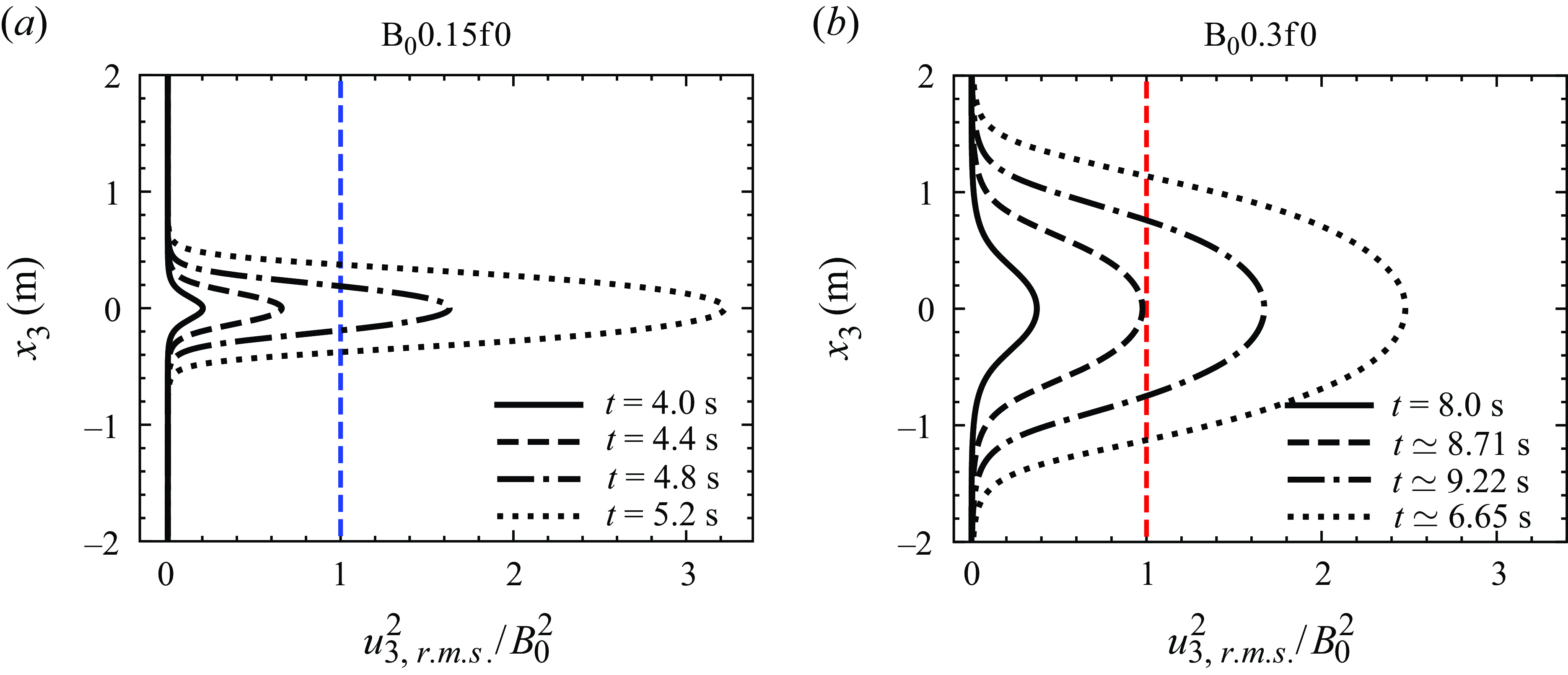
As observed qualitatively in § 3.1, we investigate the inhibition of secondary small-scale shear instabilities in the initial phase of RT instability owing to the vertically imposed magnetic field in the present subsection. We plot the vertical profiles of the squared r.m.s. vertical velocity (
 $u_{3,r.m.s.}^2$
) normalised by the
 $B_0^2$
(scaled as the Alfvèn velocity), for the non-rotating MHD cases B
 $_0$
0.15f0 and B
 $_0$
0.3f0 in figures 6(a) and 6(b), respectively, at different time instants. Jun et al. (Reference Jun and Norman1995) proposed that for the vertically imposed mean magnetic field case, if the square of the relative velocity of the plumes is smaller than the squared Alfvèn velocity, then the secondary shear instabilities (KH instabilities) are suppressed, and there is no flow transverse to the gravity vector. Briard et al. (Reference Briard, Gréa and Nguyen2024) also provided a similar criterion by performing a simplified linear stability analysis within a 2-D inviscid framework and comparing it with their DNS. For B
 $_0$
0.15f0, figure 6(a) illustrates that
 $u_{3,r.m.s.}^2/B_0^2 \lt 1$
Until
 $t=4.4$
s, suggesting that although the perturbations at the interface stretch to take the shape of elongated plumes, shear instabilities are not triggered. At
 $t = 4.8$
s and beyond, the plumes are destabilised by the onset of shear instabilities as also indicated in the enlarged views in figure 4(c) at
 $t=5.56$
s (see supplementary movie 3). For B
 $_0$
0.3f0,
 $u_{3,r.m.s.}^2/B_0^2 \lt 1$
until
 $t=8.71$
s and is
 ${\gt } 1$
beyond it. In this case, the instability is already triggered by
 $t=8.71$
s, and the height of the mixing layer is
 $h\simeq 1.2$
m at
 $t=8.71$
s (figure 5
d). In contrast to the B
 $_0$
0.15f0 case,
 $h$
is approximately three times larger for the B
 $_0$
0.3f0 case until
 $u_{3,r.m.s.}^2/B_0^2 \lt 1$
. This signifies that for B
 $_0$
0.3f0, the plumes have already reached greater heights than B
 $_0$
0.15f0 before triggering shear instabilities. Consequently, large, smooth, vertically elongated plumes form in B
 $_0$
0.3f0 (see supplementary movie 5).


3.4. Quantification of mixing and growth rates of the mixing layer height
In this subsection we first quantify the degree to which the hot and cold fluids are mixed using the mixing parameter
 $\Theta$
(Youngs Reference Youngs1994; Zhou Reference Zhou2024) given by
 \begin{equation} \Theta = \frac {\displaystyle \int \overline {\left (\theta _0/2-T\right )\left (\theta _0/2+T\right )} {\rm d}x_3}{\displaystyle \int \overline {\left (\theta _0/2-T\right )} \, \, \overline {\left (\theta _0/2+T\right )} {\rm d}x_3} = 1-\frac {\displaystyle \int \overline {{T^{\prime }}^2}{\rm d}x_3}{\displaystyle \int {\left (\theta _0/2-\overline {T}\right ) \left (\theta _0/2+\overline {T}\right )} {\rm d}x_3}. \end{equation}
Here,
 $\Theta$
can vary between 0 and 1, with
 $\Theta =0$
corresponding to unmixed fluids and
 $\Theta =1$
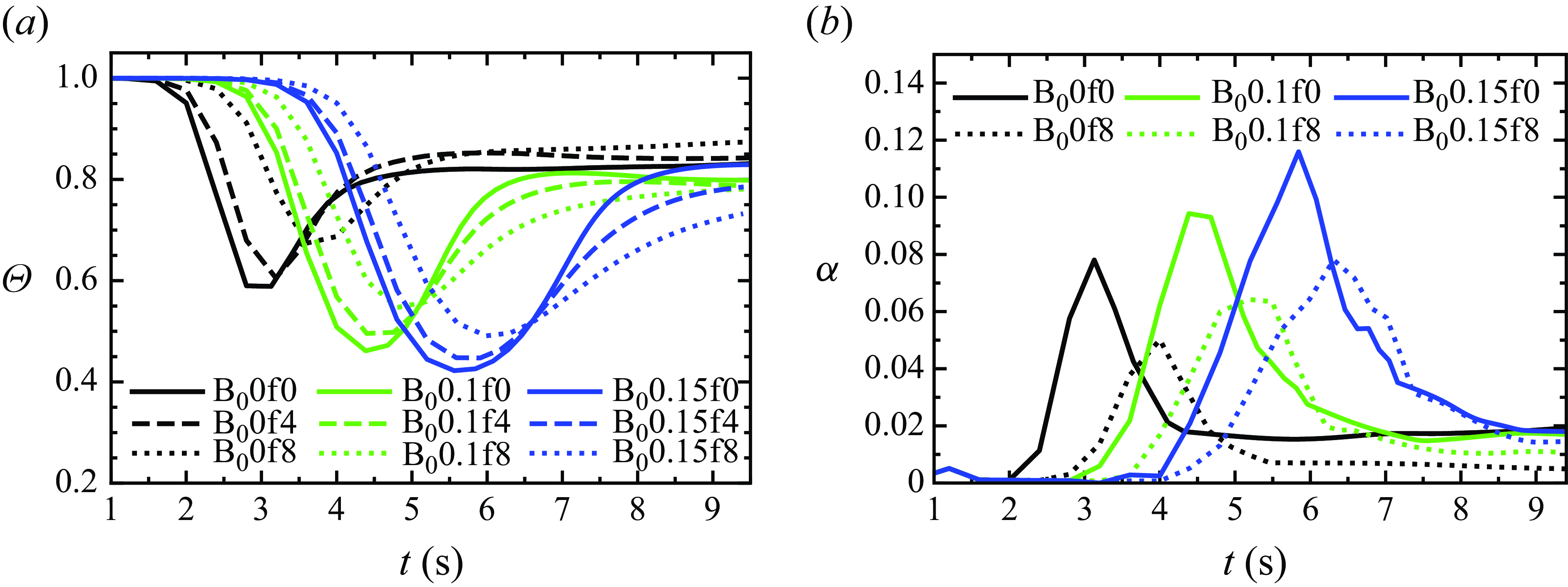
corresponding to completely mixed fluids. Figure 7(a) shows the temporal variation of
 $\Theta$
for the non-rotating and rotating HD and MHD (
 $B_0=0.1, 0.15\,\mathrm {ms^{-1}}$
) cases. At the beginning of each case, the mixing layer grows due to laminar diffusion and
 $\Theta \simeq 1$
reflects the complete mixing of the fluids within the layer during this diffusive growth phase (Cook & Dimotakis Reference Cook and Dimotakis2001). As the hot and cold fluids interpenetrate, stirring occurs without mixing, and
 $\Theta$
decreases. After reaching a minimum value,
 $\Theta$
increases again, indicating an increase in mixing and a transition to turbulence, eventually reaching an asymptotic state. In the non-rotating HD case (B
 $_0$
0f0), the final value of
 $\Theta$
is
 $\simeq 0.83$
, which agrees well with previous studies (Ramaprabhu et al. Reference Ramaprabhu, Dimonte and Andrews2005; Ristorcelli & Clark Reference Ristorcelli and Clark2004; Briard et al. Reference Briard, Gréa and Nguyen2024). In the rotating HD cases, the final value of
 $\Theta$
increases to
 $\simeq 0.842$
and
 $0.875$
with increasing rotation strengths to
 $f=4$
and
 $8\,\mathrm {s^{-1}}$
, respectively, similar to the findings of Wei et al. (Reference Wei, Li, Wang, Yang, Zhu, Qian and Luo2022). This suggests that rotation results in enhanced mixing. The reason for this enhancement is rotation’s inhibition of the formation of mushroom-shaped caps at the plume tips during the initial growth phase (see figure 4(b) at
 $t=4$
s). Without this inhibition, the caps would engulf large parcels of pure fluid, hindering mixing, as observed in the non-rotating case B
 $_0$
0f0 (Cabot & Cook Reference Cabot and Cook2006). This reasoning is supported by the observation that the minimum value of
 $\Theta$
, corresponding to transition to turbulence, is higher in the B
 $_0$
0f8 case (
 $\Theta \simeq 0.68$
at
 $t \simeq 3.7$
s) than in the B
 $_0$
0f0 case (
 $\Theta \simeq 0.59$
at
 $t \simeq 3$
s). This enhancement in mixing (
 $\Theta$
) is further reflected in the asymptotic state, facilitated by the coherent, vertically elongated structures (see figure 4
b).
In the non-rotating MHD case with weaker
 $B_0 = 0.1\, \mathrm {ms^{-1}}$
, the final value of
 $\Theta$
 $(\simeq 0.8)$
is smaller than that in the corresponding HD case B
 $_0$
0f0 (
 $\Theta \simeq 0.83$
). This indicates the reduction in mixing due to the effect of
 $B_0$
, which collimates flow structures along vertical magnetic lines, limiting their interactions. Since rotation inhibits the formation of mushroom-shaped caps at the plume tips, we observe an enhancement in mixing at the time of transition to turbulence in the rotating MHD case B
 $_0$
0.1f8 relative to the non-rotating case B
 $_0$
0.1f0. This is evident from figure 7(a), where the minimum value of
 $\Theta$
(
 $\simeq 0.55$
at
 $t \simeq 4.8$
s) in B
 $_0$
0.1f8 is greater than the non-rotating case B
 $_0$
0.1f0 (
 $\Theta \simeq 0.47$
at
 $t \simeq 4.5$
s). However, this enhancement does not persist in the asymptotic state, as rotation dampens the breakdown of elongated plumes, leading to a slight decrease in the final value of
 $\Theta \simeq 0.78$
in B
 $_0$
0.1f8 compared to the non-rotating MHD case B
 $_0$
0.1f0 (
 $\Theta \simeq 0.8$
). Therefore, in the asymptotic state, rotation reduces mixing in MHD cases, unlike in rotating HD cases where it enhances the mixing. This also indicates that the mean magnetic field
 $B_0$
dampens the effect of rotation, leading to a reduction in mixing. Consequently, in the rotating MHD case B
 $_0$
0.1f8, the final value of
 $\Theta \simeq 0.78$
(
 $\lt \Theta \simeq 0.83$
for B
 $_0$
0f0) remains significantly lower than that in the corresponding HD case B
 $_0$
0f8, where
 $\Theta \simeq 0.875$
(
 $\gt \Theta \simeq 0.83$
for B
 $_0$
0f0). Although non-rotating and rotating MHD cases with
 $B_0 = 0.15\,\mathrm {ms^{-1}}$
are not fully in the asymptotic state, we can still observe that the evolution of
 $\Theta$
is similar to the cases with
 $B_0 = 0.1\,\mathrm {ms^{-1}}$
.
Our observations for the non-rotating MHD cases with
 $B_0 = 0.1,0.15\,\mathrm {ms^{-1}}$
, as well as the final values of
 $\Theta$
for the non-rotating HD and MHD cases with
 $B_0 = 0.1\,\mathrm {ms^{-1}}$
, are consistent with those of Briard et al. (Reference Briard, Gréa and Nguyen2024), who reported a similar reduction in mixing with weak
 $B_0 \lt 0.2$
in the fully turbulent regime, though using simulation parameters different from those in the present study. However, they observed an enhancement in mixing for a strong enough vertical mean magnetic field with strengths of
 $B_0\geqslant 0.2$
due to the vertical stretching of the structures, leading to the availability of a larger surface for mixing at the time of transition to turbulence.
We also compute the growth rate (
 $\alpha$
) of the mixing layer height
 $h$
as (Youngs Reference Youngs1994; Briard et al. Reference Briard, Gréa and Nguyen2022, Reference Briard, Gréa and Nguyen2024)
 \begin{equation} \alpha = \frac {({\rm d}h/{\rm d}t)^2}{8\mathcal {A}gh}. \end{equation}
The temporal variation of
 $\alpha$
for both non-rotating and rotating (at
 $f=8\,\mathrm {s^{-1}}$
) HD and MHD (
 $B_0=0.1, 0.15\,\mathrm {ms^{-1}}$
) cases is shown in figure 7(b). After transitioning to the turbulent regime,
 $\alpha$
decreases and becomes stable. In the non-rotating MHD cases (B
 $_0$
0.1f0 and B
 $_0$
0.15f0),
 $\alpha$
is slightly smaller compared to the corresponding HD case (B
 $_0$
0f0), consistent with Briard et al. (Reference Briard, Gréa and Nguyen2022). For
 $B_0\geqslant 0.2$
, Briard et al. (Reference Briard, Gréa and Nguyen2022) reported a significant decrease in the final values of
 $\alpha$
relative to
 $B_0=0$
. Since rotation enhances mixing (
 $\Theta$
) in HD cases (see figure 7
a), thereby inhibiting the widening of the mixing layer (see figure 5
a), the growth rate
 $\alpha$
is substantially damped by approximately
 $74\, \%$
in the rotating HD case B
 $_0$
0f8 compared to the non-rotating HD case. However, this damping of
 $\alpha$
due to rotation (
 $f=8\,\mathrm {s^{-1}}$
) is reduced in MHD cases, because rotation tends to dampen mixing in MHD cases, in contrast to the rotating HD cases. Therefore, rotation dampens
 $\alpha$
by approximately
 $38.6\, \%$
in the MHD case with
 $B_0=0.1\,\mathrm {ms^{-1}}$
relative to the corresponding non-rotating MHD case. Similarly, for
 $B_0 = 0.15\,\mathrm {ms^{-1}}$
, rotation dampens
 $\alpha$
by approximately
 $20\, \%$
compared to the corresponding non-rotating MHD cases. This suggests that the presence of a vertical mean magnetic field mitigates the instability-damping effect of the Coriolis force.
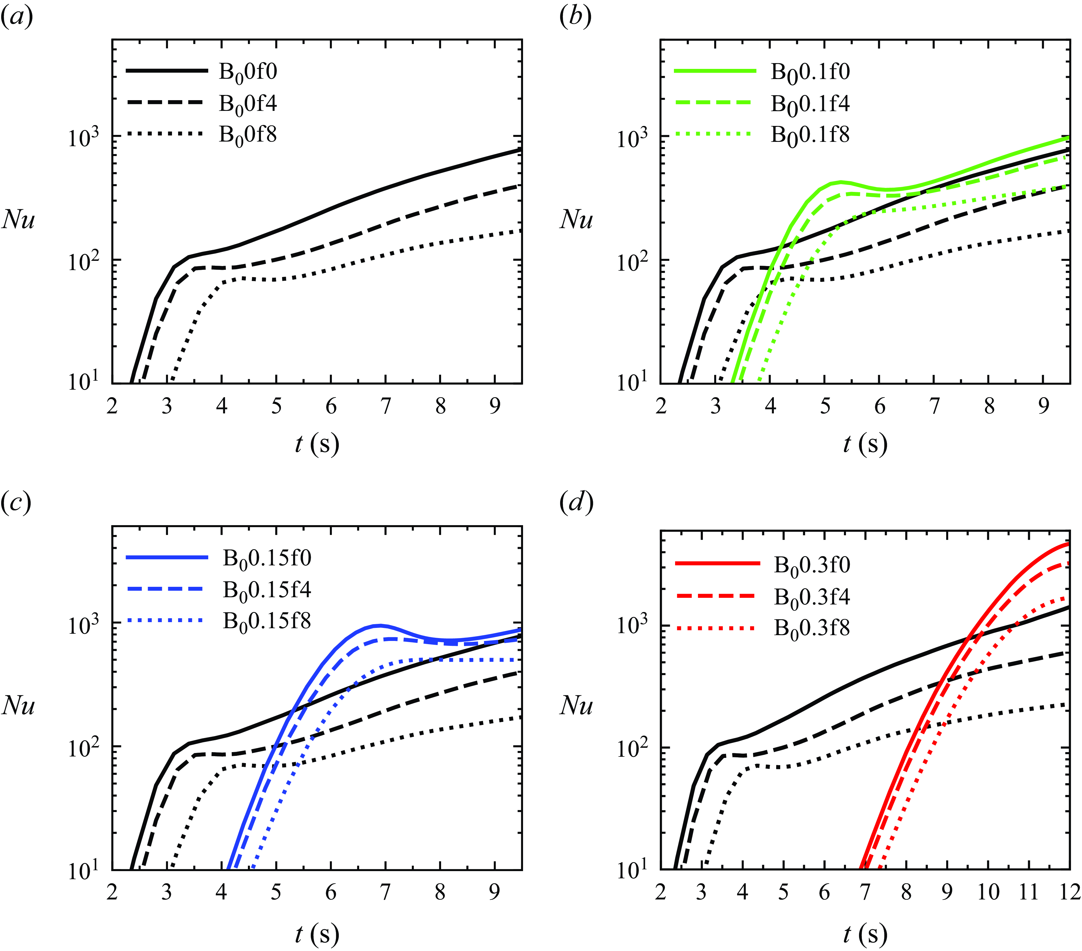
Temporal evolution of the Nusselt number (
 $Nu$
, defined in (2.8)) for non-rotating and rotating (a) HD cases, (b) HD and MHD for
 $B_0=0.1\,\mathrm {ms^{-1}}$
cases, (c) HD and MHD for
 $B_0=0.15\,\mathrm {ms^{-1}}$
cases, and (d) HD and MHD for
 $B_0=0.3\,\mathrm {ms^{-1}}$
cases.

3.5. Heat transport
In this subsection we quantify the heat transfer efficiency, measured by the Nusselt number (
 $Nu$
) (see (2.8)). We plot the
 $Nu$
, defined as the ratio of total heat transfer (convective and conductive) to conductive heat transfer, as a function of time in figure 8. Figure 8(a) depicts the temporal evolution of
 $Nu$
for the non-rotating and rotating HD cases. Figures 8(b), 8(c) and 8(d), respectively, compare the
 $Nu$
evolution between the HD cases and MHD cases for
 $B_0=0.1$
,
 $0.15$
and
 $0.3\,\mathrm {ms^{-1}}$
. The
 $Nu$
increases with the growth and subsequent turbulent mixing of the thermal plumes for all the cases. The effect of the Coriolis force on the damping of the growth of
 $h$
and fluctuations of vertical velocity (
 $u_3^{\prime }$
) and temperature (
 $T'$
), results in a decrease in heat transfer. Recall that the calculation of
 $Nu$
involves
 $\langle u_3^{\prime } T'\rangle$
(2.8), which reflects reversible exchanges between the hot and cold fluid. Briard et al. (Reference Briard, Gréa and Nguyen2024) suggested that the mixing parameter
 $\Theta$
(3.1) is highly correlated to the irreversible mixing. In figure 7(a) it has been observed that rotation in HD cases causes an enhancement in
 $\Theta$
indicating an increase in irreversible mixing and thereby decreasing reversible buoyancy flux
 $\langle u_3^{\prime } T'\rangle$
. Therefore, in the HD cases the
 $Nu$
decreases with an increase in rotation rates from
 $f=4$
to
 $8\,\mathrm {s^{-1}}$
compared to the non-rotating B
 $_0$
0f0 case (see figure 8
a). Similar results were also reported by Boffetta et al. (Reference Boffetta, Mazzino and Musacchio2016).
In the non-rotating MHD cases B
 $_0$
0.1f0 and B
 $_0$
0.15f0, the
 $Nu$
is enhanced compared to the corresponding HD case B
 $_0$
0f0 (figures 8
b and 8
c). The imposed
 $B_0$
delays the onset of instability, and therefore, we see a delay in the rapid increase in
 $Nu$
for the MHD cases. After this rapid increase, the
 $Nu$
decreases for some time while remaining larger than the HD case. We refer to this as the slowdown period, spanning
 $t\simeq$
5.25–6.25 s for B
 $_0$
0.1f0 (figure 8
b) and
 $t\simeq$
6.8–8.4 s for B
 $_0$
0.15f0 (figure 8
c). The Nusselt number
 $Nu$
then increases again, following a trend similar to that of the HD cases. The initial rapid growth and enhancement of
 $Nu$
before the slowdown period is caused by the unbroken vertically elongated plumes that grow without mixing, as indicated by the drop in
 $\Theta$
in figure 7
a, leading to an increase in reversible buoyancy flux
 $\langle u_3^{\prime } T'\rangle$
. This signifies that the elongated plumes are efficient in transferring heat between the bottom hot fluid and the upper cold fluid with limited mixing. The mushroom-shaped caps at the tips of elongated plumes undergo breakdown and detach from their respective plumes (see figure 4
c at
 $t\simeq 6.46, 7.51$
s for B
 $_0$
0.15f0), initiating irreversible mixing indicated by the subsequent rapid increase in
 $\Theta$
following its drop in figure 7(a). Consequently,
 $\langle u_3^{\prime } T'\rangle$
decreases, leading to a decrease in
 $Nu$
in the slowdown period. This decrease in
 $\langle u_3^{\prime } T'\rangle$
marks the transition from the initial regime of unbroken elongated plumes to the turbulent regime of broken small-scale structures, where
 $Nu$
begins to increase again. The
 $Nu$
remains higher than the corresponding HD case B
 $_0$
0f0 primarily due to the larger mixing layer height
 $h$
in the MHD cases B
 $_0$
0.1f0 and B
 $_0$
0.15f0 (figures 5
b and 5
c, respectively). The heat transfer enhancement (increase in
 $Nu$
) becomes more efficient as
 $B_0$
increases from
 $0.15$
to
 $0.3\,\mathrm {ms^{-1}}$
(compare figures 8
c and 8
d) due to the stronger vertical stretching of elongated plumes resulting in a significant increase in reversible buoyancy flux
 $\langle u_3^{\prime } T'\rangle$
until the transition to the turbulent regime, as well as the increase in mixing layer height. Note that in the MHD cases with
 $B_0=0.3$
, the flow has not reached a turbulent state by the end of simulations.
In the MHD cases, it has been observed that the increase in the strength of rotation causes an enhancement in mixing parameter
 $\Theta$
(irreversible) at the time of transition to turbulence compared to the non-rotating MHD case (see figure 7
a), causing a decrease in buoyancy flux
 $\langle u_3^{\prime } T'\rangle$
. Additionally, rotation dampens the growth of
 $h$
. Therefore, we observe a decrease in
 $Nu$
with increasing
 $f$
as compared to the corresponding non-rotating MHD cases (see figures 8
b, 8
c and 8
d). Note that the damping of
 $h$
primarily causes this decrease in
 $Nu$
in the turbulent regime. For B
 $_0$
0.1f4 and B
 $_0$
0.15f4,
 $Nu$
follows a trend similar to that of B
 $_0$
0.1f0 and B
 $_0$
0.15f0, respectively, in the sense that during the transition from initial regime to turbulent regime,
 $Nu$
first experiences a sudden drop then it slows down and approaches nearly a constant value before increasing again. However, in the B
 $_0$
0.1f8 and B
 $_0$
0.15f8 cases,
 $Nu$
does not experience a sudden drop during the slowdown. This behaviour is attributed to the stronger influence of the Coriolis force at
 $f=8\,\mathrm {s^{-1}}$
that results in a gradual breaking of the vertically stretched plumes instead of a sudden disintegration.
Interestingly, for all the rotating MHD cases (and in non-rotating ones), the
 $Nu$
remains higher than the corresponding rotating HD cases. This enhancement in
 $Nu$
is caused by the vertical stretching and collimation of flow structures along the vertical magnetic lines, which dampen the effect of rotation, reduce the mixing of fluids (
 $\Theta$
, see figure 7
a), thereby increasing
 $\langle u_3^{\prime } T'\rangle$
and
 $h$
. Note that the
 $Nu$
for the cases at
 $f=4,8\,\mathrm {s^{-1}}$
with
 $B_0=0.3\,\mathrm {ms^{-1}}$
is even higher than for the
 $B_0=0.1, 0.15\,\mathrm {ms^{-1}}$
cases at
 $f=0$
until the end of the simulations (compare figures 8
b, 8
c and 8
d). This is attributed to the relatively stronger vertical stretching of the plumes by
 $B_0=0.3\,\mathrm {ms^{-1}}$
. Therefore, even with stronger rotation rates (
 $f=8\,\mathrm {s^{-1}}$
), the heat transfer increases significantly at higher values of the vertically imposed mean magnetic field. This indicates that imposed magnetic fields can mitigate the instability-damping effects of rotation for efficient heat transfer.
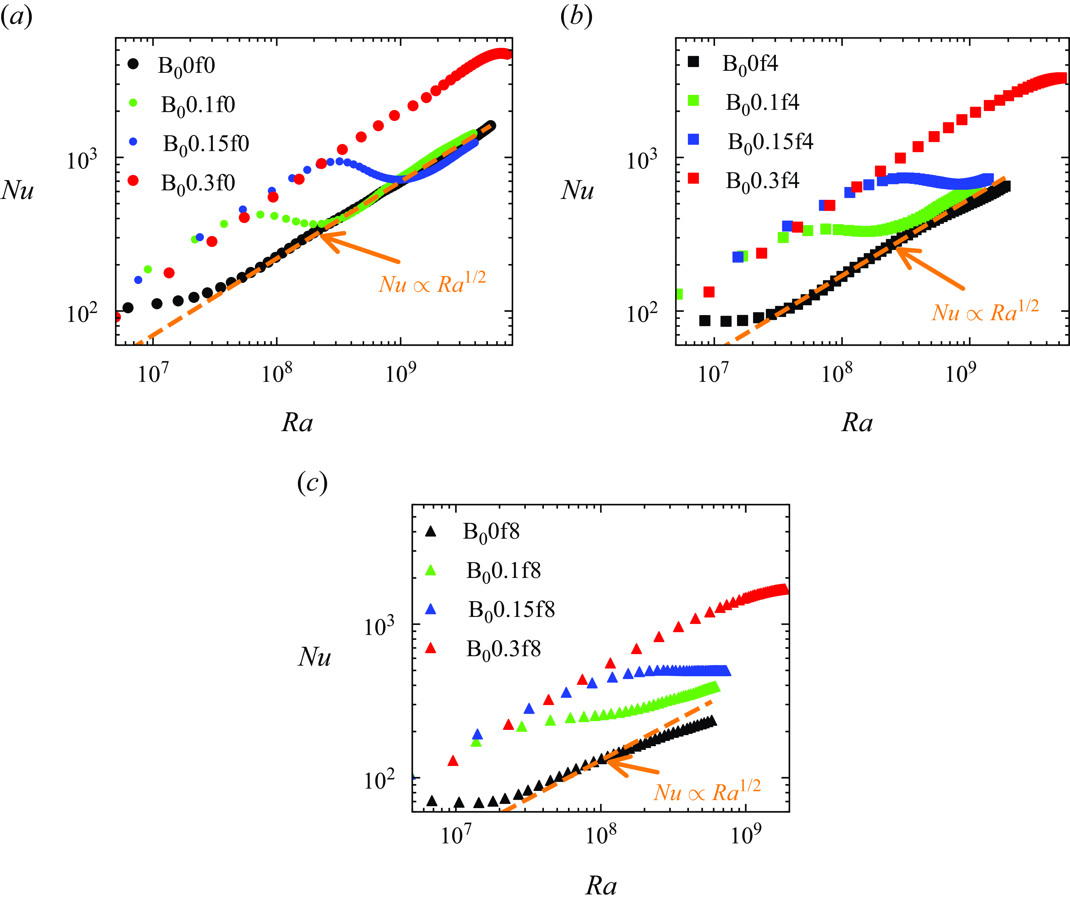
Variation of the Nusselt number,
 $Nu$
(defined in (2.8)), as a function of the Rayleigh number,
 $Ra$
(
 $\propto h^3$
), for the HD and MHD (a) non-rotating (
 $f=0$
), (b) rotating at
 $f=4\,\mathrm {s^{-1}}$
, and (c) rotating at
 $f=8\,\mathrm {s^{-1}}$
cases. Dashed orange lines represent the ultimate state predictions, i.e.
 $Nu \propto Ra^{1/2}$
scaling for
 $Pr=1$
(Boffetta et al. Reference Boffetta, Mazzino, Musacchio and Vozella2010b
,Reference Boffetta, Mazzino and Musacchio2016).

We further investigate the Nusselt number (
 $Nu$
) as a function of the Rayleigh number (
 $Ra$
), i.e. at a fixed
 $h$
, to clearly distinguish the mechanisms,
 $h$
or
 $\langle u_3^{\prime } T' \rangle$
, behind the enhancement in
 $Nu$
for the non-rotating and rotating MHD cases, and to assess the presence of the ultimate state scaling of thermal convection (
 $Nu \simeq Ra^{1/2} Pr^{1/2}$
) (Boffetta et al. Reference Boffetta, Mazzino, Musacchio and Vozella2010b
, Reference Boffetta, Mazzino and Musacchio2016). The
 $Ra$
is a dimensionless measure of the temperature difference that forces the system and is defined in terms of the mixing layer height
 $h$
as
 $Ra=\beta g \theta _0 h^3/ (\nu \kappa )$
(Boffetta et al. Reference Boffetta, Mazzino, Musacchio and Vozella2009, Reference Boffetta, Mazzino, Musacchio and Vozella2010b
). We plot
 $Nu$
as a function of
 $Ra$
in figures 9(a) 9(b) and 9(c) for the HD and MHD cases at
 $f=0$
, 4 and
 $8\,\mathrm {s^{-1}}$
, respectively. In figure 9(a) the significant enhancement in
 $Nu$
before the breakdown of plumes for the MHD cases compared to HD cases at
 $f=0$
is attributed to the increased buoyancy flux
 $\langle u_3^{\prime } T' \rangle$
, driven by vertically stretched plumes growing without mixing (
 $\Theta$
). After the plumes breakdown,
 $Nu$
decreases for B
 $_0$
0.1f0 and B
 $_0$
0.15f0 and becomes comparable to that of B
 $_0$
0f0. This signifies a decrease in buoyancy flux
 $\langle u_3^{\prime } T' \rangle$
as the mixing of fluids (
 $\Theta$
) begins. This further indicates the damping of the velocity fluctuations by the imposed
 $B_0$
in the turbulent regime (as shown later). In the turbulent regime of B
 $_0$
0.1f0 and B
 $_0$
0.15f0 cases,
 $Nu$
remains comparable to the HD case B
 $_0$
0f0 (figure 9
a), which verifies the argument made in the plots (figures 8
b and 8
c) of
 $Nu$
versus
 $t$
that the increase in
 $h$
primarily causes the heat transfer enhancement in the turbulent regime of non-rotating MHD cases compared to the non-rotating HD case. For the B
 $_0$
0.3f0 case,
 $Nu$
remains higher than the B
 $_0$
0f0, B
 $_0$
0.1f0 and B
 $_0$
0.15f0 cases due to strong vertical stretching of the elongated plumes without mixing and shows a small drop at
 $Ra\simeq 7{-}8\times 10^9$
due to the beginning of the plumes breakdown. In the presence of rotation at
 $f=4\,\mathrm {s^{-1}}$
and
 $f=8\,\mathrm {s^{-1}}$
, figures 9(b) and 9(c), respectively, demonstrate an enhancement of
 $Nu$
(or
 $\langle u_3^{\prime } T' \rangle$
) for the MHD cases over the HD case in both the initial and turbulent regimes. This signifies that the enhancement in heat transport (
 $Nu$
) in the rotating MHD cases relative to the corresponding HD cases is driven by both higher buoyancy flux and an increased mixing layer height (
 $h$
).
In figure 9(a), for HD case B
 $_0$
0f0 and MHD cases B
 $_0$
0.1f0 and B
 $_0$
0.15f0, our DNS confirms the presence of the ultimate state regime,
 $Nu \simeq Ra^{1/2} Pr^{1/2}$
. The
 $Pr=1$
for our simulations, and therefore
 $Nu \propto Ra^{1/2}$
which is similar to Boffetta et al. (Reference Boffetta, De Lillo, Mazzino and Vozella2012) and Boffetta & Mazzino (Reference Boffetta and Mazzino2017). The deviation from the ultimate state scaling (
 $Nu \propto Ra^{1/2}$
) can be observed in the rotating HD and MHD
 $B_0=0.1,0.15\,\mathrm {ms^{-1}}$
cases at
 $f=4,8\,\mathrm {s^{-1}}$
. Boffetta et al. (Reference Boffetta, Mazzino and Musacchio2016) and Wei et al. (Reference Wei, Li, Wang, Yang, Zhu, Qian and Luo2022) also reported a similar deviation from this scaling in the presence of rotation (HD) without a magnetic field. The ultimate state scaling is invalid for both the non-rotating and rotating MHD cases at
 $B_0=0.3\,\mathrm {ms^{-1}}$
because the flow is not in the turbulent regime.
3.6. Turbulent kinetic energy
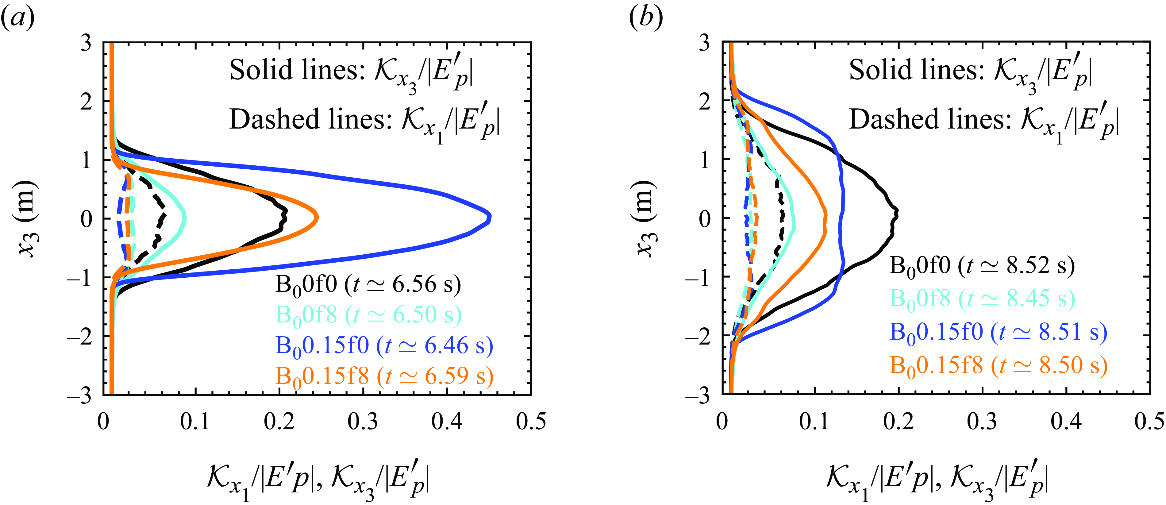
To further support the reasons for the enhancement of
 $Nu$
in the non-rotating and rotating MHD cases compared to the corresponding HD cases, as observed in the previous subsection (§ 3.5), we investigate the turbulent kinetic energy here. We plot the vertical profile of the horizontal (
 $x_1$
) and vertical (
 $x_3$
) components of the horizontally averaged turbulent kinetic energy (denoted by
 $\mathcal {K}$
), normalised by the released potential energy (
 $|E^\prime _p|$
), for the HD cases B
 $_0$
0f0 and B
 $_0$
0f8 and MHD cases B
 $_0$
0.15f0 and B
 $_0$
0.15f8 at
 $t\simeq 6.5$
s in figure 10(a) and at
 $t\simeq 8.5$
s in figure 10(b). The horizontal component of
 $\mathcal {K}$
(denoted by
 $\mathcal {K}_{x_1}$
) and vertical component of
 $\mathcal {K}$
(denoted by
 $\mathcal {K}_{x_3}$
) are defined as
 \begin{equation} \mathcal {K}_{x_1} = \frac { \overline {u_1{^{\prime }}^2}}{2}; \quad \mathcal {K}_{x_3} = \frac { \overline {u_3{^{\prime }}^2}}{2}, \end{equation}
where
 $\mathcal {K}_{x_1}$
and
 $\mathcal {K}_{x_3}$
are functions of
 $(x_3,t)$
. The potential energy released into the flow (
 $E^\prime _p$
) at any time instant (
 $t$
) is computed as (Cook et al. Reference Cook, Cabot and Miller2004; Briard et al. Reference Briard, Gréa and Nguyen2024)
 \begin{equation} E^\prime _p (t) = E_p(t) - E_p(0), \end{equation}
where the potential energy (
 $E_p$
) is defined as (Boffetta & Mazzino Reference Boffetta and Mazzino2017)
 \begin{equation} E_p = -\beta g \langle x_3 T\rangle . \end{equation}
For all cases, figures 10(a) and 10(b) demonstrate the dominance of
 $\mathcal {K}_{x_3}$
over
 $\mathcal {K}_{x_1}$
, indicating that the flow is primarily driven in the vertical direction, as expected due to vertically downward acting gravity normal to the interface. Figure 10(a) at
 $t\simeq 6.5$
s shows that
 $\mathcal {K}_{x_3}$
is significantly smaller for B
 $_0$
0f8 than that for B
 $_0$
0f0 due to the presence of the Coriolis force, resulting in smaller
 $Nu$
for the former case compared to the latter. For B
 $_0$
0.15f0 and B
 $_0$
0.15f8,
 $\mathcal {K}_{x_3}$
is significantly larger than the corresponding
 $\mathcal {K}_{x_1}$
. This signifies that in the presence of an imposed magnetic field, the elongated plumes exhibit higher fluctuations in vertical velocity with limited horizontal interactions between the plumes. Therefore, the elongated plumes are efficient in transferring heat between two fluids. The higher
 $\mathcal {K}_{x_3}$
in the MHD cases B
 $_0$
0.15f0 and B
 $_0$
0.15f8 compared to the corresponding HD cases B
 $_0$
0f0 and B
 $_0$
0f8 implies an enhancement in
 $Nu$
for the MHD cases. For the HD case B
 $_0$
0f0,
 $\mathcal {K}_{x_3}$
is higher than
 $\mathcal {K}_{x_1}$
, but
 $\mathcal {K}_{x_1}$
exhibits significantly larger values compared to the MHD B
 $_0$
0.15f0 and B
 $_0$
0.15f8 cases. This indicates relatively stronger horizontal interactions between the flow structures in B
 $_0$
0f0 than in B
 $_0$
0.15f0 and B
 $_0$
0.15f8 because the flow is in the turbulent state in B
 $_0$
0f0 at
 $t\simeq 6.5$
s.
Vertical profiles of the horizontal (
 $x_1$
) and vertical (
 $x_3$
) components of horizontally averaged turbulent kinetic energy (denoted by
 $\mathcal {K}_{x_1}$
and
 $\mathcal {K}_{x_3}$
, respectively), normalised by the released potential energy
 $|E^\prime _p|$
(defined in (3.4)), for the HD cases B
 $_0$
0f0 and B
 $_0$
0f8, and MHD cases B
 $_0$
0.15f0 and B
 $_0$
0.15f8 at time (a)
 $t\simeq 6.5$
s and (b)
 $t\simeq 8.5$
s. Solid lines denote
 $\mathcal {K}_{x_3}/|E^\prime _p|$
, while dashed lines denote
 $\mathcal {K}_{x_1}/|E^\prime _p|$
.

Figure 10(b) depicts that at
 $t\simeq 8.5$
s, for B
 $_0$
0.15f0, the
 $\mathcal {K}_{x_3}$
is smaller near the mid-plane (
 $x_3=0$
) compared to the B
 $_0$
0f0 case. However, towards the plume tips (
 $x_3\simeq \pm 1.5$
m) the
 $\mathcal {K}_{x_3}$
for B
 $_0$
0.15f0 is higher compared to B
 $_0$
0f0 indicating a wider mixing layer height
 $h$
for B
 $_0$
0.15f0, as also evident from figure 5(c). Since
 $Nu$
also depends on
 $h$
(see (2.8)), the
 $Nu$
is higher for B
 $_0$
0.15f0 than the B
 $_0$
0f0 case in the turbulent regime primarily as a consequence of the increased
 $h$
. The comparison between figures 10(a) and 10(b) reveals that
 $\mathcal {K}_{x_3}$
is reduced at
 $t\simeq 8.5$
s (turbulent regime) compared to that at
 $t\simeq 6.5$
s (beginning of the plumes breakdown) for the MHD case B
 $_0$
0.15f0, and this reduction is small for B
 $_0$
0.15f8. Therefore, the imposed
 $B_0$
dampens the velocity fluctuations in the turbulent regime. Consequently, a decrease in
 $Nu$
after the plumes breakdown was observed for the MHD cases in figures 9(a), 9(b) and 9(c), where
 $Nu$
is plotted as a function of
 $Ra(\propto h^3)$
. Although, for the B
 $_0$
0.15f8 case, the reduction in
 $\mathcal {K}_{x_3}$
is small, it remains higher and spans over a wider mixing layer (
 $h$
) than the corresponding HD case. Owing to this, the
 $Nu$
is enhanced both as a function of time and
 $Ra(\propto h^3)$
in the turbulent regime of the rotating MHD cases as compared to the corresponding HD cases, as observed in figures 8(b), 8(c), 8(d), 9(b) and 9(c). In figure 10(b) we can observe the smaller
 $\mathcal {K}_{x_3}$
for B
 $_0$
0.15f8 as compared to B
 $_0$
0.15f0 signifying weaker turbulence in the rotating MHD case relative to the non-rotating MHD case. This also corroborates the smaller
 $Nu$
in the rotating MHD case (B
 $_0$
0.15f8) compared to the non-rotating MHD case (B
 $_0$
0.15f0).
3.7. Force balance
From the above discussion, it is apparent that the thermal plumes’ formation, evolution and disintegration under the influence of rotation and imposed magnetic field drive the heat transfer phenomenon. Therefore, in this subsection we analyse the dynamic balance between the different forces to understand the behaviour of these thermal plumes. We calculate the horizontally averaged
 $\textit{r.m.s.}$
(using (2.6)) of each force i.e. the inertia (
 $\boldsymbol {F}_{\!I}$
), the advection (
 $\boldsymbol {F}_{\!A}$
), the pressure gradient (
 $\boldsymbol {F}_{\!P}$
), the Coriolis (
 $\boldsymbol {F}_{\!C}$
), the Lorentz (
 $\boldsymbol {F}_{\!L}$
), the buoyancy (
 $\boldsymbol {F}_{\!B}$
) and the viscous (
 $\boldsymbol {F}_{\!V}$
), in momentum equation (2.1b
) (Guzmán et al. Reference Aguirre Guzmán, Madonia, Cheng, Ostilla-Mónico, Clercx and Kunnen2021; Naskar & Pal Reference Naskar and Pal2022 a
,Reference Naskar and Pal
b
). We also define the
 $\textit{r.m.s.}$
horizontal forces as
 $F_{x_1x_2,\,r.m.s.}= (F_{x_1,\,r.m.s.}^2+F_{x_2,\,r.m.s.}^2 )^{1/2}$
, where
 $F_{x_1,\,r.m.s.}$
and
 $F_{x_2,\,r.m.s.}$
denote the components of any
 $\textit{r.m.s.}$
force in the
 $x_1$
and
 $x_2$
directions. The Lorentz force exerted by the magnetic field acts in all three directions, the Coriolis force, due to rotation about the vertical axis, acts only in the horizontal directions, and the buoyancy force is purely vertical due to the gravity vector.
Instantaneous vertical profiles of the horizontally averaged r.m.s. of each term (force) present in the vertical and horizontal component of the momentum equation (2.1b
). Horizontal forces,
 $F_{x_1x_2,\textit{r.m.s.}}=\sqrt {F_{x_1,\textit{r.m.s.}}^2+F_{x_2,\textit{r.m.s.}}^2}$
, are shown with dashed lines, whereas the vertical forces,
 $F_{x_3,\textit{r.m.s.}}$
, are indicated with solid lines for (a) the non-rotating MHD case B
 $_0$
0.15f0 at
 $t\simeq 6.46$
s,
 $7.51$
s, (b) the rotating MHD case B
 $_0$
0.15f4 at
 $t\simeq 6.6$
s,
 $7.55$
s, and (a) the rotating MHD case B
 $_0$
0.15f8 at
 $t\simeq 6.58$
s,
 $7.51$
s.

The instantaneous vertical (
 $x_3$
) variation of
 $\textit{r.m.s.}$
horizontal
 $F_{x_1x_2,\,r.m.s.}$
and
 $\textit{r.m.s.}$
vertical
 $F_{x_3,\,r.m.s.}$
forces for the MHD cases B
 $_0$
0.15f0, B
 $_0$
0.15f4 and B
 $_0$
0.15f8 is illustrated in figures 11(a), 11(b) and 11(c), respectively, at time instants
 $t\simeq 6.5$
s and
 $t\simeq 7.5$
s. These time instants correspond to the breakdown of plumes, which were depicted in figures 4(c) and 4(d) for the cases B
 $_0$
0.15f0 and B
 $_0$
0.15f8. We first recall that initially at
 $t=0$
s, the fluids are at rest (i.e.
 $\boldsymbol {u}(\boldsymbol {x},t)=0$
), and the mean magnetic field
 $B_0$
is imposed vertically. The random perturbations are seeded into the temperature field, which induces velocity fluctuations via the buoyancy term
 $\beta g T \delta _{i3}$
in the momentum equation (2.1b
). These velocity fluctuations generate magnetic field fluctuations (
 $\boldsymbol {B}'$
) through the stretching term
 $B_0 \partial u_i/\partial x_j$
in the induction equation (2.1d
). Subsequently, the Lorentz force due to the total magnetic field (
 $B_i=B_0\delta _{i3}+B_i'$
) present as a source term in momentum equation (2.1b
), alters the flow evolution, which in turn modifies the production of
 $\boldsymbol {B}'$
in the induction equation. This phenomenon repeats at successive time steps. The
 $r.m.s.$
of the Lorentz force includes a combined contribution from the mean and fluctuating components of the magnetic field. Since only the mean magnetic field is imposed vertically (
 $B_0$
), the vertical component of the Lorentz force is expected to be higher than its horizontal components until the fluctuating magnetic field becomes significant due to the breakdown of flow structures. Therefore, the horizontal component of the Lorentz force acts to break the plumes.
Figure 11(a) for the B
 $_0$
0.15f0 case at
 $t\simeq 6.46$
s shows that the vertical component (solid line) of the Lorentz force is higher than the horizontal component (dashed line), signifying that the stretching of plumes is stronger than their breakup (see temperature contours in figure 4(c) at
 $t\simeq 6.46$
s). The strength of the horizontal component of the Lorentz force is slightly higher towards the tips of plumes (i.e.
 $x_3\simeq \pm 1$
m) than towards the centre or mid-plane (at
 $x_3\simeq 0$
m), indicating that more breakup of elongated plumes occurs at their tips. Consequently, the larger nonlinear interactions near the plume tips result in a significantly higher advection force, which becomes the dominant force among all forces, at the plume tips compared to near the mid-plane. The magnitude of the inertial and pressure forces is also greater at the plume tips than at the mid-plane. In contrast to the Lorentz, advection, inertia and viscous forces, the buoyancy force is larger towards the mid-plane than at the plume tips. At
 $t\simeq 7.51$
s in figure 11(a), the horizontal component of the Lorentz force is higher than the vertical component, and both components increase towards the mid-plane, resulting in the breakup of each plume along its entire surface (see temperature contours in figure 4(c) at
 $t\simeq 7.51$
s and supplementary movie 3). Therefore, the advection force also increases towards the mid-plane while spanning over the entire height of the mixing layer. The horizontal components of the advection and the pressure forces are also higher than the corresponding vertical components. The magnitudes of the Lorentz and advection forces are higher at
 $t\simeq 7.51$
s than at
 $t\simeq 6.46$
s owing to the increased breakup of the plumes.
At
 $t\simeq 6.6$
s for the rotating MHD case B
 $_0$
0.15f4, figure 11(b) shows competition between the Coriolis and Lorentz forces. The Coriolis force and the horizontal Lorentz force are in close balance near the mid-plane, while the Coriolis force dominates over the horizontal Lorentz force close to the plume tips. Therefore, the breakup of elongated plumes due to the horizontal Lorentz force is inhibited by the Coriolis force. Additionally, the Coriolis force is smaller than the vertical Lorentz force at the mid-plane, while it dominates near the plume tips. Therefore, the growth of the plumes due to the vertical stretching caused by the vertical Lorentz force is damped by the Coriolis force, as observed in the plot for the temporal evolution of the mixing layer height
 $h$
in figure 5(c). The higher values of the vertical component of the Lorentz force than its horizontal component indicate that the vertical stretching of the plumes prevails over the plume breakup at
 $t\simeq 6.6$
s. As a result, the vertical component of the advection, inertial, and viscous forces remain higher than their horizontal counterparts. In contrast, the horizontal component of the pressure force is higher than its vertical component. At
 $t\simeq 7.55$
s, both the horizontal and the vertical components of the Lorentz force dominate over the Coriolis force, except near the plume tips. This signifies that the effect of the Coriolis force in inhibiting the growth and breakup of the plumes, except near the plume tips, is mitigated. The magnitude of the horizontal and vertical components of the advection force are comparable.
In figure 11(c) for the high rotation rate case B
 $_0$
0.15f8 at
 $t\simeq 6.58$
s, the Coriolis force dominates significantly over the horizontal and vertical components of the Lorentz force, which greatly inhibits the growth and breakdown of the plumes (see temperature contours in figure 4(d) at
 $t\simeq 6.58$
s and supplementary movie 4). The horizontal component of the pressure force also increases significantly compared to its vertical component. At
 $t\simeq 7.51$
s, the horizontal component of the Lorentz force is greater than its vertical component, suggesting that the breakdown is prominent over the vertical stretching of the plumes. However, the breakdown is still retarded by the dominant Coriolis force. Therefore, the vertical plumes with less distortion are visible in figure 4(d) at
 $t\simeq 7.51$
s. We can conclude that with an increase in rotation rates (B
 $_0$
0.15f4 and B
 $_0$
0.15f8), the Coriolis force becomes stronger and dominates significantly over the Lorentz force at high rotation (B
 $_0$
0.15f8), resulting in the damping of the plumes growth and breakup. As a result, the advection force is reduced with increasing rotation rates compared to the non-rotating case B
 $_0$
0.15f0, which can be observed by comparing figures 11(a), 11(b) and 11(c) for B
 $_0$
0.15f0, B
 $_0$
0.15f4 and B
 $_0$
0.15f8, respectively, at
 $t\simeq 6.5$
s,
 $7.5$
s. This reduction in advection force causes a decrease in heat transfer, which corroborates the decrease in
 $Nu$
, observed in figure 8c, in the B
 $_0$
0.15f4 and B
 $_0$
0.15f8 cases compared to B
 $_0$
0.15f0.
Instantaneous vertical profiles of the resultant
 $\textit{r.m.s.}$
values of each force
 $(F_{\textit{r.m.s.}}=\sqrt {F_{x_1,\textit{r.m.s.}}^2+F_{x_2,\textit{r.m.s.}}^2+F_{x_3,\textit{r.m.s.}}^2})$
in momentum equation (2.1b
) for the rotating (a) HD case B
 $_0$
0f4 at
 $t\simeq 6.62$
s,
 $7.52$
s, (b) HD case B
 $_0$
0f8 at
 $t\simeq 6.73$
s,
 $7.63$
s, and (c) MHD case B
 $_0$
0.15f8 at
 $t\simeq 6.58$
s,
 $7.51$
s. Solid lines of different colours represent the resultant r.m.s. values of the corresponding force. The dashed blue line denotes the horizontal Coriolis force.

The vertical variation of the resultant r.m.s. values of each force, computed as
 $F_{r.m.s.}= (F_{x_1,\,r.m.s.}^2+F_{x_2,\,r.m.s.}^2+F_{x_3,\,r.m.s.}^2 )^{1/2}$
, in the momentum equation (2.1b
) for the rotating HD cases B
 $_0$
0f4, B
 $_0$
0f8, and MHD case B
 $_0$
0.15f8 is shown in figure 12(a), 12(b) and 12(c), respectively, at two different time instants. The deviations from the geostrophic balance between the Coriolis and pressure forces are measured by the ageostrophy and is estimated as the difference between these two forces. Figures 12(a) and 12(b) for the HD cases illustrate that at a rotation rate of
 $f=4\,\mathrm {s^{-1}}$
(B
 $_0$
0f4 case) the ageostrophy is higher, but it reduces significantly when the rotation rate increases to
 $f=8\,\mathrm {s^{-1}}$
(B
 $_0$
0f8 case). This signifies that the Coriolis and pressure forces are in close balance in B
 $_0$
0f8. This confirms the presence of the Taylor–Proudman constraint, which results in the vertical alignment of the flow structures as observed in the temperature contours in figure 4(b). Boffetta et al. (Reference Boffetta, Mazzino and Musacchio2016) also reported the existence of the Taylor–Proudman constraint in the rotating RT instability from flow visualisation. In the B
 $_0$
0f4 case the Coriolis and pressure forces are the subdominant forces, whereas they become nearly dominant forces among all forces in the B
 $_0$
0f8 case. Therefore, we expect the leading-order geostrophic balance between the Coriolis and pressure forces to occur at rotation rates of
 $f\gt 8\,\mathrm {s^{-1}}$
, constraining the flow to be 2-D satisfying the Taylor–Proudman theorem.
For the rotating MHD case B
 $_0$
0.15f8 in figure 12(c) at
 $t\simeq 6.58$
s and
 $t\simeq 7.51$
s, the ageostrophy is higher than the corresponding HD case B
 $_0$
0f8 (figure 12
b). This deviation from the geostrophic balance is attributed to the presence of the Lorentz force. Additionally, in the B
 $_0$
0.15f8 case the higher ageostrophy at
 $t\simeq 7.51$
s compared to that at
 $t\simeq 6.58$
s due to the increase in the Lorentz force indicates that the deviation from the geostrophic balance increases as the RT instability grows. Therefore, in contrast to the rotating HD case, the geostrophic balance is not expected at high rotation rates in the MHD cases owing to the mitigation of the effect of the Coriolis force by the Lorentz force. Due to this mitigation of the Coriolis force effect, the advection force at
 $t\simeq 7.51$
s in the B
 $_0$
0.15f8 case (figure 12
c) is higher than in the B
 $_0$
0f8 case at
 $t\simeq 7.63$
s (figure 12
b). This results in efficient heat transfer in the rotating MHD B
 $_0$
0.15f8 case compared to the rotating HD B
 $_0$
0f8 case.
3.8. Energy budget
The above analysis reveals that the Coriolis and Lorentz forces significantly impact the growth and breakdown of thermal plumes into small-scale turbulence. Since small-scale turbulence significantly alters the heat transfer phenomenon, we evaluate the turbulent energetics associated with the flow in this subsection to understand the generation and evolution of turbulent kinetic energy in the presence of the imposed magnetic field and rotation. The temporal evolution equation of the horizontally averaged turbulent kinetic energy,
 $\mathcal {K}=\overline {u_i'u_i'}/2$
is given as follows:
 \begin{equation} \frac {{\rm d}\mathcal {K}}{{\rm d}t}=\mathcal {B}-\epsilon _v+\mathcal {S}+\mathcal {P}-\frac {\partial \mathcal {T}_j}{\partial x_j}. \end{equation}
Here, the buoyancy flux
 \begin{equation} \mathcal {B}=\beta g \overline {u_3^{\prime }T'} \end{equation}
represents the conversion of available potential energy into
 $\mathcal {K}$
. The viscous dissipation rate
 \begin{equation} \epsilon _v=2\nu \overline { s_{ij}' s_{ij}'} \, ; \quad s_{ij}'=\frac {1}{2}\left ( \frac {\partial u_i'}{\partial x_j} + \frac {\partial u_j'}{\partial x_i} \right ), \end{equation}
acts as a sink for
 $\mathcal {K}$
that converts the
 $\mathcal {K}$
to internal energy. The shear production rate of
 $\mathcal {K}$
,
 \begin{equation} \mathcal {S}=- \overline {u_i' u_j'} \frac {\partial \overline {u_i}}{ \partial x_j} \end{equation}
is negligible since no mean velocity field is involved in the present study. The production of
 $\mathcal {K}$
due to the work done by the Lorentz force on the velocity field is (Naskar & Pal Reference Naskar and Pal2022b
)
 \begin{equation} \mathcal {P}= \mathcal {P}_1 +\mathcal {P}_2+ \mathcal {P}_3, \end{equation}
where
 \begin{equation} \mathcal {P}_1=-\overline {B_j}\,\overline {B_i'\frac {\partial u_i'}{\partial x_j}}, \quad \mathcal {P}_2=\overline {u_i'B_j'}\,\frac {\partial \overline {B_i}}{\partial x_j} , \quad \mathcal {P}_3=-\overline {B_i'B_j'\frac {\partial u_i'}{\partial x_j}}. \end{equation}
The energy exchange between the velocity and the magnetic fields occurs through the magnetic production terms
 $\mathcal {P}_1$
,
 $\mathcal {P}_2$
and
 $\mathcal {P}_3$
. The transport of
 $\mathcal {K}$
, which represents the divergence of
 $\mathcal {K}$
flux
 $\mathcal {T}_j$
,
 \begin{equation} \frac {\partial \mathcal {T}_j}{\partial x_j} = \frac {\partial }{\partial x_j} \left (\overline { p' u_j' } - 2\nu \overline { s_{ij}' u_i' } + \frac {1}{2}\overline { u_i' u_i' u_j'} - \overline {u_i'B_i'B_j'} - \overline {B_j}\,\overline {u_i'B_i'} \right ) \end{equation}
becomes negligible when integrated vertically (
 $x_3$
). The time evolution of the vertically (
 $x_3$
) integrated
 $\mathcal {K}$
budget terms of (3.6) are depicted in figures 13(a), 13(b), 13(c) and 13(d) for the non-rotating HD case B
 $_0$
0f0, non-rotating MHD case B
 $_0$
0.1f0, rotating MHD case B
 $_0$
0.1f8 and non-rotating MHD case B
 $_0$
0.15f0, respectively. In the B
 $_0$
0f0 case the buoyancy flux (
 $\mathcal {B}$
), which produces
 $\mathcal {K}$
, together with the viscous dissipation rate (
 $\epsilon _v$
) balances
 ${{\rm d}\mathcal {K}}/{{\rm d}t}$
(see figure 13
a). In the MHD B
 $_0$
0.1f0, B
 $_0$
0.1f8 and B
 $_0$
0.15f0 cases, a negative value of the term
 $\mathcal {P}$
signifies that the energy is transferred from the velocity field to the magnetic field (figures 13
b, 13
c and 13
d). Therefore, the term
 $\mathcal {P}$
acts as a sink for the
 $\mathcal {K}$
, which converts the turbulent kinetic energy to turbulent magnetic energy. In the MHD cases,
 $\mathcal {B}$
together with
 $\mathcal {P}$
and
 $\epsilon _v$
balances
 ${{\rm d}\mathcal {K}}/{{\rm d}t}$
. We obtain the
 $\mathcal {K}$
budget closure in all simulation cases, indicating that the grid spacing considered in the present simulations is adequate to capture the small-scale turbulence. The comparison of figures 13(b) and 13(c) for the B
 $_0$
0.1f0 and B
 $_0$
0.1f8 cases, respectively, shows that the magnitude of all the budget terms (
 ${{\rm d}\mathcal {K}}/{{\rm d}t}$
,
 $\mathcal {B}$
,
 $\epsilon _v$
and
 $\mathcal {P}$
) is reduced in B
 $_0$
0.1f8 compared to B
 $_0$
0.1f0 owing to the instability-damping effects of the Coriolis force.
Temporal evolution of vertically (
 $x_3$
) integrated turbulent kinetic energy (
 $\mathcal {K}$
) budget terms of (3.6) for the (a) non-rotating HD case B
 $_0$
0f0, (b) non-rotating MHD case B
 $_0$
0.1f0, (c) rotating MHD case B
 $_0$
0.1f8, and (d) non-rotating MHD case B
 $_0$
0.15f0.

To quantify the influence of the imposed magnetic field and rotation on the conversion of the turbulent kinetic energy to turbulent magnetic energy, we plot the ratio
 $R=\mathcal {M}/\mathcal {K}$
, where
 $\mathcal {K}=\overline {u_i'u_i'}/2$
and
 $\mathcal {M}=\overline {B_i'B_i'}/2$
represent the horizontally averaged turbulent kinetic and magnetic energies as a function of time in figure 14 for both non-rotating and rotating MHD cases with
 $B_0=0.1,0.15\,\mathrm {ms^{-1}}$
. Here, the ratio
 $R$
is computed by vertically (
 $x_3$
) integrating
 $\mathcal {M}$
and
 $\mathcal {K}$
. In all cases,
 $R\lt 1$
throughout the flow evolution, which shows that the production of
 $\mathcal {K}$
remains higher than
 $\mathcal {M}$
. In the absence of rotation, we observe that with an increase in
 $B_0$
from 0.1 to
 $0.15\,\mathrm {ms^{-1}}$
,
 $\mathcal {M}$
increases, whereas
 $\mathcal {K}$
decreases in the asymptotic state. Consequently, the increase in the ratio
 $\mathcal {M}/\mathcal {K}$
with
 $B_0$
is apparent in the asymptotic state in figure 14. Briard et al. (Reference Briard, Gréa and Nguyen2024) also observed a similar increase in the ratio
 $\mathcal {M}/\mathcal {K}$
with increasing
 $B_0$
. In the rotating MHD cases, the increasing strength of the Coriolis force damps the production of both
 $\mathcal {K}$
and
 $\mathcal {M}$
compared to the non-rotating cases. The increase in the ratio
 $\mathcal {M}/\mathcal {K}$
with increasing
 $f$
(
 $4$
to
 $8\,\mathrm {s^{-1}}$
) for both
 $B_0 = 0.1$
and
 $0.15\,\mathrm {ms^{-1}}$
at the end of the simulations indicates that the production of
 $\mathcal {M}$
relative to
 $\mathcal {K}$
is higher in rotating MHD compared to non-rotating cases.
Time evolution of the turbulent magnetic to kinetic energy ratio
 $R=\mathcal {M}/\mathcal {K}$
for the non-rotating and rotating MHD cases with
 $B_0=0.1$
and
 $0.15\,\mathrm {ms^{-1}}$
.

4. Conclusions
We have conducted DNS to investigate the thermal convection driven by the RT instability under the combined influence of the externally imposed vertical mean magnetic field
 $B_0$
(scaled as the Alfvèn velocity) and rotation about the vertical axis. The RT instability in the simultaneous presence of the magnetic field and rotation plays a crucial role in astrophysical phenomena such as solar prominences (Hillier Reference Hillier2017), acceleration at the disc-magnetosphere boundary (Kulkarni & Romanova Reference Kulkarni and Romanova2008) and many more. It can also be important in engineering applications such as ICF implosions (Zhou Reference Zhou2017; Walsh & Clark Reference Walsh and Clark2021
Reference Walsh and Clark
a
; Zhou et al. Reference Zhou, Sadler and Hurricane2024). Our motivation for this investigation emanates from the absence of any study on the combined influence of the magnetic field and rotation on the evolution of RT instability in the literature. Our DNS provides a comprehensive view of how the interplay between the vertical mean magnetic field and rotation affects the formation and breakup of flow structures and the heat transfer efficiency in the RT configuration. The present simulations can be used as a framework to gain important insights into the engineering and astrophysical phenomena discussed above.
We perform the simulations for
 $B_0=0$
,
 $0.1$
,
 $0.15$
and
 $0.3\,\mathrm {ms^{-1}}$
each at Coriolis frequencies of
 $f=0$
,
 $4$
and
 $8\,\mathrm {s^{-1}}$
. In rotating HD cases (
 $B_0=0$
), with increasing strength of rotation, the Coriolis force stabilises the flow by inhibiting the formation of the mushroom-shaped caps at the plume tips and the deformation of plumes, leading to the appearance of coherent vertical plumes in the turbulent regime. Consequently, rotation enhances molecular mixing between the fluids, quantified using the mixing parameter
 $\Theta$
, which dampens the growth rate (
 $\alpha$
) of the mixing layer height
 $h$
and the turbulent velocity fluctuations compared to the non-rotating HD case. A slight delay in the onset of RT instability is observed at
 $f=8\,\mathrm {s^{-1}}$
compared to the
 $f=0$
case. In the presence of the imposed
 $B_0$
at
 $f=0$
, smooth vertically elongated plumes form owing to the suppression of the secondary shear instabilities at small scales, which inhibits horizontal plume interactions, resulting in the rapid growth of
 $h$
. Later, these plumes become unstable, leading to the appearance of mushroom-shaped caps at their tips. Eventually, these thin plumes completely disintegrate into small structures due to the continuous vertical stretching by
 $B_0$
, and the flow becomes turbulent. The turbulence remains weaker than the corresponding HD case due to the collimation of fluid structures along the vertical magnetic field lines. Therefore, an enhancement in the mixing layer height
 $h$
is observed compared to the HD cases. We find that the delay in the onset of RT instability increases with an increase in
 $B_0$
compared to the non-rotating HD case, consistent with the previously developed linear theory. Additionally, the flow collimation along the vertical magnetic field lines becomes stronger with an increase in
 $B_0$
, enhancing
 $h$
. With the inclusion of a high rotation rate of
 $f=8\,\mathrm {s^{-1}}$
along with
 $B_0$
, the Coriolis force inhibits the formation of mushroom-shaped caps at the plume tips and dampens the growth of vertically elongated plumes and
 $h$
, as compared to the corresponding non-rotating MHD case. The breakdown of plumes into small-scale turbulence due to the continued vertical stretching by
 $B_0$
is also dampened by the Coriolis force. We find that the tendency of the Coriolis force to inhibit the growth of
 $h$
increases with an increase in
 $f(=4,8\,\mathrm {s^{-1}})$
for each
 $B_0$
. In the asymptotic state, the Coriolis force tends to reduce mixing between the fluids in MHD cases compared to non-rotating MHD cases, unlike in rotating HD cases where it substantially enhances mixing. Consequently, the damping of the growth rate (
 $\alpha$
) of the mixing layer height due to rotation is less pronounced in the rotating MHD cases compared to the corresponding rotating HD cases. Additionally, increasing
 $B_0$
from
 $0.1$
to
 $0.15\,\mathrm {ms^{-1}}$
further reduces the dampening of
 $\alpha$
in the rotating MHD cases, signifying that the vertical mean magnetic field mitigates the Coriolis force’s instability-damping effect.
The Nusselt number
 $Nu$
, quantifying the heat transfer efficiency, is calculated based on
 $h$
and the reversible buoyancy flux
 $\langle u_3^{\prime } T'\rangle$
, where
 $u_3^{\prime }$
and
 $T^{\prime }$
represent the fluctuating vertical velocity and temperature. The
 $Nu$
is analysed both as a function of time and Rayleigh number (
 $Ra (\propto h^3$
)), i.e. at a fixed
 $h$
. We observe that in the HD cases, heat transport (
 $Nu$
) decreases as a function of time and
 $Ra$
as the strength of rotation increases from
 $f=4$
to
 $8\,\mathrm {s^{-1}}$
compared to
 $f=0$
due to the enhanced mixing (
 $\Theta$
) of fluids, which dampens
 $\langle u_3^{\prime } T'\rangle$
and
 $h$
. In the non-rotating MHD cases with
 $B_0 = 0.1,0.15\,\mathrm {ms^{-1}}$
, heat transport is more efficient than in the non-rotating HD cases. This enhancement in heat transfer during the initial regime of unbroken elongated plumes is primarily caused by the vertical stretching of the plumes with limited mixing, leading to an increase in reversible exchanges between the fluids (
 $\langle u_3^{\prime } T'\rangle$
). This signifies that elongated plumes are efficient in transporting heat between hot and cold fluids with limited mixing. However, in the turbulent regime,
 $u_3^{\prime }$
and
 $\langle u_3^{\prime } T'\rangle$
are dampened by
 $B_0$
, and the heat transfer enhancement is mainly attributed to the collimation of the flow structures along the vertical magnetic field lines, resulting in increased
 $h$
compared to the non-rotating HD case. With the addition of rotation to
 $B_0(=0.1,0.15\,\mathrm {ms^{-1}})$
, heat transport (
 $Nu$
) reduces in both the initial and turbulent regimes as
 $f(=4,8\,\mathrm {s^{-1}})$
increases, compared to the corresponding non-rotating MHD cases, due to the Coriolis force’s instability-damping effect. We find that the enhancement in heat transfer increases significantly when the strength of the imposed
 $B_0$
becomes stronger (
 $B_0=0.3\,\mathrm {ms^{-1}}$
) in both the non-rotating and rotating scenarios. Interestingly, in rotating MHD cases, heat transport is more efficient compared to the corresponding rotating HD cases, due to the effect of
 $B_0$
, which collimates the flow structures along the vertical magnetic lines, mitigates the effect of rotation and reduces mixing (
 $\Theta$
). Therefore, the imposed vertical mean magnetic field mitigates the instability-damping effect of the Coriolis force, resulting in efficient heat transfer. We observe the presence of the ultimate state regime
 $Nu\simeq Ra^{1/2}Pr^{1/2}$
, where
 $Pr=1$
, in the non-rotating HD and MHD cases for
 $B_0=0.1,0.15\,\mathrm {ms^{-1}}$
. However, HD and MHD cases at
 $f=4,8\,\mathrm {s^{-1}}$
show the deviation from ultimate state scaling.
We have also presented a numerical analysis of the force balance that shows that in the non-rotating MHD cases the vertical component of the Lorentz force remains dominant over its horizontal counterpart until the complete breakdown of the plumes, leading to stronger vertical stretching of the plumes. As time evolves, the horizontal component of the Lorentz force begins to dominate over its vertical component, causing the plumes to break up from their tips, eventually leading to their complete breakdown. In rotating MHD cases, as the rotation strength increases (
 $f=4$
to
 $8\,\mathrm {s^{-1}}$
), the Coriolis force becomes significantly stronger than both the horizontal and vertical components of the Lorentz force across the entire surface of the plumes, which inhibits the growth of elongated plumes and their breakdown. This results in a reduction in the advection force and heat transfer as compared to the corresponding non-rotating MHD cases. A close geostrophic balance between the Coriolis and the pressure forces in HD cases at high rotation rates (
 $f=8\,\mathrm {s^{-1}}$
) confirms the presence of the Taylor–Proudman constraint. However, in the MHD case at
 $f=8\,\mathrm {s^{-1}}$
, the appearance of the Lorentz force mitigates the effect of the Coriolis force, and therefore, the deviation from the geostrophic balance is observed. Due to this mitigation of the Coriolis force effect, the advection force and the heat transfer are increased in rotating MHD cases compared to the corresponding HD cases.
For the non-rotating and rotating MHD cases, the turbulent kinetic energy (
 $\mathcal {K}$
) budget reveals that some portion of the turbulent kinetic energy produced by the buoyancy flux converts to turbulent magnetic energy while the remaining portion converts to the system’s internal energy through viscous dissipation. Finally, we analyse the ratio of turbulent magnetic to kinetic energy and observe that the induction of turbulent magnetic energy relative to turbulent kinetic energy is higher in rotating MHD cases than in corresponding non-rotating MHD cases.
The present work demonstrates the influence of a uniform magnetic field aligned with the axis of rotation on the evolution of RT instability. In more realistic scenarios the direction of the imposed magnetic field could be different than the axis of rotation. The existing literature (Jun et al. Reference Jun, Norman and Stone1995; Stone & Gardiner Reference Stone and Gardiner2007a ,Reference Stone and Gardiner b ; Carlyle & Hillier Reference Carlyle and Hillier2017) reveals that a tangential magnetic field could significantly alter the nonlinear evolution of the RT instability in the absence of rotation. Therefore, a possible extension of the present study could be to investigate the evolution of rotating RT instability under the influence of magnetic fields imposed at different angles.
Supplementary materials.
Supplementary materials are available at https://doi.org/10.1017/jfm.2025.191
Declaration of interests.
The authors report no conflict of interest.
Author contributions.
The authors contributed equally to analysing data and reaching conclusions and in writing the paper.
Appendix. Solver validation
In this appendix we perform simulations to replicate the results of non-magnetic RC and rotating DC of Stellmach & Hansen (Reference Stellmach and Hansen2004) in a rotating plane layer of an electrically conducting fluid. The horizontal fluid layer of depth
 $d$
is contained between two parallel plates, heated from the bottom and cooled from the top (see Naskar & Pal (Reference Naskar and Pal2022a
) for details). In the self-sustained dynamo process, the magnetic field is generated by the convective motion of electrically conducting fluids, which amplifies a small magnetic perturbation by electromagnetic induction. We perform RC simulations for the Rayleigh number
 $Ra=1.4\times 10^7$
, Ekman number
 $E=5 \times 10^{-5}$
and Prandtl number
 $Pr=1$
, along with the DC simulations for the magnetic Prandtl number
 $Pr_m=2.5$
with free-slip boundary conditions. The definitions of these non-dimensional numbers and the results obtained in the present simulations and the results of Stellmach & Hansen (Reference Stellmach and Hansen2004) are shown in table 2. Our results agree with those of Stellmach & Hansen (Reference Stellmach and Hansen2004).
Results from the present simulations and those of Stellmach & Hansen (Reference Stellmach and Hansen2004) for RC simulations with
 $Ra = {g \beta \Delta T d^3}/{\kappa \nu }=1.4\times 10^7$
,
 $E= {\nu }/{\Omega d^2}=5 \times 10^{-5}$
and
 $Pr ={\nu }/{\kappa }=1$
, as well as for the DC simulations with
 $Pr_m={\nu }/{\mathcal {D}}=2.5$
. Here
 $d$
is the distance between parallel plates,
 $\Delta T$
is the temperature difference between the lower (hot) and the upper (cold) plate and
 $\Omega$
is the angular velocity of rotation. Results are described by the following non-dimensional numbers: magnetic Reynolds number
 $Re_m=u_{r.m.s.} d/\mathcal {D}$
, Reynolds number
 $Re=Re_m/Pr_m$
, Nusselt number
 $Nu=1+\sqrt {Ra Pr} \langle u_3 \theta \rangle _{\mathcal {V}}$
, Elsasser number
 $\Lambda =\sigma {B_{r.m.s.}}^2/\rho \Omega$
and magnetic to kinetic energy ratio
 $ER$
, where
 $u_{r.m.s.}$
is the characteristic (
 $\textit{r.m.s.}$
) velocity,
 $\theta$
is the non-dimensional temperature,
 $\sigma$
is the electrical conductivity,
 $B_{r.m.s.}$
is the characteristics magnetic field strength and
 $\langle \cdot \rangle _{\mathcal {V}}$
denotes average over the entire volume (
 $\mathcal {V}$
). Here
 $Re_0$
and
 $Nu_0$
represent the results of non-magnetic RC simulation, whereas
 $Re_m$
,
 $Re$
,
 $\Lambda$
and
 $ER$
represent the results of DC simulation.