1. Introduction
As the marine environment becomes more complex and shipping demand keeps rising, ship track-keeping control technology is encountering unparalleled challenges. Traditional path planning methods, although they have met past navigation requirements to some extent, have gradually become a key factor restricting the sustainable development of the shipping industry due to their efficiency bottlenecks in long-distance navigation and insufficient adaptability to complex environments (Hondorp et al., Reference Hondorp, Bennion, Roseman, Holbrook, Boase, Chiotti, Thomas, Wills, Kessel and Krueger2017). In the context of the global shipping industry’s accelerated transition towards green and low-carbon development, ship track-keeping control technology needs not only to improve navigation efficiency, but also to focus on energy conservation and emission reduction. Therefore, exploring a new type of track-keeping control method is not only an inevitable trend of technological development, but also an urgent need to achieve efficient shipping (Chen et al., Reference Chen, Hsu and Chang2004). This research, targeting the development of ocean track-keeping control techniques to tackle these challenges, is a vital component of Ocean Engineering and substantially promotes the progress of sustainable maritime technologies.
In this context, numerous researchers have extensively investigated and explored the topic of track-keeping control. A computational fluid dynamics (CFD) model using the unsteady Reynolds-averaged Navier–Stokes (URANS) solver was developed by Kim et al. (Reference Kim, Song, Turnock and Tezdogan2023), combined with a line-of-sight (LOS) guidance algorithm, for track-keeping problems in autonomous marine navigation, especially for performance prediction under wave conditions. Kjerstad and Coates (Reference Kjerstad and Coates2024) proposed a novel LOS guidance law for marine surface vessels. This method addresses existing limitations by improving the crab-angle update law, incorporating feedback and optimising its coupling with the heading control system, thereby significantly enhancing track-keeping performance and establishing a new benchmark in this research domain. Furthermore, Dai et al. (Reference Dai, Wu, Wang, Tan and Yu2023) presented a three-dimensional track-keeping mechanism for multi-articulated robotic fish, using an adaptive line-of-sight (ALOS) method enhanced with a barrier function. The system featured an optimised ALOS guidance approach and incorporated a nonlinear disturbance observer (NDOB) to compensate for the sideslip angle. Additionally, it incorporated three nested-loop controllers for velocity, yaw angle and depth regulation. An enhanced three-dimensional LOS guidance law and a simplified time-delay controller were introduced by Yu et al. (Reference Yu, Liu, Xiang, Zeng, Wei and Lian2020) for the three-dimensional integrated route-following control of a six-degree-of-freedom underactuated marine vehicle. Simulation results validated their effectiveness and robustness. In the further exploration of control methods, Meng et al. (Reference Meng, Wu, Chen, Zhang, Tan and Yu2024) created a three-dimensional track-keeping control framework for a six-degree-of-freedom underactuated maritime vehicle, using a LOS guidance scheme combined with a sliding mode controller with fuzzy logic. The track-keeping control scheme was verified by simulations and water tank experiments. An innovative adaptive fast non-singular terminal sliding mode control strategy for track keeping of underpowered unmanned surface vessels (USVs) was introduced by Fan et al. (Reference Fan, Liu, Wang and Mu2021). This approach was built on an enhanced LOS control principle, integrating a diminished-order extended state observer (ESO) to estimate the varying sizable drift bearing. A rapid non-singular terminal sliding mode scheme was developed to boost the system’s robustness and precision. Moreover, an supplementary dynamic mechanism was added to tackle the problem of saturation of actuators. Fossen (Reference Fossen2022) proposed a ship track-keeping control scheme based on the extended Kalman filter (EKF). This method used the position information from the Global Navigation Satellite System (GNSS) to measure the ship’s course over ground (COG) and speed over ground (SOG). It combined the proportional LOS guidance law with a heading autopilot to achieve the following path. In response to the issues of unknown dynamics, unmeasurable velocity and external deviations, Fu and Wang (Reference Fu and Wang2023) presented a track-keeping control approach using a finite-time extended state observer (FTESO) to calculate velocity and perturbations. This method combined the LOS guidance law with a safety assurance auxiliary system to ensure that the system converged to zero within a finite time and maintained stability. It was designed for track keeping in complex manoeuvres. Lee et al. (Reference Lee, Song, Kim and Kang2022) developed an adaptive backstepping-based route-following control method for underactuated catamarans, tackling the track keeping issue in the face of unknown dynamics and time-varying disturbances. A track-keeping control method for USV based on reinforcement learning was introduced by Martinsen et al. (Reference Martinsen, Lekkas, Gros, Glomsrud and Pedersen2020). This method integrated model identification and optimised feedback strategies, enabling track keeping under various operating conditions. Furthermore, Mo et al. (Reference Mo, Su, Hong, Li and Zhong2024) proposed an adaptive LOS navigation method based on a finite-limited slip angle observer to earn exacting planar track keeping for biomimetic robotic fish. This method adjusted the LOS guidance in real time based on cross-track error and used a finite-time observer to estimate the slip angle to correct the target yaw angle. The yaw tracking was ultimately achieved through a PID controller. Li et al. (Reference Li, Liu, Huang, An and Chen2025) proposed an improved extended-state-observer based line-of-sight (IELOS) guidance law for autonomous underwater helicopter (AUH) track keeping. It incorporates a nonlinear tracking differentiator and an anti-saturation controller to improve tracking accuracy and thrust control. Zhang et al. (Reference Zhang, Zhang, Xu and Guedes Soares2024) introduced a heterogeneous collaborative track-keeping control approach that merges optimised iterative sliding mode control with an extended state observer, enabling high-precision track keeping and robust disturbance rejection for unmanned surface vessels and underwater vehicles. Li et al. (Reference Li, Zhang, Zhang, Shan and Zhang2024) explored the cooperative track-keeping control algorithm between USV and unmanned aerial vehicles (UAVs), thereby further extending the research in the field of track keeping. Liu and Zhang (Reference Liu and Zhang2024) proposed a new control strategy for USV track keeping in low-speed harbour missions. The strategy improves stability and performance in disturbed environments. Tanakitkorn et al. (Reference Tanakitkorn, Phoemsapthawee and Thaweewat2024) introduced the unified line-of-sight (ULOS) guidance algorithm for USV waypoint navigation. It addresses the integral wind-up issue and incorporates sway velocity-based heading compensation to enhance sharp turn performance. These research findings demonstrate that in ship track-keeping control technology, integrating advanced control strategies and algorithms can effectively enhance the accuracy, robustness and adaptability of track keeping. This lays a solid foundation for the green and efficient shipping of intelligent vessels.
However, traditional ship navigation strategies mainly rely on constant course navigation (Stuart, Reference Stuart2017), where ships maintain a fixed heading during the voyage. This method is simple to operate and convenient to apply. Its drawbacks are increasingly evident in long-distance oceanic voyages (Earle, Reference Earle2005). Since the constant course line does not fully account for the spherical shape of the Earth, ships often need to take longer routes. This not only increases the distance travelled and extends the voyage time, but also leads to additional fuel consumption and operational costs (Chen et al., Reference Chen, Zhou, Zhao and Huo2014). As navigation technology advances swiftly and the demand for navigation efficiency and economic benefits grows, the concept of the great-circle route has come into being (Zheng et al., Reference Zheng, Hu, Yang and Mei2021). The great-circle path represents the minimum distance from one point to another on the globe’s surface, leveraging the Earth’s spherical shape to offer the most efficient theoretical navigation path (Liu et al., Reference Liu, Ren, Zhang, Shen and Tu2023). Compared with constant course navigation, the great-circle route can remarkably reduce distance and shorten voyage time in long-distance navigation, thereby cutting fuel consumption and operational costs while enhancing shipping companies’ economic benefits and market competitiveness (Liu et al., Reference Liu, Li, Wu, Zheng, Li and Chu2024a). However, due to the curvature of the Earth’s surface and the varying angles of intersection with meridians, it is impractical to strictly follow a great-circle arc in actual navigation. Instead, the great-circle arc is divided into several smaller segments, with each segment approximated by a constant course line (Liu et al., Reference Liu, Huang, Yu, Xu and He2024b). To enable ships to navigate precisely along great-circle routes, it is necessary to develop efficient navigational algorithms and control strategies. These advancements will ensure that ships can stably and accurately track great-circle routes in complex marine environments (Do, Reference Do2016).
Based on the existing literature, this paper proposes great-circle route control and control strategy based on the Mercator projection nautical chart. The contributions of this paper can be summarised as follows:
-
(1) A guidance strategy for the great-circle route has been developed through the analysis of spherical triangles. This overcomes the limitation of traditional navigation methods that cannot achieve continuous heading adjustments for ships, ensuring that ships can stably navigate along the arc of the great circle between two points.
-
(2) The ship’s position is transformed from a planar map to a Mercator projection nautical chart, which better meets the practical needs of marine engineering.
The arrangement of the remaining chapters is listed as follows. Section 2, Mathematical Model of Ship Motion, discusses the ship model selected for the experiments in this thesis. Section 3, Guidance and Control, covers the main content of this thesis, including the improvement of the LOS algorithm, controller design, and coordinate transformation. In Section 4, Simulation and Experiment, the improved algorithm is tested with the latitude and longitude coordinates of two points and compared with other methods. Section 5, Conclusion, summarises the advantages and implications of the research presented in this paper.
2. Mathematical model of ship motion
The ship model employed in this paper is the Nomoto model, which is one of the most extensively used linear mathematical models in ship motion control. It can ensure high accuracy in the design of linear controllers and simple system simulations (Zhang et al., Reference Zhang, Zhang, Hu and Zhu2020). The derivation process is as follows.
When analysing ship manoeuvring motion, if only the sway velocity
 $v$
and yaw angular velocity
 $r$
are considered as the two degrees of freedom, the corresponding linear equations are
 $\left[ {\matrix{ {\dot v} \cr {\dot r} \cr } } \right] = \left[ {\matrix{ {{b_{11}}} & {{b_{12}}} \cr {{b_{21}}} & {{b_{22}}} \cr } } \right]\left[ {\matrix{ v \cr r \cr } } \right] + \left[ {\matrix{ {{c_{11}}} \cr {{c_{21}}} \cr } } \right]\delta $
where
 $\delta $
represents the rudder angle input,
 $\dot v$
represents the first time derivative of the drift velocity and
 $\dot r$
stands for the first time derivative of the yaw rate. The coefficients
 ${b_{11}},{b_{12}},{b_{21}},{b_{22}},{c_{11}},{c_{21}}$
are defined by the fundamental parameters of the ship. They can be transformed into a straightforward equation that characterises the yaw response to rudder action,
 ${T_1}{T_2}\ddot r + ({T_1} + {T_2})\dot r + r = {K_0}\delta + {K_0}{T_3}\dot \delta $
where
 $\dot \delta $
indicates the first time derivative of the rudder angle,
 $\ddot r$
denotes the second time derivative of the yaw rate and
 ${K_0},{T_1},{T_2},{T_3}$
are all manoeuvrability indices. Under normal circumstances,
 ${T_1}$
is greater than
 ${T_2}$
. However, the value of
 ${T_3}$
is usually comparable to that of
 ${T_2}$
.
Applying the Laplace transform of Equation (2) and assuming the initial state
 $\dot r(0) = 0, r(0) = 0,\delta (0) = 0$
holds, we obtain the following transfer function:
 ${G_{r\delta }}(s) = {{r(s)} \over {\delta (s)}} = {{{K_0}(1 + {T_3}s)} \over {(1 + {T_1}s)(1 + {T_2}s)}}$
In this equation,
 $s$
is the Laplace operator.
Based on the relationship
 $\dot \psi = r$
, we can derive the corresponding equation:
 ${G_{\psi \delta }}(s) = {{\psi (s)} \over {\delta (s)}} = {{{K_0}(1 + {T_3}s)} \over {s(1 + {T_1}s)(1 + {T_2}s)}}$
A remarkable simplification work has been carried out on Equation (4), reducing the complex second-order transfer function to a first-order one. The starting point of this simplification is based on the understanding that for such transportation vehicles having high inertia characteristics, their dynamic behaviour in the low-range frequency is particularly important (Lan et al., Reference Lan, Zheng, Chu and Ding2023). Therefore, when dealing with the relevant equations, by choosing under low-frequency conditions,
 $s$
tends to 0 corresponds to the low-frequency range of ship motion, which is precisely the frequency range of primary concern for heading control. For high-inertia ships, low-frequency dynamics dominate and high-frequency dynamics can be reasonably neglected. So, when
 $s = j\omega $
approaches 0 and using a well-known approximation: when
 $x$
approaches 0,
 $(1 - x) \approx 1/(1 + x)$
holds, and ignoring second- and third-order small quantities, we derive the following:
 ${G_{\psi \delta }}(s) = {{{K_0}} \over {s(1 + {T_0}s)}}$
where
 ${T_0} = {T_1} + {T_2} - {T_3}$
is present, and Equation (5) can also be written in the following differential equation form:
 ${T_0}\ddot \psi + \dot \psi = {K_0}\delta $
In this formula,
 $\dot \psi $
represents the first-order derivative of the heading angle
 $\psi $
with respect to time and
 $\ddot \psi $
denotes the second-order derivative of the heading angle
 $\psi $
with respect to time.
Dividing both sides of Equation (6) by
 ${T_0}$
,
 $\ddot \psi + {1 \over {{T_0}}}\dot \psi = {{{K_0}} \over {{T_0}}}\delta $
In the case of some statically unstable vessels, the second term on the left-hand side of Equation (7),
 $\dot \psi /{T_0}$
, requires replacement by the nonlinear term
 $(K/T)H(\dot \psi )$
, and
 $H(\dot \psi ) = \alpha \dot \psi + \beta {\dot \psi ^3}$
Thus, a nonlinear second-order model for ship manoeuvring response is derived,
 $\ddot \psi + {{{{{K}}_{{0}}}} \over {{T_0}}}\left( {\alpha \dot \psi + \beta {{\dot \psi }^3}} \right) = {{{{{K}}_{{0}}}} \over {{T_0}}}\delta $
where
 $\psi $
is the directional angle,
 $\delta $
represents the rudder deflection angle,
 ${K_0},{T_0}$
denotes the ship’s agility index and
 $\alpha, \beta $
is the nonlinear parameter (Zhu et al., Reference Zhu, Xu, Gao, Yu and Li2025).
This model not only accurately captures the response characteristics of ship motion, but also, compared with the second-order equation, is more concise in form (Yin & Wang, Reference Yin and Wang2021). This model is extensively employed in the development of ship automatic control systems for two key reasons. First, its frequency response in the low-frequency range is almost identical to that of more complex higher-order models. Second, controllers designed based on this model have a simpler structure, reducing the complexity of implementation (Lu et al., Reference Lu, Wang, Dong, Hu, Ding and Liu2024).
3. Guidance and control
3.1. LOS guidance principle
The approach adopted in this research is an enhanced LOS guidance technique. It calculates the line-of-sight angle between the target and the vessel, while using sensors to continuously monitor the vessel’s real-time position, heading and deviation from the predefined route. Based on this information, it produces control commands to steer the vessel along the intended path. As depicted in Figure 1, consider the current position coordinates of the vessel to be
 $P(x,y)$
,
 ${W_1}({x_1},{y_1})$
,
 ${W_2}({x_2},{y_2})$
,…,
 ${W_i}({x_i},{y_i})$
, which are the predetermined navigation points. Here,
 ${W_1}({x_1},{y_1})$
,
 ${W_2}({x_2},{y_2})$
represent the present intended trajectory section to be navigated. The implementation of track-keeping control requires two steps. First, it is necessary to determine the tracking error
 ${y_e}$
. Then, the location of the tracking target is updated correspondingly. The target is situated at a point
 $\Delta $
ahead of the perpendicular foot. Based on the position of
 ${P_{los}}$
, the desired course
 ${\psi _d}$
of the ship is updated in real time. The process of searching for a new
 ${\psi _d}$
continues until the vessel reaches
 ${W_2}$
. The heading angle of the tracked route segment in the geodetic coordinate system can be expressed as
 ${\psi _c} = \arctan (({y_2} - {y_1})/({x_2} - {x_1}))$
Schematic diagram of the LOS algorithm principle.

Here,
 ${\psi _c}$
is the direction of the route, which can be described as the direction from the starting point to the destination.
In the track keeping, the longitudinal error and lateral error represent the degree to which the current point deviates from the reference path:
 $\left[ {\matrix{ {{x_e}} \cr {{y_e}} \cr } } \right] = {{{R}}^{\rm{T}}}\left( {{\psi _c}} \right)\left[ {\matrix{ {x - {x_h}} \cr {y - {y_h}} \cr } } \right]$
where
 $P(x,y)$
is the current position coordinate of the vessel, and
 ${W_h}({x_h},{y_h})$
is the nearest point on the tracking route segment,
 ${x_e}$
denotes the longitudinal error of the ship’s current position relative to the planned track and
 ${y_e}$
indicates the lateral error of the ship’s current position relative to the planned track.
The rotation matrix is used to convert the geodetic coordinate system to the path coordinate system to represent the errors,
 ${R^{\rm{T}}}\left( {{\psi _c}} \right) = \left[ {\matrix{{\cos {\psi _c}} & {\sin {\psi _c}} \cr { - \sin {\psi _c}} & {\cos {\psi _c}} \cr } } \right]$
By substituting the rotation matrix into Equation (11),
 $\left[ {\matrix{ {{x_e}} \cr {{y_e}} \cr } } \right] = \left[ {\matrix{ {\cos {\psi _c}} & {\sin {\psi _c}} \cr { - \sin {\psi _c}} & {\cos {\psi _c}} \cr } } \right]\left[ {\matrix{ {x - {x_h}} \cr {y - {y_h}} \cr } } \right]$
After expansion, it becomes
 $\matrix{ {{x_e} = \left( {x - {x_h}} \right)\cos {\psi _c} + \left( {y - {y_h}} \right)\sin {\psi _c}} \cr \,\,\,\,{{y_e} = - \left( {x - {x_h}} \right)\sin {\psi _c} + \left( {y - {y_h}} \right)\cos {\psi _c}} \cr } $
The vessel stably converges to the target point
 ${P_{los}}$
and continues to track along the path. The desired heading
 ${\psi _d}$
is given by
 ${\psi _d} = {\psi _c} - {\psi _{los}} = {\psi _c} - \arctan \left( {{y_e}/\Delta } \right)$
Here,
 ${\psi _d}$
represents the desired heading in the traditional LOS algorithm. However, the desired heading after the algorithm improvement will be denoted by
 ${C_T}$
.
3.2. Algorithm improvement
In this part, the original rhumb line course and distance between two waypoints in the LOS algorithm are replaced by the great-circle course and great-circle distance. As a result, the planar triangle used in the conventional LOS computation is transformed into a spherical triangle and all subsequent LOS calculations are carried out on the spherical surface. The specific process is as follows.
-
(1) Calculate the great-circle course and distance. The LOS guidance algorithm is mostly used for controlling the tracking of a ship sailing along a rhumb line, which means the ship sails along a straight line between two points. In the projection model, the Earth is inherently an ellipsoid; however, to simplify the calculation process and meet the accuracy requirements of common marine engineering applications, this paper assumes the Earth to be a perfect sphere. Based on this spherical model, this study proposes an improved control procedure, enabling the ship to sail along the shortest path between two points on the Earth’s surface, namely the great-circle route. Assume the coordinates of the starting point and the destination point are
 ${W_1}({\varphi _1},{\lambda _1})$
and
${W_2}({\varphi _2},{\lambda _2})$
, respectively, as shown in Figure 2.Figure 2.
Schematic diagram of great-circle course and distance calculation.


Using the spherical triangle formula to calculate the initial great-circle course at the point
 ${W_1}$
between the starting and ending points, the formulae for calculating the great-circle distance and course are as follows:
 $\cos S = \sin {\varphi _1}\sin {\varphi _2} + \cos {\varphi _1}\cos {\varphi _2}\cos D\lambda $
 $ \tan {C_1} = {{\sin {\varphi _2}\cos {\varphi _1} - \cos {\varphi _2}\sin {\varphi _1}\cos D\lambda } \over {\cos {\varphi _2}\sin D\lambda }}$
Here,
 ${\varphi _1}$
is the latitude of the starting point, the latitude of the destination point is represented by
 ${\varphi _2}$
,
 $D\lambda $
represents the difference in longitude between the starting and destination points, where
 ${C_1}$
denotes the initial great-circle course.
-
(2) Calculate the coordinates of the point closest to the present location of the ship. Assuming the ship’s current coordinates is
$P({\varphi _P},{\lambda _P})$
, as shown in Figure 3, the great circle interval from the current ship position to
${W_1}$
is
${S_P}$
,Figure 3.Schematic diagram of the improved LOS algorithm.
Figure 3 Long description
A schematic diagram of the improved line-of-sight algorithm for track-keeping control. The diagram features a spherical representation with various labeled points and lines. Key elements include points P, W1, W2, T, C, B, D, CT, and ST, along with arcs and lines connecting them. The diagram illustrates the relationships and interactions between these points, showing the path and angles involved in the track-keeping process. Arcs and lines indicate the direction and flow of the track-keeping algorithm, with specific angles and distances marked to demonstrate the improved line-of-sight method.


 $\cos {S_P} = \sin {\varphi _1}\sin {\varphi _P} + \cos {\varphi _1}\cos {\varphi _P}\cos D{\lambda _P}$
 $\tan {\beta _P} = {{\sin {\varphi _P}\cos {\varphi _1} - \cos {\varphi _P}\sin {\varphi _1}\cos D{\lambda _P}} \over {\cos {\varphi _P}\sin D{\lambda _P}}}$
where
 $D{\lambda _P}$
is the difference in longitude from the starting point to the present location of the ship;
 ${\varphi _P}$
represents the latitude of the vessel’s present coordinates;
 ${\lambda _P}$
represents the longitude of the present location of the ship;
 ${S_P}$
indicates the great-circle distance from the starting point to the present location of the ship; and
 ${\beta _P}$
represents the great-circle bearing of point
 $P$
relative to point
 ${W_1}$
.
At this point, a perpendicular line is extended from the current position, point
 $P$
, to the great-circle route
 ${W_1}{W_2}$
, with the foot of the perpendicular being point
 $D({\varphi _D},{\lambda _D})$
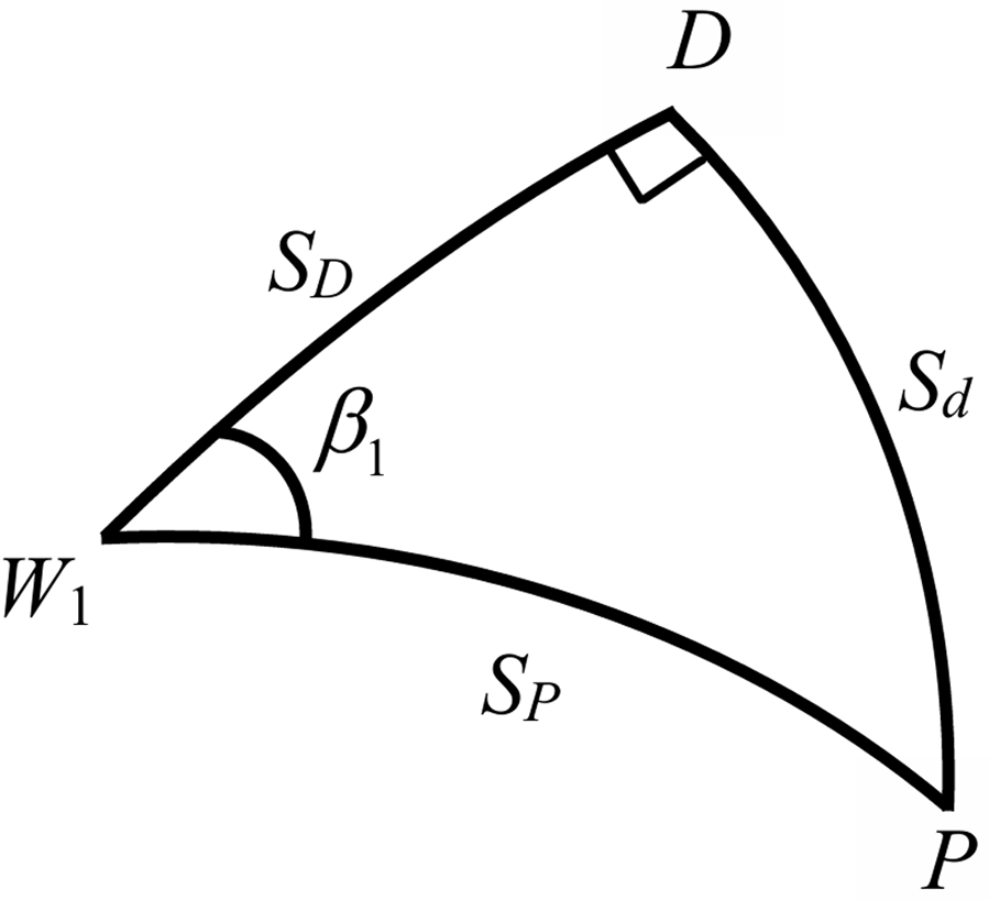
. This forms a spherical right triangle
 $PD{W_1}$
, as shown in Figure 4. Therefore,
 ${\beta _1} = {\beta _P} - {C_1}$
 $\sin {S_d} = \sin {\beta _1}\sin {S_P}$
 $\sin {S_D} = \tan {S_d}\tan (90^\circ - {\beta _1})$
where
 ${S_d}$
is the perpendicular distance from
 $P$
to
 $D$
;
 ${S_D}$
denotes the distance from
 ${W_1}$
to
 $D$
;
 ${\beta _1}$
represents the angular separation between the two great-circle arcs
 ${W_1}{W_2}$
and
 ${W_1}P$
.
Schematic diagram of the spherical triangle.

The coordinates of the point
 $D$
and the great-circle course can be calculated using the following formulae:
 $\cos {\varphi _D} = \sin {\varphi _1}\sin {S_D} + \cos {\varphi _1}\cos {S_D}\cos {C_1}$
 $\cos D{\lambda _D} = {{\cos {S_D} - \sin {\varphi _1}\sin {\varphi _D}} \over {\cos {\varphi _1}\cos {\varphi _D}}}$
 ${\lambda _D} = {\lambda _1} + D{\lambda _D}$
 $\tan {C_D} = {{\sin {\varphi _2}\cos {\varphi _D} - \cos {\varphi _2}\sin {\varphi _D}\cos \left| {{\lambda _2} - {\lambda _D}} \right|} \over {\cos {\varphi _D}\sin \left| {{\lambda _2} - {\lambda _D}} \right|}}$
where
 $D{\lambda _D}$
is the difference in longitude from the starting point to point
 $D$
;
 ${\varphi _D}$
denotes the latitude of point
 $D$
;
 ${\lambda _D}$
represents the longitude of point
 $D$
; and
 ${C_D}$
is the great-circle course at point
 $D$
.
-
(3) Calculate the target point coordinates and the desired course. Let the tracking target be located at a point
$T({\varphi _T},{\lambda _T})$
, which is a great-circle distance
${S_T}$
ahead of the perpendicular foot
$D({\varphi _D},{\lambda _D})$
. The value of
${S_T}$
is determined through multiple experiments,


 $\cos {\varphi _T} = \sin {\varphi _D}\sin {S_T} + \cos {\varphi _D}\cos {S_T}\cos {C_D}$
 $\cos D{\lambda _T} = {{\cos {S_T} - \sin {\varphi _D}\sin {\varphi _T}} \over {\cos {\varphi _D}\cos {\varphi _T}}}$
 ${\lambda _T} = {\lambda _D} + D{\lambda _T}$
 $\tan {C_T} = {{\sin {\varphi _2}\cos {\varphi _T} - \cos {\varphi _2}\sin {\varphi _T}\cos \left| {{\lambda _2} - {\lambda _T}} \right|} \over {\cos {\varphi _T}\sin \left| {{\lambda _2} - {\lambda _T}} \right|}}$
where
 $D{\lambda _T}$
is the difference in longitude from point
 $D$
to point
 $T$
;
 ${\varphi _T}$
denotes the latitude of point
 $T$
;
 ${\lambda _T}$
is the longitude of point
 $T$
;
 ${C_T}$
represents the great-circle course at point
 $T$
. As well as
 ${C_T}$
represents the desired heading in the improved LOS algorithm.
Then, derived from the current ship placement, calculate the target point location and the great-circle course
 ${C_T}$
, which is the desired course. There will be a difference between
 ${C_T}$
and the ship’s starting heading
 $\psi $
, which is the course that needs to be adjusted. By progressively minimising the discrepancy between the intended course and the actual course of the ship, the vessel will follow the great-circle route.
3.3. Design of control system
The closed-loop gain shaping scheme, as a simplified engineering implementation of robust control, is characterised by its basic solution procedure and ease of engineering application. The controller designed with this method has strong robustness. In this paper, a third-order closed-loop gain-shaping method is used to layout the controller
 $K$
. Let the bandwidth frequency of the closed-loop system be
 $1/{T_1}$
, then the complementary sensitivity function
 $T$
of the ship’s course-conserving control structure, which is also the closed-loop transmit capacity of the mechanism, is
 $T = {1 \over {{{({T_1}s + 1)}^3}}} = {{{G_{\psi \delta }}(s)K} \over {1 + {G_{\psi \delta }}(s)K}}$
Then, the ultimate robust controller can be expressed as
 $K = {{{T_0}{\rm{s + }}1} \over {{K_0}{T_1}({T_1}^2{{\rm{s}}^2} + 3{T_1}{\rm{s}} + 3)}} = \left({{{T_0}{\rm{s}}} \over {{K_0}{T_1}}} + {1 \over {{K_0}{T_1}}})({1 \over {{T_1}^2{{\rm{s}}^2} + 3{T_1}{\rm{s}} + 3}}\right)$
From Equation (32), it is evident that the structure of the controller resembles a typical proportional-derivative (PD) controller combined in series with an oscillatory component. This form is concise and very easy to implement, solving the problems of complex parameter tuning and unclear physical meaning associated with conventional PD controllers.
In practical operations, ships have large inertia, which requires a longer adjustment time for control. Under a PD controller, a constant
 $\rho $
is introduced. This allows the system to significantly reduce the adjustment time without compromising stability. Analogous to this method, a positive constant can be added to the proportional part of the PD term in Equation (32). In this paper, based on simulation tests, the constant
 $\rho = 2$
is chosen to get the optimal performance, resulting in the final form of the controller as (Li and Zhang, Reference Li and Zhang2023)
 $K = \left({{{T_0}{\rm{s}}} \over {{K_0}{T_1}}} + {1 \over {{K_0}{T_1}}} + \rho \right)\left({1 \over {{T_1}^2{{\rm{s}}^2} + 3{T_1}{\rm{s}} + 3}}\right)$
3.4. Coordinate transformation
The Mercator map projection is a widely adopted plane projection method for maritime chart creation. It enables the mapping of the Earth’s curved surface onto a flat plane, thereby facilitating the use of nautical charts. A key feature of this projection is its preservation of course linearity; however, it substantially exaggerates areas near the poles, leading to significant distortions in high-latitude regions.
A planar map (usually referring to a map in a Cartesian coordinate system) is typically represented based on a simple Cartesian coordinate system (such as
 $x$
and
 $y$
coordinates).
-
(1) Mercator Projection Coordinates Planar Coordinates Conversion. If the latitude and longitude of a point
$(\varphi, \lambda )$
are known, the following formula can be used to convert it to planar coordinates:

 $x = R\lambda $
 $y = R\ln \left[\tan \left({\pi \over 4} + {\varphi \over 2}\right)\right]$
Here,
 $R$
is the Earth’s radius, typically taken as approximately 6371 km (if different units such as metres and miles are used,
 $R$
also needs to be adjusted accordingly);
 $x$
and
 $y$
correspond to the Cartesian coordinates on the plane;
 $\lambda, \varphi $
are the Mercator projection coordinates for longitude and latitude, respectively.
The longitude and latitude in the above formula need to be in radians. If the longitude and latitude data are in degrees, they first need to be converted to radians:
 ${\lambda _{{\rm{radian}}}} = {\lambda _{{\rm{angle}}}}{\pi \over {180}}$
 ${\varphi _{{\rm{radian}}}} = {\varphi _{{\rm{angle}}}}{\pi \over {180}}$
-
(2) Planar Coordinates to Mercator Projection Coordinates. If you already have the planar coordinates
$(x,y)$
and want to convert them back to the Mercator projection’s latitude and longitude, you can use the inverse formula for conversion:

 $\lambda = {x \over R}$
 $\varphi = 2\arctan ({e^{{y \over R}}}) - {\pi \over 2}$
By converting the ship’s position from planar coordinates to coordinates on a Mercator projection nautical chart, the guidance strategy can better meet the actual navigation requirements, as a result, the practicality and applicability of the control structure are improved.
4. Simulation verification
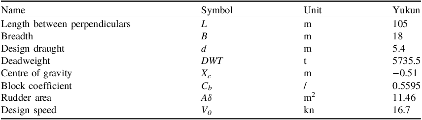
The simulation of the maritime path of the YUKUN from the Bahamas Islands (approximate position: latitude 24°48.0′N, longitude 75°48.0′W) to the Strait of Gibraltar (approximate position: latitude 36°00.0′N, longitude 5°12.6′W) was conducted. The main design parameters of the YUKUN are shown in Table 1. The initial ship’s heading was set at 070° and wind conditions of Beaufort scale 6 were established. To reduce simulation time and accelerate the programme response speed, the radius of the Earth was reduced by a factor of 1000. In the simulations of this study, after multiple rounds of simulation validation,
 ${S_T}$
is set to 200. The simulation tested the performance of three navigation methods, including the great-circle route guidance method proposed in this study, the LOS constant bearing guidance method and the LOS-based approximate great-circle segment guidance method. The simulation outcomes are presented in Figures 5 to 8.
Main design particulars of ‘Yukun’ ship

Table 1 Long description
A table titled 'Main design particulars of Yukun ship' with nine rows and four columns. The columns are labeled 'Name', 'Symbol', 'Unit', and 'Yukun'. The rows list the following data: Row 1: Name, L, m, 105; Row 2: Breadth, B, m, 18; Row 3: Design draught, d, m, 5.4; Row 4: Deadweight, DWT, t, 5735.5; Row 5: Centre of gravity, Xc, m, -0.51; Row 6: Block coefficient, CB, /, 0.5595; Row 7: Rudder area, Aδ, m^2, 11.46; Row 8: Design speed, V0, kn, 16.7.
Track comparison.

Figure 5 Long description
Panel A: A world map showing a great circle route, a rhumb line, and an approximate great circle route between the Bahamas and Gibraltar. The great circle route is marked in red, the rhumb line in pink, and the approximate great circle in green. Key locations include the Bahamas and Gibraltar, highlighted with green markers. Panel B: A zoomed-in view of the North Atlantic region, detailing the same routes and markers as in Panel A. The map uses a grid overlay for precise location reference.
Heading comparison.

Rudder angle comparison.

Tracking error comparison.

The findings in Figure 5 indicate that all three navigation methods designed in this chapter – the great-circle route guidance method, the constant course guidance method based on LOS and the approximate great-circle segmented guidance method based on LOS – can all navigate stably along the planned route under the influence of Beaufort Scale 6 wind conditions.
From Figure 6, it can be observed that with the initial ship heading set to 070°, the heading adjustment behaviours of the three methods are as follows: the great-circle navigation method adopts an initial heading of 061.1°, whereas the constant course navigation method uses an initial heading of 079.5°. During the simulation, the initial heading of the ship is gradually adjusted. The great-circle navigation method began to stably track the reference heading after about approximately 100 s, after which the ship’s heading increased uniformly with changes in position. The constant course navigation method stabilised in tracking the reference heading for approximately 100 s and then maintained a stable heading. In comparison, the approximate great-circle segmented navigation method requires heading adjustments at each segment, resulting in continuous heading changes throughout the simulation. It is important to note that due to the reduction of the Earth’s radius by a factor of 1,000 in the simulation, the heading adjustments for the segmented navigation method occur more frequently. In actual navigation, this frequency of adjustment would be significantly reduced.
As is shown in Figure 7, both the great-circle navigation approach and the constant course navigation method are primarily in the controller adjustment phase within the first 100 s, leading to more pronounced rudder angle variations. After about 100 s, the controller begins to stably track the reference signal and the rudder angle stabilises, with only minor adjustments made in response to high-frequency disturbances from waves. In contrast, the approximate great-circle segmented navigation method requires heading changes at each segment, leading to frequent and larger rudder angle adjustments throughout the entire simulation process.
Figure 8 further illustrates the changes in tracking deviation. In the early stages of the simulation, due to an initial heading difference of approximately 10° between the ship’s initial heading and the reference heading, the ship needs to continuously adjust its heading to track the reference signal, resulting in a relatively large tracking deviation. However, after approximately 100 s of adjustment, the controller can stably follow the reference heading and the tracking error is substantially reduced. Throughout the entire navigation process, the maximum tracking error for the constant course guidance method based on LOS is approximately 25 m, while the maximum tracking error for the approximate great-circle segmented guidance method based on LOS is approximately 40 m. In contrast, the great-circle route guidance and control strategy designed in this section achieves a maximum tracking error of only 6 m over the entire journey, demonstrating a significant advantage.
From Table 2, the value for the great circle remains constant because the course undergoes continuous linear variation. In contrast, the value for the rhumb line is 0 since there is no course change. For the approximate great circle, multiple values are observed due to the presence of course fluctuations. The great circle exhibits the smallest rudder angle variation, indicating the highest level of stability. Finally, although both the great circle and rhumb line exhibit deviations from the route, the variation amplitude of the great circle is smaller than that of the rhumb line in the initial phase. Meanwhile, the approximate great circle shows the largest variation amplitude among the three.
Quantitative analysis after the simulation stabilizes

Table 2 Long description
The table compares three navigation methods: Great circle, Rhumb line, and Approximate great circle. It has four rows and three columns. The columns are labeled Course change rate within 200 s, Maximum value of rudder angle variation (degrees), and Maximum value of route deviation (m). Row 1: Great circle, Course change rate within 200 s, 0.04, Maximum value of rudder angle variation (degrees), 4.6, Maximum value of route deviation (m), 4.1. Row 2: Rhumb line, Course change rate within 200 s, 0, Maximum value of rudder angle variation (degrees), 5.5, Maximum value of route deviation (m), 1.1. Row 3: Approximate great circle, Course change rate within 200 s, 0.08/-0.06, Maximum value of rudder angle variation (degrees), 18.39, Maximum value of route deviation (m), 41.3.
In summary, all three navigation methods are capable of effectively tracking great-circle routes under the same simulation environment. However, there are significant differences among them in terms of the frequency and magnitude of course adjustments, as well as the control of tracking errors. The great-circle navigation method and the loxodrome navigation method demonstrate relatively stable course-keeping control with fewer occurrences of abrupt rudder angle adjustments. In contrast, the segmented great-circle approximation method, which requires frequent course changes, results in larger rudder angle variations, thereby increasing the control complexity and the difficulty of operation. The control algorithm designed in this section has shown a distinct advantage in tracking accuracy, especially in terms of tracking error performance. Compared with the other two methods, the control method proposed in this section can navigate along the great-circle route with the smallest error and with a lower frequency of course adjustments in practical applications. This avoids frequent large-magnitude rudder angle adjustments, thereby enhancing the stability and reliability of navigation. These superior performance characteristics endow the control algorithm designed in this section with strong application potential in the field of navigation control, particularly for navigation tasks that require high-precision track keeping.
5. Conclusions
The guidance and control strategy for great-circle routes based on Mercator projection charts proposed in this paper successfully addresses the challenges of long voyages, the effects of Earth’s curvature and the limitations of traditional navigation methods faced by ships during ocean navigation. By designing the guidance strategy for great-circle routes through the analysis of spherical triangles and combining it with a closed-loop gain-scheduling algorithm to achieve precise ship track-keeping control, this strategy overcomes the issue of traditional methods’ inability to make real-time course adjustments during navigation, ensuring stable ship travel along the great-circle arc. Moreover, by transforming the ship’s position from a planar map to a Mercator projection chart, the guidance strategy better meets the practical needs of maritime engineering, enhancing the applicability and practicality of the control system. This method not only improves the stability of ship travel along great-circle routes, but also effectively reduces navigation time and fuel consumption, thereby enhancing navigation efficiency and economy.
6. Discussions
In the current simulation, only the wind force model has been incorporated to simulate the wind-induced effects on the ship. However, in actual marine environments, the impact of ocean waves is equally crucial for the ship. Future research can integrate a comprehensive wind-wave disturbance model to fully simulate the real operating conditions of ships at sea, thereby making the conclusions more consistent with practical scenarios. Furthermore, When the radius is reduced by 1,000 times, the Earth model becomes smaller and the curvature of the spherical surface increases significantly. This means that the originally long-distance route will appear more curved on the scaled-down model, with a more pronounced visual deviation from a straight line. Meanwhile, when the radius is reduced by 1,000 times, all distances calculated via spherical trigonometry will also be reduced by 1,000 times. Consequently, the relative impact of small errors in angle calculations will be amplified, which may lead to a decline in navigation accuracy. In future research, the real radius of the Earth can be adopted for calculations, which is more consistent with practical application scenarios.
However, since the actual Earth’s surface is not a perfect sphere, the guidance algorithm based on a spherical model suggested in this study may face certain limitations in terms of accuracy during actual navigation. Future research can further optimise the guidance strategy by incorporating the Earth’s ellipsoidal shape model and real-time data on environmental changes during navigation to improve the system’s high-precision navigation capabilities. Meanwhile, the great circle route navigation method proposed in this paper is only applicable to scenarios within the same longitude zone (both the departure point and the destination are in the eastern longitude region or the western longitude region). Future research can extend to navigation scenarios crossing the 180° meridian and other broader application fields to achieve more comprehensive coverage of great-circle routes. Finally, due to the lack of an actual ship to verify the reliability of the proposed method, this paper only validates its feasibility through simulations. In future research, real-ship sea trials can be conducted to further confirm the feasibility of this method.
Acknowledgments
The authors would like to thank anonymous reviewers for their valuable comments to improve the quality of this article.
Funding statement
This work is partially supported by the National Natural Science Foundation of China [Grant No. 51679024], the Joint Program of Science and Technology Plan of Liaoning Province (Key Research and Development Program Project) [Grant No. 2025JH2/101800233], the Dalian Innovation Team Support Plan in the Key Research Field [Grant No. 2020RT08], the Basic Scientific Research Project of Liaoning Education Department [Grant No. LJ212410151025], and the 2023 DMU navigation college first-class interdisciplinary research project [Grant No. 2023JXA06].