2 Weakly compressible theory

Consider gas bubble dynamics in an irrotational and compressible liquid flow. A Cartesian coordinate system is chosen, with the origin at the centre of the bubble at inception, and the $z$ -axis in the direction opposite to gravity.

The reference length is chose as the maximum bubble radius, $R_{max}$ , that a bubble would expand to in an inviscid liquid and without surface tension effects. The density ${\it\rho}_{\infty }$ in the undisturbed liquid is chosen as the reference density. The reference pressure is ${\rm\Delta}p=p_{\infty }-p_{v}$ , where $p_{\infty }$ is the pressure in the undisturbed liquid and $p_{v}$ is the partial pressure of vapour inside the bubble. The vapour pressure $p_{v}$ is approximately a function of the temperature of the bubble wall only, if the time scales of condensation and evaporation are small compared to the period of the bubble oscillation. It is usually small ( $p_{v}\sim 2~\text{kPa}$ at $20\,^{\circ }\text{C}$ ) compared to the hydrostatic pressure and is often negligible (Brennen Reference Brennen1995). The reference velocity is thus obtained as $U=\sqrt{{\rm\Delta}p/{\it\rho}_{\infty }}$ . We introduce dimensionless quantities denoted by subscripts ‘ $\ast$ ’ as follows:

where $\boldsymbol{r}=(x,y,z)$ , $t$ is the time, ${\it\varphi}$ is the velocity potential of the liquid flow and $p$ is the pressure. The speed of sound $c$ is normalized by its value in the undisturbed liquid $c_{\infty }$ .

The highest speed of the liquid flow induced by bubble dynamics is usually associated with the velocity of the bubble jet, which is often lower than $200~\text{m}~\text{s}^{-1}$ at normal ambient pressure, as observed in experiments (Benjamin & Ellis Reference Benjamin and Ellis1966; Lauterborn & Bolle Reference Lauterborn and Bolle1975; Shima et al. Reference Shima, Takayama, Tomita and Miura1981; Tomita & Shima Reference Tomita and Shima1986; Vogel, Lauterborn & Timm Reference Vogel, Lauterborn and Timm1989; Vogel et al. Reference Vogel, Schweiger, Frieser, Asiyo and Birngruber1990; Lauterborn & Ohl Reference Lauterborn and Ohl1997; Philipp & Lauterborn Reference Philipp and Lauterborn1998; Lindau & Lauterborn Reference Lindau and Lauterborn2003; Brujan & Matsumoto Reference Brujan and Matsumoto2012; Yang, Wang & Tan Reference Yang, Wang and Tan2013; Zhang et al. Reference Zhang, Cui, Cui and Wang2015). As the speed of sound in water is approximately $1500~\text{m}~\text{s}^{-1}$ , the flow induced by the bubble dynamics is assumed to be associated with a low Mach number, ${\it\varepsilon}$ , defined as follows:

Lauterborn & Vogel (Reference Lauterborn, Vogel and Delale2013) observed that the newly formed laser bubble’s surface expands with an initial velocity of approximately $2450~\text{m}~\text{s}^{-1}$ , which decays rapidly to approximately $250~\text{m}~\text{s}^{-1}$ within 140 ns. The present model is only valid after that. Note that the term ‘bubble inception’ used in the paper refers to the moment during the early stage of expansion when the bubble wall Mach number starts being small.

We divide the fluid domain into two regions: the inner region near the bubble where $(x,y,z)=O(R_{max})$ and the outer region far away from the bubble where $(x,y,z)=O({\it\lambda})$ , where ${\it\lambda}=c_{\infty }R_{max}/U$ is the wavelength of the acoustic waves.

Using the method of matched asymptotic expansions, the outer solution was shown to satisfy the wave equation to second order and was found analytically as follows (Wang Reference Wang2013, Reference Wang2014):

where $\tilde{r}=r/{\it\lambda}={\it\varepsilon}r_{\ast }$ , $r=|\boldsymbol{r}|$ , and $C_{0}$ is a given constant with a value of $1/(4{\rm\pi})$ and $1/(2{\rm\pi})$ for a bubble in an unbounded liquid and near a rigid boundary, respectively. The quantity $m_{0}(t_{\ast })$ is obtained from matching the inner and outer expansions using Van Dyke’s matching principle (Van Dyke Reference Van Dyke1975; Wang Reference Wang2013, Reference Wang2014) as follows:

where $\boldsymbol{n}$ is the unit normal vector on the bubble surface and the overdot denotes the derivative with respect to time.

The inner solution to second order satisfies Laplace’s equation and the kinematic and dynamic boundary conditions on the bubble surface $S$ as follows (Wang & Blake Reference Wang and Blake2010):

where ${\it\delta}=\sqrt{{\it\rho}gR_{m}/{\rm\Delta}p}$ is the buoyancy parameter and where $g$ is the gravitational acceleration. The liquid pressure $p_{L}$ on the bubble surface is given by, where $p_{B^{\ast }}$ is the pressure of the bubble contents, $p_{g0^{\ast }}=p_{g0}/{\rm\Delta}p$ is the initial partial pressure of the non-condensable gases inside the bubble, $V_{0^{\ast }}$ is the initial bubble volume, ${\it\kappa}$ is the polytropic index of the bubble gas, $\boldsymbol{{\rm\nabla}}\boldsymbol{\cdot }\boldsymbol{n}$ provides the surface curvature and ${\it\sigma}_{\ast }={\it\sigma}/(R_{m}{\rm\Delta}p)$ is the surface tension parameter. Here variables with the subscript of ‘ $\ast$ ’ are dimensionless. We assumed in (2.6) that the expansion and contraction of the bubble gases occur adiabatically. We will not consider the thermal effects associated with this phenomenon, which can lead to chemical reactions (Suslick Reference Suslick1990) and sonoluminescence (Hiller, Putterman & Weninger Reference Hiller, Putterman and Weninger1998; Hilgenfeldt et al. Reference Hilgenfeldt, Brenner, Grossman and Lohse1998; Hilgenfeldt, Grossmann & Lohse Reference Hilgenfeldt, Grossmann and Lohse1999). Fuster & Montel (Reference Fuster and Montel2015) showed that that for very fast oscillations, the effective polytropic coefficient of the mixture recovers the adiabatic limit given that neither heat nor mass transfer has time to significantly modify the pressure inside the bubble. The thermal processes typically absorb a relatively small portion of the overall energy (Akhatov et al. Reference Akhatov, Lindau, Topolnikov, Mettin, Vakhitova and Lauterborn2001). Heat and mass transfer across the bubble surface can be included in the model (Szeri et al. Reference Szeri, Storey, Pearson and Blake2003).

We also assume in (2.6) that the pressure field in the bubble interior is uniform since the density of gases is usually three orders of magnitude smaller than that of liquids. Geers & Zhang (Reference Geers and Zhang1994), Geers & Hunter (Reference Geers and Hunter2002), Geers et al. (Reference Geers, Lagumbay and Vasilyev2012) employed the doubly asymptotic approximations for spherical bubble dynamics for both the external liquid and the internal gases. They noticed that while acoustic wave effects in the external liquid are important, such effects in the internal gases are not.

The far-field boundary condition of the inner solution is obtained by matching with the outer solution as follows:

The initial condition on the boundary is given as

where $R_{0^{\ast }}$ and $R_{t0^{\ast }}$ are the initial radius of the bubble and the initial rate of change of the bubble radius, respectively.

Examining the initial and boundary value problem of (2.5), (2.6), one can see that the compressible effects to second order appear only in the far-field condition (2.6c ). As the basic equation is Laplace’s equation, this problem can be modelled using the BIM. The details on the numerical model using the BIM for this problem can be found in Wang et al. (Reference Wang, Yeo, Khoo and Lam1996a ), Curtiss et al. (Reference Curtiss, Leppinen, Wang and Blake2013).

A non-spherical bubble collapse often leads to the formation of a high-speed liquid jet. The jet subsequently impacts on the opposite bubble surface and penetrates through the bubble, and the liquid domain is then transformed from a singly connected to a doubly connected domain. The solution to a potential problem in a doubly connected domain is non-unique. The doubly connected domain can be made singly connected by, for example, using a branch cut as done by Best (Reference Best1993) or a vortex sheet as done by Zhang, Duncan & Chahine (Reference Zhang, Duncan and Chahine1993) and Zhang & Duncan (Reference Zhang and Duncan1994).

Pedley (Reference Pedley1968) and Lundgren & Mansour (Reference Lundgren and Mansour1991) modelled the dynamics of a bubble torus with a vortex ring inside, starting with a circular cross-section. Wang et al. (Reference Wang, Yeo, Khoo and Lam1996b , Reference Wang, Yeo, Khoo and Lam2005) developed a vortex ring model from these earlier ideas to model the topological transition of a singly connected bubble to a subsequent toroidal bubble. In the vortex ring model, a vortex ring is put inside the toroidal bubble after jet impact. The circulation of the vortex ring is equal to the jump of the potential ${\it\varphi}_{\ast }$ across the contact point at the time of jet impact

where ${\it\varphi}_{N^{\ast }}$ and ${\it\varphi}_{S^{\ast }}$ are potentials at the impact point. Here we assume jet impact occurs at a single point. The potential ${\it\varphi}_{\ast }$ is then decomposed as follows:

where ${\it\varphi}_{vr}$ is the potential of the vortex ring which can be obtained from the Biot–Savart law. With the potential jump being accounted for by the vortex ring using (2.8), the remnant potential ${\it\phi}$ is continuous in the flow field and can be simulated using the BIM model (Wang et al. Reference Wang, Yeo, Khoo and Lam2005).

Zhang et al. (Reference Zhang, Duncan and Chahine1993) considered the loss of the mechanical energy due to jet impact and obtained a formula for the energy loss, which exists when the impact occurs over a finite area. Rogers et al. (Reference Rogers, Szymczawk, Bergera and Soloman1990) and Szymczawk et al. (Reference Szymczawk, Rogers, Soloman and Bergera1993) also noted an energy loss during impact and presented a similar formula. Jet impact often happens on a small area, since the curvature radius of the jet front is usually smaller than the curvature radius of the opposite bubble wall at the location of impact. Important energy conversions following jet impact and jet penetration through the bubble, which may result in bubble mass loss, formation of numerous satellites microbubbles and bubble fission and formation of bubble clouds. Although jet impact may be more complex in reality, we assume in this paper that jet impact occurs at a point, an idealized model, and do not calculate the loss and conversion of energy due to jet impact.

3 Local energy of a bubble system in a compressible liquid

This paper is concerned only with the mechanical energy of a bubble system not considering for heat transfer, evaporation or condensation etc. The total mechanical energy $E_{T}$ of a bubble system consists of the local energy $E_{L}$ within the inner region and the acoustic radiation energy $E_{A}$ radiated outside of the inner region, i.e.

It is natural to separate the mechanical energy of a bubble system into the local energy and acoustic radiation energy, since different length/time scales of decay are associated with the incompressible fluid motion and the acoustic radiation associated with the bubble dynamics.

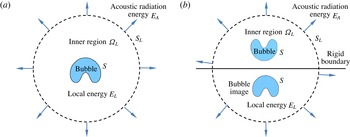
For a bubble system in a compressible liquid, the inner region ${\it\Omega}_{L}$ is bounded by the bubble surface $S$ and a large sphere $S_{L}$ , with its centre at the centre of the initial bubble surface and a radius $R_{L}$ , as shown in figure 1(a). $R_{L}$ is much larger than the maximum bubble radius $R_{max}$ but much smaller than the wavelength ${\it\lambda}$ : $R_{max}\ll R_{L}\ll {\it\lambda}$ . The local mechanical energy $E_{L}$ of a bubble system consists of the local potential energy $E_{LP}$ and the local kinetic energy $E_{LK}$ within $S_{L}$ .

Figure 1.

(a) Illustration of the inner region ${\it\Omega}_{L}$ of the flow field for a bubble in an infinite domain bounded by the bubble surface $S$ and a large sphere $S_{L}$ , with its centre at the centre of the initial bubble surface and with a radius $R_{L}$ satisfying $R_{max}\ll R_{L}\ll {\it\lambda}$ , where $R_{max}$ and ${\it\lambda}$ are the maximum equivalent bubble radius and the wavelength of acoustic waves, respectively. The total mechanical energy $E_{T}$ of a bubble system consists of the local energy $E_{L}$ within the inner region and the acoustic radiation energy $E_{A}$ radiated outside of the inner region. (b) Illustration of the inner region ${\it\Omega}_{L}$ of the flow field for a bubble near a rigid flat boundary, using the method of image.

For a bubble near a flat rigid boundary, it is equivalent to the interaction of the bubble and its image to the boundary, as illustrated in figure 1(b). The inner region is then bounded by the bubble surface $S$ , its image and a large sphere $S_{L}$ , with its centre at the centre of the two bubble surfaces at the inception and the radius $R_{L}$ .

4 A spherical bubble system

Dynamics of a spherical bubble in a compressible liquid can be described approximately by the Keller–Miksis equation,

where

where $p_{a^{\ast }}(t_{\ast })$ is the acoustic pressure at the location of the centre of the initial bubble and $Re={\it\rho}_{\infty }UR_{max}/{\it\mu}$ is the Reynolds number, with ${\it\mu}$ being viscosity. Geers & Zhang (Reference Geers and Zhang1994), Geers & Hunter (Reference Geers and Hunter2002), Geers et al. (Reference Geers, Lagumbay and Vasilyev2012) compared the Keller–Miksis equation with the numerical solution of the Euler equation for spherical bubbles for large parameter ranges. They noticed that weakly compressible theory provides very accurate results.

Figure 2.

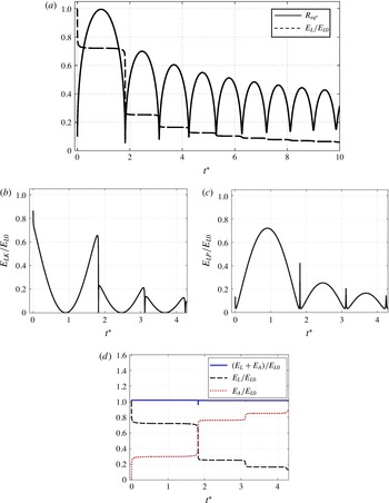
Time histories for the spherical bubble generated by a detonation equivalent to 1.32 g of TNT at 1.5 m below the water surface: (a) the radius $R_{\ast }$ and local energy $E_{L}$ of the bubble system, non-dimensionalized by the initial local energy $E_{L0}$ , (b) the local kinetic energy $E_{LK}$ , (c) the local potential energy $E_{LP}$ and (d) the energy balance. The other parameters used for calculation are ${\it\kappa}=1.667$ , ${\it\varepsilon}=0.0072$ , $p_{v^{\ast }}=0$ , ${\it\sigma}_{\ast }=0$ , $R_{0^{\ast }}=0.1$ , $R_{t0^{\ast }}=28.1$ and $p_{0^{\ast }}=122$ . The energy is non-dimensionalized by the initial local energy $E_{L0}$ .

The Keller–Miksis equation is integrated using the fourth-order Runge–Kutta method to obtain $R(t)$ , ${\dot{R}}(t)$ and $\ddot{R}(t)$ and $V(t)$ , $\dot{V}(t)$ and $\ddot{V}(t)$ . With that the energy flux $N_{flux}$ and the radiated energy $E_{A}$ to the far field can be calculated using (3.11). The calculations were performed for relative and absolute tolerances being 10 $^{-4}$ , since the results are remained almost the same for smaller relative and absolute tolerances.

The first case considered is for an underwater explosion bubble with a maximum equivalent radius $R_{max}=171.2$  mm initiated at 1.5 m below the water surface, generated by a detonation equivalent to 1.32 g of TNT (Hung & Hwangfu Reference Hung and Hwangfu2010). The computational parameters are chosen as ${\it\kappa}=$ 1.667, ${\it\varepsilon}=0.0072$ , $R_{0^{\ast }}=0.1$ , $R_{t0^{\ast }}=28.1$ and $p_{0^{\ast }}=122$ (Wang Reference Wang2013). Figure 2(a) shows the history of the local energy of the bubble system versus the history of the bubble radius. The bubble undergoes several cycles of oscillation, each time with reduced amplitude owing to the loss of the local energy. The local energy remains nearly constant during most of the oscillation, except for very short periods in the vicinity of each minimum volume, when it decreases rapidly. It decreases by approximately 28 % during a very short period at the start of the first expansion phase but remains nearly constant during most of the first cycle of oscillation. The local energy subsequently reduces by 47 %, 8.5 %, 3.9 %, 2.3 % and 1.4 % at the ends of the first to fifth collapse phases, respectively, when a pressure impulse is generated and propagates rapidly through the liquid. It remains as constant at 72 %, 25 %, 16.5 %, 12.6 %, 10.3 % and 8.9 % of the initial energy during most of the first to sixth cycles of the oscillation. The energy loss due to the acoustic radiation at the minimum volumes of the bubble reduces with oscillation cycles.

The time histories of the local kinetic energy and potential energy of the bubble system are shown in figures 2(b) and 2(c), respectively. The local potential energy oscillates in phase with the bubble volume, whereas the local kinetic energy oscillates out of phase with the bubble volume. Their amplitudes decrease significantly from the first to the second cycle and from the second to the third cycle. The spikes at the minimum bubble volumes in figure 2(c) are due to the contribution from the potential energy of the bubble gases, which achieves maximum values at these moments.

Figure 2(d) shows the histories of the acoustic radiation energy $E_{A}$ , the local energy $E_{L}$ and the total energy $E_{T}$ . The radiation energy $E_{A}$ increases for a very short period during each minimum volume of the bubble. The total energy $E_{T}$ remains approximately constant during all the time considered, which suggests that the main energy loss is due to acoustic radiation and viscous effects are negligible for this case.

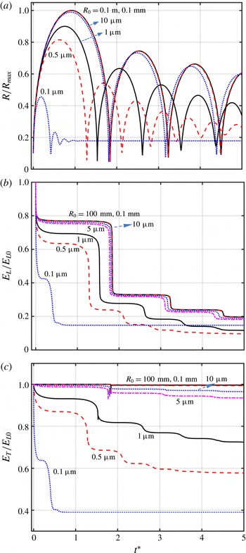
Note $R_{max}$ is the maximum bubble radius that a bubble would expand to in an inviscid liquid and without surface tension effects. The difference between unity and the maximum value of $R/R_{max}$ thus reflects the effects of viscosity and surface tension. Figure 3(a) shows the time history of the bubble radius $R/R_{max}$ for transient bubbles at various initial radii $R_{0}$ over a large range from $0.1~{\rm\mu}\text{m}$ to 100 mm. The remaining parameters are ${\it\rho}_{\infty }=1000~\text{kg}~\text{m}^{-3}$ , ${\it\mu}=0.001~\text{Pa}~\text{s}$ , $c_{\infty }=1500~\text{m}~\text{s}^{-1}$ , $p_{\infty }=100~\text{kPa}$ , $p_{v}=0$ , ${\it\sigma}=0.07~\text{N}~\text{m}^{-1}$ , $R_{0^{\ast }}=0.1$ , $R_{t0^{\ast }}=26.7$ , $p_{g0^{\ast }}=100$ and ${\it\kappa}=1.4$ .

Figure 3.

Time histories of (a) the dimensionless bubble radius $R/R_{max}$ , (b) local energy of the bubble system $E_{L}/E_{L0}$ and (c) total energy $E_{T}/E_{L0}$ , for transient bubbles with initial radius $R_{0}$ ranging from $0.1~{\rm\mu}\text{m}$ to 100 mm. The other parameters are ${\it\rho}_{\infty }=1000~\text{kg}~\text{m}^{-3}$ , ${\it\mu}=0.001~\text{Pa}~\text{s}$ , $c_{\infty }=1500~\text{m}~\text{s}^{-1}$ , $p_{\infty }=100~\text{kPa}$ , $p_{v}=0$ , ${\it\sigma}=0.07~\text{N}~\text{m}^{-1}$ , $R_{0^{\ast }}=0.1$ , $R_{t0^{\ast }}=26.7$ , $p_{g0^{\ast }}=100$ and ${\it\kappa}=1.4$ .

As the initial radius $R_{0}$ decreases, the damping of the bubble oscillation increases. In the range of $R_{0}$ from 0.1 to 100 mm, the time history of $R/R_{max}$ does not change with $R_{0}$ , where both the viscous effects and surface tension effects are negligible. At $R_{0}=10~{\rm\mu}\text{m}$ , the bubble oscillates only slightly differently from the above results, where viscous and surface tension effects are small. As $R_{0}$ is decreased to $1~{\rm\mu}\text{m}$ or smaller, the bubble undergoes obviously more severely damped oscillations.

As shown in figure 3(b), the local energy $E_{L}$ follows a step function falling significantly at the minimum bubble volumes and remaining approximately constant during the remaining time. The energy loss at the minimum bubble volumes decreases with oscillation cycles. In the range of $R_{0}=10~{\rm\mu}\text{m}$ to 100 mm, the history of $E_{L}$ does not change significantly with $R_{0}$ . The local energy reduces faster for a smaller bubble. At $R_{0}=0.5~{\rm\mu}\text{m}$ , the local energy first falls rapidly due to acoustic radiation and then reduces due to viscous effects. This is repeated during the second cycle. More than two-thirds of the local energy is lost for the first cycle of oscillation due to the combined effects of acoustic radiation and viscosity.

Figure 3(c) shows the time history of the total energy $E_{T}$ . In the range of $R_{0}=0.1$ –100 mm, the total energy remains almost constant, with viscous effects being negligible. It only reduces about 0.4 % at the end of the first collapse phase, which should be due to the approximation of the Keller–Miksis equation. Note that the Keller–Miksis equation is based on a weakly compressible theory to second order.

For $R_{0}=10$ , $5~{\rm\mu}\text{m}$ , the total energy $E_{T}$ remains at approximately 97 % and 93.5 % (figure 3 c), respectively, in the fifth oscillation, and therefore the corresponding energy loss due to viscous effects are 3 % and 6.5 %, respectively. At the same time, the local energy remains 19 % and 18 % of the initial value (figure 3 b), respectively, and the energy loss due to compressible effects are thus 78 % and 75.5 %, respectively. This suggests that the loss of the local energy is mainly due to acoustic radiation and viscous effects are negligible when $R_{0}$ is equal to $5~{\rm\mu}\text{m}$ or larger.

Both compressible effects and viscous effects are essential for microbubble dynamics. For $R_{0}=1~{\rm\mu}\text{m}$ , the energy loss due to viscous effects is 18 % and 28 % after the first and fourth cycles of oscillation, respectively, and the corresponding energy loss due to acoustic radiation is 54 % and 60 %, respectively. The local energy is lost faster for a smaller bubble. For $R_{0}=0.5~{\rm\mu}\text{m}$ the loss of the local energy after the first oscillation is approximately 76 %, of which 44 % is due to compressible effects and 32 % due to viscous effects. The energy loss after the first four cycles of oscillation is approximately 90 %, of which 48 % is due to compressible effects and 42 % due to viscous effects. For $R_{0}=0.1~{\rm\mu}\text{m}$ the energy of the bubble system is lost mostly during the first oscillation. The loss of the local energy during the early expansion is approximately 58 %, of which 36 % is due to compressible effects and 22 % due to viscous effects. The energy loss after the first cycle of oscillation is approximately 85 %, of which 24 % is due to compressible effects and 61 % due to viscous effects.

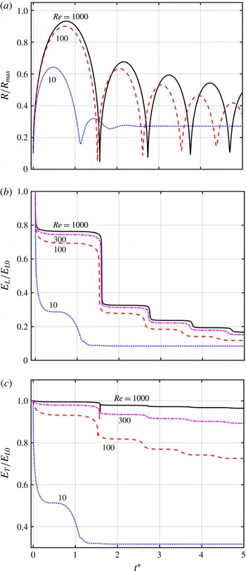
Figure 4 shows the time histories of the dimensionless bubble radius $R_{\ast }$ and local energy $E_{L}/E_{L0}$ , for transient bubbles for ${\it\sigma}_{\ast }=0.07$ and $Re=10$ , 100, 300 and 1000, respectively. The other parameters used are ${\it\varepsilon}=0.00667$ , $p_{v^{\ast }}=0$ , $R_{0^{\ast }}=0.1$ , $R_{t0^{\ast }}=26.7$ , $p_{g0^{\ast }}=100$ and ${\it\kappa}=1.4$ . With the decrease of the Re number, both the oscillation period and maximum bubble radius decrease, whereas the minimum radius increases. For $Re=1000$ , the total energy loss is 84 % after the first four cycles of oscillation, of which 80 % is due to compressible effects and 4 % due to viscous effects. For $Re=300$ , the total energy loss is 72 % after the first oscillation, of which 66 % is due to compressible effects and 6 % due to viscous effects. The total energy loss is 85 % after the first four cycles of oscillation, of which 74 % is due to compressible effects and 11 % due to viscous effects. Compressible effects are thus dominant for $Re=300$ or larger.

Figure 4.

Time histrories of (a) the dimensionless bubble radius $R/R_{max}$ , (b) local energy $E_{L}/E_{L0}$ and (c) the total energy $E_{T}/\max (E_{T})$ , for transient bubbles for ${\it\sigma}_{\ast }=0.07$ and $Re=10$ , 100, 300, 1000, respectively. The other parameters are ${\it\varepsilon}=0.00667$ , $p_{v^{\ast }}=0$ , $R_{0^{\ast }}=0.1$ , $R_{t0^{\ast }}=26.7$ , $p_{g0^{\ast }}=100$ and ${\it\kappa}=1.4$ .

Both compressible effects and viscous effects are essential for $Re=100$ or smaller. For $Re=100$ , the total energy loss is 89 % after the first four cycles of oscillation, of which 61 % is due to compressible effects and 28 % due to viscous effects. For $Re=10$ , the total energy loss is 92 % after the first four cycles of oscillation, of which 34 % is due to compressible effects and 68 % due to viscous effects.

Note here that the Reynolds number $Re$ is defined in terms of the maximum bubble radius $R_{max}$ . The Reynolds number is also often defined in terms of the initial bubble radius, $Re_{0}={\it\rho}UR_{0}/{\it\mu}$ . As $R_{0}=0.1R_{max}$ in the cases, $Re_{0}=0.1Re$ .

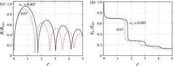
Figure 5 shows the effects of surface tension. The oscillation period and maximum bubble radius decrease with the dimensionless surface tension ${\it\sigma}_{\ast }$ , but the loss of the local energy does not change significantly with ${\it\sigma}_{\ast }$ .

Figure 5.

Time histrories of (a) the dimensionless bubble radius $R/R_{max}$ , and (b) local energy $E_{L}/E_{L0}$ , for transient bubbles for $Re=100$ and ${\it\sigma}_{\ast }=0.007$ , 0.07 respectively. The other parameters are the same as figure 4.

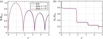
Figure 6 shows the comparison between the Keller–Miksis equation (KM) and the compressible BIM model, for the time histories of the dimensionless bubble radius $R_{\ast }$ and the local energy $E_{L}/E_{L0}$ , for a transient bubble for $R_{0}=100~{\rm\mu}\text{m}$ . The BIM results are calculated for the number of nodes $n=41$ , 51, respectively, showing convergence of the numerical model in terms of the mesh size. The BIM results agree very well with that of the Keller–Miksis equation. This is as expected, since both the Keller–Miksis equation and the compressible BIM model are based on the weakly compressible theory to second order in terms of the Mach number ${\it\varepsilon}$ . Lezzi & Prosperetti (Reference Lezzi and Prosperetti1987) compared the third-order solution with the second-order solution. They noticed that the second-order theory describes the main compressible effects when the Mach number is small, and the third-order solution is a minor correction.

Figure 6.

Comparison between the KM equation and BIM modelling for the number of nodes $n=41$ , 51, respectively, for the time histrories of (a) the dimensionless bubble radius $R/R_{max}$ , and (b) local energy $E_{L}/E_{L0}$ , for a transient bubble for $R_{0}=100~{\rm\mu}\text{m}$ . The other parameters are the same as figure 3.

5 A gas bubble under buoyancy

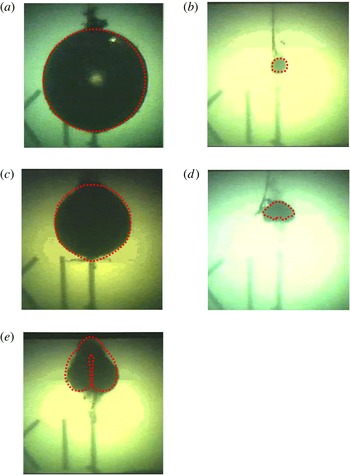
We now consider a non-spherical bubble generated by an underwater explosion of $R_{m}=171~\text{mm}$ and depth $h=1.5~\text{m}$ from the water surface. The bubble shapes calculated for this case using the recently developed compressible BIM model (Wang Reference Wang2013) agree well with experiments (Hung & Hwangfu Reference Hung and Hwangfu2010) for both the first and second cycles of oscillation (see figure 7). The bubble expands spherically reaching the first maximum volume (a), and then collapses spherically. However the lower part of the bubble surface is flattened due to buoyancy at the end of collapse (b), whereupon an upward jet forms, impacts the opposite bubble surface and subsequently penetrates the bubble. The bubble re-expands to a spherical shape at its second maximum volume (c) and then recollapses with a jet forming at the end of recollapse (d). It further rebounds with a sharp jet (e).

Figure 7.

Comparison of the compressible BIM model computation (dotted line) with the experimental images (Hung & Hwangfu Reference Hung and Hwangfu2010) for an underwater explosion bubble of $R_{m}=171~\text{cm}$ and depth $h=1.5~\text{m}$ below the water surface, at times $t=15$ , 27, 36, 48, 51 ms. The image width is 500 mm. The other parameters are ${\it\kappa}=1.667$ , $R_{0}/R_{m}=0.1$ , $R_{t0}=303~\text{m}~\text{s}^{-1}$ , $p_{\infty }=116~\text{kPa}$ and $p_{0}=14.2~\text{MPa}$ .

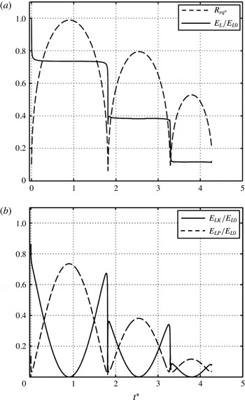
Figure 8(a) shows the time history of the local energy $E_{L}$ of the bubble system versus the equivalent bubble radius $R_{eq^{\ast }}=((3/4{\rm\pi})V_{\ast })^{1/3}$ . A substantial part, 26.5 %, of the local energy is lost during a very short period at the inception of the bubble, when a steep pressure wave is emitted with high pressure amplitude. It remains almost constant at 73.5 % of the initial energy for most of the time during the first cycle but decreases rapidly and significantly at the end of collapse, with the emission of another steep pressure wave. About 35 % of the initial energy is lost this time with only approximately 38.5 % of the initial energy left during the second cycle. As a result, the dimensionless maximum radius reduces from 1.0 during the first cycle to 0.79 during the second cycle. Approximately 27 % of the initial energy is lost around the end of recollapse with only 11.5 % of the initial energy left during the third cycle of oscillation. The dimensionless maximum radius reduces further to 0.53 during the third cycle. The local energy of the bubble system is conserved during most of the time, except for very short periods around the minimum volumes of the bubble.

Figure 8.

Time histories of the bubble system for the case shown in figure 7: (a) the equivalent bubble radius $R_{eq^{\ast }}$ and the local energy $E_{L}$ of the bubble system and (b) the local kinetic energy $E_{LK}$ and potential energy $E_{LP}$ . The energy is non-dimensionalized by the initial local energy $E_{L_{0}}$ .

Figure 8(b) shows that the local potential energy $E_{LP}$ of the bubble system oscillates in phase with the bubble volume while the local kinetic energy $E_{LK}$ oscillates out of phase with the bubble volume. Both of their magnitudes reduce significantly from the first to the second cycles of oscillation and from the second to the third cycles.

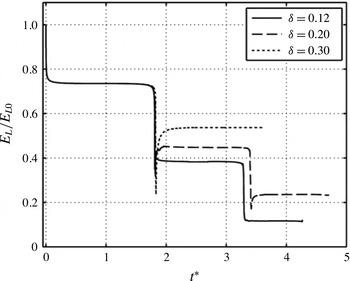
Figure 9 shows that the local energy appears as a step function of time for underwater explosion bubbles for various buoyancy parameters ${\it\delta}=0.12$ , 0.2 and 0.3, corresponding to $R_{m}=171$ , 476 and 1000 mm, respectively. With the initial energy deposited from the explosion, the bubble expands rapidly at inception with the emission of a steep pressure wave; the local energies then fall by approximately 27 % for all three bubbles, when they are small and the buoyancy effects are negligible. The local energy is conserved while the bubbles oscillate but falls rapidly at the end of collapse, when another steep pressure wave is emitted. A larger bubble is associated with stronger buoyancy effects and a stronger liquid jet formed at the end of collapse (Wang Reference Wang2013), and thus its collapse is weaker with less energy loss. Consequently, the energy of the bubble system remains at approximately 39 %, 45 % and 54 % of the initial energy during the second cycle of oscillation for $R_{m}=171$ , 476 and 1000 mm, respectively.

Figure 9.

Time histories of the local energy $E_{L}$ of the bubble system for various buoyancy parameters ${\it\delta}=0.12$ , 0.2 and 0.3 with the remaining parameters being the same figure 7.

This model does not simulate the propagation of pressure waves, but it models the rapid and significant losses of the local energy at the inception of a bubble and the end of collapse. This rapid and significant energy loss should be associated with a steep pressure wave in a narrow region travelling through water. After it propagates radially for a while its amplitude will drop, because the surface wave front is approximately spherical with its area increasing with time.

One of the damage mechanisms of underwater explosions is associated with the steep pressure wave emitted at the inception of the underwater explosion bubble (Wardlaw & Luton Reference Wardlaw and Luton2000; Wardlawet al. Reference Wardlaw, Luton, Renzi, Kiddy and McKeown2003a ,Reference Wardlaw, Luton, Renzi and Kiddy b ). Another damage mechanism is associated with the high-speed liquid jet formed at the end of collapse (Chahine & Perdue Reference Chahine and Perdue1988; Duncan & Zhang Reference Duncan and Zhang1993; Duncan, Milligan & Zhang Reference Duncan, Milligan and Zhang1996; Blake et al. Reference Blake, Hooton, Robinson and Tong1997; Chahine & Harris Reference Chahine and Harris1998a ,Reference Chahine and Harris b ; Wang Reference Wang1998, Reference Wang2004), which is often directed towards a nearby structure (Chahine & Bovis Reference Chahine and Bovis1980; Klaseboer et al. Reference Klaseboer, Hung, Wang, Wang, Khoo, Boyce, Debono and Charlier2005; Jayaprakash, Chao-Tsung & Chahine Reference Jayaprakash, Chao-Tsung and Chahine2010; Jayaprakash, Singh & Chahine Reference Jayaprakash, Singh and Chahine2011).

6 A cavitation bubble near a rigid wall

This section is concerned with cavitation bubble dynamics near a rigid boundary. The cases considered are for a bubble with $R_{m}=1.45~\text{mm}$ at various standoff distance from the boundary, which correspond to the experimental cases by Philipp & Lauterborn (Reference Philipp and Lauterborn1998). The other computational parameters chosen are ${\it\kappa}=1.4$ , ${\it\varepsilon}=0.013$ , ${\it\sigma}_{\ast }=0.00051$ , $R_{0^{\ast }}=0.1$ , $R_{t0^{\ast }}=31$ and $p_{g0^{\ast }}=127$ . The bubble shapes calculated for these cases, using the compressible BIM model (Wang Reference Wang2014) agree well with the experiment for both the first and second cycles of oscillation.

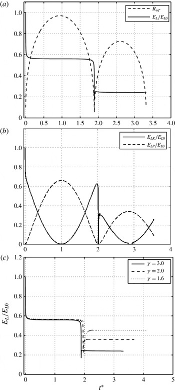
The first case is for a bubble at the dimensionless standoff distance ${\it\gamma}=s/R_{m}=3.0$ from the rigid boundary, where $s$ is the distance of the bubble centre from the rigid boundary at inception. Figure 10(a) shows the time history of the local energy $E_{L}$ of the bubble system versus the time history of the bubble equivalent radius $R_{eq^{\ast }}$ for the first and second cycles of oscillation. The local energy remains constant except for very short periods around the minimum bubble volumes, where it reduces rapidly. The local energy falls by approximately 44 % during its inception and remains at 56 % of the initial energy during most of the first cycle of oscillation. It further reduces by 32 % during the end of collapse and remains at 24 % of the initial energy during the second cycle.

Figure 10(b) shows that the local potential energy $E_{LP}$ of the bubble system oscillates in phase with the bubble volume while the local kinetic energy $E_{LK}$ is out of phase with the bubble volume. Both of their magnitudes reduce significantly from the first to the second cycles of oscillation.

Figure 10.

Time histories of cavitation bubble dynamics near a rigid boundary characterized by ${\it\kappa}=1.4$ , ${\it\varepsilon}=0.013$ , ${\it\sigma}_{\ast }=0.00051$ , $R_{0^{\ast }}=0.1$ , $R_{t0^{\ast }}=31.0$ , $p_{v^{\ast }}=0$ and $p_{g0^{\ast }}=127$ : (a) the equivalent bubble radius $R_{eq^{\ast }}$ and the local energy $E_{L}$ of the bubble system for ${\it\gamma}=3.0$ , (b) the local kinetic energy $E_{LK}$ and potential energy $E_{LP}$ for ${\it\gamma}=3.0$ and (c) the comparison of the local energy at various standoff distances from the rigid boundary for ${\it\gamma}=3.0$ , 2.0 and 1.6 respectively.

Figure 10(c) shows the time histories of the local energy $E_{L}$ of the bubble system at various dimensionless standoff distances from the rigid boundary for ${\it\gamma}=3.0$ , 2.0 and 1.6, respectively. At inception it falls by approximately 44 % at all three standoff distances, when the bubble is small and the effects of the boundary are negligible. The bubble becomes non-spherical during the later stage of collapse, when a high-speed liquid jet forms towards the boundary. When the bubble is nearer to the boundary a stronger jet forms and the collapse becomes relatively weaker (Philipp & Lauterborn Reference Philipp and Lauterborn1998; Wang Reference Wang2014). As a result, the energy loss decreases as the bubble is initiated nearer the boundary, remaining at approximately 24 %, 36 % and 45 % of the initial energy in the second cycle of oscillation for ${\it\gamma}=3.0$ , 2.0 and 1.6, respectively. The local energy loss at the end of collapse decreases rapidly as the standoff distance is decreased. This is true because when the bubble is closer to the boundary, the bubble becomes non-spherical earlier in its oscillation cycle, a larger jet then forms and a larger amount of kinetic energy is associated with the jet (Zhang et al. Reference Zhang, Duncan and Chahine1993; Zhang & Duncan Reference Zhang and Duncan1994; Philipp & Lauterborn Reference Philipp and Lauterborn1998; Wang Reference Wang2014). Consequently, the bubble collapse becomes relatively weaker.

Cavitation damage is generally believed to be due to shock wave emission and bubble jetting formed at the end of collapse (Rayleigh Reference Rayleigh1917; Taylor Reference Taylor1942; Naudé & Ellis Reference Naudé and Ellis1961; Plesset & Chapman Reference Plesset and Chapman1971; Plesset & Prosperetti Reference Plesset and Prosperetti1977; Blake & Gibson Reference Blake and Gibson1987). It was suggested by experimental studies (Tomita & Shima Reference Tomita and Shima1986; Philipp & Lauterborn Reference Philipp and Lauterborn1998; Wang et al. Reference Wang, Manmi and Liu2015) that cavitation erosion is also associated with a bubble ring with high pressure and temperature in direct contact with a rigid boundary formed at the end of recollapse. Chen & Israelachvili (Reference Chen and Israelachvili1991) noticed in experiments that the inception of cavities is intimately connected with simultaneous relaxations of high local strain energies on nearby surfaces. They suggest that in many practical situations, damage is more likely to occur during the formation, rather than the collapse, of cavities. The damage mechanism of Chen & Israelachvili (Reference Chen and Israelachvili1991) is consistent with the result observed here that the local energy of a bubble system at inception is much higher than at the end of collapse.

7 Single bubble sonoluminescence

Single bubble sonoluminescence is an intriguing phenomenon. A gas bubble of only a few micrometres in size is levitated in a liquid by an acoustic standing wave and kept in position at a pressure antinode. As the bubble is compressed periodically by the acoustic wave, it emits light pulses so intense as to be visible to the naked eye with clock-like regularity (Gaitan et al. Reference Gaitan, Crum, Church and Roy1992; Hiller, Putterman & Barber Reference Hiller, Putterman and Barber1992; Gompf et al. Reference Gompf, Günther, Nick, Pecha and Eisenmenger1997; Suslick & Crum Reference Suslick, Crum and Crocker1997; Lohse Reference Lohse2005). This process gives rise to featureless continuum emission in water (from 200 to 800 nm, with increasing intensity into the ultraviolet) (Hiller et al. Reference Hiller, Putterman and Barber1992, Reference Hiller, Putterman and Weninger1998).

The initial pressure of a gas bubble at equilibrium is given as, $p_{g0}=p_{\infty }+2{\it\sigma}/R_{0}$ , which is in balance with the ambient pressure and surface tension. The pressure at the antinode of a standing wave is

where $p_{A}$ and $f$ are the amplitude and frequency of the acoustic wave respectively.

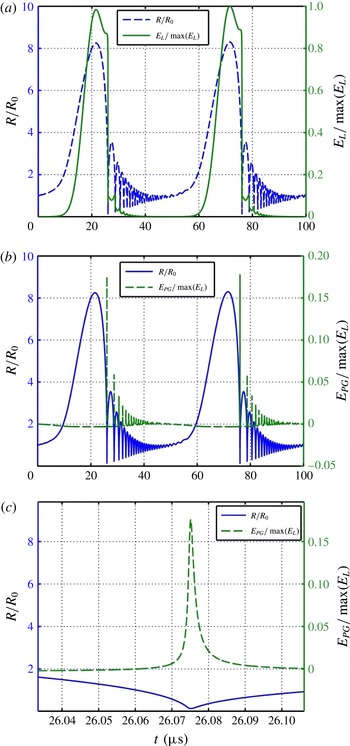
A typical sonoluminescence case is considered using the KM equation, with the parameters chosen as $p_{A}=130~\text{kPa}$ , $f=20~\text{kHz}$ and $R_{0}=5~{\rm\mu}\text{m}$ (Lauterborn & Kurz Reference Lauterborn and Kurz2010). As shown in figure 11(a), the local energy first increases rapidly from nearly zero to its maximum value, within a very short period (about $10~{\rm\mu}\text{s}$ , 20 % of the wave period), by absorbing energy from the acoustic wave. The local energy then decreases more rapidly to nearly zero in approximately $4~{\rm\mu}\text{s}$ (8 % of the wave period) and remains small during the remainder of the cycle, for approximately $35~{\rm\mu}\text{s}$ (70 % of the wave period). The majority of the energy loss (approximately 80 %) happens within $0.1~{\rm\mu}\text{s}$ , which is only 0.2 % of the wave period. As a result, the gas bubble in water is driven into violent oscillation. It expands to more than eight times its equilibrium radius, and then collapses rapidly over a very short time period (about $4~{\rm\mu}\text{s}$ ). The bubble subsequently vibrates with small amplitude at approximately its natural frequency.

Figure 11.

Time histories of a bubble with an initial radius $R_{0}=5~{\rm\mu}\text{m}$ and initial pressure $p_{g0}=1.3~\text{atm}$ (0.3 atm due to surface tension) at the antinode of a standing wave having pressure amplitude $p_{A}=1.3~\text{atm}$ and frequency $f=20~\text{kHz}$ : (a) the local energy $E_{L}$ of the bubble system and the bubble radius $R$ versus time, (b) the potential energy $E_{PG}$ of the bubble gas and the bubble radius $R$ versus time, and (c) an enlarged view of the gas potential energy $E_{PG}$ and radius $R$ near the end of the first collapse.

As shown in figure 11(b) and (c), the potential energy of the bubble gas is small most of the time except for a very short period near the minimum bubble volumes. The gas potential energy is appreciable within a time span of $0.01~{\rm\mu}\text{s}$ (0.02 % of the wave period) at the end of the violent collapse, achieving its maximum of $0.18\max (E_{L})$ , when the bubble is small at $R=0.675~{\rm\mu}\text{m}$ and the energy density of the bubble gas is large at $3.5\times 10^{25}~\text{J}~\text{M}^{-3}$ . In reality, the energy density cannot reach this value due to the evaporation of water, heat transfer and emission of light (Szeri et al. Reference Szeri, Storey, Pearson and Blake2003; Lohse Reference Lohse2005; Zhang & Li Reference Zhang and Li2014). This energy concentration yields very high pressures and temperatures, thus providing the physical internal environment for sonoluminescence and sonochemistry. The local energy describes the energy transfer from the acoustic wave to the bubble system and the subsequent energy concentration due to the bubble collapse.

8 Summary and conclusions

The total mechanical energy $E_{T}$ of a bubble system consists of the local energy $E_{L}$ within the inner asymptotic region and the acoustic radiation energy $E_{A}$ radiated to the far field, i.e.

The local energy of a bubble system $E_{L}$ consists of the local potential energy $E_{LP}$ of the bubble system and the local kinetic energy $E_{KL}$ of the liquid flow in the inner region

where $p_{g0}$ is the initial pressure of the bubble gas, $V_{0}$ and $V$ are the initial and transient bubble volumes, respectively, ${\it\kappa}$ is the polytropic index of the bubble gas, $p_{v}$ is the partial pressure of vapour inside the bubble, ${\it\sigma}$ is surface tension, $A$ is the area of the bubble surface, $g$ is the acceleration of gravity, $z_{c}$ is the $z$ -coordinate (opposite to the direction of gravity) of the geometric centre of the bubble, ${\it\rho}_{\infty }$ and $p_{\infty }$ are the density and pressure of the undisturbed liquid, respectively, ${\it\varphi}$ and ${\it\varphi}_{n}$ are the potential and normal velocity on the bubble surface, respectively and ${\it\varepsilon}=\sqrt{(p_{\infty }-p_{c})/{\it\rho}_{\infty }}/c_{\infty }$ is the bubble wall Mach number, where $c_{\infty }$ is the speed of sound in the undisturbed liquid. The order of the errors in (8.2) should be for the corresponding dimensionless equation.

The energy radiated outside of the inner region due to acoustic radiation from the start to the present time $t$ is given by

where $C_{0}$ is $1/(4{\rm\pi})$ or $1/(2{\rm\pi})$ for a bubble in an unbounded liquid or near a rigid flat boundary respectively, and the overdots denote the derivative with respect to time $t$ . The local energy loss due to radiation depends on the history of the bubble volume alone to first order. The transient energy flux $N_{flux}$ to the far field is given as

As the energy is lost irreversibly through acoustic radiation, the bubble system with the remaining local energy undergoes damped oscillation with both the amplitude and period decreasing significantly with time. Thus it is the local energy at the time considered not the total energy that determines the bubble motion and the associated forces, stresses, momentum and mass and heat transfer.

We have analysed the time histories of the local energy for the oscillation of spherical bubbles, underwater explosion bubbles with buoyancy effects, laser-generated bubbles near a rigid boundary as well as spherical bubbles oscillating stably in a standing acoustic wave. Various mechanisms and properties of the energy associated with bubble dynamics have been identified in this study, which are summarized as follows

If the Reynolds number in terms of the initial bubble radius is 30 or larger, the loss of the local energy for the cases considered is primarily associated with acoustic radiation. For cases with smaller Reynolds numbers, both compressible and viscous effects contribute to the local energy loss.

The local energy is lost rapidly and substantially at bubble inception due to the emission of a shock wave. The local energy then remains almost constant for most of the first cycle of oscillation when viscous effects are small. This process is repeated except the energy loss at the minimum bubble volume decreases with subsequent oscillation cycles.

The local potential energy of a bubble system oscillates in phase with the bubble volume while the local kinetic energy oscillates out of phase with the bubble volume. Both of their magnitudes decrease significantly with oscillation cycles. The potential energy of the bubble gases increases inversely with the bubble volume.

The loss of the local energy of a bubble system and the associated damping of the bubble oscillation are diminished by buoyancy effects and reduce with the buoyancy parameter. This is true because a substantial portion of the kinetic energy is associated with the liquid jet generated by buoyancy. Consequently, the bubble collapse becomes weaker and less energy is radiated through the acoustic wave to the far field. Similarly the loss of the local energy of a bubble system and the associated damping of the bubble oscillation are diminished by the presence of a rigid boundary and decrease with proximity of the bubble to the boundary.

A microbubble driven at the antinode of a standing wave has quite different properties from those discussed above. This bubble absorbs substantial energy from the acoustic wave and oscillates violently yet stably. The local energy of the bubble system increases rapidly from nearly zero to its maximum within a very short time period and then decreases more rapidly to nearly zero, having a small value during the rest of the oscillation. The majority of the energy loss happens rapidly during approximately 0.2 % of the wave period for the case considered here. The potential energy of the bubble gas is at an extremely high density at the end of the violent collapse for approximately 0.02 % of the wave period, yielding very high pressures and temperatures, and thus providing the physical internal environment for sonoluminescence and sonochemistry. The local energy describes the energy transfer from the acoustic wave to the bubble system and the subsequent energy concentration due to the bubble collapse.