Our understanding of the operation of the U.S. labor market before World War I has improved considerably over the past decade with studies of unemployment, wage behavior, working hours, and job tenure.1
Margo, “Incidence”; Margo, “Unemployment”; James, “Reconsidering”; Hanes, “Development”; Sundstrom, “Was There a Golden Age”; Sundstrom, “Rigid Wages”; Rosenbloom and Sundstrom, “Decline”; Rosenbloom, Looking for Work; Carter and Savoca, “Labor Mobility”; Jacoby and Sharma, “Employment Duration”; James, “Job Tenure.”
But there are still fundamental issues about the character of the late-nineteenth-through early-twentieth-century labor market that remain controversial and unresolved—most notably the level of unemployment and its cyclical responsiveness.
2 Romer, “New Estimates”; Romer, “Spurious Volatility”; Carter and Sutch, “Great Depression”; Weir, “Century”; Lebergott, “Historical Unemployment Series.”
Thus, a recent survey of unemployment in historical perspective claims that the early twentieth century was a “Golden Age” in which unemployment was low on average and quickly adjusted to the natural rate after adverse shocks. Meanwhile, other historians have emphasized the pervasiveness of unemployment in the working-class life of the time, or have pointed to considerable labor unrest as indicating the limitations of the optimistic interpretation.
3 Vedder and Galloway, Out of Work; see also Taylor, “Improvements”; Keyssar, Out of Work; Jacoby, Employing Bureaucracy; Fishback, “Operations.”
This article seeks to improve our understanding further by examining the contours of the U.S. labor market in the Gilded Age with the aid of a new micro dataset, incorporating information on the workplace history of more than 100,000 individuals drawn from the Population Census of 1910 and almost 40 worker surveys sponsored by various state Bureaus of Labor Statistics between 1884 and 1909. These data allow us to analyze unemployment according to demographic, industrial, and skill characteristics of the workforce, following the lead of Robert Margo and Timothy Hatton and Jeffrey Williamson.4
Margo, “Incidence”; and Hatton and Williamson, “Unemployment.”
Our analysis attempts to move beyond the microeconomic analysis of unemployment to a macroeconomic synthesis of the labor market, using the conceptual apparatus of the natural rate. To this end, we have combined the individual snapshots of the labor market provided by the census samples and the worker surveys into an integrated dataset with individual observations identified not only by personal attributes but also by reference to the stage of the business cycle at the time of the survey. From simulations performed on this integrated dataset, we find striking differences in the structure of the natural rate between the Gilded Age and the modern labor market. First, the level of unemployment was notably higher for nonfarm employees at the core of the labor force a century ago. Second, the mechanism by which economic shocks were translated into labor-market outcomes was also significantly different then than now, with greater emphasis on higher incidence of job loss rather than longer times spent out of work. Finally, there was greater cyclical volatility of unemployment before 1914 than in recent times. Our results thus militate against characterizing the pre-1914 period as a “Golden Age” of American labor markets. The article provides some tentative suggestions as to why this should have been so.
UNEMPLOYMENT BEFORE 1914
The fulcrum of our integrated dataset is the public use sample of the 1910 Federal Census. This was the first census to focus specifically and successfully on the prevalence of unemployment.5
The censuses of 1880 and 1900 included questions relating to joblessness. However, responses to the 1880 census were clearly inadequate, whereas the question asked in 1900 was directed towards nonemployment, including weeks out of work due to vacation and sickness as well as unemployment.
The census schedule asked two questions of workers, “whether out of work on April 15, 1910” (the day of the census) and “number of weeks out of work during year 1909.” The instructions to enumerators made it quite clear that the Census Office was interested in unemployment due to lack of work, rather than through sickness, vacation, and so on. The scope of the inquiry was limited to enforced unemployment, that is, in the language of the census, “the extent to which persons
want work and cannot find it.” The unemployment questions were directed only to employees; interviewers were instructed not to request or report employment status for either employers or the self-employed (“For persons other than employees, leave the column blank”).
6 U.S. Bureau of the Census, Instructions, p. 38; and Moen, “From Gainful Employment,” p. 152. Some, nonetheless, did report unemployment. The recorded unemployment rate among employers in 1909 was 0.30 percent; among the self-employed, 0.45 percent. It seems probable that these observations refer to respondents who had been employees in 1909, but who were independent on the day of the census.
Although technical problems prevented the inclusion of the results in the census reports, Alba Edwards, the director of the Census Bureau, pronounced himself satisfied with the quality of the returns.
7 Keyssar, Out of Work, pp. 349–50.
The results were never officially published, although mimeographed sheets were produced by the Census Office in 1948 giving the distribution of weeks of unemployment by occupational category, but excluding any information on unemployment by personal characteristics. More recently, Samuel Preston in conjunction with the Census Office has compiled a one-in-250 sample, with full information, which allows us to tabulate the unemployment rate for key demographic and occupational groups.
8 Lebergott, Manpower, p. 405; and Preston, Census.
The two unemployment questions asked at the census produce fundamentally similar results. The measured rate of unemployment for nonfarm employees was 4.97 percent during 1909 and 5.28 percent on 15 April 1910. These figures are commensurate with Margo's derived from the same source, but differ radically from the standard estimates produced by Stanley Lebergott and reproduced in Historical Statistics and numerous textbooks.9
Margo, “Unemployment”; and Lebergott, Manpower. There are some cosmetic differences. Margo's estimates refer to “all non self-employed males between the ages of 18 and 64 in non-farm occupations,” whereas our data include females, workers aged between 15 and 18 and over 65, and exclude noncivilian employees. Additionally, Margo's estimate for 1909 is predicated on a work-year of 50 weeks (300 days), rather than the 51 weeks (306 days) used here.
Lebergott's figure applies to workers aged 14 and older. There is some confusion regarding the benchmark date to which this figure applies. Lebergott's estimate is calculated from the data for calendar year 1909, but is married to his estimates of the gainfully employed for 1910, as derived from the one-day snapshot of employment on the census day. Any possible error from this procedure is lessened by the similarity in the levels of unemployment in 1909 and 1910; however, strictly speaking Lebergott's estimate of the unemployment rate in 1910 refers to the previous year.
Lebergott's benchmark unemployment figure for nonfarm employees in 1909, which emerged unscathed from Christina Romer's revisionism and David Weir's careful reconstruction of the unemployment series, is 11.6 percent.
10 Thus, Romer states, Lebergott “does some adjusting of the census data [on the labor force, unemployment, and employment], which, for the purposes of this study, I assume to be correct” (“Spurious Volatility,” p. 4); Weir observes, “there is no apparent reason to question” the decadal benchmarks of the labor force, total employment, and unemployment which are “the foundations of the annual estimates” (“Century,” p. 307).
How is it possible for these unemployment estimates to be so different? Both emanate from the same census: Lebergott's figures are drawn from the 1948 tabulations of unemployment duration, ours from the 1/250 sample. Lebergott thought it necessary to make substantial changes to the census results to meet modern definitions of unemployment and to correct for biases in the original returns; for reasons given in Appendix 1, we believe that these revisions are unwarranted. This is not to say that the census figures are unassailable. It is possible that census respondents understated their experience of unemployment in 1909 for reasons of incomplete memory. But the extent of “recall bias” should not be exaggerated. Systematic analysis for the postwar period (1960–1981) indicates an error of approximately 10 percent of declared unemployment for all workers, and less than 2 percent for adult males (who made up more than three-quarters of the gainfully employed in 1909).11
Akerlof and Yellen, “Unemployment,” p. 761.
The gross similarity of the unemployment rates in 1909 and on 15 April 1910 (for which recall bias is irrelevant) does not suggest any deeper problem at the start of the century. We proceed therefore on the assumption that the census provides reasonably accurate estimates of the level of unemployment before World War I. If it happens that our judgement is too sanguine and the true unemployment rate in 1909 is higher than the census observation, then it follows that the natural-rate estimates produced in this article are lower bounds, strengthening our conclusions about changes in the natural rate over the twentieth century.
Our analysis focuses on the census estimates of unemployment in 1909. Table 1 reports the proportion of the year spent out of work (calculated on an average work-year of 306 days) by civilian nonfarm employees, differentiated by age, sex, race, and sector (manufacturing, mining, and construction vs. other). Unemployment rates tend to be higher for men than for women in each category; and higher for whites than for nonwhites. The shape of unemployment rates by age follows the familiar U-shape of modern labor market studies, with lower rates for workers in the middle ages, higher for the young, and highest for the old.
These results, while instructive, provide only one snapshot of unemployment at a point in time. Moreover, 1909 was a year of relative prosperity for the U.S. economy. Willard Thorp's Business Annals characterize the year as follows: “revival; mild prosperity. Sustained improvement as year progresses.”12
Thorp, Business Annals, p. 83.
The various national income and industrial production series available for this period indicate similarly that economic activity in 1909 lay above the long-run trend.
13 For example, the annual Gordon-Balke GNP series in 1909 is 2.53 percent above the log-linear trend estimated over 1873–1916, the Kuznets-Gallman series is 3.54 percent above trend, and the Frickey industrial production series is 3.01 percent above log-linear trend (1873–1914).
Consequently, the unemployment rate in 1909 was below the natural (equilibrium) rate. But how far below? The answer depends on the responsiveness of the unemployment rate to changes in the level of economic activity—the cyclical sensitivity of unemployment.
The transition from the actual to the natural rate of unemployment in this article is achieved by integrating evidence from the other major source of unemployment data for this period—the worker surveys produced by state Bureaus of Labor Statistics between 1870 and 1911—to estimate the cyclical sensitivity of unemployment. These surveys, which are discussed in detail in Appendix 2 (available on request), asked a variety of questions regarding employment and unemployment. The most common format was to ask respondents to state the “number of days lost” (from employment) during the previous year, in most cases distinguishing between “inability to find work” (or some variant of this phrase), sickness, accident, vacation, strikes, etc. Unemployment was declared in other guises as well: shutdowns, lack of water, and so on. In other surveys, total days lost were reported and then decomposed—most commonly into days lost due to inability to find work, due to sickness, and other. We have limited our analysis to those responses that clearly indicate unemployment because of lack of work, rather than all cases of nonemployment. There are 34 surveys in all that report unemployment (from Kansas in 1884 to Oklahoma in 1909), covering over 40,500 individuals.14
There is also a Massachusetts survey for 1870 with 35 respondents; however, this is excluded from our dataset, in part because it is a clear outlier and is so small, but also because it misses much of the corroborative information on individual characteristics necessary to our analysis. There are a further 19 surveys that report days lost for all reasons (nonemployment in our terminology).
These surveys are useful to us not only because they provide individual data on the experience of unemployment, but also because they provide personal information consistent with that available from the census (age, sex, marital status, nativity, race), as well as data on industrial attachment and occupational status. We could use these data to produce a series of snapshots of unemployment throughout the Gilded Age by various population sub-groups. We prefer, however, to take the more heroic step of integrating this information with the census data to produce a single pooled dataset, which permits us to use regression techniques to discern the cyclical sensitivity of unemployment and make the necessary correction to the 1909 unemployment level to produce a structural estimate of the natural rate during the “Golden Age.”
METHODOLOGY
Milton Friedman defines the natural rate of unemployment as “the level that would be ground out by the Walrasian system of general equilibrium equations, provided there is embedded in them the actual structural characteristics of the labor and commodity markets, including market imperfection, stochastic variability in demands and supplies, the cost of gathering information about job vacancies and labor availabilities, the costs of mobility, and so on.” Rather than calculating the natural rate by estimating unemployment in the absence of nonaccelerating inflation (or deflation) or of unanticipated monetary shocks, we choose a much simpler working definition of the concept.15
Friedman, “Role”; Ball and Mankiw, “NAIRU”; and Barro, “Unanticipated Money.” Modeling with inflationary expectations or unanticipated monetary shocks has limited appeal in this era of stability with a monetary regime constrained by adherence to the gold standard. Robert Barsky (“Fisher Hypothesis,” p. 819) finds that inflation during this period was nearly serially uncorrelated, so that the simplest ARIMA forecast of inflation would have been a constant.
Our estimate of the natural rate of unemployment is structural. It is simply the level of unemployment that would have obtained in 1909 had the economy been on trend, with the effects of the business cycle neutralized. The methodology for generating this estimate is similarly straightforward. It consists of setting up a regression model explaining unemployment by a series of variables, one of which is a business-cycle index. This model is then recalibrated with the business cycle set to zero; the unemployment status of each census observation is then re-estimated and new estimates of unemployment by population sub-group are calculated, using the original weights of the census sample. The new “natural rate” estimates are therefore designed to be exactly commensurate with the figures of actual unemployment rate tabulated in Table 1.
Unemployment is measured in our integrated dataset as the number of work days reported lost over the survey year due to inability to find employment.16
In surveys that allowed respondents to include multiple reasons for days without gainful employment, we have followed others (for example, Hatton and Williamson, “Unemployment”) and coded the responses according to the primary reason given. Note, also, that in those surveys which decomposed total days lost by category, there were no zeros recorded, but merely blanks. We have taken these blanks as zeros. Of course, some of the blanks may have been genuine missing values, in which case our figures would understate the incidence of unemployment and its contrast with the contemporary labor market.
The implicit assumption is that workers who reported such lost time were actively seeking employment. One advantage of our dataset is that it enables us to decompose unemployment rates (and their change over time) between incidence (whether unemployed or not in the survey year) and time lost for those who registered unemployment. We find that the incidence rate averaged over all nonfarm civilian employees in the dataset is 25.8 percent, with an average time lost of 72.25 days, implying an average unemployment rate of 6.1 percent.
17 The unemployment rate is calculated as the product of the incidence rate and the share of the year spent out of work by those unemployed (days lost/306). This is functionally identical to the average number of days lost per worker divided by 306.
Note that time lost refers to the total time spent in unemployment in the previous year, rather than the length of an average spell of joblessness.
Our regression methodology follows the approach of, among others, Margo and Hatton and Williamson, specifying a multivariate equation to identify the determinants of individual unemployment experience.18
Margo, “Unemployment”; and Hatton and Williamson, “Unemployment.”
This approach posits that unemployment varies by personal and locational characteristics, including such demographic variables as age, gender, and marital status, such attainment variables as education (training) and skill, and also industrial affiliation and place of residence. The demographic characteristics included in the regression here are age (entering as a third-order polynomial), and dummy variables for sex (male equals zero, female equals one), race (white equals zero, nonwhite equals one), and nativity (U.S.-born equals zero, foreign-born equals 1); marital status is identified by two dummy variables, separating out single, married, and divorced workers. We differentiate the basic skill categories of unskilled, semiskilled, and skilled workers in goods production or distribution (mining, manufacturing, construction, and transportation), and four service groups (professional, clerical, managerial, and unskilled). Thus, there are seven skill categories in all.
19 The first unskilled category therefore includes unskilled factory or railroad laborers, whereas “unskilled service” includes domestic servants, laundresses, etc. The semiskilled are mostly factory operatives, whereas machinists or locomotive engineers, for example, are skilled. The skill categories were all coded by us from the reported data on occupation; a list is available on request.
Fourteen industries (five in manufacturing plus mining, two in transportation (railroads, and other), construction, and five nonfarm service) and 11 regions are included. The constant term in the reported equations refers to a single, white, U.S.-born, skilled male railroad worker from a North Central state.
20 These characteristics (with the exception of marital status) were chosen to represent the mix of characteristics systematically associated with low incidence and duration of unemployment.
To this list, we add two variables to capture short- and long-term variation in the level of unemployment over the period. The first of these is the year of the survey, to capture any systematic changes in the nature and level of unemployment over the long period covered by the surveys. The second is a business-cycle index (BC), or output-gap measure, to reflect macroeconomic conditions at the time of each survey. The index values are averages over the survey year of the residuals from a regression of the logarithm of Robert Gordon's quarterly estimates of real GNP on a time trend between 1875 and 1916.21
The results to be reported do not depend crucially on this particular specification. An alternative measure, based on deviations from a quadratic trend of the logarithm of the Miron-Romer monthly index of industrial production (“New Monthly Index”), produced a similar pattern of results.
This variable is the lever by which we recalibrate unemployment from its actual to its natural level.
In addition, certain variables were included to reflect special circumstances attached to one survey or another. The most important of these is the “mail” variable, introduced to differentiate workers who were interviewed by BLS or Census surveyors from those who replied by mail. This was entered in three forms: as a dummy variable (equaling one if the individual responded by mail) to allow the conditional mean of the dependent variable to vary between the different survey approaches; interacted with the business cycle (to capture any systematic relationship between responsiveness and the state of the economy); and with the year of survey (to reflect any systematic long-run change in mail responses). We assume here that the unobservable characteristics making an individual willing to respond to a mail survey were uncorrelated with other personal characteristics appearing in the regression.22
We tested this assumption by running separate Heckman regressions for interview respondents only. The results were not significantly different from those reported in the combined equation.
The distinction between mail and interview surveys raises a further complication for our treatment of unemployment. The fulcrum of our estimation of the natural rate is the census, which was undertaken by interview. It is therefore coded as a nonmail survey. However, in contrast to the BLS interview surveys, which were carried out at the place of work, census interviews were not limited to those currently employed. We therefore incorporate a second dummy variable, outwork, which is set equal to one if the worker is unemployed at the time of the census. This variable is designed to reflect the likelihood that employment status on the day of the census is correlated with unemployment experience in the previous year.23
Note that mail surveys are likely to include responses from both employment groups. For this reason, the outwork variable cannot be interpreted as a strict marker of the relationship of current employment status to past joblessness. We therefore ran regressions for samples that excluded those 4,216 census employees for whom outwork equals one, as well as for the entire sample. As noted in what follows, these slight variants have little impact on our results.
Finally, the
NH dummy refers to a dummy variable attached to the New Hampshire survey of 1896, in which the incidence of unemployment was much higher than in any other survey, largely because of the influence of a major strike, which cannot be disentangled from other sources of joblessness.
24 Note from Table 6 that removing the New Hampshire survey from the dataset does not significantly alter our results.
We also experimented with dummy variables for other surveys, to determine whether there were other factors that influenced the incidence of unemployment in particular surveys that we were unaware of; however, we found no systematic effects of any magnitude.
The behavior of unemployment in the period before World War I is analyzed by a two-step procedure introduced by James Heckman.25
Heckman, “Common Structure” and ”Sample Selection Bias.”
The Heckman model first estimates a probit equation in which incidence is treated as a binary variable (equal to one if a worker reported any unemployment in the previous year, and zero otherwise); a second stage then explains the time spent out of work for those experiencing unemployment. There are two major reasons to apply the Heckman approach. The determinants of losing a job may well be different from those that determine re-entry into the workforce. If so, estimation of a single regression for “time out of work” (such as a Tobit) is likely to produce biased estimates of the coefficients measuring the impact of any particular exogenous variable. Second, there is the possibility that workers who are more likely to suffer unemployment are also likely to spend more time out of work than the average worker, for reasons (such as reliability or industriousness) which may not be captured in the measured personal characteristics; in this case, the error terms of the two estimating equations would not be independent.
26 Lauck and Sydenstriker (Conditions of Labor, p. 165) refer to “causes affecting industrial workers, such as dishonesty, laziness, intemperance, irregularity, ‘shiftlessness’ and stupidity.” A referee suggests a third rationale for using the Heckman approach in this case, namely that lengthy periods out of work are likely to fall across two calendar years, thus affecting the measurement of incidence in sequential observations.
The Heckman approach specifically models this case—and appropriately so in this instance, according to the statistically significant value of ρ, the correlation between the error terms of incidence and time-lost equations (see
Table 2).
27 The Heckman system is identified by excluding industries from the second (time unemployed) regression, on the grounds that although stated occupation may well have affected incidence, those becoming unemployed could (indeed may) have opted for employment outside their regular trade if necessary. Thus, industry would not have a controlling influence on time lost. We also experimented with the more econometrically dubious procedure of identification by functional form (including all variables in both the incidence and time-lost equations). This specification generated results quite close to those reported in Table 2.
The Heckman procedure has been criticized for parameter instability in response to specification error of the underlying model. Manning, Duan, and Rogers (“Monte Carlo Evidence”) recommend a two-part approach, in which the unemployment and time-lost regressions are modeled as separate processes. This, they claim, generates more robust results less sensitive to correct specification. However, Leung and Yu (“On the Choice”) have recently disputed the claim of global superiority of the two-part model, arguing that the Heckman procedure should be used if there is sample selection. Because selection bias is an important element in our story, we prefer to focus on the Heckman results. Nothing of substance would change if we used results based on the two-part procedure. These are available upon request.
The regression model applied may be summarized as
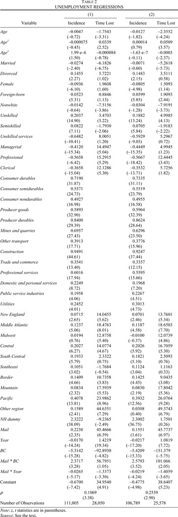
The basic regression results are displayed in Table 2 for two datasets. The first set (the first two columns) includes 111,005 observations, drawn from all those BLS surveys (29) that reported information on unemployment and the complete set of personal characteristics and all census respondents, whether in or out of work on the day of the census.28
Five surveys were excluded because of the absence of information on either nativity (in 1,239 cases) or marital status (in 2,197 cases). Nativity is also not reported for 613 cases in covered surveys, and marital status for a further 577 cases. We test the significance of these missing variables in our sensitivity analysis.
The second (reported in columns 3 and 4) excludes the 4,216 employees who were out of work on the day of the census (for whom outwork equals one). Although there were some differences in the coefficient estimates between the two samples, their signs and statistical significance remained stable, as did the predicted outcomes of the model. The model was also calibrated against other datasets, structured to test the sensitivity of our final results to the specific sample characteristics of the integrated dataset. We find that the core results are stable to quite radical changes in the construction of the dataset.
29 These findings are reported in Table 6.
For now, we begin by examining the outcome of our preferred regression formulation, as displayed in the left-hand columns of
Table 2.
What do these regression results tell us about the structure and nature of unemployment? To begin with, they share with previous analyses of Gilded (and Progressive) Age unemployment the finding that industrial affiliation and place of residence were statistically significant determinants of unemployment. Thus, the probability of becoming unemployed was significantly lower for workers on the railroad (which was chosen as the default as it was the classic stable occupation) than in any of the other designated industries. Unsurprisingly, construction has the highest incidence of unemployment, followed closely by producer and consumer durables; the lowest incidence was to be found among those in trade and commerce, public utilities, and in the domestic-, personal-, and public-service sectors. The range of experience in the other industries was relatively small. Regional location also influenced unemployment, independent of industrial structure. The Pacific states were a high unemployment region; New England and the Midwestern states were among the lowest.
Our results place more emphasis on personal characteristics in determining unemployment than, for example, those of Hatton and Williamson.30
Hatton and Williamson, “Unemployment.”
Here we should distinguish between incidence and time unemployed. Time lost was lower for married than for single or divorced workers; for men than for women; for nonwhites than for whites; and for skilled and semi - skilled workers than for unskilled and service workers. In no case, however, were the measured differences in time lost very large. (For age, for example, the difference in predicted time unemployed between 20 and 40 year-olds was less than one day.) From the incidence equation, we find that women were less likely to lose their jobs (albeit from a much lower level of participation) than men, as were the native-born relative to immigrants, and married workers relative to those single or divorced; race was not a statistically significant independent marker of incidence. Skill levels were (empirically and statistically) the most significant personal determinants of incidence: incidence was highest for unskilled production workers, relative to the default skilled worker, and lowest for service employees.
Moving to survey-specific variables, we see the following. The coefficients on year (which refers to the beginning year and quarter covered by the survey) indicate that although the incidence of unemployment was declining over the late nineteenth and early twentieth centuries ceteris paribus, the average time spent out of work for those who experienced unemployment was slowly rising over the course of the period. Unsurprisingly, the NH (New Hampshire) dummy was large and strongly positive in the incidence equation, although the workers in that survey spent no more time out of work than on average. And finally, responses did vary by survey procedure. We anticipated that mail respondents would be more likely to complain about their employment situation, and would be more responsive to cyclical fluctuations; and so it transpired.31
As a further test of the role of survey procedures, we added outwork to the base equation. Workers who were unemployed on census day tended to have higher incidence and time lost due to unemployment in the previous year, consistent with the positive value of ρ in Table 2.
The most important result for our analysis of the natural rate of unemployment measures the impact of changes in the business-cycle variable, our estimate of the cyclical sensitivity of unemployment in the period between 1880 and 1910. The coefficients indicate that both incidence and time lost varied inversely with the cycle. They also show that cyclical volatility was felt in the labor market primarily by changes in the breadth, rather than the depth, of unemployment. The incidence of unemployment was highly sensitive to cyclical movements, and the elasticity of time lost was very low. Over three-quarters of the total change in nonfarm unemployment in response to a change in the business cycle was accounted for by changes in incidence.32
The attribution of changes in unemployment between changes in incidence and time lost were calculated by total differentiation of the formula for the unemployment rate. Thus, U=I*D, where U, I, and D symbolize the rate of unemployment, the level of incidence, and the average time lost (duration) respectively. Total differentiation yields: ΔU=IΔD+DΔI.
This is a dramatic reversal from the pattern that has developed in the postwar period, in which variations in unemployment are primarily caused by changes in duration rather than incidence.
33 Sider, “Unemployment Duration”; Dynarski and Schefrin, “Behavior”; and Baker, “Unemployment Duration.”
We should also note that, pace Romer, our results indicate a higher level of cyclical volatility of unemployment a century ago than in the recent past. The implied decline in volatility may well be a contributory factor in the trend of the natural rate over the first half of the twentieth century.
THE NATURAL RATE OF UNEMPLOYMENT IN 1909
As noted previously, our estimate of the natural rate of unemployment is structural, being constructed from the regression results of Table 2 by setting the business-cycle index to zero. The procedure is akin to neutralizing the demand and supply shocks to the macroeconomy for a particular year. The natural (equilibrium) rate is calculated for 1909 by simulating the incidence and time lost in unemployment for each observation in the 1910 census public use sample, with the business cycle variable forced to zero. The virtue of using the census year is, of course, that the 1909 observations are self - weighted, so that the census provides the occupational weighting necessary to construct an economy-wide estimate of nonfarm unemployment. It also permits us to determine how far the correction for cyclical location affects the actual levels of unemployment reported in Table 1.
What do these natural-rate estimates tell us about unemployment before 1914? The estimated natural rate for workers in the cyclically sensitive sectors (manufacturing, mining, and construction) is 7.9 percent (compared to the baseline measure of 6.4 percent in Table 1); for all nonfarm civilian employees, it is 5.9 percent (compared to a 5.0 percent baseline).34
All estimates in this and following paragraphs refer to the results from the dataset including workers who were unemployed on census day; they are derived from columns 1–2 of Table 2.
When extended to the entire civilian labor force (by applying the recorded unemployment rate for agricultural workers, and positing full employment for employers and the self-employed), the economy-wide natural rate is estimated to be 4.05 percent, compared with the actual rate, calculated in like fashion, of 3.4 percent.
35 The use of the recorded unemployment rate for agricultural workers in 1909, rather than a constructed natural rate, reflects two concerns, one general and one specific. The specific concern is that there are insufficient data from the BLS surveys on farm workers to allow for proper estimation of a cyclical component applied to this sector. The general issue is that raised by Calomiris and Hanes (“Consistent Output Series,” p. 17), who note that, “Wesley Mitchell, George [sic] Burns, and other National Bureau researchers had shown agriculture to be uniquely acyclical.” It seems safest then to apply the census estimate of unemployment without correction for these workers. To the extent that agricultural employment was cyclically sensitive, our estimate will understate the economy-wide rate. Note also that we follow Lebergott (Manpower, pp. 384–89) in excluding “excess” family workers from the labor force in calculating the overall agricultural rate. We applied the recorded 1909 unemployment rate to those “home-farm” workers retained in the reconstructed labor force.
As noted in the text, the census directed enumerators to record unemployment as a missing value for employers and the self-employed. Once again, to the extent that the self-employed did experience unemployment in 1909, this will bias down our estimates. There is some ground for debate on this point. Thus, Lebergott (Manpower, p. 406, n. 14) makes the case for assuming the same unemployment rate for some self-employed as for their equivalent wage-earners. The Preston sample indicates that, although self-employed artisans did experience unemployment on a similar (though lower) level as employed artisans (e.g., self-employed blacksmiths lost on average 10.6 weeks of work, employed blacksmiths, 14.9 weeks in 1909; self-employed and employed masons lost 31.1 and 35.7 weeks respectively; self-employed and employed carpenters lost 16.6 and 23.9 weeks, etc.), it is nonetheless the case that the number of such artisans was few (less than 3.5 percent of all masons and carpenters), while the preponderance of the self-employed were retail dealers, launderers, dressmakers, doctors, and boarding house keepers. For these groups, an assumption of zero unemployment seems more appropriate.
An estimate of the natural rate at 4 percent in 1910 conforms to previous estimates offered by Robert Gordon and by Richard Vedder and Lowell Gallaway.36
Gordon, Macroeconomics, p. A1; and Vedder and Gallaway, Out of Work, p. 252.
The natural rate appears to have changed little over the first half of the twentieth century: economy-wide estimates for the 1960s also averaged around 4 percent.
37 Summers, “Why is the Unemployment Rate,” pp. 340–43; and Rissman, “What is the Natural Rate.”
There was an apparent upward trend in the natural rate through the early 1990s, when accepted levels were closer to 6 percent, yet recent macroeconomic evidence suggests that the current figure may be lower than that, perhaps as low as 4.5 percent.
38 Motley, “Has There Been a Change.”
But the aggregate picture hides as much, perhaps more, than it reveals. There have, after all, been dramatic structural changes in the composition of the labor force in the past century. Agricultural employment shrunk from 18 percent of the wage-earners in 1910 to below 3 percent by 1950 and less than 1.5 percent by 1980. The proportion of the self-employed, within and outside of agriculture, has also declined sharply—from 29.5 percent in 1910 to 16.5 percent in 1950 and 9.2 percent by 1980. There have also been significant changes across demographic groups: women rose from less than 25 percent of the civilian labor force in 1910 to almost 30 percent by 1950 and over 40 percent by 1980; the share of nonwhite workers in the labor force has likewise risen; and there was a sharp decline in the proportion of the foreign born.
Given the decline in the labor-force share both of agriculture (which has historically recorded lower unemployment rates than the nonfarm sector) and self-employment (for which measurement problems for calculating and interpreting unemployment abound), it seems sensible to focus attention on changes in the unemployment rate among nonfarm employees. Disaggregation of unemployment experience by race and sex also seems appropriate, in light not only of the changing demography of the labor force since 1910, but also in view of the significantly different unemployment history of these groups, as reflected in the coefficients recorded in Table 2. Finally, the recent history of the age structure of unemployment suggests that disaggregating by age may be a further useful point of comparison.
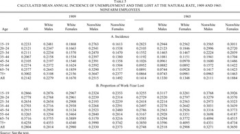
Table 3 thus decomposes the natural rate by age, sex, and race. The calculations are presented for two groups. The upper panel refers to workers in the cyclically responsive sectors (manufacturing, mining, and construction); the lower panel to all nonfarm employees. Comparison with Table 1 suggests that cyclical burdens tended to fall more heavily on workers in the core working years (20–54) than on younger or older workers; at proportionately similar rates by race and sex; and, as one would expect, disproportionately on workers in cyclically sensitive sectors.
How do these results compare to modern experience? To assess this, we employed the same regression methodology to estimate the natural rate for nonfarm employees for 1965, a year similar to 1909 in terms of its location on the business cycle. The data for the regressions were extracted from the individual work experience files of the Current Population Survey, which report the incidence of unemployment and time spent out of work in the year preceding the March interview. A Heckman regression was run over the period 1962–1973, using the same sampling frame and the same variables as in the prewar equation (except for nativity, which was not reported, and mail, which is irrelevant); the same procedure was used to generate an estimate of the natural rate compatible with the 1909 figure. Table 4 reproduces the recorded rates of unemployment in 1965 by age, sex, and race for cyclically sensitive industries and for all nonfarm employees, alongside the estimated natural rates for each group. The measured unemployment rate for nonfarm employees in 1965 was 3.6 percent; the estimated natural rate is 4.05 percent.39
Choosing a year other than 1965 as the reference year for the 1960s makes little difference to our results: the average natural rate for nonfarm employees for 1962–1973 was 4.22 percent; the measured rate, 3.90 percent.
The rates for cyclical sectors are, as would be expected, higher, at 4.3 and 4.7 percent respectively. The implied decline in the natural rate was a little below two percentage points for civilian nonfarm workers between 1909 and the mid-1960s, and around three percentage points for those employed in cyclical industries.
40 This figure may, as one referee has noted, exaggerate the extent of the difference. Workers in agriculture in 1910 may have been risk averse, seeking refuge in stable employment conditions on the farm. By the 1960s, agricultural employment had shrunk and risk-averse workers would have to look elsewhere for stability—perhaps in the government sector. These risk averters would thus have moved from farm to nonfarm employment, thereby pulling down the unemployment rate in the nonfarm sector. Certainly, the growth of stable employment in the nonfarm sector is one aspect of the compositional shifts that shaped the change in the natural rate over time, although we would not wish to exaggerate its impact. After all, the classic stable sector of railroads falls into the nonfarm sector in 1910 and was a significantly larger component of total employment then than in the 1960s.
Comparisons of the demography of the natural rate between the early-and mid-twentieth century, as captured in Tables 3 and 4, reveal significant compositional changes in the structure of unemployment over this period.41
These demographic changes are also reflected in the distribution of measured unemployment in 1909 (see Table 1) and in the work experience survey (see Table 4) and are not simply a result of the transformation to the natural rate.
White males were the major beneficiaries of lower unemployment, with a natural rate in 1965 almost half that of 1909.
42 All of the comparisons made in this paragraph refer to the nonfarm worker estimates for 1909, from panel B in Table 3. Our results for 1965 are similar to G. E. Johnson and P. R. G. Layard's estimates of the natural rate by demographic group (“Natural Rate,” p. 988), which are based on a Barro unanticipated money equation; their unemployment rates for mid-career white males are 2.5 percent in 1955 and 2.8 percent in 1979.
The average natural rate also fell for white females, though to a lesser extent, while it rose for nonwhite workers, especially for nonwhite females. The profile of the natural rate by age also changed: youth unemployment rates were consistently higher in 1965 than in 1909, and elderly unemployment rates consistently lower. Moreover, a similar age-profile, in which the ratio of the natural rates in 1965 and 1909 falls monotonically with rising age, is shown for all age-sex categories.
43 These comparisons apply also to the base unemployment rates generated by the census and the work-experience survey and are thus not a figment created by our technique for moving from the recorded to the natural rate.
These demographic changes can be traced to specific structural and institutional changes in the labor market. Thus, the lower natural rate among older workers reflects the rising importance of retirement in 1965 relative to 1909 (coupled with improvements in health for those still in the labor force); similarly, the much higher levels of youth unemployment in the postwar period were shaped by changes in public policy over the twentieth century, most notably the introduction of the minimum wage, the expansion of tertiary education, and the raising of the school-leaving age. More tentatively, the finding that nonwhite women experienced less unemployment before World War I than since World War II may reflect the decline of domestic service over the twentieth century.44
But note that the results both for females and nonwhites are necessarily tentative. Both were under-represented in the state BLS surveys. The BLS surveys originated primarily in the north-east and mid-western states. The (relatively) low share of blacks in the sample groups is to be explained almost entirely by this geographical bias, as well as the concentration of the surveys on the nonagricultural sector. Women are somewhat better represented in the surveys, but in a very spotty way—they appear in a few of the Michigan surveys (the vehicle workers in 1896, for example), but in next to none of the Kansas or New England reports. This reflects the extent of occupational segregation to be found in nineteenth-century U.S. labor markets; when state bureaus were interested in evaluating women's employment, they undertook special surveys of certain industries. Unfortunately, these surveys almost never reported the individual level information used in this article. The net result of this is that the nonwhite and female employees included in our regressions are dominated by census observations, and show little change between the actual and natural rates. The extent of any downward bias cannot be definitively determined, although external evidence suggests that it is likely to be small.
The rise in retirement and the decline in youth labor also imply that employment weights have changed, suggesting that some part of the falling natural rate may be attributable to the changing demography of the labor force, as the two groups most susceptible to unemployment decline in importance. In order to measure this effect, we recalculated the 1965 natural rate using 1909 employment weights. The re-weighted natural rate for nonfarm employees is 4.64 percent; for cyclical workers, 5.48 percent. The decline in the natural rate is lessened, but it is still clearly apparent. The two-stage procedure followed in the construction of the natural rate also allows us to separate out the influences of incidence and time spent in unemployment. The decomposition is displayed in Table 5. The average length of time spent out of work by nonfarm employees in 1909 was close to three months. Margo and Alexander Keyssar produce similar figures for census years before 1909, thereby supporting our finding that time lost was relatively stable across cycles and over time.45
Margo, “Incidence”; and Keyssar, Out of Work.
About a fifth of the employed labor force lost some time during the year. Whites spent more time out of work than nonwhites; females more time than males. The differences between white and nonwhite are not trivial—they would imply a lower unemployment rate of over 1.4 percent for nonwhite males at the same level of incidence. The difference was somewhat offset by the lower level of incidence of unemployment for white males. The differences here, however, were very small (accounting for less than 0.5 percent of total unemployment); for women, moreover, nonwhites experienced both lower incidence and time lost than whites.
Although the average unemployed worker spent similar periods out of work in 1965 as in 1909, the incidence of unemployment was much lower in the postwar year (14 percent vs. 21 percent). As in 1909, unemployed men in 1965 spent more time out of work than women; nonwhites, however, spent more time out of work than whites in the latter year. Similarly, the incidence of unemployment was higher among nonwhites than whites in 1965, and higher among males than among females—a reversal from the earlier period. A further reversal of interest concerns the shape of incidence and time lost by age: in 1909, the age profile of incidence followed a U-shape, whereas time lost rose monotonically with age; in 1965, the incidence of unemployment rose monotonically with age, whereas time spent out of work exhibited a U-shape profile.
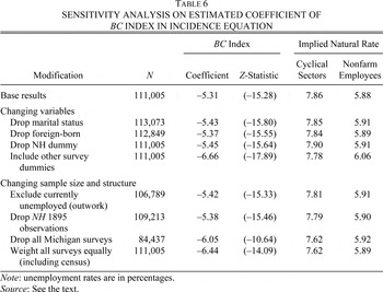
It remains to ask to what extent the results for the prewar period are the product of the artificial structures imposed by data availability. Our dataset has the 1910 Census as its foundation-stone—as reliable a source of historical microeconomic information as might be found—but we recognize that the BLS surveys, as good as they are, are not a representative, random cross-section of all nonfarm employees and were collected occasionally from only a small number of participating states. It therefore behooves us to use sensitivity analysis to ensure that the natural-rate calculations for 1909 are robust and meaningful. We cannot test the sensitivity of our results by drawing another sample from the population of unemployment experiences; however, we can determine how far our results are sensitive to changes within the sample available to us. This we have done by changing the model specification and by changing the datasets. It is not possible to reproduce the complete array of differentiated products; however, in Table 6, we display the range of coefficients (and t-statistics) on the business-cycle variable in the incidence equation, as well as the implied natural rate for nonfarm employees.
It is clear that our results are robust to quite severe changes in the dataset, variable list, and regression methodology. Weighting all surveys equally to remove the influence of the larger BLS surveys and the census; excluding all Michigan observations (to test whether we are nationalizing a Michigan model of unemployment determination); including survey dummies (where statistically significant) in the same format as the New Hampshire dummy46
Surveys identified as having a statistically significant impact on either time lost or incidence were: Maine (1890), New Hampshire (1893), Michigan (1888, 1889, 1895), and Kansas (1895, 1896). The range of coefficients on these dummy variables in the incidence equation was −0.35 to +0.32, compared to a coefficient value of 2.27 for New Hampshire (1896) in the base regression.
; dropping the
NH dummy; dropping the observations for which the
NH dummy equaled one; including the census as a dummy variable; dropping marital status and nativity as variables (in order to increase the number of observations and to extend the range of BLS surveys represented in the regression equation)—none of these specification or dataset changes affected the outcome to any great extent. The range of coefficients on the
BC index was −5.31 to −6.66; the range in the natural rate estimate for nonfarm workers was 5.9 to 6.1 percent; for those in cyclically sensitive sectors, from 7.6 to 7.9 percent. Our results appear stable and consistent.
WHY WAS THE NATURAL RATE SO HIGH IN 1909?
Robert Hall's theory of the natural rate implies that labor markets in which jobs are brief and there are large flows of newly jobless workers have high natural rates of unemployment.47
Does this insight explain the high natural rate in the US non-farm labor market before World War I?
The high rate of labor turnover in American industry, which began to be documented in the decade of the 1910s, was a subject of considerable concern among the economists of the time. And it was indeed high, between two and three times greater in American manufacturing in the early 1910s than in 1960s.48
Slichter, Turnover; Brissenden and Frankel, Labor Turnover, p. 36; and U.S. Bureau of the Census, Historical Statistics, p. 181.
Economic and labor historians are agreed that this was a period of considerable instability in employment.
49 Jacoby, Employing Bureaucracy, pp. 115ff; Whatley and Sedo, “Origins”; and Goldin, “Labor Markets,” pp. 592–96.
There is much less consensus about the causes of high turnover, or its distribution among the labor force. Thus Margo considers unemployment to have been “ubiquitous among the working class,” a judgement echoed by Claudia Goldin's calculation from Kansas BLS data in 1884–1887 that “fully 95 percent of all currently employed Kansas employed laborers would have experienced unemployment” over a period of 3.7 years.
50 Margo, “Labor Force,” p. 242; and Goldin, “Labor Markets,” p. 595.
By contrast, Sanford Jacoby and Sunil Sharma characterize the pre-1914 labor market in “dual labor market terms: … a majority of blue-collar workers and jobs were unstable, but there existed a small sector where workers held quasi-permanent jobs.” Contemporary commentators also noted the bifurcated nature of jobs and turnover, but in almost diametrically opposite terms. Sumner Slichter, on the basis of considerable empirical analysis carried out for the U.S. Commission on Industrial Relations, reported that “turnover is a highly concentrated phenomenon … the high turnover rate in most plants is due to a few men changing rapidly while the great majority of the labor force is stable … turnover is concentrated among a relatively small proportion of the force.” Similarly, Paul Brissenden and Emil Frankel, who headed the official analysis of labor turnover for the Federal BLS, concluded that “inordinate shifting of labor is characteristic only of certain parts of the working force.”
51 Jacoby and Sharma, “Employment Duration”, p. 170; Slichter, Turnover, p. 43; Brissenden and Frankel, Labor Turnover, p. 142.
There is also disagreement over the sources of turnover, and the balance between quits, layoffs, and dismissals. In her recent review of labor markets in the twentieth century, Goldin emphasizes the role of involuntary separations in creating an environment of “considerable job insecurity”; similarly, Margo notes that “economic historians believe that the risk of layoffs was widespread” around 1900, making no mention of quits as a source of high turnover.52
“It is clear that the vast majority of manufacturing workers in most of the states surveyed lost time during the year because they were laid off or were terminated” (Goldin, “Labor Markets,” p. 596). Margo, “Labor Force,” p. 242.
Jacoby, by contrast, locates employment instability in the prevalence of both “high quit and dismissal rates in industrial firms,” observing that while “discharges were meted out liberally” by industrial foremen, quits were frequently used by both skilled and unskilled workers as a means to escape the rigors of factory life.
53 Jacoby and Sharma, “Employment Duration,” p. 172; and Jacoby, Employing Bureaucracy, p. 21, and “Industrial Labor Mobility,” pp. 264–67.
The statistics collected by contemporaries underline the importance of voluntary separations—Brissenden and Frankel report that quits accounted for about three-quarters of all separations, with discharges and layoffs representing 15 and 10 percent respectively.
54 Brissenden and Frankel, Labor Turnover, p. 80. Woytinsky's compilation of turnover statistics reports between 7.3 and 11.3 job separations per 100 workers between 1910 and 1913. (Three Aspects). If we combine the April 1910 figure of 17.75 separations with the recorded (census) unemployment rate of 5.23 percent for 15 April, the implied average completed spell length of unemployment is 7.7 days—very much lower than the aggregated numbers of days lost over a typical year.
These quits, it was argued, were concentrated among “floaters,” who moved from one briefly held job to another, with short periods of unemployment between each one. Given the lack of any funds to underwrite search, such quits would seem to have been unnecessarily risky, were it not for the state of the labor market for unskilled labor, in which new job openings were evidently not so hard to find after a few days tramping.
55 Jacoby, Employing Bureaucracy, pp. 33–37; and Sautter, Three Cheers, p. 53.
Frequent quits produced a high level of demand for new workers, maintaining a high rate of turnover, albeit concentrated among a small segment of the labor force.
56 Part of the difference between these interpretations may be attributed to the empirical evidence used. Thus, Goldin and Margo drew many of their conclusions from an analysis of state BLS data, which were derived from interviews with workers. As we have noted, these surveys tend to be biased towards currently employed workers and against the itinerant labor force, who were responsible for a large proportion of the quits. The data collected by Slichter and the federal BLS after 1910 were drawn from employers and therefore are immune to this criticism. But here too, we have to be careful. To the extent that quits were dominated by “floaters” experiencing multiple short spells of unemployment over the course of the year, these data will overstate the proportion of time spent out of work originating in quits.
Contemporary opinion thus concurs with Hall's theory, with its emphasis on rapid turnover and “frequent short spells of unemployment.”
But we should be careful not to overstate the importance of rapid turnover as the source of a high natural rate. The best empirical evidence available to us for the pre-1914 period is the 1910 Census, which, by covering the currently unemployed, is largely immune to the bias against “floaters” presented by the state BLS surveys. The distribution of total unemployment by months in 1909 (the accumulated duration of all spells for nonfarm employees) is shown in Figure 1.57
The emphasis is designed to draw attention to the confusion inherent in some of the discussion of comparisons of spell length over time. Thus, when Margo (“Labor Force,” p. 242) notes that “by modern standards, the length of a spell of unemployment (in c. 1900) was … relatively brief” (a comment echoed by Goldin, “Labor Markets,” p. 592), the comparison depends crucially on the extent of multiple spells then and now. Total time spent out of work was 3.2 months in 1910, compared to 2.86 months in 1969, 3.46 months in 1974, and 4.37 months in 1975 (Clark and Summers, “Labor Market Dynamics,” p. 36). If all spells in 1910 were singulate (as suggested in Margo, “Incidence”), the average duration in 1910 would have been 3.2 months, compared to 1.42 months in 1969, 1.94 months in 1974, and 2.22 months in 1975 (Clark and Summers, “Labor Market Dynamics,” p. 19). Only if there were multiple spells in 1910 (as there were in 1969–1975) does the Margo-Goldin position hold.
The shape of the distribution militates against an interpretation based wholly on multiple short spells of unemployment: if each single spell of unemployment were brief, we would expect to see many more employees with only a small number of days lost over the course of the year than actually show up in the data.
58 It is possible that the census underreports unemployment at the left tail of the distribution. Thus, Woytinsky (Three Aspects, pp. 15–16) argued that workers were unlikely to report short periods without work, judging it to be search rather than unemployment; recall bias is also likely to be more evident in cases of brief spells.
Moreover, unemployment incidence in the census does not vary significantly by skill, whereas contemporary data indicate that floating was concentrated largely among unskilled workers.
59 The Federal BLS defined unstable workers as those who were employed for less than one year. In a sample of firms in 1913–1915, 44.3 percent of unskilled and semiskilled workers fell into this category, compared to 25.6 percent of skilled workers. The separation rate for the same period among unskilled workers was 1.4 per full-time employee per annum, compared to 0.66 for skilled workers. Quits account for a similar proportion of all separations for both groups. Brissenden and Frankel, Labor Turnover, pp. 158, 191.
Despite these reservations, it seems clear that a comprehensive model of the pre-1914 labor market must incorporate the experience of floaters. Figure 1 cannot be easily reconciled with a model in which unemployment was a pure lottery and all workers were homogeneous. Under such conditions, we would expect the cumulative distribution of unemployment to map out a smooth exponential curve, rather than the shape depicted in Figure 1, which fits better with a heterogeneous model of unemployment. The simplest heterogeneous model is the bifurcated or dual labor-market model suggested by both contemporary analysts and Jacoby and Sharma.60
Jacoby and Sharma, “Employment Duration.”
The empirical issue is to determine the proportion of stable and unstable workers in the labor force before 1914 and to reconstruct the parameters of labor-market separation and accession. To this end, we have adopted a simulation strategy to recreate the distribution of unemployment at the 1910 Census, as shown in
Figure 1.
The simulation procedure predicts the unemployment experience of 10,000 workers, separated into two groups (stable and floaters). A certain proportion of each group is unemployed at the beginning of the year. In each of the 104 bi-weekly periods that follow, unemployed workers have a probability of returning to employment (the accession rate), while those in employment have a probability of losing their jobs (the separation rate). All terminations are treated the same: there is no distinction between quits, layoffs, and discharges. There is homogeneity within the two groups, such that each stable worker is faced with the same separation and accession rates; obviously, the rates are higher for floaters than for stable workers. The diagram shows the proportion of workers who experience at least two weeks of unemployment (periods of unemployment being centered on the nearest whole month); workers who spend fewer than two weeks out of work are excluded in order to make the differences between the models clearer.
The first model implicitly treats all workers as homogenous, by setting one separation rate for all nonfarm employees. It is a steady-state model, for which the accession rate is determined by the usual relationship between the separation and unemployment rates. The model thus requires only two parameters (the unemployment rate and the separation rate), both derived directly from the census.
The second model formally distinguishes stable and unstable workers; each group is assigned a different (average) separation rate. The simulation is modeled in a non-steady-state framework, by setting the accession rate (for stable workers) so that the unemployment rate falls across 1909 consistent with the pattern of cyclical responsiveness analyzed earlier in the article (the model maintains a steady-state assumption for the floaters). This second model is considerably less parsimonious than the first, requiring the specification of six parameters: the proportion of stable and unstable workers in the labor force; the average unemployment rate of each group; the separation and accession rates for stable workers; and the separation rate for floaters. The difficulty is, of course, in the identification of the parameter values. Our approach has been to begin with the estimates provided by Wladimir Woytinsky for the pre-1914 labor market and then to manipulate the parameters iteratively to produce the closest fit to the census distribution of months of unemployment, as determined by a chi-square test statistic of goodness-of-fit.61
Woytinsky, Three Aspects, p. 27. The parameter values in our best-fit bifurcated model are (with Woytinksky's values in parentheses): stable workers: unemployment rate, 4.4 percent; monthly separation rate per employed worker, 0.0091 (0.0178); monthly accession rate per unemployed worker, 0.2064; floaters: unemployment rate, 20 percent; monthly separation rate, 0.5 (0.335).
The distribution of months lost in 1909 as predicted by these two models is shown in Figure 1, alongside the actual data from the census. The homogenous model produces a well-behaved unemployment distribution, in which the proportion of unemployment by month declines smoothly from the first to the eleventh month. The model captures the distribution at the mean duration level (four months) precisely, but is much weaker in its fit with the rest of the distribution. The bifurcated model, by contrast, manages to mimic the entire distribution quite well.62
Note that we have not, for reasons of visual clarity, included the proportion of the labor force that was fully employed for the entire year. The bifurcated model produces an almost precise fit to the census data, whereas the homogenous model slightly underestimates the actual figure.
The chi-square statistics for the two models are 195.3 and 80.5 respectively, indicating the superiority of the heterogenous model across the year as a whole. The largest weakness of the bifurcated model is in months three (which it overstates) and four (which it understates), but this may in part reflect the difficulty in identifying whether workers who declared themselves out of work for 13 weeks should be placed at the end of the first quarter or the beginning of the next.
The simulation approach may also be used to predict the distribution of unemployment spells as well as the cumulative duration of joblessness over the year.63
The simulation may also be used to predict the distribution of employment spells; this allows us to respond to a challenge laid down by Jacoby and Sharma (“Employment Duration”), who rightly argue that censored job distributions give us a biased sense of the extent of lengthy job tenure in the labor market. In the interests of space, we have postponed the analysis of tenure for another paper.
The homogenous model predicts that 95 percent of unemployed workers experienced only one spell; the average spell length was, in consequence, only marginally less than the average duration of joblessness over the year. In the bifurcated model, in contrast, multiple spells are more frequent, affecting fully a third of workers who become unemployed. The average number of spells is 2.2 per unemployed worker, with an average spell length of 1.63 months. The average mediates between two groups with dissimilar unemployment profiles. The simulation model predicts the mean unemployment spell length of floaters at 0.54 months, with an average of 5.1 spells a year. All but 5 percent of stable workers in the simulation experienced single spells, of about 3.95 months on average.
Certain inferences may be drawn from the simulations. Firstly, the bifurcated model is clearly superior to the homogeneous model in its ability to capture the distribution of unemployment.64
The bifurcated model is also compatible with the turnover data before 1914, whereas the homogenous model is not. The monthly separation rate implied by the latter model is 0.0156 per employed worker; the rate for the bifurcated model is 0.037, identical to the rate reported by Woytinsky (Three Aspects, p. 27) for 1913–1914, properly weighted between stable and casual workers.
It is not perfect, suggesting that there would be some room for complicating the model still further—perhaps by having more than two groups, perhaps by introducing some degree of duration dependence among nonfloaters. But these would be minor revisions. Second, the balance between stable and unstable workers conforms more closely to contemporary estimates than to the proportions suggested by Jacoby and Sharma. Rather than the labor market being dominated by casual workers, with a small core of stable employees, the simulations suggest that only about 6 percent of workers are properly defined as floaters.
65 Woytinsky estimated that floaters were 11–12 percent of the industrial labor force. But note that his data focused primarily on manufacturing workers, whereas our estimate of 6 percent refers to all nonfarm employees.
We also employed a switching regression methodology to estimate the proportion of floaters in the population. The strategy begins by assuming that the floaters would be concentrated among those out of work less than three months in 1909, and that they could be identified with reference to their age, sex, race, nativity, and skill, as well as their unemployment experience on the day of the census. The switching regression ground out an estimate (mean probability) of being a floater of 6.25 percent of nonfarm employees.
Clearly, the distinction between stable and unstable workers is to a significant extent a matter of definition. Thus, Brissenden and Frankel define unstable workers are those who remain attached to a firm for less than one year; whereas Jacoby and Sharma seem to have in mind “lifetime jobs” when referring to stable workers (although their analysis of unstable workers focuses on job tenures of less than a calendar year). It may be then that the bifurcated model is not a fit test of the Jacoby-Sharma interpretation, and that a third category of highly stable workers may be a necessary further adornment.
Third, although floaters are a small proportion of the labor force, they are responsible for 68 percent of all unemployment spells. To the extent that separation rates for floaters took the form of quitting, whereas more stable workers were more liable to be separated by layoff or dismissal, this is consistent with the data from the federal BLS, which measured the proportion of quits as 75 percent of all separations. Fourth, and following from this point, it seems evident that quits rather than layoffs and discharges dominated labor turnover in the pre-1914 marketplace.
66 This was certainly the case in the 1920s; between 1919 and 1929, the quit rate was higher than the layoff rate in 127 out of 132 months. Only during the depression of 1920/21 and in December 1929 was the layoff rate higher. For the remainder of the period, quits were more than three times as important as a source of job separation as layoffs and discharges combined. Woytinsky, Three Aspects, pp. 228–29.
The emphasis placed on layoffs by Goldin and Margo seems misplaced, other than for severe downturns (such as the 1890s) when they were likely to have dominated separations.
67 There is no direct evidence on the balance of quits and layoffs during the 1890s. But the evidence from 1920/21, plus the cyclical volatility of both quit rates and layoff rates during 1910–1920, suggests that the share of quits in total separations would have been lower during depressions. Note, however, that even in the November 1920–March 1921 period quits accounted for 38 percent of total separations (ibid.). Moreover, some proportion of those layoffs would have been temporary rather than permanent, while the discharge rate shows counter-cyclical behavior, consistent perhaps with improved employment performance and lower absentee rates during downturns and slumps.
Fifth, it appears necessary to qualify Margo's conclusion that “by modern standards, the duration of a spell of unemployment was … relatively brief.” The mean duration of a completed spell in 1969 was 1.42 months; for an “indomitable” job seeker (i.e., excluding the effects of withdrawal from the labor force), it was 2.03 months. These are lengthier spells than for floaters, but shorter than for stable workers.
68 Margo, “Labor Force,” p. 242; and Clark and Summers, “Labor Market Dynamics,” p. 19.
The simulations make it clear that Hall's theory, with its emphasis on rapid turnover, provides an important clue to our understanding of the high natural rate before 1914. The bifurcated model indicates that, in the absence of floaters, the reported unemployment rate in 1909 would have fallen from 5.3 to 4.4 percent (given the high sensitivity of casual unemployment to the business cycle, the contribution of floaters would have been greater at the natural rate).69
It should be noted that the census data relate to a better than average year; consequently, it is not possible to derive conclusions about the distribution of unemployment at the natural rate. It would be possible to simulate conditions at the natural rate, if it were possible to capture the appropriate separation and unemployment rates for the two groups (as the natural rate is a steady state, we would not need separate accession rates). Unfortunately, we do not have enough evidence to sustain such an approach. The Federal BLS surveys of firms in 1913/14 and 1917/18 indicate considerable cyclical sensitivity in the separation rates of both stable and unstable workers. In the earlier year, marked by stable employment, the monthly separation rate for stable workers was calculated by Woytinsky (Three Aspects, p. 27) at 1.8 percent; in the boom year of 1917/18, with sharply increasing employment, the rate rose to 3.4 percent per month. A similar pattern emerged among the unstable group, with monthly separation rates rising from 33.5 percent to 70 percent across the boom. The implication is that the contribution of floaters to unemployment would be lessened at the natural rate; the balance of separations would move towards the stable workers. To the extent that Woytinsky's data exaggerate the level of quits among stable workers, to the detriment of layoffs, the shift in balance between the two groups would be greater. This conclusion is emphasized by the clear counter-balancing behavior of quits and layoffs over the business cycle, as shown in Brissenden and Frankel (Labor Turnover, p. 83).
It is the presence of floaters that accounts for the greater role of incidence in shaping the responsiveness of unemployment across the business cycle before 1914 than since 1945. But attention also needs to be focused on the unemployment experiences of the stable workforce, most notably with respect to spell duration, which was clearly higher before 1914 than in the 1950s and 1960s.
One possible explanation for a longer spell duration among stable workers before 1914 is the greater extent of seasonality then than now.70
The seasonality of employment flows was a subject of great interest to economists at the time (e.g., Feldman, Regularization), but it has attracted little attention from economic historians (one exception being Engerman and Goldin, “Seasonality”).
It was not uncommon for industries to exhibit considerable seasonal variation in employment.
71 Woytinsky (Employment, pp. 21–22, 36–38, 55–57) provided data on the seasonality of separations which showed that seasonality was less important in the 1920s and 1930s than before 1919; and that the nature of seasonal separations was changing, with layoffs becoming gradually more important than quits.
Seasonal lulls arose from both the supply and demand side. On the demand side, such products as ice and processed fuel showed clear seasonal trends, as did certain clothing lines. But of more significance were supply sources of seasonal fluctuation. These were associated with the nature of the product, or the nature of the production process. Food processing was highly seasonal (fruit and vegetable canning was among the most volatile of all industries), as was fish curing and canning. So too were those industries which depended on water power. Freezing in the winter and low stream and river levels in the summer often meant that mills and factories had to close down for long periods without power. A number of other industries shut down at the height of summer in response to heat—glassworks would close because of the impact on workers; confectionery producers because of the impact on the product.
72 The exact empirical relationship between seasonality and the natural rate can only be sketched out at this stage. We are currently examining the extent and pattern of seasonal unemployment over the period 1890–1920, using payroll records collected by the New Jersey and Massachusetts Bureaus of Labor Statistics, in order to determine how far seasonal variations were key to understanding the higher natural rate.
A further source of temporary dislo-cation came from the unstable course of production itself, apart from seasonal factors.
Evidence from the Censuses of Manufactures indicates that shutdowns (whether for seasonal or other reasons) may have contributed significantly to unemployment at the beginning of our period. Thus, in 1880 manufacturing establishments employing 40.2 percent of workers operated on a part-year basis (at least one month of the year on three-quarters time or less); the average time out of operation for part-year producers was 3.51 months.73
A further 13–14 percent of full-year establishments engaged in “short-time,” with consequent short layoff spells for employees. Atack, Bateman, and Margo, “Part-Year Operation,” p. 797, n. 18.
Not every shutdown would be associated with seasonality—business cycle as well as idiosyncratic factors (fire, refitting, maintenance, closure due to death or bankruptcy of the owner) are other sources—but it is interesting that small rural establishments were most likely to have shut down during the year, consistent with a seasonal explanation emanating from the impact of agriculture on local labor supplies and from inconsistent sources of power. Further, seasonality need not result in shutdowns. Thus, the Census of Manufactures in 1880 reported that 34 out of 211 glassworks closed down during the year, of which 23 were idle all year, having (the Census Office surmised) gone out of business completely. Yet glass production was among the most highly seasonal industries in terms of its monthly employment pattern. In such capital-intensive industries, seasonality may not have led to shutdowns, but to the release of a certain proportion of the labor force, as firms tried to cover part of their fixed costs by producing at a lower level.
There are two further caveats to an emphasis on shutdowns as a source of a high natural rate. First, they seem likely to have been more important in manufacturing than in other sectors of the nonfarm economy (e.g., transportation, trade, and other services) throughout the late nineteenth century. Moreover, they declined in importance within manufacturing over time as the increasing capital intensity of production and the replacement of waterpower by steam and electricity reduced the incentives for plant closures.74
To test this hypothesis, we ran a regression of reported days in operation by manufacturing firms (Rees, Real Wages, table 10) on a business-cycle index derived from Frickey's industrial output index (GAP) and a time trend from 1890–1914. The results were as follows (t-statistics in parentheses): DAYS=−691.03 (−2.40)+72.35 GAP (7.08)+0.51 TIME (3.45); R2=0.677. We ran a variant which included the data from the Census of Manufactures in 1870 and 1880; the revised regression results were: DAYS=−652.72 (−3.31)+73.47 GAP (7.55)+0.49 TIME (5.00); R2=0.725. The addition of an interactive variable combining GAP and TIME provided weak support for the hypothesis that the cyclical responsiveness of days in operation was also declining over the period.
Increasingly, firms responded to cyclical downturns in demand for their products by practicing selective temporary layoffs for stable workers.
75 Thus, the higher coefficient on unskilled in the incidence equation (Table 2) reflects both the concentration of floaters among the unskilled and the tendency for firms to hoard skilled workers during cycle downturns and temporary dislocations.
Businesses in the late nineteenth century produced almost overwhelmingly to order; they did not accumulate stocks to carry them from one season to another.
76 Abramovitz, Inventories; and Zarnowitz, Orders.
Employment was consequently quite variable. Many firms did not follow the practice of formally discharging workers during these lulls; instead, they placed them on temporary furlough, with instructions to wait until they were recalled.
77 Alexander's analysis of engagements by 12 engineering firms in 1912 indicated a monthly turnover rate of 6.5 percent; and that rehires accounted for 37 percent of engagements over the year (Florence, Economics of Fatigue, pp. 138–40).
Don Lescohier, for example, distinguished between a core of steady workers with the firm who were rarely out of work and a second group of workers who were rehired whenever business picked up and let go when “jobs” ran low.
78 Lescohier, Labor Market, p. 58. He also mentions a third group, close to the reserve army of the unemployed, who were employed irregularly during the busy season and not at all during the slack season.
Workers accepted these periodic layoffs as part of their employment relation with the firm, either because search costs were too high, or because they were glad to have a few days of “enforced” leisure (aspects of the same issue). As John R. Commons reported in 1925, “workers are not anxious to accept some other kind of work, at an almost inevitable reduction in wages, for if they do they will not be around when employers begin to hire men ‘in the right line’.”
79 Lewisohn et al., Can Business, p. 91.
CONCLUSIONS
On the basis of the limited evidence currently available, it is hard to resist an eclectic interpretation of why unemployment was so high at the natural rate. Seasonal unemployment for some; interruptions between short spells of semi-casual work for others; the need for firms working to order to “carry on [their] payrolls a larger number of workers than can be afforded steady work all the time” accounting for layoffs for others.80
Lauck and Sydenstricker, Conditions, p. 155.
The simulations suggest that the pattern of unemployment at the natural rate was a mixture of short spells and longer spells; the shorter spells due to periods of tramping for the casual unskilled, and temporary furloughs for the regularly employed; the longer spells due partly to seasonality and partly to longer layoffs for marginal workers among the labor pool. The evidence suggests that quits dominated layoffs and discharges in the Progressive era, and were largely responsible for the high degree of turnover characteristic of the period. Turnover was not only high, but also highly variable. This is consistent with our finding that unemployment dynamics before 1914 emphasized changing incidence of unemployment, rather than varying proportions of time lost. The combination of a high natural rate and significant cyclical volatility thus militates against any simplistic interpretation of the U.S. labor market before 1914 as some idyllic “Golden Age” of high flexibility and low unemployment.
Appendix 1: Unemployment in 1909
The Census Bureau did not publish any unemployment figures from the 1910 census schedules until 1948. The 1948 compilations were in the form of “distributions of unemployment for unemployed wage-earners 16 years and over by duration of unemployment.” Lebergott converted these imperfect data into an estimate of aggregate unemployment using the following steps:
- The level of reported unemployment was reduced “to exclude unemployment that would not be counted by current definitions,” using data on types of joblessness retrieved from a federal survey of the cost of living in 1901.
- This reduced level was then “adjusted upward for underenumeration,” using data on unemployment collected by the federal Immigration Commission. The commission reported much higher levels of unemployment incidence in 1909 than did the census, implying a considerable downward bias in the census estimates. The Immigration Commission clearly did not survey all industries and occupations; however, “all major mining and manufacturing industries” were included, and Lebergott considered the results sufficiently representative to convert the aggregate unemployment rate using the ratio of the Immigration Commission figures to the unadjusted census estimates. This correction produced the final estimate of unemployment for nonfarm employees.
- To this figure, Lebergott added an estimate of the unemployment experience of those workers who were self-employed on the day of the census, but who had been out-of-work employees in 1909. “The sum of the two figures then gives the 1910 [sic] unemployment benchmark.”81
Lebergott, Manpower, pp. 405–06.
There are a number of reasons not to accept Lebergott's revisions. We take each of his steps in turn.
- The correction of the 1910 data for including days of nonemployment due to “e.g., no work wanted, drunkenness, old age, strike, vacation” is unnecessary. Enumerators were instructed to exclude, “those who are on a strike, those who are voluntarily idle, those who are incapacitated for any work, or those who are on sick leave or on a vacation.”82
U.S. Bureau of the Census, Instructions, p. 38, para. 177.
- The correction for census underenumeration is likewise inappropriate. It is certainly true that the Immigration Commission reported much higher incidences and durations of unemployment than did the census. It may be true that “a detailed inquiry into family economic status” generally produces “a much more careful consideration of unemployment status during the previous year than would normally occur during the brief census interview.” However, what is demonstrably not true is Lebergott's assertion that the commission “provided data on duration of employment for 220,000 male wage-earners (age 18 and over) in a broad range of industries” in 1910.83
Lebergott, Manpower, pp. 405–6.
U.S. Immigration Commission, Immigrants, vol. 1, p. 134
U.S. Immigration Commission, Immigrants, vol. 1, p. 14; Thorp, Business Annals, p. 214.
Lebergott, Manpower, p. 406.
The percentages were calculated from U.S. Commissioner of Labor, Eighteenth Annual Report, pp. 294–95, cols. 1–12.
- We concur with Lebergott's third step, but note that it affects only a very small proportion of the labor force. In the 1/250 sample, there were 212 individuals who declared themselves self-employed on the day of the census and who indicated some unemployment experience in 1909. The total number of gainfully employed nonfarm individuals in the Preston sample is 103,914.
- Finally, note that Lebergott's corrections are also contradicted by the direct evidence of unemployment on the day of the census. As with the retrospective question, interviewers were told to “ascertain the amount of enforced unemployment,” indicating no need for correction as in step 1. There is also no evidence, nor any reason to believe, that workers systematically understated unemployment on the census day, for reasons of retrospective bias or lack of corroborative evidence, as recommended by step 2. Step 3 is trivial. How then should we explain the discrepancy between Lebergott's estimate of 11.6 percent for nonfarm unemployment in 1910 and the census estimate of 5.28 percent? It seems abundantly clear that Lebergott's figure is significantly overstated.
We would like to thank Stan Engerman and Chris Hanes for very useful comments and suggestions on earlier drafts, as well as anonymous referees and discussants and seminar participants at the AEA meetings, St. Antony's College, Oxford, Universidad Carlos III Madrid, University of Melbourne, and Australian National University. Ted Kilsdonk provided excellent research assistance early on. Responsibility for any errors or omissions may rest with the authors.