1 Introduction: from impact to sheet expansion
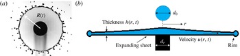
The fragmentation of drops upon impact on surfaces is ubiquitous in nature and industry. Depending on the relative magnitude of the inertial and viscous to interfacial forces involved, the impact can result in a drop deposition, a bounce or a splash. In the latter case, upon collision, the impacting drop crushes and forms a radially expanding sheet. This sheet, in turn, can produce secondary droplets (e.g. figure 1 a). Understanding the physics governing the impact and fragmentation processes has significant implications for the control and optimization of a wide range of industrial operations in lithography (Banine, Koshelev & Swinkels Reference Banine, Koshelev and Swinkels2011), surface coating (Rein Reference Rein1993), ink jet printing (Zable Reference Zable1977) and pesticide spraying (Bergeron et al. Reference Bergeron, Bonn, Martin and Vovelle2000). It is also becoming clear that elucidating the physics governing fluid fragmentation is also vital to understand, predict and control the transport of pathogens shaping disease transmission (Bourouiba & Bush Reference Bourouiba, Bush and Fernando2013; Bourouiba, Dehandschoewercker & Bush Reference Bourouiba, Dehandschoewercker and Bush2014; Gilet & Bourouiba Reference Gilet and Bourouiba2014, Reference Gilet and Bourouiba2015; Bourouiba Reference Bourouiba2016; Scharfman et al. Reference Scharfman, Techet, Bush and Bourouiba2016).
(a) Expanding sheet and (b) associated schematics.

Despite the increasing attention paid to drop impact on solid surfaces since its first description by Worthington (Reference Worthington1876), a unified predictive theory of impacts is still missing (Josserand & Thoroddsen Reference Josserand and Thoroddsen2016). The full description and mathematical modelling of the impact process from touch down to secondary droplet ejection requires an understanding of the sheet creation, expansion and destabilization (figure 1
a). Most studies focus on the prediction of the maximum radius of spreading. One key remaining knowledge gap preventing comprehensive modelling of impact and prediction of fragmentation is the spatio-temporal thickness profile of the radially expanding sheet (Yarin Reference Yarin2006; Roisman, Berberovi & Tropea Reference Roisman, Berberovi and Tropea2009; Josserand & Thoroddsen Reference Josserand and Thoroddsen2016). In this paper, we focus on elucidating the unsteady sheet thickness profile expanding radially in the air from the impact on a surface of comparable size to the impacting drop. Such a profile is both of fundamental importance (Savart Reference Savart1833; Worthington Reference Worthington1876; Taylor Reference Taylor1959; Eggers & Villermaux Reference Eggers and Villermaux2008) and of practical importance to control plant spraying and pathogen transmission (Gilet & Bourouiba Reference Gilet and Bourouiba2014, Reference Gilet and Bourouiba2015). In particular, we focus on the experimental configuration illustrated in figure 1, where the impacting drop forms a radially expanding sheet in the air. This unsteady dynamics is governed by two dimensionless parameters: the Weber number,
 $We=\unicode[STIX]{x1D70C}u_{0}^{2}d_{0}/\unicode[STIX]{x1D70E}$
and the Reynolds number,
 $Re=\unicode[STIX]{x1D70C}u_{0}d_{0}/\unicode[STIX]{x1D707}$
, where
 $u_{0}$
is the impacting speed,
 $d_{0}$
is the impacting droplet diameter,
 $\unicode[STIX]{x1D70E}$
is the surface tension of the impacting fluid,
 $\unicode[STIX]{x1D70C}$
is the density of the fluid and
 $\unicode[STIX]{x1D707}$
is its viscosity. We focus our attention on high
 $Re$
and
 $We$
impact regimes. In this regime, two groups proposed mathematical models of sheet expansion (Rozhkov, Prunet-Foch & Vignes-Adler Reference Rozhkov, Prunet-Foch and Vignes-Adler2002, Reference Rozhkov, Prunet-Foch and Vignes-Adler2004; Villermaux & Bossa Reference Villermaux and Bossa2011). The proposed models have many similarities but also fundamentally differ in the postulated expanding sheet thickness profile: one group conjectured the thickness profile to be
 $h_{R}(r,t)\sim t/r^{3}$
(Rozhkov et al.
Reference Rozhkov, Prunet-Foch and Vignes-Adler2004) and the other to be
 $h_{V}(r,t)\sim 1/rt$
(Villermaux & Bossa Reference Villermaux and Bossa2011), where
 $t$
is time, and
 $r$
is the radial position from the impact point (figure 1). These profiles were not verified until recently when Vernay, Ramos & Ligoure (Reference Vernay, Ramos and Ligoure2015) provided direct measurements of the sheet thickness profile. They reported that the sheet thickness appears to follow the profile
 $h_{R}(r,t)$
at early times
 $t\ll \unicode[STIX]{x1D70F}=d_{0}/r_{0}$
while following the profile
 $h_{V}(r,t)$
at later times
 $t\gg \unicode[STIX]{x1D70F}$
; thus suggesting that both profiles are partially correct. Finally, in all these prior studies, discrepancies emerged on the maximum radius of the sheet. The discrepancies were attributed to the different experimental conditions used. In particular, inconsistent choices of surface-to-drop size ratios was noted. We define
 $\unicode[STIX]{x1D702}=d_{r}/d_{0}$
as the ratio of surface-to-drop diameter. The values of
 $\unicode[STIX]{x1D702}$
used in prior literature ranged from
 $\unicode[STIX]{x1D702}=1$
in Villermaux & Bossa (Reference Villermaux and Bossa2011) to
 $\unicode[STIX]{x1D702}=1,1.39$
in Rozhkov et al. (Reference Rozhkov, Prunet-Foch and Vignes-Adler2002) and
 $\unicode[STIX]{x1D702}=1.67$
in Vernay et al. (Reference Vernay, Ramos and Ligoure2015). The effect of
 $\unicode[STIX]{x1D702}$
on the expansion remains an open question.
In this paper, we have four objectives. First, we return to the governing equations of motion to revisit the modelling of radially expanding sheet and derive, from first principles, the self-similar solution governing its expansion in the air. Second, we use the derived expression to plot the experimental results by Vernay et al. (Reference Vernay, Ramos and Ligoure2015) and show that the seemingly distinct curves reported therein all collapse onto a master curve: our derived self-similar solution. Third, we propose a unified functional form of the sheet thickness
 $h(r,t)$
that allows us to unify the expression for the unsteady sheet profile for all times and thus reconcile the two proposed theoretical forms,
 $h_{R}(r,t)$
and
 $h_{V}(r,t)$
, conjectured in the literature thus far. Fourth, we report our experimental results of direct and indirect measurements of sheet thickness profiles, and the direct measurement of the velocity profile within the sheet as a function of the surface-to-drop size ratio. We show excellent agreement with our proposed profile over an optimal range of surface-to-drop size ratio and elucidate the optimal range in light of the boundary layer on the surface. We also provide the physical interpretation of all the constants in the proposed unified thickness profile and confirm such an interpretation from multiple methods of measurements of thickness and velocity. Finally, our results quantitatively link the fluid history on the surface to the thickness and velocity profiles of the freely expanding sheet in the air.
2 Theoretical background on sheet expansion
2.1 Governing equations and key role of the sheet thickness profile
To understand the impact dynamics and its resulting expansion in the air (figure 1) an equation governing the sheet radius
 $R(t)$
is required. Figure 1(b) is a schematic of the expanding sheet from impact of a drop of diameter
 $d_{0}$
and initial volume
 $\unicode[STIX]{x1D6FA}_{0}$
showing the axisymmetric and thin sheet. Each sheet cross-section can be averaged in the vertical,
 $z$
, direction. This averaging and slender shape allow us to express the sheet velocity
 $\boldsymbol{u}(r,t)$
and thickness
 $h(r,t)$
profiles as independent of
 $z$
. Moreover, the entire rim can be viewed as a control volume. During the expansion, the fluid in the sheet moves radially away from the rod, and accumulates in the rim (Villermaux & Bossa Reference Villermaux and Bossa2011), which is decelerated by the interfacial forces of the sheet. The radius of the sheet
 $R(t)$
can be described from momentum and volume conservation. However, they are not sufficient to solve for
 $R(t)$
. The sheet velocity
 $u(r,t)$
and thickness profiles,
 $h(r,t)$
, are also required and missing.
Returning to the quasi-two-dimensional momentum equations, the high
 $Re$
considered herein allows us to neglect viscous and compressibility effects in the sheet. Similarly, curvature-induced radial pressure gradients in the sheet are neglected (Yarin & Weiss Reference Yarin and Weiss1995), thus leading to
 $$\begin{eqnarray}\frac{\unicode[STIX]{x2202}u}{\unicode[STIX]{x2202}t}+u\frac{\unicode[STIX]{x2202}u}{\unicode[STIX]{x2202}r}=0,\end{eqnarray}$$
which is a first-order quasi-nonlinear partial differential equation that can be written in characteristic form (Lagrangian description) as
 $$\begin{eqnarray}\frac{\text{D}u}{\text{D}t}=0\quad \text{along the curve}\;\frac{\text{d}r}{\text{d}t}=u,\end{eqnarray}$$
where
 $\text{D}/\text{D}t$
is the total derivative. First, (2.2) shows that the velocity of a fluid parcel remains constant along a trajectory
 $\text{d}r/\text{d}t=u$
. Second, (2.2) shows that the trajectory
 $\text{d}r/\text{d}t=u$
must be a straight line given that the parcel’s velocity is constant. In a Lagrangian frame following the parcel/particle, we obtain
 $$\begin{eqnarray}r=ut+\unicode[STIX]{x1D709},\end{eqnarray}$$
where
 $u$
and
 $\unicode[STIX]{x1D709}$
are the initial velocity and position of the fluid parcel, respectively. However,
 $u$
and
 $\unicode[STIX]{x1D709}$
are different between particles. Yarin & Weiss (Reference Yarin and Weiss1995) assumed that the initial velocity of fluid parcels in the expanding sheet is linearly dependent on their initial position, namely
 $u=b\unicode[STIX]{x1D709}$
, thus (2.3) could be re-expressed in a Eulerian frame as
 $$\begin{eqnarray}u(r,t)=\frac{r}{t+t_{b}},\end{eqnarray}$$
where
 $t_{b}=1/b$
is a constant corresponding to the time required to form the velocity profile of the order of the impact time scale
 $\unicode[STIX]{x1D70F}=d_{0}/u_{0}$
. Since the time scale of the sheet expansion is much larger than
 $\unicode[STIX]{x1D70F}$
,
 $t_{b}$
can be neglected, thus
 $$\begin{eqnarray}u(r,t)=r/t.\end{eqnarray}$$
However, we still do not have the profile for
 $h(r,t)$
. Returning to the continuity equation for an axisymmetric sheet in cylindrical coordinates, the governing equation is
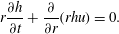 $$\begin{eqnarray}r\frac{\unicode[STIX]{x2202}h}{\unicode[STIX]{x2202}t}+\frac{\unicode[STIX]{x2202}}{\unicode[STIX]{x2202}r}(rhu)=0.\end{eqnarray}$$
Unfortunately, equations (2.4)–(2.6) remain insufficient to derive the thickness profile of the sheet and no obvious boundary condition can be used to make further progress, hence limiting the ability to predict the expansion of the sheet
 $R(t)$
.
2.2 Conflicting sheet thickness profiles proposed in the literature
It is due to this major limitation that conjectures on the thickness profile
 $$\begin{eqnarray}h_{R}(r,t)\sim \frac{t}{r^{3}}\quad \text{and}\quad h_{V}(r,t)\sim \frac{1}{rt},\end{eqnarray}$$
were proposed in the literature. However, no direct measurements of such thickness were reported until the recent experiments of Vernay et al. (Reference Vernay, Ramos and Ligoure2015). The conjecture of Rozhkov et al. (Reference Rozhkov, Prunet-Foch and Vignes-Adler2004) was guided by their experimental observations suggesting that the volume flux
 $q_{s}$
per unit radian in the sheet at a given radial position is constant. Given that
 $$\begin{eqnarray}q_{s}(r,t)=rh(r,t)u(r,t),\end{eqnarray}$$
Rozhkov et al.’s (Reference Rozhkov, Prunet-Foch and Vignes-Adler2004) assumption leads to
 $h\sim t$
. Using
 $h(r,t)=tg(r)$
in (2.6) gives
 $h_{R}(r,t)\sim t/r^{3}$
. The profile of Villermaux & Bossa (Reference Villermaux and Bossa2011) assumes that the spatial thickness profile of an unsteady sheet formed upon drop impact is the same as that of a steady sheet formed from the impact of a continuous jet (Clanet & Villermaux Reference Clanet and Villermaux2002)
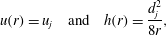 $$\begin{eqnarray}u(r)=u_{j}\quad \text{and}\quad h(r)=\frac{d_{j}^{2}}{8r},\end{eqnarray}$$
where
 $u_{j}$
is the falling jet velocity and
 $d_{j}$
is the diameter of the impacting jet. Thus, the authors sought a time-dependent solution in the form
 $h(r,t)=f(t)/r$
, which combined with (2.6) gives
 $h_{V}(r,t)\sim 1/rt$
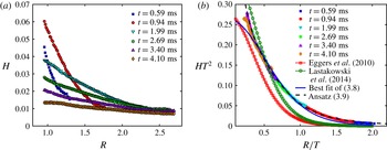
. In sum, the two thickness profiles proposed in the literature differ substantially. However, the findings of Vernay et al. (Reference Vernay, Ramos and Ligoure2015) reproduced in figure 2(a) suggested that both conjectured profiles are partially correct:
 $h_{R}(r,t)$
holds for early times
 $t\ll \unicode[STIX]{x1D70F}=d_{0}/r_{0}$
, while
 $h_{V}(r,t)$
would hold for later times
 $t\gg \unicode[STIX]{x1D70F}$
. It remains difficult to construct the full theory of sheet expansion without more than these limits and no unified profile was proposed to date in the literature for expanding sheets in the air. In § 3, we derive a self-similarity solution that allows us to collapse all the thickness profile data of Vernay et al. (Reference Vernay, Ramos and Ligoure2015) and to develop a unified thickness profile tested and validated by our experiments in §§ 4–7.
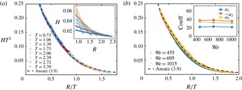
(a) Reproduction of the measurements of sheet thickness reported in Vernay et al. (Reference Vernay, Ramos and Ligoure2015); (b) we collapse the data shown in (a) on a single curve when using the self-similarity solution variables in (3.7) derived in § 3.1 and compare the collapsed data curve with different empirical expressions of similarity solution proposed in the literature and with (3.9) derived in this paper.

3 Unified self-similar thickness profile for an expanding sheet
3.1 Derivation of the self-similar profile of thickness from the equations of motion
In order to derive the general form of
 $h(r,t)$
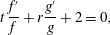
, we return to the equations of motion. Substituting the velocity profile (2.4) into the continuity equation (2.6), we obtain
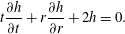 $$\begin{eqnarray}t\frac{\unicode[STIX]{x2202}h}{\unicode[STIX]{x2202}t}+r\frac{\unicode[STIX]{x2202}h}{\unicode[STIX]{x2202}r}+2h=0.\end{eqnarray}$$
Using separation of variables we seek a solution in the form
 $h(r,t)=f(t)g(r)$
, thus,
 $$\begin{eqnarray}t\,\frac{f^{\prime }}{f}+r\frac{g^{\prime }}{g}+2=0,\end{eqnarray}$$
where the prime symbol
 $^{\prime }$
indicates the ordinary derivative of a function with respect to its corresponding variable. Independence of the variables
 $r$
and
 $t$
leads to
 $$\begin{eqnarray}r\frac{g^{\prime }}{g}=a\quad \text{and}\quad t\,\frac{f^{\prime }}{f}=-2-a,\end{eqnarray}$$
where
 $a$
is an arbitrary constant. Hence, our basis of solution is of the form
 $$\begin{eqnarray}f(t)=\frac{1}{t^{2+a}},\quad g(r)=r^{a},\quad \text{and}\quad h(r,t)=f(t)g(r)=\frac{1}{t^{2}}\left(\frac{r}{t}\right)^{a}.\end{eqnarray}$$
The general solution of
 $h(r,t)$
is then in the form
 $$\begin{eqnarray}h(r,t)=\frac{1}{t^{2}}\mathop{\sum }_{m}c_{m}\left(\frac{r}{t}\right)^{m}=\frac{1}{t^{2}}\unicode[STIX]{x1D713}\left(\frac{r}{t}\right).\end{eqnarray}$$
We choose the characteristic length scale to be
 $d_{0}$
and time scale to be
 $\unicode[STIX]{x1D70F}_{0}=d_{0}/u_{0}$
and introduce the dimensionless variables
 $$\begin{eqnarray}R=\frac{r}{d_{0}},\quad H=\frac{h}{d_{0}},\quad \text{and}\quad T=\frac{t}{\unicode[STIX]{x1D70F}}=\frac{u_{0}t}{d_{0}}.\end{eqnarray}$$
We obtain the following dimensionless thickness profile for the expanding sheet in the air:
 $$\begin{eqnarray}H=\frac{1}{T^{2}}F\left(\frac{R}{T}\right)\quad \text{with}\;F\left(\frac{R}{T}\right)=\frac{u_{0}^{2}}{d_{0}^{3}}\unicode[STIX]{x1D713}\left(\frac{r}{t}\right).\end{eqnarray}$$
Such a self-similar profile has not been reported for expanding sheets in the air. In the next section, we assess its ability to collapse prior experimental data. Note that Roisman et al. (Reference Roisman, Berberovi and Tropea2009) arrived at an analogous profile to the one derived here when considering impacts on solid surfaces. There, the authors invoked a derivation in a Lagrangian frame of reference that involved an arbitrary parameter specific to the dynamics of impacts on solid surfaces. Our derivation here differs from that of Roisman et al. (Reference Roisman, Berberovi and Tropea2009).
3.2 Collapse of existing experimental data by the self-similar solution and unified profile
Having obtained a general self-similar profile for the sheet thickness (3.7), we re-plot the experimental data of Vernay et al. (Reference Vernay, Ramos and Ligoure2015) in the new coordinate system
 $Y=HT^{2}$
and
 $X=R/T$
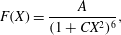
. Figure 2(b) shows the resulting excellent collapse of all their data onto one single master curve. Such collapse shows that the similarity solution (3.7) governs the thickness profile of the sheet expanding in the air. In the context of drop impact and sheet expansion on solid surfaces, Eggers et al. (Reference Eggers, Fontelos, Josserand and Zaleski2010) first proposed an empirical expression for the similarity thickness profile
 $F(X)$
of the sheet in the form
 $$\begin{eqnarray}F(X)=\frac{A}{(1+CX^{2})^{6}},\end{eqnarray}$$
where
 $A=0.27$
and
 $C=0.625$
when fitting the profile with the author’s numerical simulation results. Lastakowski et al. (Reference Lastakowski, Boyer, Biance, Pirat and Ybert2014) verified this empirical expression against experimental data of drop impact on a superheated solid surface where reduced viscous stresses are expected. They found that the fit worked for
 $A=0.40$
and
 $C=0.604$
. However, the expression (3.8) with the coefficients proposed by Eggers et al. (Reference Eggers, Fontelos, Josserand and Zaleski2010) and Lastakowski et al. (Reference Lastakowski, Boyer, Biance, Pirat and Ybert2014) does not capture the thickness profile of the sheet expansion in the air obtained by Vernay et al. (Reference Vernay, Ramos and Ligoure2015) as shown in figure 2(b). Moreover, even when keeping
 $C$
and
 $A$
free, the best fit is not successful in capturing the profile. Thus, another profile is needed. In light of the validity of the profiles
 $h_{R}$
and
 $h_{V}$
in asymptotically large and small times, we propose a new unified analytical functional ansatz
 $F(X)$
for the sheet expansion in the air, with its associated thickness profile
 $H(R,T)$
as
 $$\begin{eqnarray}F(X)=\frac{1}{a_{3}X^{3}+a_{2}X^{2}+a_{1}X}\quad \text{with}\;H(R,T)=\frac{T}{a_{3}R^{3}+a_{2}R^{2}T+a_{1}RT^{2}}.\end{eqnarray}$$
Clearly, for
 $T\ll 1$
,
 $H(R,T)\rightarrow T/R^{3}$
, which is consistent with
 $h_{R}(r,t)$
by Rozhkov et al. (Reference Rozhkov, Prunet-Foch and Vignes-Adler2004) and for
 $T\gg 1$
,
 $H(R,T)\rightarrow 1/RT$
which is consistent with
 $h_{V}(r,t)$
by Villermaux & Bossa (Reference Villermaux and Bossa2011), thus enabling
 $H(R,T)$
(3.9) to unify prior proposed profiles in addition to satisfying the form required for the similarity solution (3.7). As a first validation for this ansatz, we plot the solution using (3.9) in figure 2(b). We find an excellent match of the self-similar solution using
 $F(X)$
(3.9) with the data of Vernay et al. (Reference Vernay, Ramos and Ligoure2015) (figure 2
b). This match was obtained for values of
 $a_{1}=18,a_{2}=-24$
and
 $a_{3}=24$
. Next we evaluate the robustness of (3.9) against our experimental data and provide a range of validity of the self-similar unified solution with respect to surface-to-drop size ratio. We will also discuss and validate the physical meaning of
 $a_{1},a_{2}$
and
 $a_{3}$
in § 7.
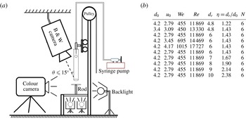
(a) Schematic of the experimental set-up. (b) Table of experimental conditions used: impacting drop diameter
 $d_{0}$
, associated
 $We$
and
 $Re$
, ratio of surface-to-drop size
 $\unicode[STIX]{x1D702}=d_{r}/d_{0}$
, diameter of the solid surface
 $d_{r}$
and number of repeated experiments
 $N$
. Note that for experiments with high Weber number, only 5%–10 % of the drops released led to centred impacts that were kept for the analysis. However, we maintained a uniform sample size of
 $N=6$
impacts per
 $We$
value. The rod was made of stainless steel with equilibrium contact angle of approximately
 $80^{\circ }$
.

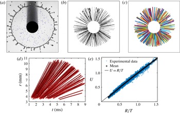
(a) Particle tracers (blue dots) detected in the expanding sheet at a given time. (b) Trajectory formed by the superposition of particle tracers detected at different time. (c) The trajectories captured by our tracking algorithm are shown to collapse well on the real trajectory (time lapse) in (b). (d) Time evolution of the radial position of each particle, showing the conservation of speed along each particle trajectory. (e) Velocity profile of the expanding sheet measured by particle tracers for surface-to-drop size ratio
 $\unicode[STIX]{x1D702}=1.43$
.

4 Direct and indirect measurement of sheet thickness and velocity and validation of the unified sheet thickness profile
We now turn to experiments to assess the robustness of the similarity profile (3.7) and unified functional form (3.9). Figure 3(a) shows a schematic of the set-up. Distilled water (density
 $\unicode[STIX]{x1D70C}=1.0\times 10^{3}~\text{kg}~\text{m}^{-3}$
, surface tension
 $\unicode[STIX]{x1D70E}=72\times 10^{-3}~\text{N}~\text{m}^{-1}$
, viscosity
 $\unicode[STIX]{x1D708}=1.0\times 10^{-6}~\text{m}^{2}~\text{s}^{-1}$
) was used to generate the impacting drops of diameter
 $d_{0}$
. The drop diameters used, and their associated
 $We$
and
 $Re$
, are summarized in figure 3(b).
4.1 Direct measurement of the velocity profile in the expanding sheet in the air
In § 3, we derived the similarity profile (3.7) from the sheet thickness equation assuming a velocity profile
 $u(r,t)=r/t$
in (2.5). We now proceed to verify this profile. In general, two conventional methods are used to measure the fluid velocity field: particle image velocimetry (PIV) (Lastakowski et al.
Reference Lastakowski, Boyer, Biance, Pirat and Ybert2014) and particle tracking velocimetry (PTV). For PIV, a high concentration of microparticles is used. The velocity field is measured by auto- or cross-correlating the intensity distribution of images over small areas at given positions. This is inherently an Eulerian framework. For PTV, particles are tracked individually in a Lagrangian framework. Here, we proceed using PTV given that we expect Lagrangian conservation of velocity according to (2.2), as discussed in § 2.1. We used a small number of particle tracers in the form of polyethylene microspheres of diameter
 ${\approx}50~\unicode[STIX]{x03BC}\text{m}$
and density
 $1.00\pm 0.05~\text{g}~\text{L}^{-1}$
. Figure 4(a) shows a frame captured via high-speed recordings, with the spots in the image showing the particle tracers detected by our image processing algorithm. Superposing the spots for different frames shows the straight lines visualizing the tracer trajectories (figure 4
b). Each line in figure 4(c) indicates a trajectory captured by the tracking algorithm, which collapses very well with the time lapse of the trajectories. The straight line in figure 4(d) shows that each tracer moves in the radial direction at constant speed, as expected from (2.3), thus verifying that (2.2) is indeed governing the dynamics of the sheet for
 $\unicode[STIX]{x1D702}=1.43$
. The intersections of the straight lines with the
 $y$
-axis in figure 4(d) are all close to zero, indicating a back-extrapolated initial position of the parcels at
 $\unicode[STIX]{x1D709}\approx 0$
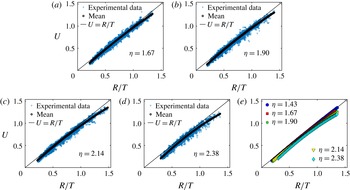
in (2.3). Figure 4(e) shows the good agreement between experimental data and theoretical prediction
 $u=r/t$
.
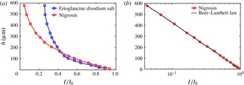
(a) Thickness calibration curve for two different dyes. (b) Calibration curve of Nigrosin following the Beer–Lambert law of absorption.

4.2 Direct measurement of the thickness profile of the expanding sheet in the air
To measure the sheet thickness, we use the light absorption method (Kim & Kim Reference Kim and Kim2005; Vernay et al.
Reference Vernay, Ramos and Ligoure2015). When light passes through a thin film of dyed liquid, it is partially absorbed. The absorption is proportional to the thickness of the film; thus enabling us to measure the thickness. A meticulous calibration is required to obtain an accurate relation between the intensity and the thickness. We use a method of calibration analogous to that used in Vernay et al. (Reference Vernay, Ramos and Ligoure2015). Liquid films of known thicknesses ranging from 10 to 600
 $\unicode[STIX]{x03BC}\text{m}$
were obtained by depositing controlled volumes of dyed liquid between cover slips and imaging through with a uniform high-luminosity backlight. In this study, we used two dyes: Erioglaucine disodium salt diluted in de-ionized water at a concentration of
 $2.5~\text{g}~\text{L}^{-1}$
; and Nigrosin at a concentration of
 $1.2~\text{g}~\text{L}^{-1}$
. Figure 5 shows the intensity–thickness curve for both dyes. The curve of Erioglaucine disodium salt is analogous to that obtained in Vernay et al. (Reference Vernay, Ramos and Ligoure2015, figure 2a therein). However, Nigrosin has a wider range of change of intensity for a given range of thickness and we find that the intensity response of Nigrosin matches perfectly with the Beer–Lambert law of absorption:
 $$\begin{eqnarray}h=\unicode[STIX]{x1D716}\log (I/I_{0}),\end{eqnarray}$$
where
 $I_{0}$
is the incoming background light intensity,
 $I$
is the intensity of the light after passage through the liquid,
 $h$
is the sheet thickness and
 $\unicode[STIX]{x1D716}$
is the fluid absorptivity. Here, we find
 $\unicode[STIX]{x1D716}=185.1~\unicode[STIX]{x03BC}\text{m}$
. The Beer–Lambert law of absorption revealed for Nigrosin is of great interest given that it can provide greater precision in thickness measurements for
 $I/I_{0}\leqslant 0.4$
than Erioglaucine for concentrations of Nigrosin that do not alter the surface tension of the water.
(a) The inset shows the thickness profile
 $H$
as a function of non-dimensional radius
 $R$
at different times of expansion for the impact of a drop of diameter
 $d_{0}=4.2~\text{mm}$
and the impacting velocity
 $u_{0}=2.82~\text{m}~\text{s}^{-1}$
on a rod of diameter
 $d_{r}=6~\text{mm}$
. The time point graphs collapse on a single curve well and follow the similarity profile (3.7). (b) The sheet thickness profiles continue to collapse onto the similarity profile (3.7) for high
 $We$
numbers. The inset shows the value of three coefficients in (3.9), showing the robustness of the functional form and the invariance of the coefficients to changes in
 $We$
. The coefficients are computed from a group of five repeated experiments for each
 $We$
. Note however that each individual experiment follows very well the similarity profile. The small variability in coefficient values over the samples of five repeated experiments is shown in the inset.

Figure 6(a) inset shows the dimensionless thickness profile
 $H$
as a function of non-dimensional radius
 $R$
for a range of times throughout expansion from impact of a drop of diameter
 $d_{0}=4.2~\text{mm}$
on a rod diameter
 $d_{r}=6~\text{mm}$
, corresponding to
 $We=460$
. The graphs collapse on a single curve in the larger figure 6 if re-expressed using the similarity profile (3.7). Moreover, the functional form (3.9) matches very well with the data with coefficient values
 $a_{1}=23.2\pm 1.8$
,
 $a_{2}=-38.4\pm 4.2$
and
 $a_{3}=34.2\pm 1.9$
. We will discuss further the robustness of these values and their physical interpretation in following sections. Here, we also test for the robustness to change in impact
 $We$
. In particular, figure 6(b) shows that the sheet thickness continues to follow (3.7) well when changing impact
 $We$
. We also find that the coefficient values of
 $a_{1}$
,
 $a_{2}$
,
 $a_{3}$
are invariant to the change in
 $We$
as clearly shown in the inset of figure 6(b).
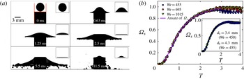
(a) From drop impact to fragmentation of the expanding sheet. The insets show the region in which the fluid is tracked to calculate
 $Q_{s}$
. Scale bar is 3 mm. (b) Time evolution of dimensionless cumulative fluid volume
 $\unicode[STIX]{x1D6FA}_{s}=\hat{\unicode[STIX]{x1D6FA}_{s}}/\unicode[STIX]{x1D6FA}_{0}$
transferred to the expanding sheet for different
 $We$
and impacting drop sizes
 $d_{0}$
(inset). Here,
 $T=t/\unicode[STIX]{x1D70F}$
, with touch-down at
 $T=0$
and
 $\unicode[STIX]{x1D702}=d_{r}/d_{0}=1.43$
.

4.3 Indirect measurement of the thickness profile of the expanding sheet in the air
Apart from the direct measurement of the previous section, we implemented an alternative method of thickness measurement using the cumulative fluid volume
 $\unicode[STIX]{x1D6FA}_{s}$
of the sheet emanating from the rod surface into the air. In theory, the relation between the sheet volume flux per unit radian
 $q_{s}(r,t)$
and the thickness profile
 $h(r,t)$
is derived as (2.8). By introducing the volume flux scale as
 $d_{0}^{2}u_{0}$
, we define the dimensionless volume flux per unit radian to be
 $Q_{s}(R,T)$
. Using (3.9),
 $Q_{s}$
can be expressed as
 $$\begin{eqnarray}Q_{s}(R,T)=\frac{R}{a_{3}R^{2}+a_{2}RT+a_{1}T^{2}}.\end{eqnarray}$$
Non-dimensionalized by the initial drop volume
 $\unicode[STIX]{x1D6FA}_{0}=\unicode[STIX]{x03C0}d_{0}^{3}/6$
, the dimensionless cumulative volume
 $\unicode[STIX]{x1D6FA}_{s}=\hat{\unicode[STIX]{x1D6FA}}_{s}/\unicode[STIX]{x1D6FA}_{0}$
emanating from the rod into the air can be expressed in terms of (3.9) as
 $$\begin{eqnarray}\unicode[STIX]{x1D6FA}_{s}=\int _{T_{0}}^{T}12Q_{s}(R_{d},T)\,\text{d}T=\int _{T_{0}}^{T}\frac{12R_{d}}{a_{3}R_{d}^{2}+a_{2}R_{d}T+a_{1}T^{2}}\,\text{d}T,\end{eqnarray}$$
where
 $T_{0}$
is the dimensionless time when the sheet first reaches the edge of the rod and
 $R_{d}$
is the dimensionless radial position of the surface edge
 $R_{d}=d_{r}/2d_{0}=\unicode[STIX]{x1D702}/2$
.
Experimentally, we developed an image processing method to measure the time evolution of the cumulative volume
 $\unicode[STIX]{x1D6FA}_{s}$
above the rod. Figure 7(a) shows the sequence of events from drop touch down to expansion viewed from the side. The insets in figure 7(a) show examples of processed images used to measure the volume change in the box above the rod, which corresponds to the volume of fluid
 $\hat{\unicode[STIX]{x1D6FA}_{r}}$
remaining on the surface. The cumulative volume
 $\hat{\unicode[STIX]{x1D6FA}_{s}}$
transmitted into the air can then be calculated using
 $\hat{\unicode[STIX]{x1D6FA}_{s}}=\unicode[STIX]{x1D6FA}_{0}-\hat{\unicode[STIX]{x1D6FA}_{r}}$
, in dimensionless form,
 $\unicode[STIX]{x1D6FA}_{s}=1-\unicode[STIX]{x1D6FA}_{r}$
, where
 $\unicode[STIX]{x1D6FA}_{r}=\hat{\unicode[STIX]{x1D6FA}_{r}}/\unicode[STIX]{x1D6FA}_{0}$
.
For a fixed surface-to-drop size ratio
 $\unicode[STIX]{x1D702}=d_{r}/d_{0}$
, we conducted experiments for different Weber numbers (see table in figure 3
b). Figure 7(b) shows the normalized time evolution of the cumulative volume
 $\unicode[STIX]{x1D6FA}_{s}$
for three
 $We$
. The experimental results of
 $\unicode[STIX]{x1D6FA}_{s}$
collapse very well for all
 $We$
considered, thus, the physics governing the sheet profile is independent of
 $We$
for a fixed
 $\unicode[STIX]{x1D702}$
value. This is consistent with the theory in §§ 2 and 3 where surface tension is not involved. We also test for the robustness of the results against changes in drop size
 $d_{0}$
. Figure 7(b) inset confirms the collapse of
 $\unicode[STIX]{x1D6FA}_{s}$
for a given
 $\unicode[STIX]{x1D702}$
. In sum, equation (3.9) is in excellent agreement with our experimental data for a range of
 $We$
and drop sizes. The value of the coefficients obtained for the best match between the experimental data and the ansatz (4.3) is
 $a_{1}=24.4\pm 1.9$
,
 $a_{2}=-38.1\pm 3.5$
and
 $a_{3}=35.2\pm 3.1$
, which is the same as obtained by the direct measurement (§ 4.2) for a surface-to-drop size ratio
 $\unicode[STIX]{x1D702}\approx 1.43$
. In the next section, we evaluate if the match changes with a larger range of surface-to-drop size ratios
 $\unicode[STIX]{x1D702}$
.
5 Effect of surface-to-drop size ratio on sheet dynamics
5.1 Effect of surface-to-drop size ratio on the sheet velocity profile
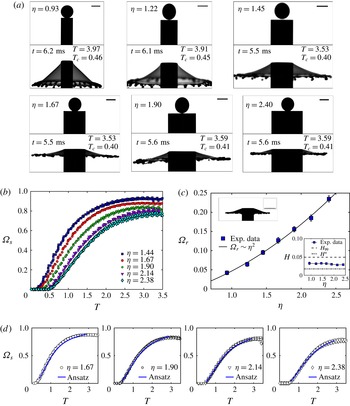
(a) Sheet expansion from impact on surfaces of different surface-to-drop size ratio
 $\unicode[STIX]{x1D702}$
. The lower graph in each panel shows the maximum radial extension of the sheet with
 $T=t/\unicode[STIX]{x1D70F}$
where
 $\unicode[STIX]{x1D70F}$
is the impact time scale,
 $T_{c}=t/\unicode[STIX]{x1D70F}_{c}$
where
 $\unicode[STIX]{x1D70F}_{c}=\sqrt{\unicode[STIX]{x1D70C}\unicode[STIX]{x1D6FA}_{0}/\unicode[STIX]{x03C0}\unicode[STIX]{x1D70E}}$
is the capillary time scale. Scale bar is 3 mm. (b) and (d) Time evolution of the cumulative sheet volume
 $\unicode[STIX]{x1D6FA}_{s}$
for different
 $\unicode[STIX]{x1D702}$
and the corresponding match with (3.9). (c) Dimensionless fluid volume remaining on the surface
 $\unicode[STIX]{x1D6FA}_{s}$
and its corresponding thickness
 $H$
(inset) discussed in § 6.

Having confirmed the independence of the self-similar thickness profile from Weber number and drop size
 $d_{0}$
, we now fix
 $We$
and
 $d_{0}$
and focus on the effect of surface-to-drop size ratio
 $\unicode[STIX]{x1D702}=d_{r}/d_{0}$
(figure 1). Figure 8(a) shows impacts over surfaces with
 $\unicode[STIX]{x1D702}$
values ranging from 0.93 to 2.38 (see table in figure 3
b). There, a clear effect of
 $\unicode[STIX]{x1D702}$
on the angle of the sheet to the horizontal can be noted qualitatively. For the small value of
 $\unicode[STIX]{x1D702}=0.93$
and
 $1.22$
, the drop, upon impact, is deformed by the rod to form an umbrella-shaped sheet, instead of expanding into a horizontal sheet. Figure 8 shows that the vertical displacement of the sheet edge is equivalent to (or even larger than) the horizontal one. Such drop impact is due to the small surface area of the rod compared to the radius of the drop; leading to parts of the drop continuing to fall on the edge of the rod. In other words, the vertical momentum of the drop cannot be fully transferred to horizontal momentum and the sheet cannot be well described by the one-dimensional Euler equation (2.1). Note that this quantitative effect of the surface-to-drop size ratio on the angle of the sheet is investigated outside of the scope of this paper. In addition to the lack of horizontality of the sheet, we cannot use light absorption since the large vertical displacement moves the sheet out of the focus plane required for accurate measurement. For
 $\unicode[STIX]{x1D702}\geqslant 1.43$
, we can however proceed and quantify accurately the effect of increasing
 $\unicode[STIX]{x1D702}$
on both sheet velocity
 $u(r,t)$
and thickness
 $h(r,t)$
profiles as described in § 4.
(a–d) Velocity profile of the expanding sheet measured by particle tracers for different surface-to-drop size ratios
 $\unicode[STIX]{x1D702}$
. (e) Comparison of the velocity profile for all
 $\unicode[STIX]{x1D702}$
values.

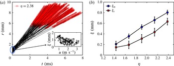
(a) Comparison of the measured position of the particle tracers in the expanding sheet with the theoretical inviscid expected expression (2.3) for the larger surface-to-drop size ratios
 $\unicode[STIX]{x1D702}=2.38$
. Clearly the velocities are constant when the particles are travelling in the expanding sheet in the air (red part of the graph). However, the back-extrapolated origin
 $\unicode[STIX]{x1D709}$
values in (2.3) do not have a clear relation with velocity, showing a breakdown of the inviscid approximation of the velocity field for this larger surface-to-drop size ratio. (b) Experimentally measured
 $\unicode[STIX]{x1D709}$
(mean and standard deviation) values in (2.3) are shown for the full range of surface-to-drop size ratios
 $\unicode[STIX]{x1D702}$
, showing the increasing influence of the history of the fluid on the surface on the velocity profile of the expanding sheet exiting the rod to expand in the air.
 $\unicode[STIX]{x1D709}_{m}$
is the mean value and
 $\unicode[STIX]{x1D709}_{s}$
is the standard deviation of
 $\unicode[STIX]{x1D709}$
for all the particles in one experiment.

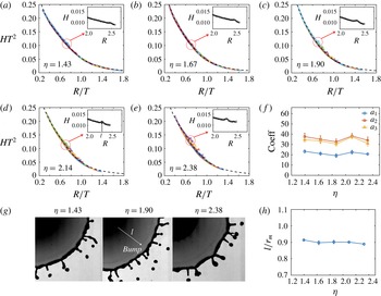
(a–e) Comparison of the direct and indirect measurements of thickness profile and the theoretical similarity thickness profiles for different
 $\unicode[STIX]{x1D702}$
values. The coefficients
 $a_{1},a_{2}$
and
 $a_{3}$
obtained from (3.9) show a relative invariance with
 $\unicode[STIX]{x1D702}$
when correction to the change in the velocity profile, discussed in § 5.1, is applied. The deviation of the measured thickness from a collapsed single curve increases with
 $\unicode[STIX]{x1D702}$
. The circled areas on panels (a–e) are magnified in the insets showing the bump in thickness also shown directly in panel (g). The change in the location of the bump region with
 $\unicode[STIX]{x1D702}$
is quantified in panel (h).

Figure 9(a–e) show the velocity profile obtained by PTV (see § 4.1) for different
 $\unicode[STIX]{x1D702}$
. As
 $\unicode[STIX]{x1D702}$
increases, the measured sheet velocity profile deviates downward from the theoretical prediction (2.4). In other word, the velocity decreases with increasing
 $\unicode[STIX]{x1D702}$
. Note that the tracking of the particles accounted for the angle of the sheet with the horizontal, so the decrease in velocity is not due to an artefact in the tracking. Figure 10(a) shows the time evolution of the radial position of each particle tracer in the expanding sheet for a surface-to-drop size ratio of
 $\unicode[STIX]{x1D702}=2.38$
. This is the Lagrangian representation of the velocity of each tracer in the film. We clearly confirm that once in the air, each tracer moves at a constant speed along its trajectory. The same result is found for all other
 $\unicode[STIX]{x1D702}$
values examined. In other words, the Lagrangian conservation of velocity in the expanding sheet still holds for all
 $\unicode[STIX]{x1D702}$
. However, when leaving the rod, the velocity profile deviates from the inviscid theoretical prediction as the surface-to-drop size ratio
 $\unicode[STIX]{x1D702}$
increases (see figures 9
a–e and 10
a). This is well captured when back extrapolating the initial position of the particles on the rod
 $\unicode[STIX]{x1D709}$
in (2.3) for different
 $\unicode[STIX]{x1D702}$
values. Clearly the values are not zero and increase with
 $\unicode[STIX]{x1D702}$
as shown in figure 10(b).
As discussed in § 2.1, Yarin & Weiss (Reference Yarin and Weiss1995) proposed that the initial position of a fluid particle
 $\unicode[STIX]{x1D709}$
is linearly proportional to its initial velocity, namely,
 $\unicode[STIX]{x1D709}=u/b$
. Figure 10(a) shows the experimental data of
 $\unicode[STIX]{x1D709}$
and
 $u$
from different particle tracers for
 $\unicode[STIX]{x1D702}=2.38$
. No clear relation can be claimed between
 $\unicode[STIX]{x1D709}$
and
 $u$
, which might be due to the sophisticated dynamics of drop impact on surfaces at early times. However, in order to capture the leading-order effect of
 $\unicode[STIX]{x1D702}$
on
 $\unicode[STIX]{x1D709}$
, we take the mean value
 $\unicode[STIX]{x1D709}_{m}$
of
 $\unicode[STIX]{x1D709}$
of all the particle tracers for the same
 $\unicode[STIX]{x1D702}$
. A clear relation of
 $\unicode[STIX]{x1D709}_{m}$
with
 $\unicode[STIX]{x1D702}$
is shown in figure 10(b). The increase of
 $\unicode[STIX]{x1D709}_{m}$
with
 $\unicode[STIX]{x1D702}$
can be explained by the viscous boundary layer, showing the increasing influence of the history of the fluid on the surface on the velocity profile of the expanding sheet exiting the rod to expand in the air. In § 6 we will return to this point to elucidate this effect in the context of the boundary layer formed on the solid surface prior to the fluid expansion in the air.
5.2 Effect of surface-to-drop size ratio on the sheet thickness profile
Figure 11(a–e) show the thickness profile of the sheet obtained by light absorption for different
 $\unicode[STIX]{x1D702}$
. As
 $\unicode[STIX]{x1D702}$
increases, the sheet thickness at different times deviates from a single curve, implying that the similarity solution (3.9) is violated at large
 $\unicode[STIX]{x1D702}$
values. As seen in the previous section, based on PTV, the velocity of the fluid particles in the expanding sheet is
 $u=(r-\unicode[STIX]{x1D709})/t$
, where
 $u$
and
 $\unicode[STIX]{x1D709}$
are the initial conditions of each particle. Although no clear relation is obtained between
 $u$
and
 $\unicode[STIX]{x1D709}$
(figure 10
a inset), the mean value
 $\unicode[STIX]{x1D709}_{m}$
of
 $\unicode[STIX]{x1D709}$
and its standard deviation
 $\unicode[STIX]{x1D709}_{s}$
for all the particles in one video is found to increase with
 $\unicode[STIX]{x1D702}$
(figure 10
b). The increase of
 $\unicode[STIX]{x1D709}_{m}$
indicates that the velocity of fluid particles decreases further away from its theoretical expected value. The increase of
 $\unicode[STIX]{x1D709}_{s}$
indicates the unpredictability of the initial velocity of the fluid particles within the sheet, reflecting that the very early dynamics cannot be expressed explicitly with a similarity solution, particularly as
 $\unicode[STIX]{x1D702}$
increases. Indeed, we find that as
 $\unicode[STIX]{x1D702}$
increases, the measured thickness profile has an increasingly poor collapse onto a single curve, as shown in figure 11(a–e).
However, although the measured sheet thickness does not strictly collapse on a single curve for larger
 $\unicode[STIX]{x1D702}$
, the ansatz (3.9) can still, to a large extent, match with the experimental data, and describe the evolution of the sheet thickness profile once the correction in velocity profile is included. We compared the coefficients in (3.9) from best match for different
 $\unicode[STIX]{x1D702}$
values and found that the three coefficients also remain constant with
 $\unicode[STIX]{x1D702}$
as shown in figure 11(g). The standard deviation of each coefficient for the same
 $\unicode[STIX]{x1D702}$
is equivalent to the derivation of its mean between different
 $\unicode[STIX]{x1D702}$
, indicating that the effect of the surface-to-drop size ratio
 $\unicode[STIX]{x1D702}$
on the thickness is not dominant per say, but mostly eroding the self-similarity of the velocity filed itself.
To verify further this result, we compare the direct and indirect measurements using the cumulative volume
 $\unicode[STIX]{x1D6FA}_{s}$
of the fluid emanating from the rod. Figure 8(b) and (d) show the time evolution of
 $\unicode[STIX]{x1D6FA}_{s}$
for different
 $\unicode[STIX]{x1D702}$
values. The different delays in onset of
 $\unicode[STIX]{x1D6FA}_{s}$
growth reflect the different travel times for the fluid to reach the edge of the rod. The experimental results show that the volume growth rate of
 $\unicode[STIX]{x1D6FA}_{s}$
decreases with
 $\unicode[STIX]{x1D702}$
, which is in agreement with the data of sheet velocity decrease with
 $\unicode[STIX]{x1D702}$
. As
 $\unicode[STIX]{x1D702}$
increases, the velocity profile can be approximately expressed by
 $u=(r-\unicode[STIX]{x1D709}_{m})/t$
, while the thickness profile
 $h(r,t)$
, though not collapsing strictly on a curve, still can be described by ansatz (3.9) with mostly invariant coefficients. Using (2.8) and (3.9), the cumulative volume
 $\unicode[STIX]{x1D6FA}_{s}$
for large
 $\unicode[STIX]{x1D702}$
can be modified to read
 $$\begin{eqnarray}\unicode[STIX]{x1D6FA}_{s}^{\prime }=\int _{T_{0}}^{T}\frac{12(R_{d}-\unicode[STIX]{x1D709}_{m})}{a_{3}R_{d}^{2}+a_{2}R_{d}T+a_{1}T^{2}}\,\text{d}T.\end{eqnarray}$$
Using the values of
 $\unicode[STIX]{x1D709}_{m}$
from figure 10(a) and the three coefficients
 $a_{1}$
,
 $a_{2}$
,
 $a_{3}$
from figure 11(f), the time evolution of
 $\unicode[STIX]{x1D6FA}_{s}$
is estimated using (5.1). Figure 8(d) shows that the time evolution of
 $\unicode[STIX]{x1D6FA}_{s}$
matches well with the experimental data for all different
 $\unicode[STIX]{x1D702}$
after this correction is applied. This result shows that the decrease in the growth rate of the volume
 $\unicode[STIX]{x1D6FA}_{s}$
with
 $\unicode[STIX]{x1D702}$
is primarily driven by the lower velocity of the fluid reaching the edge of the larger rods.
Another interesting phenomenon discovered during the experimental analysis is that a ‘bump’ (local thick region) exists around the outer edge of the unsteady expanding sheet (preceding the rim position). The bump can be directly observed from the snapshots shown in figure 11(g) when the sheet reaches its maximum radial extension, where a lighter region appears. We performed a preliminary quantification of this transition region and measured its radial position
 $l$
from the rod edge
 $r_{d}$
at the time of maximum sheet extension. Figure 11(h) shows this position
 $l$
normalized by the maximum sheet radius
 $r_{m}$
for different
 $\unicode[STIX]{x1D702}$
. The bump is located at approximately 90 % of the total sheet radius. For large
 $\unicode[STIX]{x1D702}$
, the region between the ‘bump’ and the rim surrounding the sheet is where we observe large deviation between the measured sheet thickness and similarity profile. This region is also circled in figures 11(a–e). A more detailed study of this bump is out of the scope of the present study, and will be a subject of future work.
6 Surface viscous boundary layer and energy dissipation
In the present section we will rationalize the values of
 $\unicode[STIX]{x1D709}$
discussed in § 5.1 by examining the effect of dissipation on the surface via boundary layer formation. We start by verifying that the thickness of the minimum volume of fluid remaining on the rod surface is compatible with a simple model of the boundary layer on the surface. Figure 8(b) shows the time evolution of the sheet cumulative volume
 $\unicode[STIX]{x1D6FA}_{s}$
for
 $\unicode[STIX]{x1D702}\geqslant 1$
obtained from analysis of the crushing volume above the surfaces used, such as those shown in figure 8(a). The
 $\unicode[STIX]{x1D6FA}_{s}$
curves all grow and saturate below
 $\unicode[STIX]{x1D6FA}_{s}=1$
. This upper bound supports the accuracy of our image processing and method by satisfying conservation of volume
 $\unicode[STIX]{x1D6FA}_{s}<\unicode[STIX]{x1D6FA}_{0}$
. The
 $\unicode[STIX]{x1D6FA}_{s}$
curves reach different saturation levels (figure 8
b), reflecting that different fluid volumes remain on the surface for different
 $\unicode[STIX]{x1D702}$
values as shown in figure 8(c). In fact, the residual volume
 $\unicode[STIX]{x1D6FA}_{r}$
on the surface increases with
 $\unicode[STIX]{x1D702}$
. We measure
 $\unicode[STIX]{x1D6FA}_{r}$
when the sheet in the air reaches its maximum extension to ensure minimal effect of fluid retraction from capillary forces and directly quantify the volume
 $\unicode[STIX]{x1D6FA}_{r}$
of fluid remaining on the surfaces. Figure 8(c) inset shows that the average fluid layer thickness on the surfaces is constant for all surface-to-drop size ratios
 $\unicode[STIX]{x1D702}$
. Thus,
 $\unicode[STIX]{x1D6FA}_{r}$
is expected to be proportional to the area of the surface
 $d_{r}^{2}\sim \unicode[STIX]{x1D702}^{2}$
, which is confirmed in figure 8(c).
We now show that this thickness is in fact governed by the viscous boundary layer. By analogy with the Blasius flat-plate profile for a steady radially expanding flow (Watson Reference Watson1964), the thickness of the boundary layer, defined at the distance at which the inner velocity is equal to 99 % of the external imposed velocity, is
 $\unicode[STIX]{x1D6FF}_{99}=2.85\sqrt{\unicode[STIX]{x1D708}r/U}$
. The displacement thickness, defined as the distance over which the outer flow streamlines are displaced due to the boundary layer, is
 $\unicode[STIX]{x1D6FF}^{\ast }=\int _{0}^{\infty }(1-u/U)\,\text{d}y=0.99\sqrt{\unicode[STIX]{x1D708}r/U}$
, where
 $U$
is the velocity of the external flow, which, in our case, is given by (2.4),
 $U=r/t$
, thus,
 $$\begin{eqnarray}\unicode[STIX]{x1D6FF}_{99}=2.85\sqrt{\unicode[STIX]{x1D708}t}\quad \text{and}\quad \unicode[STIX]{x1D6FF}^{\ast }=0.99\sqrt{\unicode[STIX]{x1D708}t}.\end{eqnarray}$$
For water,
 $\unicode[STIX]{x1D708}=1.0\times 10^{-6}~(\text{m}^{2}~\text{s}^{-1})$
, the sheet reaches its maximum radius at time
 $T\approx 5.5$
ms (figure 8
a) at which point the boundary layer thicknesses are
 $\unicode[STIX]{x1D6FF}_{99}=0.213~\text{mm}$
and
 $\unicode[STIX]{x1D6FF}^{\ast }=0.074~\text{mm}$
, corresponding to dimensionless thicknesses
 $H_{99}=\unicode[STIX]{x1D6FF}_{99}/d_{0}=0.0496$
and
 $H^{\ast }=0.0173$
, respectively. Figure 8(c) inset shows that our experimentally measured residual fluid thickness on the surfaces is independent of
 $\unicode[STIX]{x1D702}$
and is consistent with (6.1a,b
) with values of the same order of magnitude and between
 $H_{99}$
and
 $H^{\ast }$
, and is captured in the form of (6.1a,b
) by
 $$\begin{eqnarray}\unicode[STIX]{x1D6FF}_{\text{exp}}=1.85\sqrt{\unicode[STIX]{x1D708}t}.\end{eqnarray}$$
After confirming the existence of the viscous boundary layer and that a Blasius-type model captures well our data, we now estimate the viscous dissipation induced by such a layer. In theory, the rate of viscous dissipation can be expressed as
 $$\begin{eqnarray}D=\int _{V}2\unicode[STIX]{x1D707}\unicode[STIX]{x1D626}_{ij}\unicode[STIX]{x1D626}_{ij}\text{d}V\quad \text{with}\;\unicode[STIX]{x1D626}_{ij}=\frac{1}{2}\left(\frac{\unicode[STIX]{x2202}u_{j}}{\unicode[STIX]{x2202}x_{i}}+\frac{\unicode[STIX]{x2202}u_{i}}{\unicode[STIX]{x2202}x_{j}}\right),\end{eqnarray}$$
where
 $u_{i}$
is the component of velocity in direction
 $i$
and
 $\unicode[STIX]{x1D626}_{ij}$
is the
 $i,j$
component of strain rate tensor. In our problem. the expanding sheet is mostly radial, namely
 $\boldsymbol{u}=u\boldsymbol{e}_{\mathit{r}}$
. Within the boundary layer,
 $u=u(r,z,t)$
, where
 $z$
is the vertical coordinate value. Scaling analysis using drop size
 $d_{0}$
and velocity
 $u_{0}$
gives the scaling of the thickness of the boundary layer as
 $\unicode[STIX]{x1D6FF}\sim \sqrt{\unicode[STIX]{x1D708}\unicode[STIX]{x1D70F}}$
, where
 $\unicode[STIX]{x1D70F}=d_{0}/u_{0}$
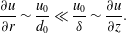
is the time scale. For a water drop with initial conditions listed in figure 3(b),
 $\unicode[STIX]{x1D6FF}\ll d_{0}$
, thus,
 $$\begin{eqnarray}\frac{\unicode[STIX]{x2202}u}{\unicode[STIX]{x2202}r}\sim \frac{u_{0}}{d_{0}}\ll \frac{u_{0}}{\unicode[STIX]{x1D6FF}}\sim \frac{\unicode[STIX]{x2202}u}{\unicode[STIX]{x2202}z}.\end{eqnarray}$$
The rate of dissipation within the boundary layer can then be simplified to
 $$\begin{eqnarray}D(t)\approx \int _{V}\unicode[STIX]{x1D707}\left(\frac{\unicode[STIX]{x2202}u}{\unicode[STIX]{x2202}z}\right)^{2}\,\text{d}V\approx \int _{0}^{r_{e}}\unicode[STIX]{x1D707}\left(\frac{r}{t\unicode[STIX]{x1D6FF}_{0}}\right)^{2}2\unicode[STIX]{x03C0}r\unicode[STIX]{x1D6FF}_{0}\,\text{d}r,\end{eqnarray}$$
where
 $\unicode[STIX]{x1D6FF}_{0}$
is the characteristic boundary layer thickness. Here, from the experimental result (6.2), we choose
 $\unicode[STIX]{x1D6FF}_{0}=\unicode[STIX]{x1D6FF}_{\text{exp}}=1.85\sqrt{\unicode[STIX]{x1D708}t}$
.
 $r_{e}$
is the radius of the rod
 $r_{d}$
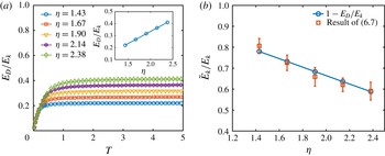
when the expanding sheet extends beyond the edge of the rod and is otherwise the radius of the sheet. Figure 12(a) shows the time evolution of the dissipation
 $E_{D}$
due to the boundary layer for different
 $\unicode[STIX]{x1D702}$
values, which is estimated by
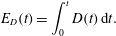 $$\begin{eqnarray}E_{D}(t)=\int _{0}^{t}D(t)\,\text{d}t.\end{eqnarray}$$
The dissipation
 $E_{D}$
is non-dimensionalized by the initial kinetic energy of the falling drop
 $E_{k}=\unicode[STIX]{x1D70C}\unicode[STIX]{x1D6FA}_{0}u_{0}^{2}/2$
. Since the external velocity profile
 $u=r/t$
is inversely proportional to time, we expect the total dissipation to reach a limiting value.
(a) Time evolution of the theoretically estimated viscous dissipation on the rod for different
 $\unicode[STIX]{x1D702}$
. The dissipation
 $E_{D}$
is non-dimensionalized by the initial kinetic energy of the falling drop
 $E_{k}$
. The inset shows the limit value of
 $E_{D}$
for different
 $\unicode[STIX]{x1D702}$
. (b) Experimental measurement of the total kinetic energy
 $\tilde{E}_{k}^{d}$
of the fluid emanating from the edge of the rod for different
 $\unicode[STIX]{x1D702}$
, non-dimensionalized by
 $E_{k}$
. The data are in good agreement with the prediction based on the boundary layer discussed in § 6.

We expect the energy loss due to viscous dissipation to decrease the velocity of the fluid elements leaving the rod surface and, in fact, this is what we observed and discussed in § 5.1. In theory, the velocity of the fluid particle at the edge of the rod is given by (2.5)
 $u_{d}=r_{d}/t$
, where
 $r_{d}$
is the radius of the rod. However, we measured
 $\tilde{u} _{d}=(r_{d}-\unicode[STIX]{x1D709}_{m})/t$
, where
 $\unicode[STIX]{x1D709}_{m}$
is the mean value of the back-extrapolated initial position of the particle tracers discussed in § 5.1. Since the relations between
 $\unicode[STIX]{x1D709}_{m}$
and
 $\unicode[STIX]{x1D702}$
are shown in figure 10(b), the cumulative kinetic energy of the fluid passing through the edge of the rod up to a time
 $t$
can be estimated as
 $$\begin{eqnarray}E_{k}^{d}(t)=\int _{0}^{t}\frac{1}{2}\unicode[STIX]{x1D70C}\cdot 2\unicode[STIX]{x03C0}q(r_{d},t)u(r_{d},t)^{2}\,\text{d}t=\int _{0}^{t}\unicode[STIX]{x1D70C}\unicode[STIX]{x03C0}r_{d}h(r_{d},t)u(r_{d},t)^{3}\,\text{d}t.\end{eqnarray}$$
Based on energy conservation in absence of viscosity (
 $u_{d}=r_{d}/t$
), we have
 $E_{k}^{d}(\infty )=E_{k}$
, where
 $E_{k}=\unicode[STIX]{x1D70C}\unicode[STIX]{x1D6FA}_{0}u_{0}^{2}/2$
is the initial kinetic energy of the falling drop. As discussed in § 5, the rod size and associated viscous effect is mostly limited to changing the velocity rather than the sheet thickness profile. Thus, correcting for this effect as was done in (5.1), the experimental value of
 $\tilde{E}_{d}^{k}/E_{k}$
can be simplified as
 $$\begin{eqnarray}\frac{\tilde{E}_{k}^{d}(\infty )}{E_{k}}=\frac{\tilde{E}_{k}^{d}(\infty )}{E_{k}^{d}(\infty )}\approx \left(\frac{r_{d}-\unicode[STIX]{x1D709}_{m}}{r_{d}}\right)^{3}.\end{eqnarray}$$
Figure 12(b) shows the experimental measurement of
 $E_{k}^{d}/E_{k}$
with increasing
 $\unicode[STIX]{x1D702}$
. The direct measurement is in good agreement with the theoretical prediction
 $1-E_{D}(\infty )/E_{k}$
for different
 $\unicode[STIX]{x1D702}$
, where
 $E_{D}(\infty )$
is the total dissipation shown in figure 12(a) inset. This verifies that the decrease of the velocity field
 $u(r,t)=(r-\unicode[STIX]{x1D709}_{m})/t$
for large
 $\unicode[STIX]{x1D702}$
is well captured by our proposed Blasius-type boundary layer dissipation on the surface preceding the flow over the edge of the rod.
7 Physical meaning of ansatz
 $F(X)$
and associated values of
$a_{1},a_{2}$
and
$a_{3}$


We now return to the proposed ansatz (3.9) to rationalize its form and the physical meaning of its coefficients. We focus herein on the ideal case of
 $\unicode[STIX]{x1D702}=1.43$
where the sheet expands horizontally and the viscous effects of the rod are minimal. For this configuration
 $u=r/t$
remains true in the sheet (figure 4
e). Thus, the similarity profile (3.5) can be strictly derived from continuity (2.6). Based on our prior analysis, the fluid dynamics in the air is well captured by the Euler equation and the continuity equation. The dynamics of the crushing drop on the surface would provide the missing boundary and initial conditions to this problem. However, the crushing dynamics on the rod is a priori too complex and remains an open problem. Two recent studies examined the very early dynamics of tip of lamella formation at impact (Thoroddsen, Takehara & Etoh Reference Thoroddsen, Takehara and Etoh2012; Riboux & Gordillo Reference Riboux and Gordillo2014) when the contact is a very small fraction of the drop radius. However, a time gap remains between such early dynamics (
 $T\sim O(0.1)$
) and what we mean in the present study by ‘early’ dynamics (
 $O(0.1)\ll T\ll O(1)$
). Namely, we assume that a sheet has already emerged throughout the reminder of our discussion. Starting from this simple assumption, we now attempt to simplify the physical picture to connect the early dynamics of drop deformation on the surface to the subsequent change in its sheet thickness profile in the air. Next, we show that our simplified proposed model of the crushing drop allows to rationalize the physical interpretation of the coefficients
 $a_{1},a_{2}$
and
 $a_{3}$
in (3.9).
7.1 Early dynamics of crushing: infinite source condition prescribing
$a_{3}$

The effect of the crushing dynamics on the sheet expansion in the air can be modelled as a boundary condition to the sheet expanding in the air. For example, the evolution of the sheet thickness at the edge of the rod
 $h_{d}(t)=h(r_{d},t)$
or
 $H_{d}(T)=\unicode[STIX]{x1D6F9}(T)$
in non-dimensional form. Here,
 $\unicode[STIX]{x1D6F9}(T)$
is an arbitrary function only varying with time. Its form is prescribed by the crushing dynamics occurring on the rod. Using the similarity profile (3.5), (2.8) and
 $H_{d}(T)=H(R_{d},T)$
, the full temporal and spatial profile of the sheet thickness
 $H(R,T)$
can be related to
 $\unicode[STIX]{x1D6F9}(T)$
by
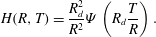 $$\begin{eqnarray}H(R,T)=\frac{R_{d}^{2}}{R^{2}}\unicode[STIX]{x1D6F9}\left(R_{d}\frac{T}{R}\right).\end{eqnarray}$$
Recall that in § 4 we already verified that the coefficients determined by the direct measurement of the sheet thickness are equal to those determined by the cumulative volume leaving the rod
 $\unicode[STIX]{x1D6FA}$
for
 $\unicode[STIX]{x1D702}$
values low enough to neglect viscous effects. This match is another confirmation that the boundary condition at the edge is critical in shaping the subsequent thickness evolution of the expanding sheet in the air.
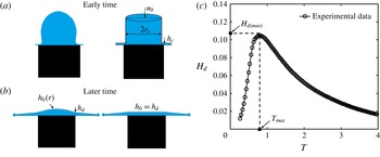
(a) Schematic of drop geometry on the rod surface at early time and (b) at late time. (c) Experimental data of the time evolution of the sheet thickness at the edge of the rod for
 $\unicode[STIX]{x1D702}=1.43$
.

Therefore, the key to rationalizing the expression of ansatz (3.9) for the sheet thickness profile is to understand its boundary condition. Figure 13(a) shows the schematic diagram of the drop impact phenomenon at the early time
 $t\ll \unicode[STIX]{x1D70F}=d_{0}/u_{0}$
. At early times, the expanding sheet is growing at the bottom of the drop (as well documented in prior work such as Thoroddsen et al.
Reference Thoroddsen, Takehara and Etoh2012) and the sheet volume is much smaller than that of the deforming drop. In this limit, we assume that the drop behaves like an infinite source supporting the growth of the sheet. In addition, at this early time, the drop had just touched the rod surface, thus, we also assume that the velocity of the fluid remains uniformly
 $u_{0}$
. Simplifying this geometry, we consider a cylindrical shape with radius
 $r_{c}$
of same total volume as that of the original drop and with the same height as that of the drop, leading to
 $r_{c}=\sqrt{2/3}r_{0}$
. Choosing a control volume around the cylinder, volume conservation provides the evolution of the sheet thickness
 $h_{c}(t)=h(r_{c},t)$
as
 $$\begin{eqnarray}2\unicode[STIX]{x03C0}r_{c}u(r_{c},t)h_{c}(t)=\unicode[STIX]{x03C0}r_{c}^{2}u_{0}\quad \Longrightarrow \quad h_{c}(t)=\frac{u_{0}t}{2}~\text{or}~H_{c}(T)=T/2,\end{eqnarray}$$
where
 $u(r_{c},t)=r_{c}/t$
and
 $H_{c}=h_{c}/d_{0}$
. Using the boundary conditions (7.2), (3.6a–c
) and (7.1), and
 $R_{c}=r_{c}/d_{0}$
, the thickness profile of the entire sheet can be expressed in dimensionless form as
 $$\begin{eqnarray}H(R,T)=\frac{R_{c}^{2}}{R^{2}}H_{c}\left(R_{c}\frac{T}{R}\right)=\frac{R_{c}^{3}T}{2R^{3}},\end{eqnarray}$$
which is analogous to the profile proposed by Rozhkov et al. (Reference Rozhkov, Prunet-Foch and Vignes-Adler2002) or the early time limit of (3.9) with
 $\lim _{T\rightarrow 0}H(R,T)=T/a_{3}R^{3}$
; thus,
 $a_{3}=2/R_{c}^{3}$
.
7.2 Advanced time dynamics of crushing: boundary conditions at the edge of the rod prescribing
$a_{1}$
and
$a_{2}$


As time advances, the finite volume of the drop starts to matter. The drop can no longer provide constant mass flux to the sheet. At this later time
 $t\gg \unicode[STIX]{x1D70F}$
, the shape of the drop is deformed to have a smooth connection with the expansion sheet, as illustrated in our schematic figure 13(b). Here, choosing the control volume with its boundary at the edge of the rod, volume conservation leads to
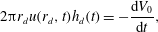 $$\begin{eqnarray}2\unicode[STIX]{x03C0}r_{d}u(r_{d},t)h_{d}(t)=-\frac{\text{d}V_{0}}{\text{d}t},\end{eqnarray}$$
where
 $V_{0}$
is the volume of the fluid on the rod. Assuming that the height of the fluid on the rod is
 $h_{0}(r,t)$
(see figure 13
b), the mean fluid thickness on the rod is
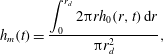 $$\begin{eqnarray}h_{m}(t)=\frac{\displaystyle \int _{0}^{r_{d}}2\unicode[STIX]{x03C0}rh_{0}(r,t)\,\text{d}r}{\unicode[STIX]{x03C0}r_{d}^{2}},\end{eqnarray}$$
and we can simplify (7.4) to
 $$\begin{eqnarray}2\frac{h_{d}(t)}{t}=-\frac{\text{d}h_{m}}{\text{d}t}.\end{eqnarray}$$
At this later time dynamics, fluid continues to be transferred from the drop to the sheet, and so we expect that
 $h_{m}(t)$
and
 $h_{d}(t)$
both decrease with time. We now go further and assume that
 $h_{m}$
and
 $h_{d}$
are proportional to each other with
 $h_{m}(t)=ch_{d}(t)$
. Using this assumption, the solution to (7.6) is reduced to
 $$\begin{eqnarray}h_{d}\sim \frac{1}{t^{2/c}}.\end{eqnarray}$$
In the extreme (or large time) case of a flat fluid surface on the rod (see figure 13
b) we have
 $h_{d}=h_{m}=h_{0}$
, thus
 $c=1$
and
 $h_{d}(t)\sim 1/t^{2}$
. Combining (7.1) and (3.6a–c
), the dimensionless thickness profile of the entire sheet then becomes
 $$\begin{eqnarray}H(R,T)\sim \frac{1}{T^{2}},\end{eqnarray}$$
which is a profile proposed by Yarin & Weiss (Reference Yarin and Weiss1995) in the context of drop impacts on solid surfaces. Physically, when the volume of fluid on the rod approaches zero, the thickness
 $h_{d}$
of the sheet at
 $r_{d}$
can be considered equal to the mean thickness
 $h_{m}$
on the rod. Although promising, our experimental results and those of Vernay et al. (Reference Vernay, Ramos and Ligoure2015) do not support this physical picture. In fact, we reported a sheet thickness at late times
 $t\gg \unicode[STIX]{x1D70F}$
approaching
 $1/T$
, rather than
 $1/T^{2}$
. Within our range of assumptions above, this would suggest that
 $h_{m}=h_{0}$
is never reached during sheet expansion. Instead, our experiments support a late time
 $h_{d}(t)=1/t$
, leading to
 $c=2$
. In this case, using (7.1), the full sheet thickness profile is
 $$\begin{eqnarray}H(R,T)\sim \frac{1}{RT}.\end{eqnarray}$$
Villermaux & Bossa (Reference Villermaux and Bossa2011) proposed this profile based on the assumption that the spatial profile of the sheet would be equal to that of the steady-state sheet profile formed by the impact of a continuous liquid jet on a small surface. Next, we propose a complementary physical interpretation related to the drop geometry on the surface.
We have already discussed that within the framework of our physical representation of drop crushing at later times (figure 13
b), the sheet thickness at the edge of the rod is
 $1/t^{2/c}$
and our experiments give
 $c=2$
. This implies that the mean thickness
 $h_{m}$
of fluid on the rod is approximately twice that of the sheet
 $h_{d}$
at the edge of the rod, hence, relating the functional form to a simplified drop geometry on the rod. Recall that at the edge of the rod
 $R_{d}$
, the non-dimensional sheet thickness
 $H_{d}(T)\sim T$
increases with time when
 $T\ll 1$
, while
 $H_{d}(T)\sim 1/T$
decreases with time when
 $T\gg 1$
. Such non-monotonic evolution of
 $H_{d}(T)$
is described well by
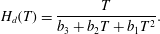 $$\begin{eqnarray}H_{d}(T)=\frac{T}{b_{3}+b_{2}T+b_{1}T^{2}}.\end{eqnarray}$$
Combining (7.10) and (7.1), we re-express the ansatz (3.9) with coefficients
 $a_{3}=b_{3}/R_{d}^{3}$
,
 $a_{2}=b_{2}/R_{d}^{2}$
and
 $a_{1}=b_{1}/R_{d}$
. We already determined that
 $a_{3}$
is governed by (7.2) in § 7.1. We now show how
 $a_{2}$
and
 $a_{1}$
can be prescribed by the physics of the sheet formation at the edge of the rod.
Given that
 $H_{d}(T)$
first increases and then decreases, it has one maximum
 $H_{d}(max)$
at a time
 $T_{max}$
, which can be determined by equating to zero the derivative of (7.10):
 $$\begin{eqnarray}H_{d(max)}=1/(2\sqrt{b_{1}b_{3}}+b2)\quad \text{when}\;T_{max}=\sqrt{b_{3}/b_{1}}.\end{eqnarray}$$
Consider
 $$\begin{eqnarray}\unicode[STIX]{x1D6FD}_{1}=\sqrt{b_{3}/b_{1}}=T_{max},\quad \unicode[STIX]{x1D6FD}_{2}=2\sqrt{b_{1}b_{3}}+b2=\frac{1}{H_{d(max)}},\quad \unicode[STIX]{x1D6FD}_{3}=b_{3},\end{eqnarray}$$
used to re-arrange (7.10) into
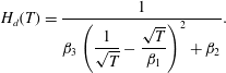 $$\begin{eqnarray}H_{d}(T)=\frac{1}{\displaystyle \unicode[STIX]{x1D6FD}_{3}\left(\frac{1}{\sqrt{T}}-\frac{\sqrt{T}}{\unicode[STIX]{x1D6FD}_{1}}\right)^{2}+\unicode[STIX]{x1D6FD}_{2}}.\end{eqnarray}$$
Using (7.1), the ansatz (3.9) can also be re-written as
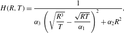 $$\begin{eqnarray}H(R,T)=\frac{1}{\displaystyle \unicode[STIX]{x1D6FC}_{3}\left(\sqrt{\frac{R^{3}}{T}}-\frac{\sqrt{RT}}{\unicode[STIX]{x1D6FC}_{1}}\right)^{2}+\unicode[STIX]{x1D6FC}_{2}R^{2}},\end{eqnarray}$$
with
 $$\begin{eqnarray}\unicode[STIX]{x1D6FC}_{1}=\frac{\unicode[STIX]{x1D6FD}_{1}}{R_{d}}=\frac{T_{max}}{R_{d}},\quad \unicode[STIX]{x1D6FC}_{2}=\frac{\unicode[STIX]{x1D6FD}_{2}}{R_{d}^{2}}=\frac{1}{H_{d(max)}R_{d}^{2}},\quad \unicode[STIX]{x1D6FC}_{3}=\frac{\unicode[STIX]{x1D6FD}_{3}}{R_{d}^{3}},\end{eqnarray}$$
and the relation with
 $a_{1}$
,
 $a_{2}$
and
 $a_{3}$
is then
 $$\begin{eqnarray}\unicode[STIX]{x1D6FC}_{1}=\sqrt{\frac{a_{3}}{a_{1}}},\quad \unicode[STIX]{x1D6FC}_{2}=2\sqrt{a_{1}a_{3}}+a_{2},\quad \unicode[STIX]{x1D6FC}_{3}=a_{3}.\end{eqnarray}$$
Therefore,
 $\unicode[STIX]{x1D6FC}_{3}=a_{3}$
remains prescribed by the early time dynamics of (7.2) in § 7.1, while
 $\unicode[STIX]{x1D6FC}_{2}$
and
 $\unicode[STIX]{x1D6FC}_{3}$
are directly related to the maximum sheet thickness
 $H_{d(max)}$
at the edge of the rod
 $R_{d}$
reached at time
 $T_{max}$
.
7.3 Direct verification of the physical interpretation of
$a_{1}$
,
$a_{2}$
and
$a_{3}$


Concerning
 $a_{3}$
, we established herein and in § 7.1 that
 $\unicode[STIX]{x1D6FC}_{3}=a_{3}=2/R_{c}^{3}=29.4$
, which is close to the experimental value we obtained to be
 $a_{3}=34.3$
from the match between direct and indirect thickness measurements in § 4 and the functional form (3.9) for
 $\unicode[STIX]{x1D702}=1.43$
. This match supports that at the early time of impact (
 $t\ll t_{c}$
), a constant mass flux
 $q_{0}=\unicode[STIX]{x03C0}r_{c}^{2}u_{0}$
is transferred from the drop into the sheet at
 $r=r_{c}$
and provides a simple geometrical representation of this regime (illustration in figure 13
a).
Concerning
 $a_{1}$
and
 $a_{2}$
, it is more difficult to derive exactly
 $T_{max}$
and
 $H_{d(max)}$
from theory given the need for a full and detailed estimation of drop deformation during crushing, which remains an open problem. However, we can still go further and examine the validity of our proposed physical analogy directly using our experimental results. Our experiments allow us to measure directly
 $T_{max}$
and
 $H_{d(max)}$
at the edge of the rod (e.g. from side view). For
 $\unicode[STIX]{x1D702}=1.43$
, we find
 $T_{max}=0.86$
and
 $H_{d(max)}=0.106$
(see figure 13
b). Using (7.16a–c
), these values lead to
 $\unicode[STIX]{x1D6FC}_{1}=1.20$
and
 $\unicode[STIX]{x1D6FC}_{2}=18.2$
. By comparison, the values obtained in § 5 from the match between the measurement of thickness of the entire sheet in the air and ansatz (3.9) are
 $\unicode[STIX]{x1D6FC}_{1}=1.21$
and
 $\unicode[STIX]{x1D6FC}_{2}=17.8$
. These values are in excellent agreement with the values obtained from the boundary condition at the edge of the rod via
 $T_{max}$
and
 $H_{d(max)}$
. In summary, the match of values for
 $a_{1}$
,
 $a_{2}$
and
 $a_{3}$
between prediction and experiments supports our proposed physical interpretation of the coefficients in (3.9) and provide a way to connect the crushing dynamics of the drop on the surface to the expanding sheet in the air via a simplified physical picture of the process spanning early to late times.
8 Conclusion
In conclusion, we have studied the expanding sheet formed upon impact of a drop on a surface of comparable size to that of the drop. We derived a unified self-similar solution for the unsteady inviscid radial thickness profile of the expanding sheet from first principles. This profile allows to collapse on a single curve the direct measurements of sheet thickness profile for impacts on targets reported in the literature and those conducted in this study. We also directly measured and verified the thickness and velocity profiles of the expanding sheet in the air for a range of surface-to-drop size ratios and compared them to the inviscid profiles expected from inviscid theory. We proposed and validated a unified functional form (3.9) governing the unsteady inviscid sheet thickness profile which connects and reconciles the two conflicting thickness profiles proposed in the literature thus far. We showed that such a profile is independent of the change of Weber number and drop size and that it is robust and highly reproducible for surface-to-drop size ratios
 $1.43\leqslant \unicode[STIX]{x1D702}\leqslant 1.90$
. Outside of the optimal range of surface-to-drop size ratios, for
 $\unicode[STIX]{x1D702}<1.43$
, insufficient horizontal momentum is transferred to form a thin radially expanding sheet. While for
 $\unicode[STIX]{x1D702}>1.90$
, the history of the fluid on the solid starts affecting the velocity profile of the sheet entering the air. In particular, the velocity of the fluid parcels entering the air decreases as
 $\unicode[STIX]{x1D702}$
increases and eventually no longer follows a similarity profile (2.5). We quantified this effect using a Blasius-type boundary layer model and its associated energy dissipation on the surface. The model captured well the observed change in the velocity of the sheet entering the air as a function of the surface-to-drop size ratio; hence quantifying and rationalizing our experimental results.
We also proposed a physical picture allowing to link the early geometry of deformation of the drop on the surface to the dynamics of the sheet entering the air. The proposed simplified physical picture allows us to rationalize the physical meaning of the three coefficients of the unified functional form (3.9) governing the unsteady inviscid sheet thickness profile. We find that one coefficient is directly linked to the early time volume flux conservation when the sheet thickness is still negligible in comparison with the drop size. The two other coefficients can be directly expressed as a function of the maximum thickness of the sheet at the edge of the finite surface, which can be easily measured. Our proposed simplified physical picture thus links the drop geometry at early times with the boundary condition of the expanding sheet in the air. This link will allow future studies to determine the full spatio-temporal evolution of sheet thickness by measuring thickness at one single location and one single time.
We also report two interesting new phenomena. First, the angle of the sheet to the horizontal appears to depend on the surface-to-drop size ratio. Second, a transition region in the thickness of the outer edge of the sheet is increasingly prominent as the surface-to-drop ratio increases. These observations will be subjects of further investigations.
Our findings also allow us to explain, in part, the discrepancies between prior studies of drop impacts on small surfaces, which used inconsistent surface-to-drop size ratios and resulted in disagreements in the maximum sheet radial expansion, for example. Finally, the unified sheet thickness profile derived and validated herein opens the door to revisit the theory of unsteady fluid impacts and fragmentation on finite surfaces. This problem remains ubiquitous and important for a range of applications in surface coating, spraying and pathogen transport from leaves and surfaces. The latter is our ongoing research focus.
Acknowledgements
This research was partially supported by NSF CBET-1546990 and the USDA-NIFA Specialty Crop Research Initiative Grant Award no. MDW-2016-04938. Y.W. is grateful for the partial support of the MIT Louis Berger Graduate Fellowship.