1 Introduction
Research on plasma physics as part of the struggle to develop thermonuclear fusion as a technically viable source of energy dates back to the fifties in the past century (Wagner Reference Wagner2013; Horvath & Rachlew Reference Horvath and Rachlew2016; Prǎvǎlie & Bandoc Reference Prǎvǎlie and Bandoc2018). The most promising approach to the problem, namely the magnetic confinement of a highly conducting ionized gas, has given rise to several distinct proposals for designs of fusion reactors, such as the tokamak (Kadomtsev Reference Kadomtsev1966), stellarator (Spitzer Reference Spitzer1958), spheromak (Bellan Reference Bellan2000), spherical tokamak (Sykes et al. Reference Sykes, Akers, Appel, Carolan, Conway, Cox, Field, Gates, Gee and Gryaznevich1997), reversed field pinch (Strauss et al. Reference Strauss, Joffrin, Riccardo, Breslau and Paccagnella2017), etc. Among those, the tokamak, and stellarator have attracted the largest fraction of attention from the fusion community, as may be attested by the great endeavour dedicated to the current development of the machines ITER in France (see https://www.iter.org/), and Wendelstein 7-X in Germany (see https://www.ipp.mpg.de/w7x), respectively.
The fusion of deuterium and tritium nuclei into alpha particles (helium nuclei) and neutrons is followed by the release of a large amount of energy ( ${\sim}17.6~\text{MeV}$). The temperatures at which such a fusion reaction may occur must be sufficiently high so as to overcome the repulsive barrier due to the Coulomb potential established between both positively charged nuclei of those hydrogen isotopes. Actually, its cross-section exhibits a peak around 70 keV, which corresponds to a temperature of the order of
 $10^{9}~\text{K}$ (Piel Reference Piel2017; Moseev et al. Reference Moseev, Salewski, Garcia-Muñoz, Geiger and Nocente2018). At temperatures of that order, the gas is fully ionized. By applying an external magnetic field (with neglect of possible cyclotronic motions), charged particles will tend to follow the lines of force. Magnetic confinement is then possible, provided that the field lines remain in a closed volume. Since the most basic property of a magnetic field is the absence of a magnetic monopole (the field is divergenceless), the most simple topology appropriate for plasma confinement is the toroidal one. Such a toroidal reactor is commonly referred to as a ‘tokamak’ (Wesson Reference Wesson2004; White Reference White2014).
In a typical tokamak, a strong toroidal magnetic field is produced by poloidal electric currents, flowing along properly set external coils. There is also a toroidal electric current (induced by another current that flows in a coil, properly set elsewhere), which both gives rise to a (in general) weak poloidal magnetic field, and heats up the plasma, by taking advantage of its finite resistivity (an ohmic heating). Now, the plasma resistivity  $\unicode[STIX]{x1D702}$ decreases with the increase of the electron temperature
 $T_{\text{e}}$ as
 $\unicode[STIX]{x1D702}\propto T_{\text{e}}^{-3/2}$ (commonly referred to as the Spitzer resistivity) (Cohen, Spitzer & Routly Reference Cohen, Spitzer and Routly1950; Spitzer & Härm Reference Spitzer and Härm1953). This means that ohmic heating cannot be used in order to attain thermonuclear temperatures. For all practical purposes, those are normally achieved with the help of either high-energy neutral beam injection, or radio-frequency wave excitation of ion and/or electron cyclotronic motions (see a discussion on this point in connection with the future operation of the ITER machine at https://www.iter.org/).
If the time rate of energy release by nuclear fusion is larger than that of dissipation within the gas fuel, such that a significant fraction of the produced energy may be apprehended by the reactor system, then one says that the ionized gas has attained an ignition state, or, that a self-sustained state of burning plasma has been achieved. To maintain such a state, minimum values for the plasma pressure and energy confinement time are required. That was originally observed in 1955 by Lawson, who formulated it as a criterion (the so-called Lawson criterion) for viable production of fusion energy in a (at that time) classified report (Lawson Reference Lawson1955). Later on, in 1957, a paper on that finding was openly published (Lawson Reference Lawson1957). However, almost immediately afterwards, it was realized that, following the increase of those plasma parameters, a vast class of instabilities may plague the equilibrium state of the ionized gas (Buneman Reference Buneman1958, Reference Buneman1963; Farley Reference Farley1963; Furth, Killeen & Rosenbluth Reference Furth, Killeen and Rosenbluth1963; Pogutse Reference Pogutse1968; Rutherford Reference Rutherford1968). Due to outwardly transported particles and/or energy, the outcome may vary from partial degradation to total loss (sudden disruption) of plasma confinement. Therefore, the prediction of operational limits for fusion reactors, as imposed by plasma instabilities, is of paramount importance.
The most fundamental formulation for plasma physics is based on kinetic theory, which relies on finding the full particle velocity distribution for a given dynamical system (Klimontovich Reference Klimontovich1967). However, fluid treatments, which determine the high collision limit of the moments (mass density, fluid flow, energy density, etc.) of that distribution (so-called Maxwellian) are also valuable, because they provide a powerful description of the system dynamics in terms of conservation laws (Webb Reference Webb2018). The simplest fluid model for plasma physics is magnetohydrodynamics (MHD), namely Navier–Stokes and Maxwell equations, together with Lorentz force density and Ohm’s law. If dissipative (viscous and resistive) effects may be neglected, then Navier–Stokes may be replaced by Euler’s equation, and Ohm’s law reduces to the statement that the electric field, measured in a reference frame which moves with the fluid, vanishes: this is called ideal MHD (Freidberg Reference Freidberg2014). A consequence of the ideal Ohm’s law is the so-called Alfvén’s theorem, which states that the magnetic flux through a surface, whose contour moves with a perfectly conducting plasma, is conserved (hence, commonly referred to as the magnetic flux ‘frozen-in’ condition) (Alfvén Reference Alfvén1942a,Reference Alfvénb).
In its standard form, Ohm’s law states that the electric field which moves with the fluid is proportional to the current density, the constant of proportionality being the plasma resistivity,  $\unicode[STIX]{x1D702}$. From the microscopic viewpoint,
 $\unicode[STIX]{x1D702}$ is determined by the time rate,
 $\unicode[STIX]{x1D708}_{\text{ei}}$, of collisions between electrons and ions. Particle transport is an important issue for the operational limits of the blanket modules in ITER, because their design may intensify the magnetic ripples, which perturb the collision rate, thereby leading to confinement degradation (Bustos et al. Reference Bustos, Castejón, Fernández, García, Martin-Mayor, Reynolds, Seki and Velasco2010). Another important issue for the ITER design is the magnetic island instability, which may be partially stabilized by drive of cyclotron current, an effective resistivity being determined by cyclotron frequency and collision rate (Chatziantonaki et al. Reference Chatziantonaki, Tsironis, Isliker and Vlahos2013). But, there are several perspectives for exploring applications of transport theory with good prospects to thermonuclear controlled fusion, as well. For instance, there is experimental evidence that, under special conditions, heat transport driven by particle collisions may improve plasma confinement, even at high values of normalized (by the magnetic pressure) kinetic pressure (Bonanomi et al. Reference Bonanomi, Mantica, Szepesi, Hawkes, Lerche, Migliano, Peeters, Sozzi, Tsalas and Van Eester2015). Actually, two years ago, an analytic model, for plasma dynamics in the scrape-off layer, has been derived with basis on drift-kinetic equations and for arbitrary collisions (Jorge, Ricci & Loureiro Reference Jorge, Ricci and Loureiro2017). However, Ohm’s law is not restricted to its resistive term.
In its generalized form, Ohm’s law determines the electric field which moves with the fluid via four contributions. In addition to the above discussed resistive term, the remaining describe the Hall effect, ambipolar diffusion and inertial effects due to a finite electron mass. Normally, analytical formulations and numerical treatments, with basis on the generalized Ohm’s law, take into account the resistive term conjugated with one, or more, of the remaining. Future magnetic diagnostics at steady state of the outer vessel in ITER shall employ Hall sensors (Ďuran et al. Reference Ďuran, Entler, Grover, Bolshakova, Výborný, Kolčan, Jirman, Vayakis, Vasyliev and Radishevskyi2019). Intrinsic electric fields due to ambipolar diffusion of charged particles may impact polarization diagnostics in tokamaks, mainly through signal reflections at the vessel walls (Park Reference Park2019). Inertial effects due to charged species may compromise the performance of accelerator grids and optimization of cooling systems, to be installed in ITER for enhancement of heat transfer via neutral beam injection (Gambetta et al. Reference Gambetta, Agostinetti, Sonato, Fedele, Bobbo and Cabaleiro2019). In previous works, we have investigated inertial effects due to a finite electron mass on scaling laws with relevant plasma parameters for the growth time rate of the resistive Rayleigh–Taylor instability, in both inviscid (Silveira & Orlandi Reference Silveira and Orlandi2016) and viscous (Silveira & Orlandi Reference Silveira and Orlandi2017) fluids. In this work, we follow an alternative path.
This work contains four sections and four appendices. In appendix A, we justify the generalized Ohm’s law in the framework of two-fluid theory. The general expression is derived from momentum conservation of both electrons and ions. For a singly ionized, quasi-neutral plasma in quasi-thermal equilibrium, emphasis is given to the constraint between the mean time rate,  $\unicode[STIX]{x1D708}_{\text{ei}}$, of collisions between electrons and ions, and electron number density,
 $n_{\text{e}}$. Since
 $\unicode[STIX]{x1D708}_{\text{ei}}$ does not depend on time,
 $n_{\text{e}}$ cannot vary very rapidly. Then, we rescale the general expression, and, subsequently, rewrite its coefficients in terms of four independent factors that are given by plasma parameters. Hence, we consider the approximations on those factors that imply the electric field which moves with the fluid be proportional to the time rate of change of the current density, the constant of proportionality describing inertial effects due to a finite electron mass.
In appendix B, we show that the approximations considered in the preceding appendix are satisfied by a sufficiently low electron number density. We also show that  $\unicode[STIX]{x1D708}_{\text{ei}}\ll \unicode[STIX]{x1D714}_{\text{ci}}$, the ion cyclotron frequency. The combination of that condition with the Lawson criterion for a typical deuterium–tritium fusion in ITER reveals a lower bound for the geometric mean of the confinement time,
 $\unicode[STIX]{x1D70F}_{\text{C}}$, and collision interval,
 $\sqrt{\unicode[STIX]{x1D70F}_{\text{C}}/\unicode[STIX]{x1D708}_{\text{ei}}}\gg 10^{-5}~\text{s}$. For that reaction, we estimate that
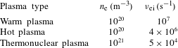
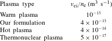
 $n_{\text{e}}\sim 10^{19}~\text{ m}^{-3}$, and contrast typical parameters of our fully ionized gas with those of warm, hot and thermonuclear plasmas.
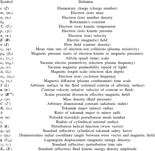
In appendix C, we generalize Alfvén’s theorem on the assumption that the electric field which moves with the fluid does not vanish, but is proportional to the time rate of change of the current density. For a sufficiently low electron number density which varies slowly in time and weakly in space, we find that the frozen-in condition holds true for an effective magnetic field which depends on a finite electron skin depth. In appendix D, we provide a list of definitions for the symbols used throughout the text.
In § 2, we introduce our basic equations. For an ideal (inviscid and perfectly conducting), magnetized plasma, they express mass, momentum and energy conservation. The electric field which moves with the fluid is assumed to be proportional to the time rate of change of the current density. Then, we perform a linear analysis of a static, and time independent equilibrium to derive a general dispersion relation. By considering an axisymmetric equilibrium in a cylindrical tokamak, we realize that its safety factor (and magnetic, rational surfaces) must be defined in terms of the frozen-in, effective magnetic field. Hence, we perform a (divergenceless) helical perturbation on the axisymmetric equilibrium to derive the dispersion relation in the cylindrical tokamak limit.
In § 3, we apply our analytical formulation, derived in the preceding section, to the peaked model which assumes a logarithmic derivative profile for the poloidal component of the equilibrium magnetic field. On the assumption of a parabolic profile for the equilibrium fluid pressure, we succeed in calculating the toroidal component of the equilibrium magnetic field from the equilibrium condition. Thus, we compute the effective fields and safety factor, and identify the rational surfaces. In this formulation, defining the safety factor in terms of the effective field yields a shift in the magnetic surfaces. Finally, we analyse the equilibrium stability from the viewpoint of the system energy. The fluid kinetic energy density amplitude is expressed in terms of a Lagrangian displacement which requires that the perturbation time rate depends on the space coordinates. We find that the instability peak may be three times as high as that predicted on neglect of a finite electron mass. We also find that inertial effects may increase the radius of the stable cylindrical column by two orders of magnitude.
In the concluding section, we summarize this work. We remark that Suydam’s criterion, the stability condition for a helical perturbation mode that is localized arbitrarily close to a cylindrical rational surface, should be examined in the framework of our theory. Drift waves are characterized by frequencies which fall short of that of the ion cyclotron motion,  $\unicode[STIX]{x1D714}_{\text{ci}}$. Those waves are closely related to turbulence in fusion plasmas, and friction of zonal flows. Our analytical formulation predicts that the collision time rate of electrons with ions,
 $\unicode[STIX]{x1D708}_{\text{ei}}$, also falls short of the ion cyclotron frequency,
 $\unicode[STIX]{x1D708}_{\text{ei}}\ll \unicode[STIX]{x1D714}_{\text{ci}}$. However, such an observation does not suffice to characterize the occurrence of drift waves in the framework of our model. There are collisional drift waves with
 $\unicode[STIX]{x1D708}_{\text{ei}}\sim \unicode[STIX]{x1D714}_{\text{ci}}$, which still characterize turbulence at the edge of tokamak devices. Hence, to allow drift waves to be described by our analytical formulation, we prove that it characterizes low frequency, and low wavenumber systems. Therefore, we remark that the framework of our theory may contribute to clarify the interplay of drift waves, turbulence and zonal flows.
2 Analytical formulation
2.1 Basic equations
Consider a fluid, flowing with no source of mass. Thus, the explicit rate of change with time of its mass density,  $\unicode[STIX]{x1D70C}$, shall balance the divergence of the mass current density,
 $\unicode[STIX]{x1D70C}\boldsymbol{v}$,
 $$\begin{eqnarray}\frac{\unicode[STIX]{x2202}\unicode[STIX]{x1D70C}}{\unicode[STIX]{x2202}t}=-\unicode[STIX]{x1D735}\boldsymbol{\cdot }(\unicode[STIX]{x1D70C}\boldsymbol{v}),\end{eqnarray}$$
where  $\boldsymbol{v}$ is the flow field.
If, in addition, that (inviscid) fluid is a magnetized plasma, then the total rate of change with time of the flow field is governed by Euler’s equation,
 $$\begin{eqnarray}\frac{\unicode[STIX]{x2202}\boldsymbol{v}}{\unicode[STIX]{x2202}t}+(\boldsymbol{v}\boldsymbol{\cdot }\unicode[STIX]{x1D735})\boldsymbol{v}=-\frac{1}{\unicode[STIX]{x1D70C}}\unicode[STIX]{x1D735}p+\frac{1}{\unicode[STIX]{x1D70C}}\boldsymbol{J}\times \boldsymbol{B},\end{eqnarray}$$
where  $p$ denotes the fluid pressure. The electric current density,
 $\boldsymbol{J}$, and magnetic field,
 $\boldsymbol{B}$, are related via Ampère’s law,
 $$\begin{eqnarray}\boldsymbol{J}=\frac{1}{\unicode[STIX]{x1D707}_{0}}\unicode[STIX]{x1D735}\times \boldsymbol{B},\end{eqnarray}$$
where  $\unicode[STIX]{x1D707}_{0}$ designates the vacuum magnetic permeability. Substituting (2.3) in (2.2), we obtain
 $$\begin{eqnarray}\frac{\unicode[STIX]{x2202}\boldsymbol{v}}{\unicode[STIX]{x2202}t}+(\boldsymbol{v}\boldsymbol{\cdot }\unicode[STIX]{x1D735})\boldsymbol{v}=-\frac{1}{\unicode[STIX]{x1D70C}}\unicode[STIX]{x1D735}p+\frac{1}{\unicode[STIX]{x1D707}_{0}\unicode[STIX]{x1D70C}}(\unicode[STIX]{x1D735}\times \boldsymbol{B})\times \boldsymbol{B}.\end{eqnarray}$$
Now, assume an adiabatic equation of state,  $p=C\unicode[STIX]{x1D70C}^{\unicode[STIX]{x1D6E4}}$, where
 $C$ stands for a (with appropriate dimension) constant and
 $\unicode[STIX]{x1D6E4}$, for the ratio of specific heats at constant pressure to volume. Hence, mass conservation, equation (2.1), implies
 $$\begin{eqnarray}\frac{\unicode[STIX]{x2202}p}{\unicode[STIX]{x2202}t}+\unicode[STIX]{x1D735}\boldsymbol{\cdot }(p\boldsymbol{v})=-(\unicode[STIX]{x1D6E4}-1)p\unicode[STIX]{x1D735}\boldsymbol{\cdot }\boldsymbol{v}.\end{eqnarray}$$
But, since the fluid is a magnetized plasma, energy conservation requires that the right-hand side of (2.5) also contemplates the source of power density that is responsible to move the electric charges in the medium. Therefore, we correct (2.5) to
 $$\begin{eqnarray}\frac{\unicode[STIX]{x2202}p}{\unicode[STIX]{x2202}t}+\unicode[STIX]{x1D735}\boldsymbol{\cdot }(p\boldsymbol{v})=-(\unicode[STIX]{x1D6E4}-1)[p\unicode[STIX]{x1D735}\boldsymbol{\cdot }\boldsymbol{v}-(\boldsymbol{E}+\boldsymbol{v}\times \boldsymbol{B})\boldsymbol{\cdot }\boldsymbol{J}].\end{eqnarray}$$
If the plasma resistivity,  $\unicode[STIX]{x1D702}$, is finite, then, according to Ohm’s law, the electric field which moves with the fluid,
 $\boldsymbol{E}+\boldsymbol{v}\times \boldsymbol{B}=\unicode[STIX]{x1D702}\boldsymbol{J}$. That leads to the occurrence of the term
 $\unicode[STIX]{x1D702}J^{2}$ on the right-hand side of (2.6), thereby describing the Joule effect. On neglect of any finite resistivity, still there remains a mechanical power density, due to the divergence of the flow field. However, in this work, we consider another possibility for Ohm’s law. As shown in appendix A, for a sufficiently low plasma density, the electric field which moves with the fluid may be given by
 $$\begin{eqnarray}\boldsymbol{E}+\boldsymbol{v}\times \boldsymbol{B}=\unicode[STIX]{x1D707}_{0}\unicode[STIX]{x1D6FF}_{\text{e}}^{2}\frac{\unicode[STIX]{x2202}\boldsymbol{J}}{\unicode[STIX]{x2202}t},\end{eqnarray}$$
where  $\unicode[STIX]{x1D6FF}_{\text{e}}$ denotes the electron skin depth. Substituting (2.7) in (2.6), we obtain
 $$\begin{eqnarray}\frac{\unicode[STIX]{x2202}p}{\unicode[STIX]{x2202}t}+\boldsymbol{v}\boldsymbol{\cdot }\unicode[STIX]{x1D735}p=-\unicode[STIX]{x1D6E4}p\unicode[STIX]{x1D735}\boldsymbol{\cdot }\boldsymbol{v}+\frac{(\unicode[STIX]{x1D6E4}-1)\unicode[STIX]{x1D6FF}_{\text{e}}^{2}}{\unicode[STIX]{x1D707}_{0}}\left(\unicode[STIX]{x1D735}\times \frac{\unicode[STIX]{x2202}\boldsymbol{B}}{\unicode[STIX]{x2202}t}\right)\boldsymbol{\cdot }(\unicode[STIX]{x1D735}\times \boldsymbol{B}),\end{eqnarray}$$
where use has been made again of Ampère’s law, equation (2.3).
Finally, the explicit rate of change with time of the magnetic field is governed by Faraday’s law,
 $$\begin{eqnarray}\frac{\unicode[STIX]{x2202}\boldsymbol{B}}{\unicode[STIX]{x2202}t}=-\unicode[STIX]{x1D735}\times \boldsymbol{E}.\end{eqnarray}$$
Substituting (2.3) and (2.7) in (2.9), we obtain
 $$\begin{eqnarray}\frac{\unicode[STIX]{x2202}\boldsymbol{B}}{\unicode[STIX]{x2202}t}=\unicode[STIX]{x1D735}\times (\boldsymbol{v}\times \boldsymbol{B})-\unicode[STIX]{x1D6FF}_{\text{e}}^{2}\unicode[STIX]{x1D735}\times \left(\unicode[STIX]{x1D735}\times \frac{\unicode[STIX]{x2202}\boldsymbol{B}}{\unicode[STIX]{x2202}t}\right).\end{eqnarray}$$
Equations (2.1), (2.4), (2.8) and (2.10) are the basic equations of this work.
2.2 Linear analysis of static, time independent equilibrium
Regard the fluid to be in a static,  $\boldsymbol{v}_{0}=0$, time independent,
 $\unicode[STIX]{x2202}/\unicode[STIX]{x2202}t\mid _{0}=0$, state of equilibrium, where the subscript ‘0’ stands for ‘equilibrium’. Thus, equations (2.1), (2.8) and (2.10), all become automatically satisfied, and (2.4) implies the condition
 $$\begin{eqnarray}\unicode[STIX]{x1D735}p_{0}=\frac{1}{\unicode[STIX]{x1D707}_{0}}(\unicode[STIX]{x1D735}\times \boldsymbol{B}_{0})\times \boldsymbol{B}_{0}\end{eqnarray}$$
must hold true. About the state of equilibrium of the fluid, described by (2.11), we consider a ‘small’ time perturbation of any equilibrium field,  $f_{0}$ say, namely
 $$\begin{eqnarray}f(t)=f_{0}+f_{1}\exp (\unicode[STIX]{x1D6FE}t),\end{eqnarray}$$
where  $f_{1}$ denotes a (uniquely space dependent) perturbation field, and
 $\unicode[STIX]{x1D6FE}$ designates a time rate. The perturbation is small in the sense that the amplitude of any perturbation field is assumed to be much smaller than that of its corresponding equilibrium field,
 $|f_{1}|\ll |f_{0}|$. But this means that we may substitute (2.12) in (2.1), (2.4), (2.8) and (2.10), and, subsequently, by neglecting terms of
 $O(f_{1}^{2})$, obtain the linear equations
 $$\begin{eqnarray}\left.\begin{array}{@{}c@{}}\unicode[STIX]{x1D6FE}\unicode[STIX]{x1D70C}_{1}+\boldsymbol{v}_{1}\boldsymbol{\cdot }\unicode[STIX]{x1D735}\unicode[STIX]{x1D70C}_{0}=-\unicode[STIX]{x1D70C}_{0}\unicode[STIX]{x1D735}\boldsymbol{\cdot }\boldsymbol{v}_{1},\\ \unicode[STIX]{x1D70C}_{0}\unicode[STIX]{x1D6FE}\boldsymbol{v}_{1}=-\unicode[STIX]{x1D735}p_{1}+{\displaystyle \frac{1}{\unicode[STIX]{x1D707}_{0}}}(\unicode[STIX]{x1D735}\times \boldsymbol{B}_{0})\times \boldsymbol{B}_{1}+{\displaystyle \frac{1}{\unicode[STIX]{x1D707}_{0}}}(\unicode[STIX]{x1D735}\times \boldsymbol{B}_{1})\times \boldsymbol{B}_{0},\\ \unicode[STIX]{x1D6FE}p_{1}+\boldsymbol{v}_{1}\boldsymbol{\cdot }\unicode[STIX]{x1D735}p_{0}=-\unicode[STIX]{x1D6E4}p_{0}\unicode[STIX]{x1D735}\boldsymbol{\cdot }\boldsymbol{v}_{1}+{\displaystyle \frac{(\unicode[STIX]{x1D6E4}-1)\unicode[STIX]{x1D6FE}\unicode[STIX]{x1D6FF}_{\text{e}}^{2}}{\unicode[STIX]{x1D707}_{0}}}(\unicode[STIX]{x1D735}\times \boldsymbol{B}_{1})\boldsymbol{\cdot }(\unicode[STIX]{x1D735}\times \boldsymbol{B}_{0}),\\ \unicode[STIX]{x1D6FE}\boldsymbol{B}_{1}=\unicode[STIX]{x1D735}\times (\boldsymbol{v}_{1}\times \boldsymbol{B}_{0})-\unicode[STIX]{x1D6FE}\unicode[STIX]{x1D6FF}_{\text{e}}^{2}\unicode[STIX]{x1D735}\times (\unicode[STIX]{x1D735}\times \boldsymbol{B}_{1}).\end{array}\right\}\end{eqnarray}$$
From (2.13), we see at once that  $\unicode[STIX]{x1D70C}_{1}$ is fully determined by
 $\unicode[STIX]{x1D70C}_{0}$, and
 $\boldsymbol{v}_{1}$, and also that the former quantity decouples from the remaining ones, both equilibrium and perturbation fields. Hence, we do not worry any longer about
 $\unicode[STIX]{x1D70C}_{1}$ in this work. Further,
 $p_{1}$ may be easily eliminated from our analysis by multiplying the second of (2.13) by
 $\unicode[STIX]{x1D6FE}$, taking the gradient of the third of (2.13) and, subsequently, suitably adding the resulting equations, to obtain
 $$\begin{eqnarray}\displaystyle \unicode[STIX]{x1D70C}_{0}\unicode[STIX]{x1D6FE}^{2}\boldsymbol{v}_{1}-\unicode[STIX]{x1D735}(\boldsymbol{v}_{1}\boldsymbol{\cdot }\unicode[STIX]{x1D735}p_{0}) & = & \displaystyle \frac{\unicode[STIX]{x1D6FE}}{\unicode[STIX]{x1D707}_{0}}(\unicode[STIX]{x1D735}\times \boldsymbol{B}_{0})\times \boldsymbol{B}_{1}+\frac{\unicode[STIX]{x1D6FE}}{\unicode[STIX]{x1D707}_{0}}(\unicode[STIX]{x1D735}\times \boldsymbol{B}_{1})\times \boldsymbol{B}_{0}+\unicode[STIX]{x1D6E4}\unicode[STIX]{x1D735}(p_{0}\unicode[STIX]{x1D735}\boldsymbol{\cdot }\boldsymbol{v}_{1})\nonumber\\ \displaystyle & & \displaystyle -\,\frac{(\unicode[STIX]{x1D6E4}-1)\unicode[STIX]{x1D6FE}\unicode[STIX]{x1D6FF}_{\text{e}}^{2}}{\unicode[STIX]{x1D707}_{0}}\unicode[STIX]{x1D735}[(\unicode[STIX]{x1D735}\times \boldsymbol{B}_{1})\boldsymbol{\cdot }(\unicode[STIX]{x1D735}\times \boldsymbol{B}_{0})].\end{eqnarray}$$
Finally, by suitably taking the scalar product of (2.14) with the fourth of (2.13), we obtain the general dispersion relation
 $$\begin{eqnarray}\displaystyle & & \displaystyle \unicode[STIX]{x1D707}_{0}[\unicode[STIX]{x1D70C}_{0}\unicode[STIX]{x1D6FE}^{2}\boldsymbol{v}_{1}-\unicode[STIX]{x1D735}(\boldsymbol{v}_{1}\boldsymbol{\cdot }\unicode[STIX]{x1D735}p_{0})-\unicode[STIX]{x1D6E4}\unicode[STIX]{x1D735}(p_{0}\unicode[STIX]{x1D735}\boldsymbol{\cdot }\boldsymbol{v}_{1})]\boldsymbol{\cdot }[\boldsymbol{B}_{1}+\unicode[STIX]{x1D6FF}_{\text{e}}^{2}\unicode[STIX]{x1D735}\times (\unicode[STIX]{x1D735}\times \boldsymbol{B}_{1})]\nonumber\\ \displaystyle & & \displaystyle \quad =[(\unicode[STIX]{x1D735}\times \boldsymbol{B}_{0})\times \boldsymbol{B}_{1}+(\unicode[STIX]{x1D735}\times \boldsymbol{B}_{1})\times \boldsymbol{B}_{0}]\boldsymbol{\cdot }[\unicode[STIX]{x1D735}\times \left(\boldsymbol{v}_{1}\times \boldsymbol{B}_{0}\right)]\nonumber\\ \displaystyle & & \displaystyle \qquad -\,(\unicode[STIX]{x1D6E4}-1)\unicode[STIX]{x1D6FF}_{\text{e}}^{2}\{\unicode[STIX]{x1D735}[(\unicode[STIX]{x1D735}\times \boldsymbol{B}_{1})\boldsymbol{\cdot }(\unicode[STIX]{x1D735}\times \boldsymbol{B}_{0})]\}\boldsymbol{\cdot }[\unicode[STIX]{x1D735}\times (\boldsymbol{v}_{1}\times \boldsymbol{B}_{0})].\end{eqnarray}$$
2.3 Axisymmetric equilibrium in a cylindrical tokamak
In this work, we are interested in developing a linear stability analysis for a static, time independent state of equilibrium for a plasma with a sufficiently low density which, for a reason that soon will be clear, varies slowly in time and weakly in space. As an appropriate framework, we consider a large aspect-ratio, one-genus torus topology, one that, sometimes, is referred to as a ‘cylindrical tokamak’. The aspect ratio,  $A$, of a one-genus torus is defined as the ratio of its toroidal, (major)
 $R_{0}$, to poloidal, (minor)
 $r_{0}$, radii, (Wesson Reference Wesson2004; White Reference White2014)
 $$\begin{eqnarray}A\equiv \frac{R_{0}}{r_{0}}.\end{eqnarray}$$
This means that a large aspect-ratio, one-genus torus is one whose radii shall satisfy the condition  $R_{0}\gg r_{0}$, or, equivalently,
 $A\gg 1$. In such a limit, the one-genus toroidal topology may be (locally) approximated by the geometry of a cylinder, hence the above mentioned term cylindrical tokamak. We adopt cylindrical coordinates,
 $(r,\unicode[STIX]{x1D703},z)$, in such a way that the radial coordinate,
 $0\leqslant r\leqslant r_{0}$, denotes the radius of the poloidal (circular) cross-section, the azimuthal coordinate,
 $0\leqslant \unicode[STIX]{x1D703}\leqslant 2\unicode[STIX]{x03C0}$, describes the poloidal angle and the axial coordinate,
 $0\leqslant z\leqslant 2\unicode[STIX]{x03C0}R_{0}$, designates the arc length along the toroidal axis.
Given the above considerations, regard our plasma, with its slowly and weakly varying low density, in a cylindrical tokamak. Assume that it is in a static, time independent state of equilibrium and the equilibrium fields are axisymmetric with respect to the cylindrical axis. In other words, suppose that the equilibrium fields depend uniquely on the radial coordinate,  $f_{0}=f_{0}(r)$. As a result, equation (2.11) implies
 $p_{0}=p_{0}(r)$ and
 $\boldsymbol{B}_{0}(r,\unicode[STIX]{x1D703})=\hat{\unicode[STIX]{x1D703}}B_{\unicode[STIX]{x1D703}}(r)+\hat{z}B_{z}(r)$. However, as shown in appendix C, for a plasma with a sufficiently low density, which varies slowly in time and weakly in space, we may define an ‘effective’ magnetic field,
 $$\begin{eqnarray}\boldsymbol{B}^{\text{eff}}\equiv \boldsymbol{B}-\unicode[STIX]{x1D6FF}_{\text{e}}^{2}\unicode[STIX]{x1D6FB}^{2}\boldsymbol{B},\end{eqnarray}$$
effective in the sense that it satisfies a generalized Alfvén’s theorem,
 $$\begin{eqnarray}\frac{\text{d}}{\text{d}t}\int _{S}\boldsymbol{B}^{\text{eff}}\boldsymbol{\cdot }\text{d}\boldsymbol{S}=0,\end{eqnarray}$$
where  $S$ is a surface, whose contour moves with the fluid. Thus, in view of the axisymmetry hypothesis, it follows from (2.17) that the equilibrium effective magnetic field may be read as
 $\boldsymbol{B}_{0}^{\text{eff}}(r,\unicode[STIX]{x1D703})=\hat{\unicode[STIX]{x1D703}}B_{\unicode[STIX]{x1D703}}^{\text{eff}}(r)+\hat{z}B_{z}^{\text{eff}}(r)$, whose azimuthal,
 $B_{\unicode[STIX]{x1D703}}^{\text{eff}}$, and axial,
 $B_{z}^{\text{eff}}$, components are given by
 $$\begin{eqnarray}B_{\unicode[STIX]{x1D703}}^{\text{eff}}=B_{\unicode[STIX]{x1D703}}-\unicode[STIX]{x1D6FF}_{\text{e}}^{2}\frac{\text{d}}{\text{d}r}\left[\frac{1}{r}\frac{\text{d}}{\text{d}r}(rB_{\unicode[STIX]{x1D703}})\right],\quad B_{z}^{\text{eff}}=B_{z}-\unicode[STIX]{x1D6FF}_{\text{e}}^{2}\frac{1}{r}\frac{\text{d}}{\text{d}r}\left[r\frac{\text{d}}{\text{d}r}(B_{z})\right].\end{eqnarray}$$
It should be noticed that the absence of any finite radial component for the equilibrium effective magnetic field implies its lines of force are twisted, winding curves, lying on nested, coaxial cylindrical surfaces, the so-called magnetic surfaces.
The reason why we make a point of considering a slowly and weakly varying low density is that the so-called safety factor,  $q$, of a cylindrical tokamak may be appropriately redefined with basis on the equilibrium effective magnetic field, (see again Wesson (Reference Wesson2004), and White (Reference White2014))
 $$\begin{eqnarray}q(r)\equiv \frac{rB_{z}^{\text{eff}}(r)}{R_{0}B_{\unicode[STIX]{x1D703}}^{\text{eff}}(r)}.\end{eqnarray}$$
The safety factor of a cylindrical tokamak quantifies the number  $n$ of turns of the axial component,
 $B_{z}^{\text{eff}}$, around the toroidal direction, per unit length (divided by
 $2\unicode[STIX]{x03C0}R_{0}$), during
 $m$ rotations of the azimuthal component,
 $B_{\unicode[STIX]{x1D703}}^{\text{eff}}$, about the poloidal direction, per unit length (divided by
 $2\unicode[STIX]{x03C0}r$). This means that the lines of force of the equilibrium effective magnetic field superpose on the cylindrical magnetic surfaces whose radii,
 $r_{\text{s}}$ say, satisfy the condition
 $$\begin{eqnarray}\frac{n}{R_{0}}B_{z}^{\text{eff}}(r_{\text{s}})=\frac{m}{r_{\text{s}}}B_{\unicode[STIX]{x1D703}}^{\text{eff}}(r_{\text{s}}).\end{eqnarray}$$
Comparison of (2.20) and (2.21) immediately shows that
 $$\begin{eqnarray}q(r_{\text{s}})=\frac{r_{\text{s}}B_{z}^{\text{eff}}(r_{\text{s}})}{R_{0}B_{\unicode[STIX]{x1D703}}^{\text{eff}}(r_{\text{s}})}=\frac{m}{n},\end{eqnarray}$$
which defines the so-called rational surfaces.
2.4 Helical perturbation on axisymmetric equilibrium
According to (2.18), the magnetic flux due to the effective field, through any surface whose contour moves with the fluid, remains frozen within the plasma. This means that any finite flow would follow the bending of the lines of force of the equilibrium field on the magnetic surfaces. Such a remark is our motivation to restrict ourselves to the consideration of the most simple perturbation, namely that corresponding to radial (normal to the cylindrical surfaces) stretchings of the lines of force. Thus, in this work, we regard the strictly radial helical perturbation
 $$\begin{eqnarray}\boldsymbol{f}_{1}(r,\unicode[STIX]{x1D703},z)=\hat{r}f_{1}(r)\exp [\imath h(\unicode[STIX]{x1D703},z)],\end{eqnarray}$$
where the function  $h(\unicode[STIX]{x1D703},z)$ is defined as
 $$\begin{eqnarray}h(\unicode[STIX]{x1D703},z)=m\unicode[STIX]{x1D703}-n\frac{z}{R_{0}}.\end{eqnarray}$$
It should be noticed that, by introducing the vector
 $$\begin{eqnarray}\boldsymbol{k}(r,\unicode[STIX]{x1D703})\equiv \unicode[STIX]{x1D735}h(\unicode[STIX]{x1D703},z)=\hat{\unicode[STIX]{x1D703}}\frac{m}{r}-\hat{z}\frac{n}{R_{0}},\end{eqnarray}$$
one may easily check that
 $$\begin{eqnarray}\unicode[STIX]{x1D735}\boldsymbol{\cdot }\boldsymbol{k}(r,\unicode[STIX]{x1D703})=\unicode[STIX]{x1D6FB}^{2}h(\unicode[STIX]{x1D703},z)\equiv 0.\end{eqnarray}$$
In other words,  $h(\unicode[STIX]{x1D703},z)$ is a harmonic function because it satisfies Laplace’s equation.
The vector  $\boldsymbol{k}$, as introduced above, determines the trajectories of maximum stretch of the lines of force on a given cylindrical surface. Hence, no stretch at all of the lines of force shall be observable by following the trajectories determined, for instance, by the vector
 $\hat{r}\times \boldsymbol{k}$, which is perpendicular to
 $\boldsymbol{k}$, but lies on the given cylindrical surface. This means that the cylindrical surface itself may be determined by the double cross-product
 $$\begin{eqnarray}\boldsymbol{B}_{0}^{\text{eff}}\times (\hat{r}\times \boldsymbol{k})=\hat{r}(\boldsymbol{k}\boldsymbol{\cdot }\boldsymbol{B}_{0}^{\text{eff}})-\boldsymbol{k}(\hat{r}\boldsymbol{\cdot }\boldsymbol{B}_{0}^{\text{eff}}).\end{eqnarray}$$
Actually, since  $\hat{r}\bot \boldsymbol{B}_{0}^{\text{eff}}$, equations (2.25) and (2.27) show that the cylindrical surface is fully determined by the scalar product
 $$\begin{eqnarray}(\boldsymbol{k}\boldsymbol{\cdot }\boldsymbol{B}_{0}^{\text{eff}})|_{r}=\frac{m}{r}B_{\unicode[STIX]{x1D703}}^{\text{eff}}(r)-\frac{n}{R_{0}}B_{z}^{\text{eff}}(r),\end{eqnarray}$$
where the subscript ‘ $r$’ emphasizes that the computation is performed at some fixed value of the radial coordinate. Comparison of (2.21) and (2.28) immediately shows that
 $$\begin{eqnarray}(\boldsymbol{k}\boldsymbol{\cdot }\boldsymbol{B}_{0}^{\text{eff}})|_{r_{\text{s}}}=0.\end{eqnarray}$$
Equation (2.29) may be regarded as the condition to be satisfied by a helical perturbation on a given rational surface.
A last, but important, ingredient of our analysis is that, in this work, we just regard divergenceless perturbations,  $\unicode[STIX]{x1D735}\boldsymbol{\cdot }\,\boldsymbol{f}_{1}=0$. Since
 $\boldsymbol{f}_{1}$ only has the radial component, and
 $h$ does not depend on
 $r$, the amplitude
 $f_{1}$ satisfies (see (2.23))
 $$\begin{eqnarray}\frac{\text{d}f_{1}}{\text{d}r}=-\frac{f_{1}}{r}.\end{eqnarray}$$
For the magnetic field,  $\boldsymbol{B}_{1}$, that merely confirms the absence of a magnetic monopole. However, for the flow field,
 $\boldsymbol{v}_{1}$, this means that the perturbation is incompressible. As a result, any release, or dissipation, of power density within the system shall be uniquely attributed to the electric field which moves with the fluid (see (2.6)).
2.5 Dispersion relation in the cylindrical tokamak limit
Given the above considered helical perturbation on axisymmetric equilibrium, and after straightforward algebra, the relevant terms in the general dispersion relation, (2.15), may be expanded in terms of the vector  $\imath \boldsymbol{k}$, and perturbation fields
 $\boldsymbol{v}_{1}$, and
 $\boldsymbol{B}_{1}$,
 $$\begin{eqnarray}\left.\begin{array}{@{}c@{}}\unicode[STIX]{x1D735}(\boldsymbol{v}_{1}\boldsymbol{\cdot }\unicode[STIX]{x1D735}p_{0})=\left(\imath \boldsymbol{k}{\displaystyle \frac{\text{d}p_{0}}{\text{d}r}}\right)v_{1}+\left[r{\displaystyle \frac{\text{d}}{\text{d}r}}\left({\displaystyle \frac{1}{r}}{\displaystyle \frac{\text{d}p_{0}}{\text{d}r}}\right)\right]\boldsymbol{v}_{1},\\ \unicode[STIX]{x1D735}\times (\unicode[STIX]{x1D735}\times \boldsymbol{B}_{1})=\left[2{\displaystyle \frac{\unicode[STIX]{x2202}}{\unicode[STIX]{x2202}r}}(\imath \boldsymbol{k})\right]B_{1}-(\imath \boldsymbol{k})^{2}\boldsymbol{B}_{1},\\ (\unicode[STIX]{x1D735}\times \boldsymbol{B}_{1})\times \boldsymbol{B}_{0}=(\imath \boldsymbol{k}\boldsymbol{\cdot }\boldsymbol{B}_{0})\boldsymbol{B}_{1},\\ \unicode[STIX]{x1D735}\times (\boldsymbol{v}_{1}\times \boldsymbol{B}_{0})=-\left(2{\displaystyle \frac{\unicode[STIX]{x2202}\boldsymbol{B}_{0}}{\unicode[STIX]{x2202}r}}\right)v_{1}+(\imath \boldsymbol{k}\boldsymbol{\cdot }\boldsymbol{B}_{0})\boldsymbol{v}_{1}+(\unicode[STIX]{x1D735}\times \boldsymbol{B}_{0})\times \boldsymbol{v}_{1},\\ \unicode[STIX]{x1D735}[(\unicode[STIX]{x1D735}\times \boldsymbol{B}_{1})\boldsymbol{\cdot }(\unicode[STIX]{x1D735}\times \boldsymbol{B}_{0})]=-\left\{r{\displaystyle \frac{\unicode[STIX]{x2202}}{\unicode[STIX]{x2202}r}}\left[{\displaystyle \frac{1}{r}}\imath \boldsymbol{k}\times (\unicode[STIX]{x1D735}\times \boldsymbol{B}_{0})\right]\right\}B_{1}\\ -\imath \boldsymbol{k}\{[\imath \boldsymbol{k}\times (\unicode[STIX]{x1D735}\times \boldsymbol{B}_{0})]\boldsymbol{\cdot }\boldsymbol{B}_{1}\}.\end{array}\right\}\end{eqnarray}$$
Substituting (2.31) in (2.15), and after explicitly performing the indicated computations, we obtain the dispersion relation in the cylindrical tokamak limit,
 $$\begin{eqnarray}\displaystyle & & \displaystyle \unicode[STIX]{x1D707}_{0}\left\{[1+(\boldsymbol{k}\unicode[STIX]{x1D6FF}_{\text{e}})^{2}]\left[\unicode[STIX]{x1D70C}_{0}\unicode[STIX]{x1D6FE}^{2}-r\frac{\text{d}}{\text{d}r}\left(\frac{1}{r}\frac{\text{d}p_{0}}{\text{d}r}\right)\right]+\frac{\text{d}p_{0}}{\text{d}r}\frac{\unicode[STIX]{x2202}}{\unicode[STIX]{x2202}r}[(\boldsymbol{k}\unicode[STIX]{x1D6FF}_{\text{e}})^{2}]\right\}\nonumber\\ \displaystyle & & \displaystyle \quad =-(\boldsymbol{k}\boldsymbol{\cdot }\boldsymbol{B}_{0})^{2}+(\unicode[STIX]{x1D735}\times \boldsymbol{B}_{0})^{2}+2\hat{r}\boldsymbol{\cdot }\left[(\unicode[STIX]{x1D735}\times \boldsymbol{B}_{0})\times \frac{\unicode[STIX]{x2202}\boldsymbol{B}_{0}}{\unicode[STIX]{x2202}r}\right]\nonumber\\ \displaystyle & & \displaystyle \qquad -\,(\unicode[STIX]{x1D6E4}-1)[(\boldsymbol{k}\unicode[STIX]{x1D6FF}_{\text{e}})\boldsymbol{\cdot }\boldsymbol{B}_{0}]r\frac{\unicode[STIX]{x2202}}{\unicode[STIX]{x2202}r}\left\{\frac{1}{r}\hat{r}\boldsymbol{\cdot }[(\boldsymbol{k}\unicode[STIX]{x1D6FF}_{\text{e}})\times (\unicode[STIX]{x1D735}\times \boldsymbol{B}_{0})]\right\}\nonumber\\ \displaystyle & & \displaystyle \qquad -\,(\unicode[STIX]{x1D6E4}-1)[(\boldsymbol{k}\unicode[STIX]{x1D6FF}_{\text{e}})\times (\unicode[STIX]{x1D735}\times \boldsymbol{B}_{0})]^{2}\nonumber\\ \displaystyle & & \displaystyle \qquad +\,(\unicode[STIX]{x1D6E4}-1)\{2\hat{r}\boldsymbol{\cdot }[(\boldsymbol{k}\unicode[STIX]{x1D6FF}_{\text{e}})\times (\unicode[STIX]{x1D735}\times \boldsymbol{B}_{0})]\}\left[(\boldsymbol{k}\unicode[STIX]{x1D6FF}_{\text{e}})\boldsymbol{\cdot }\frac{\unicode[STIX]{x2202}\boldsymbol{B}_{0}}{\unicode[STIX]{x2202}r}\right].\end{eqnarray}$$
It should be noticed that (2.32) allows for uniquely two possibilities: either  $\unicode[STIX]{x1D6FE}^{2}<0$, that is, the equilibrium is stable, or
 $\unicode[STIX]{x1D6FE}^{2}>0$, that is, the equilibrium is unstable.
3 Peaked model
3.1 Radial profiles of equilibrium fields
Define a dimensionless radial coordinate,
 $$\begin{eqnarray}x\equiv \frac{r}{r_{0}},\end{eqnarray}$$
where  $r_{0}$ is the minor radius of the cylindrical tokamak. Since
 $0\leqslant r\leqslant r_{0}$, we see that
 $0\leqslant x\leqslant 1$.
The  $z$-pinch configuration, a cylindrical plasma column that sustains an axial current density and an azimuthal magnetic field, is frequently mentioned in plasma physics textbooks to illustrate the self-consistency of the current density and fluid pressure in a static, time independent, ideal MHD equilibrium (see, for instance, Nishikawa & Wakatani Reference Nishikawa and Wakatani2000). If the current density is uniform, then condition (2.11) shows that the magnetic field increases linearly with
 $r$ and the fluid pressure decreases quadratically with
 $r$. Although that is not the case for a cylindrical tokamak, valuable information on the equilibrium stability of a fusion plasma may often be obtained by adopting a parabolic pressure profile (Wesson Reference Wesson2004; White Reference White2014). Thus, we put
 $$\begin{eqnarray}\frac{p_{0}(x)}{p_{0}(0)}=1-x^{2},\end{eqnarray}$$
where  $p_{0}(0)$ denotes the equilibrium pressure at the cylindrical axis. Note that
 $p_{0}(1)=0$ at the cylindrical wall.
According to our previously considered equation of state,  $p=C\unicode[STIX]{x1D70C}^{\unicode[STIX]{x1D6E4}}$, with
 $C$ standing for a constant, and
 $\unicode[STIX]{x1D6E4}$, for the adiabatic index, we immediately deduce the profile of the mass density,
 $$\begin{eqnarray}\frac{\unicode[STIX]{x1D70C}_{0}(x)}{\unicode[STIX]{x1D70C}_{0}(0)}=(1-x^{2})^{1/\unicode[STIX]{x1D6E4}},\end{eqnarray}$$
where  $\unicode[STIX]{x1D70C}_{0}(0)$ designates the equilibrium density at the cylindrical axis. Consistently,
 $\unicode[STIX]{x1D70C}_{0}(1)=0$ at the cylindrical wall.
Motivated by an intensively investigated, because analytically tractable, profile for the poloidal component of a magnetic field in a cylindrical tokamak, namely the ‘peaked model’, introduced by Furth, Rutherford & Selberg (Reference Furth, Rutherford and Selberg1973), we put
 $$\begin{eqnarray}\frac{B_{\unicode[STIX]{x1D703}}(x)}{B_{\unicode[STIX]{x1D703}}(1)}=\frac{2x}{1+x^{2}},\end{eqnarray}$$
where  $B_{\unicode[STIX]{x1D703}}(1)$ stands for the azimuthal component of the magnetic field at the cylindrical wall. As expected,
 $B_{\unicode[STIX]{x1D703}}(0)=0$ at the cylindrical axis. It should be mentioned that, in its original formulation, the peaked model regards the radial coordinate to be normalized by the so-called ‘current channel width’, not by the minor radius of the cylindrical tokamak. Here, to simplify the approach, we assume that
 $r_{0}$ quantifies the width of the plasma flow. We also remark that the original peaked model neglects any finite gradient in the equilibrium pressure. The reason why we adopt a finite value for
 $\text{d}p_{0}/\text{d}x$ (see (3.2)) shall be clear at the end of this section, where we proceed to a linear stability analysis from an energy viewpoint.
The amplitude of the total equilibrium magnetic field is given by
 $$\begin{eqnarray}B_{0}(x)=\sqrt{B_{\unicode[STIX]{x1D703}}^{2}(x)+B_{z}^{2}(x)},\end{eqnarray}$$
where  $B_{z}(x)$ denotes the axial component. Thus, we may introduce the dimensionless ratio (see appendix A)
 $$\begin{eqnarray}\unicode[STIX]{x1D6FD}_{0}(x)\equiv \frac{2\unicode[STIX]{x1D707}_{0}p_{0}(x)}{B_{0}^{2}(x)},\end{eqnarray}$$
where  $\unicode[STIX]{x1D707}_{0}$ designates the vacuum magnetic permeability. Finally, the condition for static, time independent equilibrium, equation (2.11), together with the radial profiles (3.2) and (3.4), allow us to find the axial component of the equilibrium magnetic field,
 $$\begin{eqnarray}\frac{B_{z}(x)}{B_{0}(0)}=\sqrt{1+\unicode[STIX]{x1D6FD}_{0}(0)x^{2}-\frac{B_{\unicode[STIX]{x1D703}}^{2}(1)}{B_{0}^{2}(0)}\left(\frac{2x}{1+x^{2}}\right)^{2}(2+x^{2})},\end{eqnarray}$$
where  $\unicode[STIX]{x1D6FD}_{0}(0)$ stands for the value of
 $\unicode[STIX]{x1D6FD}_{0}(x)$ at
 $x=0$, and
 $B_{0}(0)$, for the amplitude of the total magnetic field at the cylindrical axis, which is the same as the axial component because the azimuthal one just vanishes there.
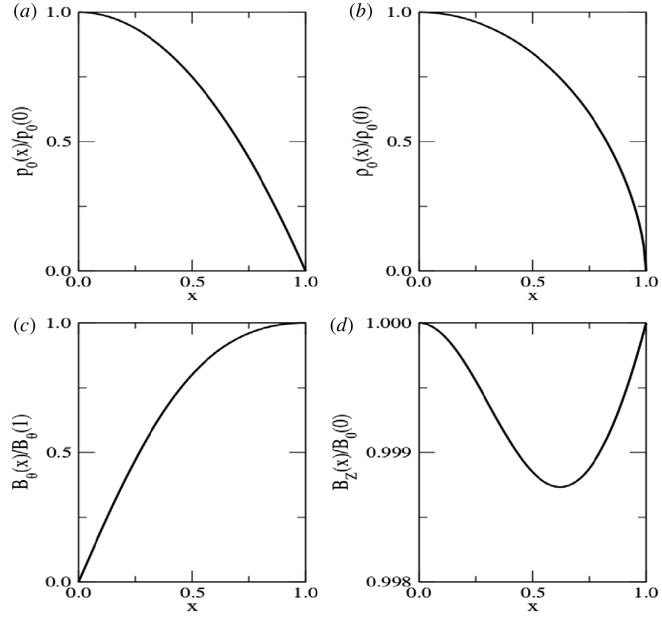
In figure 1, we illustrate the above considered radial profiles of the equilibrium fields.
The radial profiles of the equilibrium fields. (a) The parabolic profile of the fluid pressure, equation (3.2). (b) The profile of the mass density, equation (3.3), for the adiabatic index  $\unicode[STIX]{x1D6E4}=5/3$. (c) The azimuthal component of the magnetic field, equation (3.4). (d) The axial component of the magnetic field, equation (3.7), for
 $\unicode[STIX]{x1D6FD}_{0}(0)=0.01$ (to comply with our assumption that
 $\unicode[STIX]{x1D6FD}_{0}(x)\ll 1$), and
 $B_{\unicode[STIX]{x1D703}}^{2}(1)/B_{0}^{2}(0)=0.01/3$ (as mentioned in the introductory section,
 $B_{\unicode[STIX]{x1D703}}(x)\ll B_{z}(x)$ in a typical tokamak). Note that the relative difference between the maximum (which occurs at both cylindrical axis and wall) and minimum (which occurs at
 $x\sim 0.62$) values of
 $B_{z}(x)$ is of just
 ${\sim}0.12\,\%$.

3.2 Effective fields, safety factor and rational surfaces
We may write the azimuthal, and axial components of the equilibrium effective magnetic field,  $\boldsymbol{B}_{0}^{\text{eff}}$, given by (2.19), with basis on the dimensionless radius,
 $x$, in the form
 $$\begin{eqnarray}\displaystyle \left.\begin{array}{@{}c@{}}{\displaystyle \frac{B_{\unicode[STIX]{x1D703}}^{\text{eff}}(x)}{B_{\unicode[STIX]{x1D703}}(x)}}=1+{\displaystyle \frac{\unicode[STIX]{x1D6FF}_{\text{e}}^{2}}{r_{0}^{2}}}\left[2\left({\displaystyle \frac{2}{1+x^{2}}}\right)^{2}\right],\\ {\displaystyle \frac{B_{z}^{\text{eff}}(x)}{B_{z}(x)}}=1-{\displaystyle \frac{\unicode[STIX]{x1D6FF}_{\text{e}}^{2}}{r_{0}^{2}}}{\displaystyle \frac{B_{0}^{2}(0)}{B_{z}^{2}(x)}}\left[2\unicode[STIX]{x1D6FD}_{0}(0)-{\displaystyle \frac{B_{\unicode[STIX]{x1D703}}^{2}(1)}{B_{0}^{2}(0)}}\left({\displaystyle \frac{2}{1+x^{2}}}\right)^{4}(1-2x^{2})\right]\\ +{\displaystyle \frac{\unicode[STIX]{x1D6FF}_{\text{e}}^{2}}{r_{0}^{2}}}{\displaystyle \frac{B_{0}^{4}(0)}{B_{z}^{4}(x)}}\left[\unicode[STIX]{x1D6FD}_{0}(0)x-{\displaystyle \frac{B_{\unicode[STIX]{x1D703}}^{2}(1)}{B_{0}^{2}(0)}}\left({\displaystyle \frac{2}{1+x^{2}}}\right)^{3}x\right]^{2},\end{array}\right\} & & \displaystyle\end{eqnarray}$$
respectively, where, for simplicity, we have assumed that  $B_{\unicode[STIX]{x1D703}}^{\text{eff}}(x)$, and
 $B_{z}^{\text{eff}}(x)$ are normalized by
 $B_{\unicode[STIX]{x1D703}}(1)$, and
 $B_{0}(0)$, respectively.
Substituting (3.8) in (2.20), we obtain an expression for the safety factor,  $q$, also in terms of
 $x$,
 $$\begin{eqnarray}\frac{q(x)}{q_{0}(x)}=\frac{B_{z}^{\text{eff}}(x)/B_{z}(x)}{B_{\unicode[STIX]{x1D703}}^{\text{eff}}(x)/B_{\unicode[STIX]{x1D703}}(x)},\end{eqnarray}$$
where we have introduced the limit of  $q$ for a vanishingly small electron skin depth,
 $$\begin{eqnarray}q_{0}(x)\equiv \lim _{\unicode[STIX]{x1D6FF}_{\text{e}}\rightarrow 0}q(x)=\frac{xB_{z}(x)}{AB_{\unicode[STIX]{x1D703}}(x)},\end{eqnarray}$$
with  $A$ denoting the aspect ratio of the cylindrical tokamak, defined by (2.16).
Introducing the projections  $(B_{0}\cos \unicode[STIX]{x1D719}_{0})^{\text{eff}}$, and
 $(B_{0}\cos \unicode[STIX]{x1D719}_{0})$ of the effective, and standard, respectively, equilibrium magnetic fields, on the direction of the vector
 $\boldsymbol{k}$ defined by (2.25), one may easily check that (2.28) implies
 $$\begin{eqnarray}\frac{(B_{0}\cos \unicode[STIX]{x1D719}_{0})^{\text{eff}}}{(B_{0}\cos \unicode[STIX]{x1D719}_{0})}=\frac{B_{\unicode[STIX]{x1D703}}^{\text{eff}}(x)/B_{\unicode[STIX]{x1D703}}(x)}{1-q_{0}(x)/(m/n)}+\frac{B_{z}^{\text{eff}}(x)/B_{z}(x)}{1-[q_{0}(x)/(m/n)]^{-1}},\end{eqnarray}$$
where the fraction  $m/n$ determines the rational surfaces (see (2.22)).
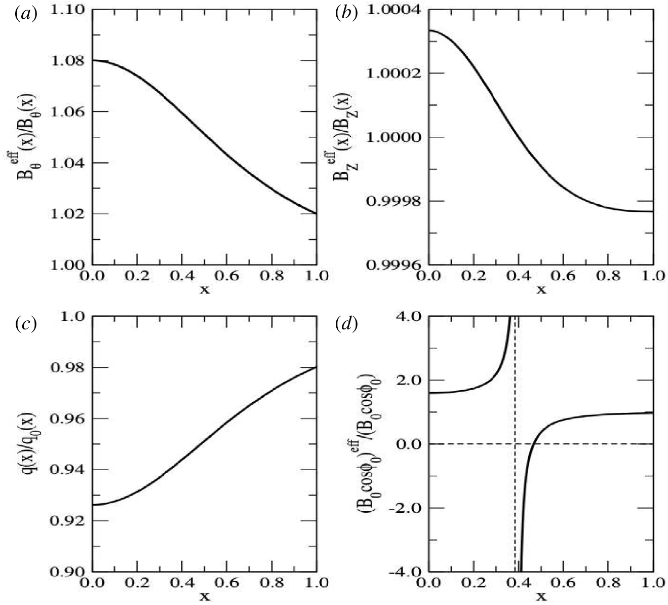
In figure 2, we illustrate the behaviour of the above derived expressions for the effective fields, safety factor and field projections throughout the circular cross-section of the cylindrical tokamak.
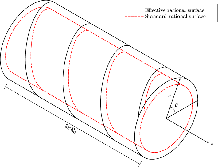
In figure 3, we illustrate the shift of a magnetic surface as a consequence of including a finite electron mass in the peaked model.
Here, we assume that  $\unicode[STIX]{x1D6FF}_{\text{e}}^{2}/r_{0}^{2}=0.01$ (small electron skin depth),
 $A=10$ (large aspect-ratio tokamak) and
 $m/n=1$ (fundamental rational surface). The values of
 $\unicode[STIX]{x1D6FD}_{0}(0)$ and
 $B_{\unicode[STIX]{x1D703}}^{2}(1)/B_{0}^{2}(0)$ are the same as those considered in figure 1. (a) The ratio of effective to standard azimuthal components of the magnetic field, both normalized to
 $B_{\unicode[STIX]{x1D703}}(1)$, the first of (3.8). Finite electron mass effects are larger close to the axis, and smaller close to the wall. The effective is always larger than the standard component. The curve exhibits a saddle point at
 $x\sim 0.39$. (b) The ratio of effective to standard axial components of the magnetic field, both normalized to
 $B_{0}(0)$, the second of (3.8). Finite electron mass effects are larger close to both axis and wall. The effective approaches the standard component at the same saddle point as before,
 $x\sim 0.39$. (c) The ratio of the safety factor to its vanishing electron mass limit, equation (3.9). Finite electron mass effects are larger close to the axis, and smaller close to the wall. The safety factor is always smaller than its vanishing electron mass limit, which means that both effective and standard rational surfaces cannot coalesce into one unique manifold. The curve exhibits a saddle point, again, at
 $x\sim 0.39$. (d) The ratio of projections of effective to standard equilibrium magnetic fields on the direction of the vector
 $\boldsymbol{k}$, equation (3.11). Finite electron mass effects are larger close to the axis, and smaller close to the wall. Close to the axis, the projections are parallel to each other. At
 $x\sim 0.39$, the curve diverges, indicating the occurrence of a standard rational surface. As
 $x$ increases, the projections become antiparallel to each other. At
 $x\sim 0.46$, the curve intercepts the horizontal axis, indicating the occurrence of an effective rational surface. As
 $x$ approaches the wall, the projections become again parallel to each other, and they finally superpose on the wall.

Illustration of the shift of a magnetic surface as a consequence of including a finite electron mass in the peaked model. In accordance with figure 2(d), the internal (external) cylindrical shell represents the standard (effective) rational surface. The helical lines of force for the magnetic fields are sketched on both shells.

3.3 Energy considerations on stability analysis
The fluid kinetic energy density is given by
 $$\begin{eqnarray}K={\textstyle \frac{1}{2}}\unicode[STIX]{x1D70C}v^{2},\end{eqnarray}$$
where  $\unicode[STIX]{x1D70C}$, and
 $\boldsymbol{v}$, are the mass density, and flow field, respectively. Now, if the fluid slightly departs from a state of equilibrium, as indicated by (2.12), then (3.12) implies
 $$\begin{eqnarray}K={\textstyle \frac{1}{2}}(\unicode[STIX]{x1D70C}_{0}+\unicode[STIX]{x1D70C}_{1})(\boldsymbol{v}_{0}+\boldsymbol{v}_{1})^{2},\end{eqnarray}$$
where the subscripts ‘0’, and ‘1’, denote ‘equilibrium’, and ‘perturbation’, respectively. Finally, on the assumption that the fluid was in a static state of equilibrium ( $\boldsymbol{v}_{0}=0$), equation (3.13) reduces to
 $$\begin{eqnarray}K={\textstyle \frac{1}{2}}\unicode[STIX]{x1D70C}_{0}v_{1}^{2},\end{eqnarray}$$
where the third-order perturbation term  $\unicode[STIX]{x1D70C}_{1}v_{1}^{2}$ has been neglected.
The perturbation flow may be expressed in terms of a Lagrangian displacement,  $\unicode[STIX]{x1D743}$ say, by putting (Bennett Reference Bennett2006)
 $$\begin{eqnarray}\boldsymbol{v}_{1}=\frac{\unicode[STIX]{x2202}\unicode[STIX]{x1D743}}{\unicode[STIX]{x2202}t}.\end{eqnarray}$$
In the Lagrangian formulation of continuum mechanics, a change in the configuration of a volume element is described by a displacement field. The displacement field of the volume element consists in two components: a rigid-body displacement and a deformation. A rigid-body displacement is simultaneously composed of a translation and a rotation of the volume element, with no change in its shape nor in its size. A deformation is the result of a change in shape and/or in size of the volume element. The vector field  $\unicode[STIX]{x1D743}$, which joins two vector positions of a given volume element, from the previously undeformed to the presently deformed configurations, is called a Lagrangian displacement. Here, for our purposes, it proves convenient to normalize
 $\unicode[STIX]{x1D743}$ by the minor radius,
 $r_{0}$, of the cylindrical tokamak. Thus, we rewrite (3.15) as
 $$\begin{eqnarray}\boldsymbol{v}_{1}=r_{0}\frac{\unicode[STIX]{x2202}\unicode[STIX]{x1D743}}{\unicode[STIX]{x2202}t},\end{eqnarray}$$
where  $\unicode[STIX]{x1D743}$ denotes, now, a dimensionless vector field.
To comply with our previously assumed time dependence of the perturbation fields, as indicated again by (2.12), we put
 $$\begin{eqnarray}\unicode[STIX]{x1D743}(x,t)=\unicode[STIX]{x1D743}(x)\exp (\unicode[STIX]{x1D6FE}t),\end{eqnarray}$$
where  $x$ is the dimensionless radius, as defined by (3.1). But, at this point, one must be cautious. In the Eulerian formulation, that we used up to this paragraph, the observer is at the origin of a rest frame, and regards the state and flow of a volume element as projections of those element position and velocity, respectively, on its own coordinate system. This means that the observer measures a time rate
 $\unicode[STIX]{x1D6FE}=\text{const}$. On the other hand, in the Lagrangian formulation, that we introduce in this paragraph, the state and flow of a volume element are regarded as the position and velocity, respectively, of the proper observer which moves with the fluid. This means that, now, the observer measures a time rate
 $\unicode[STIX]{x1D6FE}=\unicode[STIX]{x1D6FE}(x)$.
Given the above considerations, we substitute (3.17) in (3.16), and, subsequently, the resulting equation in (3.14), to obtain
 $$\begin{eqnarray}K(x,t)=K(x)\unicode[STIX]{x1D709}^{2}(x,t),\end{eqnarray}$$
where we have identified the kinetic energy density amplitude,
 $$\begin{eqnarray}K(x)={\textstyle \frac{1}{2}}r_{0}^{2}\unicode[STIX]{x1D70C}_{0}(x)\unicode[STIX]{x1D6FE}^{2}(x),\end{eqnarray}$$
as the coefficient of  $K(x,t)$, in the second-order perturbation term
 $\unicode[STIX]{x1D709}^{2}(x,t)$. At the end of the preceding section, we have noticed that our dispersion relation in the cylindrical tokamak limit, equation (2.32), allows for uniquely two possibilities: either
 $\unicode[STIX]{x1D6FE}^{2}<0$, that is, the equilibrium is stable, or
 $\unicode[STIX]{x1D6FE}^{2}>0$, that is, the equilibrium is unstable. Since the constant
 $r_{0}^{2}>0$, and also the function
 $\unicode[STIX]{x1D70C}_{0}(x)>0$ for all
 $x$, that statement may be now rephrased as: ‘for any
 $x$, equation (3.19) allows for uniquely two possibilities: either
 $K(x)<0$, that is, the local equilibrium is stable, or
 $K(x)>0$, that is, the local equilibrium is unstable’. Let us proceed to the computation of
 $K(x)$ in two steps.
First, consider the limit of  $\unicode[STIX]{x1D6FE}$ when
 $\unicode[STIX]{x1D6FF}_{\text{e}}\rightarrow 0$,
 $\unicode[STIX]{x1D6FE}_{0}$ say. In that case, the kinetic energy density amplitude, equation (3.19), approaches
 $$\begin{eqnarray}K_{0}(x)={\textstyle \frac{1}{2}}r_{0}^{2}\unicode[STIX]{x1D70C}_{0}(x)\unicode[STIX]{x1D6FE}_{0}^{2}(x).\end{eqnarray}$$
Thus, by combining (3.20) with the same limit of (2.32), we get
 $$\begin{eqnarray}\displaystyle \frac{K_{0}(x)}{U_{\text{M}}(0)} & = & \displaystyle \frac{B_{\unicode[STIX]{x1D703}}^{2}(1)}{B_{0}^{2}(0)}\left(\frac{2}{1+x^{2}}\right)^{4}x^{2}-\frac{B_{0}^{2}(0)}{B_{z}^{2}(x)}\left[\unicode[STIX]{x1D6FD}_{0}(0)x-\frac{B_{\unicode[STIX]{x1D703}}^{2}(1)}{B_{0}^{2}(0)}\left(\frac{2}{1+x^{2}}\right)^{3}x\right]^{2}\nonumber\\ \displaystyle & & \displaystyle -\,\left[m\frac{B_{\unicode[STIX]{x1D703}}(1)}{B_{0}(0)}\left(\frac{2}{1+x^{2}}\right)-\frac{n}{A}\frac{B_{z}(x)}{B_{0}(0)}\right]^{2}.\end{eqnarray}$$
In (3.21), we have introduced the quantity  $U_{\text{M}}(0)$, the magnetic energy density
 $$\begin{eqnarray}U_{\text{M}}(x)=\frac{B_{0}^{2}(x)}{2\unicode[STIX]{x1D707}_{0}},\end{eqnarray}$$
calculated for the equilibrium magnetic field  $\boldsymbol{B}_{0}(x)$, and, subsequently, evaluated at the cylindrical axis,
 $x=0$. According to (3.2), the unique term, in the limit of (2.32) when
 $\unicode[STIX]{x1D6FF}_{\text{e}}\rightarrow 0$, that depends on
 $p_{0}$, vanishes,
 $$\begin{eqnarray}r\frac{\text{d}}{\text{d}r}\left[\frac{1}{r}\frac{\text{d}p_{0}}{\text{d}r}\right]=\frac{x}{r_{0}}\frac{\text{d}}{\text{d}x}\left[\frac{-2xp_{0}(0)/r_{0}}{x}\right]=0.\end{eqnarray}$$
This explains why it is useless to assume, in the original peaked model, the otherwise useful, in fusion physics, parabolic profile for the equilibrium pressure. That plays no role in the linear stability analysis.
Second, with basis on (2.32) and (3.21), we find the full expression for the kinetic energy density amplitude, equation (3.19), namely
 $$\begin{eqnarray}\displaystyle \frac{K(x)}{U_{\text{M}}(0)} & = & \displaystyle \left[\frac{x^{2}}{\unicode[STIX]{x0394}(x)}\right]\left[\frac{K_{0}(x)}{U_{\text{M}}(0)}\right]-\frac{\unicode[STIX]{x1D6FF}_{\text{e}}^{2}}{r_{0}^{2}}\left[\frac{2}{\unicode[STIX]{x0394}(x)}\right]\left[m^{2}\unicode[STIX]{x1D6FD}_{0}(0)\right]\nonumber\\ \displaystyle & & \displaystyle +\,\frac{\unicode[STIX]{x1D6FF}_{\text{e}}^{2}}{r_{0}^{2}}\left[\frac{(\unicode[STIX]{x1D6E4}-1)}{\unicode[STIX]{x0394}(x)}\right]\left[m^{2}F(x)+\frac{n^{2}}{A^{2}}G(x)-m\frac{n}{A}H(x)\right],\end{eqnarray}$$
where we have introduced the abbreviations
 $$\begin{eqnarray}\left.\begin{array}{@{}rcl@{}}\unicode[STIX]{x0394}(x)\, & =\, & x^{2}+{\displaystyle \frac{\unicode[STIX]{x1D6FF}_{\text{e}}^{2}}{r_{0}^{2}}}\left(m^{2}+{\displaystyle \frac{n^{2}}{A^{2}}}x^{2}\right),\\ F(x)\, & =\, & {\displaystyle \frac{B_{\unicode[STIX]{x1D703}}^{2}(1)}{B_{0}^{2}(0)}}\left({\displaystyle \frac{2}{1+x^{2}}}\right)^{4}(1+2x^{2}),\\ G(x)\, & =\, & 2{\displaystyle \frac{B_{0}^{2}(0)}{B_{z}^{2}(x)}}\left[\unicode[STIX]{x1D6FD}_{0}(0)x^{2}-{\displaystyle \frac{B_{\unicode[STIX]{x1D703}}^{2}(1)}{B_{0}^{2}(0)}}\left({\displaystyle \frac{2}{1+x^{2}}}\right)^{3}x^{2}\right]^{2}-3{\displaystyle \frac{B_{\unicode[STIX]{x1D703}}^{2}(1)}{B_{0}^{2}(0)}}\left({\displaystyle \frac{2x}{1+x^{2}}}\right)^{4},\\ H(x)\, & =\, & {\displaystyle \frac{B_{\unicode[STIX]{x1D703}}(1)}{B_{0}(0)}}\left({\displaystyle \frac{2}{1+x^{2}}}\right)^{3}\left[(1+3x^{2}){\displaystyle \frac{B_{z}(x)}{B_{0}(0)}}-3{\displaystyle \frac{B_{\unicode[STIX]{x1D703}}^{2}(1)}{B_{0}^{2}(0)}}\left({\displaystyle \frac{2x}{1+x^{2}}}\right)^{2}x^{2}{\displaystyle \frac{B_{0}(0)}{B_{z}(x)}}\right]\\ \, & \, & +\,{\displaystyle \frac{B_{\unicode[STIX]{x1D703}}(1)}{B_{0}(0)}}\left({\displaystyle \frac{2}{1+x^{2}}}\right)^{2}(1-x^{2}){\displaystyle \frac{B_{0}(0)}{B_{z}(x)}}\left[\unicode[STIX]{x1D6FD}_{0}(0)x^{2}-{\displaystyle \frac{B_{\unicode[STIX]{x1D703}}^{2}(1)}{B_{0}^{2}(0)}}\left({\displaystyle \frac{2}{1+x^{2}}}\right)^{3}x^{2}\right]\\ \, & \, & +\,{\displaystyle \frac{B_{\unicode[STIX]{x1D703}}(1)}{B_{0}(0)}}\left({\displaystyle \frac{2}{1+x^{2}}}\right){\displaystyle \frac{B_{0}^{3}(0)}{B_{z}^{3}(x)}}\left[\unicode[STIX]{x1D6FD}_{0}(0)x^{2}-{\displaystyle \frac{B_{\unicode[STIX]{x1D703}}^{2}(1)}{B_{0}^{2}(0)}}\left({\displaystyle \frac{2}{1+x^{2}}}\right)^{3}x^{2}\right]^{2}.\end{array}\right\}\end{eqnarray}$$
According to (3.2), the unique term, proportional to  $\unicode[STIX]{x1D6FF}_{\text{e}}$ in (2.32), that depends on
 $p_{0}$, does not vanish,
 $$\begin{eqnarray}\frac{\text{d}p_{0}}{\text{d}r}=-\frac{2xp_{0}(0)}{r_{0}}\neq 0.\end{eqnarray}$$
This explains why we have introduced, in our formulation, the parabolic profile for the equilibrium pressure. This plays a significant role in the linear stability analysis.
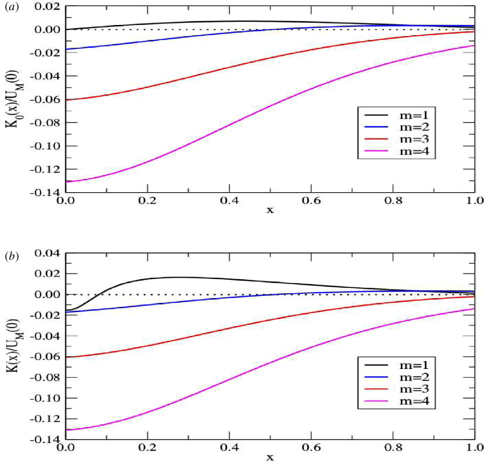
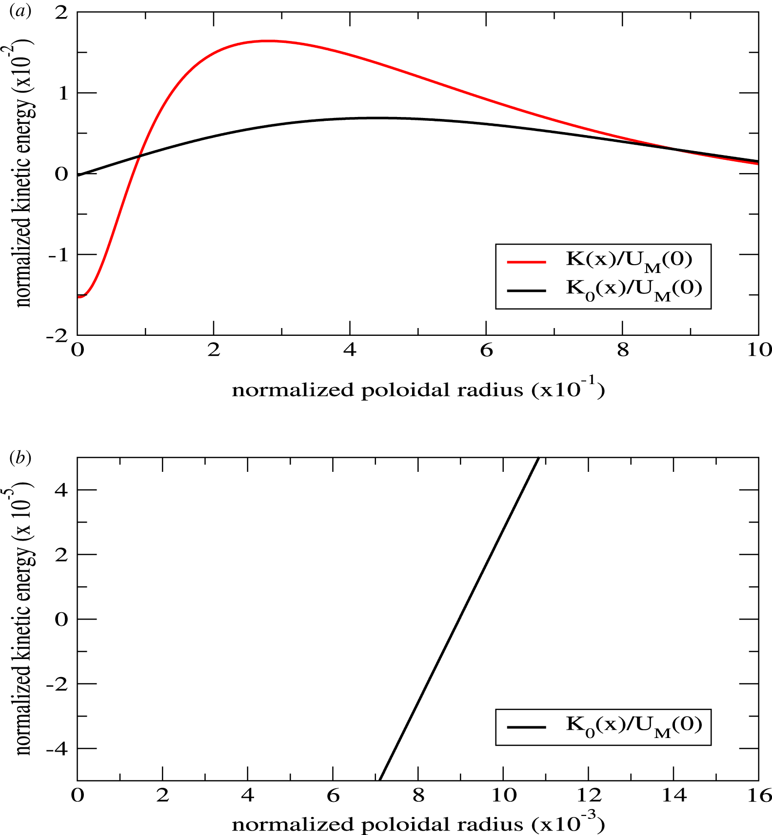
In figure 4, we illustrate the distribution of the kinetic energy density amplitude on the cylindrical surfaces for the first few lowest modes of the helical perturbation. Note that the unique perturbation mode which is effectively affected by the consideration of a finite electron mass is the fundamental one,  $m=n=1$.
In figure 5, we display a close-up view of figure 4 for the fundamental rational surface  $m=n=1$. Note that finite electron mass effects may increase the radius of the stable cylindrical column, as predicted by the peaked model, by two orders of magnitude. Also note that the instability peak may be three times as high as the one predicted by that model on neglect of any finite electron mass.
The distribution of the kinetic energy density amplitude on the cylindrical surfaces for the first few lowest modes of the helical perturbation. The toroidal mode and adiabatic index are fixed to  $n=1$ and
 $\unicode[STIX]{x1D6E4}=5/3$, respectively. The values of
 $\unicode[STIX]{x1D6FD}_{0}(0)$ and
 $B_{\unicode[STIX]{x1D703}}^{2}(1)/B_{0}^{2}(0)$, and, of
 $\unicode[STIX]{x1D6FF}_{\text{e}}^{2}/r_{0}^{2}$ and
 $A$ are the same as those considered in figures 1 and 2, respectively. (a) The limit for a vanishingly small electron skin depth,
 $K_{0}(x)$, equation (3.21). (b) The full expression,
 $K(x)$, equation (3.24).

A close-up view of figure 4 for the fundamental rational surface  $m=n=1$. (a) The instability peak may be three times as high as that predicted on neglect of a finite electron mass. (b) Inertial effects may increase the radius of the stable cylindrical column by two orders of magnitude.

A last note, on the determination of the time rate  $\unicode[STIX]{x1D6FE}$, in the framework of our approach. As one may easily check, in regard to (3.19), the finding of the kinetic energy density amplitude
 $K$, as given by (3.24), does not univocally determine
 $\unicode[STIX]{x1D6FE}$. That is as such because one still needs to accurately provide the equilibrium mass density
 $\unicode[STIX]{x1D70C}_{0}$, for all values of the dimensionless radius
 $x$. However, according to (3.3), in the limit
 $x\rightarrow 1$, the mass density
 $\unicode[STIX]{x1D70C}_{0}\rightarrow 0$, which implies
 $\unicode[STIX]{x1D6FE}^{2}\rightarrow \pm \infty$, for a finite
 $K$. This means that (3.24) is accurate, except close to the cylindrical tokamak wall. In order to correct such a result, one must consider a finite fluid viscosity, which might be important in the limit
 $x\rightarrow 1$, thereby leading to the formation of a viscous boundary layer, close to the tokamak wall. Such a development is postponed to a further communication.
4 Conclusion
We have rescaled the generalized Ohm’s law, and, subsequently, rewritten its coefficients in terms of four independent factors that are given by plasma parameters. Thus, we have considered the approximations on those factors that imply the electric field which moves with the fluid be proportional to the time rate of change of the current density, the constant of proportionality describing inertial effects due to a finite electron mass.
We have shown that the above mentioned approximations are satisfied by a sufficiently low electron number density. We have also shown that the electron–ion collision frequency,  $\unicode[STIX]{x1D708}_{\text{ei}}$, is much smaller than the ion cyclotron frequency,
 $\unicode[STIX]{x1D714}_{\text{ci}}$. Combination of that condition with Lawson criterion for a typical deuterium–tritium fusion in ITER has revealed a lower bound for the geometric mean of the confinement time,
 $\unicode[STIX]{x1D70F}_{\text{C}}$, and collision interval,
 $\sqrt{\unicode[STIX]{x1D70F}_{\text{C}}/\unicode[STIX]{x1D708}_{\text{ei}}}\gg 10^{-5}~\text{s}$. For that reaction, we have estimated that the electron number density
 $n_{\text{e}}\sim 10^{19}~\text{ m}^{-3}$, and contrasted typical parameters of our fully ionized gas with those of warm, hot and thermonuclear plasmas.
We have generalized Alfvén’s theorem on the assumption that the electric field which moves with the fluid does not vanish, but be proportional to the time rate of change of the current density. For a sufficiently low  $n_{\text{e}}$ which varies slowly in time and weakly in space, we have found that the frozen-in condition holds true for an effective magnetic field which depends on a finite electron skin depth.
For an ideal (inviscid and perfectly conducting), magnetized plasma, we have performed a linear analysis of a static, and time independent equilibrium to derive a general dispersion relation. By considering an axisymmetric equilibrium in a cylindrical tokamak, we have realized that its safety factor (and magnetic, rational surfaces) must be defined in terms of the frozen-in, effective magnetic field. Hence, we have performed a (divergenceless) helical perturbation on the axisymmetric equilibrium to derive the dispersion relation in the cylindrical tokamak limit.
We have applied our analytical formulation to the peaked model which assumes a logarithmic derivative profile for the poloidal component of the equilibrium magnetic field. On the assumption of a parabolic profile for the equilibrium fluid pressure, we have succeeded in calculating the toroidal component of the equilibrium magnetic field from the equilibrium condition. Thus, we have computed the effective fields and safety factor, and identified the rational surfaces. In this formulation, defining the safety factor in terms of the effective field yields a shift in the magnetic surfaces.
Finally, we have analysed the equilibrium stability from the viewpoint of the system energy. The fluid kinetic energy density amplitude has been expressed in terms of a Lagrangian displacement which requires that the perturbation time rate depends on the space coordinates. We have found that the instability peak may be three times as high as that predicted on neglect of a finite electron mass. We have also found that inertial effects may increase the radius of the stable cylindrical column by two orders of magnitude.
The linear stability analysis of ideal MHD equilibria is successfully described by the so-called energy principle approach, as originally introduced by Lundquist (Reference Lundquist1952), and, later on, extended by Bernstein et al. (Reference Bernstein, Frieman, Kruskal and Kulsrud1958), to include plasma boundary conditions. According to that principle, the stability of the system is determined by examining the sign of an arbitrary change in the potential energy of the fluid, caused by a small perturbation of the equilibrium fields. The system is stable if that change is not negative for all allowable virtual displacements, satisfying the relevant boundary conditions.
The stability condition for a helical perturbation mode that is localized arbitrarily close to a cylindrical rational surface is commonly referred to as Suydam’s criterion (Suydam Reference Suydam1958), which depends on the safety factor of a cylindrical tokamak. The criterion was extended by Goedbloed (Reference Goedbloed1973), to include a finite pressure gradient which our theory already contemplates. However, Gupta, Callen & Hegna (Reference Gupta, Callen and Hegna2002) claimed that the criterion would not be very restrictive, since perturbation modes could be easily stabilized by finite ion Larmor radius effects.
Given the above considerations, we think that Suydam’s criterion should be examined in the framework of our theory.
Drift waves are characterized by frequencies which fall short of that of the ion cyclotron motion,  $\unicode[STIX]{x1D714}_{\text{ci}}$ (Miyamoto Reference Miyamoto2016). From the 1970s to the 1990s, it was tacitly accepted that low-amplitude drift-wave turbulence could not actually prevent the complacency of the critical Lawson condition for deuterium–tritium ignition,
 $n_{\text{e}}\unicode[STIX]{x1D70F}_{\text{C}}\sim 1.5\times 10^{20}~\text{m}^{-3}~\text{s}$, where
 $n_{\text{e}}$, and
 $\unicode[STIX]{x1D70F}_{\text{C}}$ are the electron number density, and plasma confinement time, respectively (Ongena et al. Reference Ongena, Koch, Wolf and Zohm2016). Today, the plasma community realizes that a mere increase in thermal energy does not suffice to achieve the ignition state, because plasma heating substantially reinforces both the turbulence level and development of coherent structures, thereby gravely degrading the confinement time (Horton et al. Reference Horton, Kim, Asp, Hoang, Watanabe and Sugama2008). Those issues are of great interest to ITER, where collisionless transfer of energy from electrons to ions are expected to be meaningful (see
https://www.iter.org/).
It has been suggested that friction of zonal flows may provide a relevant channel for ion heating because, at steady state, work effected by frictional forces must balance that due to turbulence (Zhao & Diamond Reference Zhao and Diamond2012). Numerical simulations indicate that, in the collisionless approximation, the contribution of zonal flows to the kinetic energy prevails over that of turbulence, which may evolve towards highly anisotropic configurations (Pushkarev, Bos & Nazarenko Reference Pushkarev, Bos and Nazarenko2013). Our analytical formulation predicts that the collision time rate of electrons with ions,  $\unicode[STIX]{x1D708}_{\text{ei}}$, also falls short of the ion cyclotron frequency,
 $\unicode[STIX]{x1D708}_{\text{ei}}\ll \unicode[STIX]{x1D714}_{\text{ci}}$ (see condition (B 12) in appendix B). However, such an observation does not suffice to characterize the occurrence of drift waves in the framework of our model.
There are collisional drift waves with  $\unicode[STIX]{x1D708}_{\text{ei}}\sim \unicode[STIX]{x1D714}_{\text{ci}}$, which still characterize turbulence at the edge of tokamak devices (Jorge, Ricci & Loureiro Reference Jorge, Ricci and Loureiro2018). Therefore, in order to allow drift waves and their derivatives, such as the electron temperature gradient, the ion temperature gradient and the universal instability, to be described by our analytical formulation, we must prove that it characterizes low frequency, and low wavenumber systems (Jorge et al. Reference Jorge, Ricci, Brunner, Gamba, Konovets, Loureiro, Perrone and Teixeira2019). In other words, we might show that the time rate
 $\unicode[STIX]{x1D6FE}$, and wavenumber
 $k$ satisfy the conditions
 $\unicode[STIX]{x1D6FE}^{2}\ll \unicode[STIX]{x1D714}_{\text{ci}}^{2}$, and
 $k^{2}\unicode[STIX]{x1D6FF}_{\text{e}}^{2}\ll 1$ (where
 $\unicode[STIX]{x1D6FF}_{\text{e}}$ denotes the electron skin depth), respectively, at the plasma boundary.
According to (B 11) in appendix B, we may write
 $$\begin{eqnarray}\frac{\unicode[STIX]{x1D6FE}^{2}}{\unicode[STIX]{x1D714}_{\text{ci}}^{2}}=\frac{m_{\text{i}}^{2}\unicode[STIX]{x1D6FE}^{2}}{e^{2}B_{0}^{2}}.\end{eqnarray}$$
Thus, with basis on (3.19) and (3.22) in § 3, and (B 6) in appendix B, equation (4.1) may be read as
 $$\begin{eqnarray}\frac{\unicode[STIX]{x1D6FE}^{2}}{\unicode[STIX]{x1D714}_{\text{ci}}^{2}}=\frac{m_{\text{i}}}{m_{\text{e}}}\frac{K(x)}{U_{\text{M}}(0)}\frac{\unicode[STIX]{x1D6FF}_{\text{e}}^{2}}{r_{0}^{2}},\end{eqnarray}$$
where we have considered  $B_{0}=B_{0}(0)$. First, we note that
 $m_{\text{i}}/m_{\text{e}}\sim 10^{3}$. Next, we observe that figures 4 and 5 show that
 $K(x)/U_{\text{M}}(0)\sim 10^{-3}$ in the limit
 $x\rightarrow 1$. Finally, we remark that our numerical treatment assumes that
 $\unicode[STIX]{x1D6FF}_{\text{e}}^{2}/r_{0}^{2}\sim 10^{-2}$. Therefore, equation (4.2) implies
 $\unicode[STIX]{x1D6FE}^{2}\ll \unicode[STIX]{x1D714}_{\text{ci}}^{2}$ at the plasma boundary.
According to (2.25), we may write
 $$\begin{eqnarray}k^{2}\unicode[STIX]{x1D6FF}_{\text{e}}^{2}=\left(\frac{m^{2}}{r^{2}}+\frac{n^{2}}{R_{0}^{2}}\right)\unicode[STIX]{x1D6FF}_{\text{e}}^{2}.\end{eqnarray}$$
Thus, with basis on definitions (2.16) and (3.1), equation (4.3) may be read as
 $$\begin{eqnarray}k^{2}\unicode[STIX]{x1D6FF}_{\text{e}}^{2}=\left(\frac{m^{2}}{x^{2}}+\frac{n^{2}}{A^{2}}\right)\frac{\unicode[STIX]{x1D6FF}_{\text{e}}^{2}}{r_{0}^{2}}.\end{eqnarray}$$
For the fundamental rational surface,  $m=n=1$, on the cylindrical tokamak approximation,
 $A\gg 1$, equation (4.4) implies
 $k^{2}\unicode[STIX]{x1D6FF}_{\text{e}}^{2}\ll 1$ at the plasma boundary,
 $x\rightarrow 1$, provided that
 $\unicode[STIX]{x1D6FF}_{\text{e}}^{2}\ll r_{0}^{2}$.
Given the above considerations, we think that the framework of our theory may contribute to clarify the interplay of drift waves, turbulence and zonal flows.
Acknowledgements
F.E.M.S. acknowledges partial support by FAPESP, Foundation for Support to Research of the State of São Paulo, under grant no. 17/20192-2. B.P.S. acknowledges support by CAPES, Coordination for Improvement of Higher Education Personnel, under a PhD scholarship. The authors are grateful to M. Assunção and R. S. Camargo for the help with the figures.
Appendix A. Generalized Ohm’s law
A.1 Full expression
Consider a fully ionized, isotropic gas composed of electrons (charge  $-e$, mass
 $m_{\text{e}}$, number density
 $n_{\text{e}}$, kinetic temperature
 $T_{\text{e}}$ and velocity
 $\boldsymbol{v}_{\text{e}}$), and one unique ion species (charge
 $Ze$, mass
 $m_{\text{i}}$, number density
 $n_{\text{i}}$, kinetic temperature
 $T_{\text{i}}$ and velocity
 $\boldsymbol{v}_{\text{i}}$). The ionized gas is subjected to electric
 $\boldsymbol{E}$, and magnetic
 $\boldsymbol{B}$ fields. Thus, the time rate of momentum transfer per unit volume to electrons, and ions may be written as (Spitzer Reference Spitzer2006; Somov Reference Somov2013)
 $$\begin{eqnarray}\left.\begin{array}{@{}c@{}}{\displaystyle \frac{\unicode[STIX]{x2202}}{\unicode[STIX]{x2202}t}}(n_{\text{e}}m_{\text{e}}\boldsymbol{v}_{\text{e}})=-\unicode[STIX]{x1D735}p_{\text{e}}-n_{\text{e}}e(\boldsymbol{E}+\boldsymbol{v}_{\text{e}}\times \boldsymbol{B})-n_{\text{e}}m_{\text{e}}\unicode[STIX]{x1D708}_{\text{ei}}(\boldsymbol{v}_{\text{e}}-\boldsymbol{v}_{\text{i}}),\\ {\displaystyle \frac{\unicode[STIX]{x2202}}{\unicode[STIX]{x2202}t}}(n_{\text{i}}m_{\text{i}}\boldsymbol{v}_{\text{i}})=-\unicode[STIX]{x1D735}p_{\text{i}}+Zn_{\text{i}}e(\boldsymbol{E}+\boldsymbol{v}_{\text{i}}\times \boldsymbol{B})-n_{\text{e}}m_{\text{e}}\unicode[STIX]{x1D708}_{\text{ei}}(\boldsymbol{v}_{\text{i}}-\boldsymbol{v}_{\text{e}}),\end{array}\right\}\end{eqnarray}$$
respectively. The scalar, kinetic pressures due to electrons, and ions are given by
 $$\begin{eqnarray}p_{\text{e}}=n_{\text{e}}k_{\text{B}}T_{\text{e}},\quad p_{\text{i}}=n_{\text{i}}k_{\text{B}}T_{\text{i}},\end{eqnarray}$$
respectively, where  $k_{\text{B}}$ denotes Boltzmann’s constant. The last term on the right-hand side of the first (second) of (A 1) designates the momentum transfer per unit volume to electrons (ions), due to collisions with ions (electrons), at a mean time rate
 $\unicode[STIX]{x1D708}_{\text{ei}}$. Those terms are the same, with opposite signs, because it is assumed that the collisions are elastic. Hence, the momentum transfer per unit volume, uniquely due to collisions, remains constant. It should be emphasized that, although the collision rate does not depend on time, it does depend on the space coordinates.
Now, introduce the one-fluid flow field, and current density,
 $$\begin{eqnarray}\boldsymbol{v}=\frac{m_{\text{e}}\boldsymbol{v}_{\text{e}}+m_{\text{i}}\boldsymbol{v}_{\text{i}}}{m_{\text{e}}+m_{\text{i}}},\quad \boldsymbol{J}=-e(n_{\text{e}}\boldsymbol{v}_{\text{e}}-Zn_{\text{i}}\boldsymbol{v}_{\text{i}}),\end{eqnarray}$$
respectively. Also, regard the following assumptions:
(i) the gas is singly ionized,
 $Z=1$;
(ii) the singly ionized gas is quasi-neutral,
$n_{\text{e}}\sim n_{\text{i}}$;(iii) the gas is in quasi-thermal equilibrium,
$T_{\text{e}}\sim T_{\text{i}}\sim \text{const.}$;(iv) the electron mass is negligible with respect to that of the ion,
$m_{\text{e}}\ll m_{\text{i}}$.


Therefore, take into account (A 3), and the above mentioned hypotheses, multiply the first (second) of (A 1) by  $-e/m_{\text{e}}$ (
 $e/m_{\text{i}}$) and, subsequently, add the resulting equations, to obtain
 $$\begin{eqnarray}\boldsymbol{E}+\boldsymbol{v}\times \boldsymbol{B}=\unicode[STIX]{x1D702}\boldsymbol{J}+\frac{1}{n_{\text{e}}e}\boldsymbol{J}\times \boldsymbol{B}-\frac{1}{n_{\text{e}}e}\unicode[STIX]{x1D735}p_{\text{e}}+\frac{m_{\text{e}}}{n_{\text{e}}e^{2}}\frac{\unicode[STIX]{x2202}\boldsymbol{J}}{\unicode[STIX]{x2202}t}.\end{eqnarray}$$
Equation (A 4) is commonly referred to as the generalized Ohm’s law. ‘More general’ expressions may be derived, for instance, by relaxing, or dropping, one, or more, of the above mentioned suppositions. In this work, we content ourselves with (A 4), as a convenient starting point to our analysis.
The left-hand side of (A 4) describes the electric field which moves with the fluid. The first term denotes the electric field in the laboratory frame. The second, the motional electric field, induced by the magnetic field.
The first term on the right-hand side of (A 4) is the result of the replacement of the time rate of momentum transfer to an electron due to collisions with ions, with the product of the electron charge by an ‘effective’ electric field, namely
 $$\begin{eqnarray}m_{\text{e}}\unicode[STIX]{x1D708}_{\text{ei}}(\boldsymbol{v}_{\text{e}}-\boldsymbol{v}_{\text{i}})\rightarrow (-e)\times (\unicode[STIX]{x1D702}\boldsymbol{J}).\end{eqnarray}$$
The effective field is assumed to be proportional to the current density because, for a singly ionized, quasi-neutral gas, the second of (A 3) shows that  $\boldsymbol{J}$ is proportional to
 $(\boldsymbol{v}_{\text{e}}-\boldsymbol{v}_{\text{i}})$, thereby complying with the relative velocity on the left-hand side of (A 5). The constant of proportionality,
 $\unicode[STIX]{x1D702}$, between the effective field and current density, is commonly referred to as the plasma resistivity. It describes ohmic losses, Joule heating in the plasma. We realize that the above mentioned replacement implies a constraint between the collision rate and number density: since
 $\unicode[STIX]{x1D708}_{\text{ei}}$ does not depend on time, the effective field assumption is satisfactory provided that
 $n_{\text{e}}$ does not vary very rapidly.
The second term on the right-hand side of (A 4) designates the Hall effect. The third, the ambipolar diffusion that, according to (A 2) for a plasma in quasi-thermal equilibrium, is uniquely determined by density gradients. The last, which is the main source of interest to our analysis in this work, describes inertial effects due to a finite electron mass.
A.2 Rescaling
In order to appreciate the relative importance of the terms standing on the right-hand side of (A 4), let us rewrite it in a dimensionless form. We start this task by rescaling the magnetic field and its space derivatives. Assume that  $B_{0}$ is an appropriate scale for
 $B$, and that the latter significantly varies on a length scale of order
 $\unicode[STIX]{x1D6FF}_{0}$. Thus, we shall consider the transformations
 $$\begin{eqnarray}\boldsymbol{B}\rightarrow B_{0}\boldsymbol{B},\quad \unicode[STIX]{x1D735}\rightarrow \frac{1}{\unicode[STIX]{x1D6FF}_{0}}\unicode[STIX]{x1D735}.\end{eqnarray}$$
In view of (A 6), and taking Ampère’s law into account, the current density should transform accordingly as
 $$\begin{eqnarray}\boldsymbol{J}=\frac{1}{\unicode[STIX]{x1D707}_{0}}\unicode[STIX]{x1D735}\times \boldsymbol{B}\rightarrow \frac{B_{0}}{\unicode[STIX]{x1D707}_{0}\unicode[STIX]{x1D6FF}_{0}}\boldsymbol{J},\end{eqnarray}$$
where  $\unicode[STIX]{x1D707}_{0}$ is the vacuum magnetic permeability. Next, we introduce the magnetic pressure,
 $$\begin{eqnarray}p_{\text{M}}=\frac{B_{0}^{2}}{2\unicode[STIX]{x1D707}_{0}},\end{eqnarray}$$
and, with the kinetic pressure, build up the dimensionless ratio
 $$\begin{eqnarray}\unicode[STIX]{x1D6FD}_{0}=\frac{p_{\text{e}}}{p_{\text{M}}}.\end{eqnarray}$$
With basis on (A 6), (A 8) and (A 9), it is convenient to consider the transformations
 $$\begin{eqnarray}p_{\text{e}}\rightarrow \frac{B_{0}^{2}}{\unicode[STIX]{x1D707}_{0}}p_{\text{e}},\quad \unicode[STIX]{x1D735}\rightarrow \frac{\unicode[STIX]{x1D6FD}_{0}}{\unicode[STIX]{x1D6FF}_{0}}\unicode[STIX]{x1D735},\end{eqnarray}$$
for the kinetic pressure, and its corresponding space derivatives, respectively. Further, we introduce the Alfvén speed,
 $$\begin{eqnarray}v_{\text{A}}=\frac{B_{0}}{\sqrt{\unicode[STIX]{x1D707}_{0}n_{\text{e}}m_{\text{i}}}},\end{eqnarray}$$
and, with the length scale  $\unicode[STIX]{x1D6FF}_{0}$, define the Alfvén time scale,
 $$\begin{eqnarray}\unicode[STIX]{x1D70F}_{\text{A}}=\frac{\unicode[STIX]{x1D6FF}_{0}}{v_{\text{A}}}.\end{eqnarray}$$
Finally, with basis on (A 11) and (A 12), and, aid of the magnetic field scale  $B_{0}$, it is convenient to consider the transformations
 $$\begin{eqnarray}\boldsymbol{v}\rightarrow v_{\text{A}}\boldsymbol{v},\quad t\rightarrow \unicode[STIX]{x1D70F}_{\text{A}}t,\quad \boldsymbol{E}\rightarrow v_{\text{A}}B_{0}\boldsymbol{E}.\end{eqnarray}$$
As a result of transformations (A 6), (A 7), (A 10) and (A 13), we may rewrite (A 4) in the dimensionless form
 $$\begin{eqnarray}\boldsymbol{E}+\boldsymbol{v}\times \boldsymbol{B}=\frac{\unicode[STIX]{x1D702}\unicode[STIX]{x1D70F}_{\text{A}}}{\unicode[STIX]{x1D707}_{0}\unicode[STIX]{x1D6FF}_{0}^{2}}\boldsymbol{J}+\frac{B_{0}\unicode[STIX]{x1D70F}_{\text{A}}}{\unicode[STIX]{x1D707}_{0}n_{\text{e}}e\unicode[STIX]{x1D6FF}_{0}^{2}}\boldsymbol{J}\times \boldsymbol{B}-\frac{\unicode[STIX]{x1D6FD}_{0}B_{0}\unicode[STIX]{x1D70F}_{\text{A}}}{\unicode[STIX]{x1D707}_{0}n_{\text{e}}e\unicode[STIX]{x1D6FF}_{0}^{2}}\unicode[STIX]{x1D735}p_{\text{e}}+\frac{m_{\text{e}}}{\unicode[STIX]{x1D707}_{0}n_{\text{e}}e^{2}\unicode[STIX]{x1D6FF}_{0}^{2}}\frac{\unicode[STIX]{x2202}\boldsymbol{J}}{\unicode[STIX]{x2202}t}.\end{eqnarray}$$
A.3 Plasma parameters
The dimensionless coefficients of the terms standing on the right-hand side of (A 14) may be conveniently read with basis on plasma parameters. First, consider the electron cyclotron frequency,
 $$\begin{eqnarray}\unicode[STIX]{x1D714}_{\text{ce}}=\frac{eB_{0}}{m_{\text{e}}}.\end{eqnarray}$$
Then, equation (A 14) may be written as
 $$\begin{eqnarray}\boldsymbol{E}+\boldsymbol{v}\times \boldsymbol{B}=\frac{\unicode[STIX]{x1D702}\unicode[STIX]{x1D70F}_{\text{A}}}{\unicode[STIX]{x1D707}_{0}\unicode[STIX]{x1D6FF}_{0}^{2}}\boldsymbol{J}+\frac{m_{\text{e}}\unicode[STIX]{x1D714}_{\text{ce}}\unicode[STIX]{x1D70F}_{\text{A}}}{\unicode[STIX]{x1D707}_{0}n_{\text{e}}e^{2}\unicode[STIX]{x1D6FF}_{0}^{2}}\boldsymbol{J}\times \boldsymbol{B}-\frac{\unicode[STIX]{x1D6FD}_{0}m_{\text{e}}\unicode[STIX]{x1D714}_{\text{ce}}\unicode[STIX]{x1D70F}_{\text{A}}}{\unicode[STIX]{x1D707}_{0}n_{\text{e}}e^{2}\unicode[STIX]{x1D6FF}_{0}^{2}}\unicode[STIX]{x1D735}p_{\text{e}}+\frac{m_{\text{e}}}{\unicode[STIX]{x1D707}_{0}n_{\text{e}}e^{2}\unicode[STIX]{x1D6FF}_{0}^{2}}\frac{\unicode[STIX]{x2202}\boldsymbol{J}}{\unicode[STIX]{x2202}t}.\end{eqnarray}$$
Next, regard the electron plasma frequency,
 $$\begin{eqnarray}\unicode[STIX]{x1D714}_{\text{pe}}=\sqrt{\frac{n_{\text{e}}e^{2}}{\unicode[STIX]{x1D716}_{0}m_{\text{e}}}},\end{eqnarray}$$
where  $\unicode[STIX]{x1D716}_{0}$ stands for the vacuum electric permittivity. Thus, equation (A 16) becomes
 $$\begin{eqnarray}\boldsymbol{E}+\boldsymbol{v}\times \boldsymbol{B}=\frac{\unicode[STIX]{x1D702}\unicode[STIX]{x1D70F}_{\text{A}}}{\unicode[STIX]{x1D707}_{0}\unicode[STIX]{x1D6FF}_{0}^{2}}\boldsymbol{J}+\frac{\unicode[STIX]{x1D714}_{\text{ce}}\unicode[STIX]{x1D70F}_{\text{A}}}{\unicode[STIX]{x1D707}_{0}\unicode[STIX]{x1D716}_{0}\unicode[STIX]{x1D714}_{\text{pe}}^{2}\unicode[STIX]{x1D6FF}_{0}^{2}}\boldsymbol{J}\times \boldsymbol{B}-\frac{\unicode[STIX]{x1D6FD}_{0}\unicode[STIX]{x1D714}_{\text{ce}}\unicode[STIX]{x1D70F}_{\text{A}}}{\unicode[STIX]{x1D707}_{0}\unicode[STIX]{x1D716}_{0}\unicode[STIX]{x1D714}_{\text{pe}}^{2}\unicode[STIX]{x1D6FF}_{0}^{2}}\unicode[STIX]{x1D735}p_{\text{e}}+\frac{1}{\unicode[STIX]{x1D707}_{0}\unicode[STIX]{x1D716}_{0}\unicode[STIX]{x1D714}_{\text{pe}}^{2}\unicode[STIX]{x1D6FF}_{0}^{2}}\frac{\unicode[STIX]{x2202}\boldsymbol{J}}{\unicode[STIX]{x2202}t}.\end{eqnarray}$$
Further, recall that the speed of light in vacuum satisfies
 $$\begin{eqnarray}c=\frac{1}{\sqrt{\unicode[STIX]{x1D707}_{0}\unicode[STIX]{x1D716}_{0}}}.\end{eqnarray}$$
Hence, equation (A 18) turns into
 $$\begin{eqnarray}\boldsymbol{E}+\boldsymbol{v}\times \boldsymbol{B}=\frac{\unicode[STIX]{x1D702}\unicode[STIX]{x1D70F}_{\text{A}}}{\unicode[STIX]{x1D707}_{0}\unicode[STIX]{x1D6FF}_{0}^{2}}\boldsymbol{J}+\frac{\unicode[STIX]{x1D714}_{\text{ce}}\unicode[STIX]{x1D70F}_{\text{A}}c^{2}}{\unicode[STIX]{x1D714}_{\text{pe}}^{2}\unicode[STIX]{x1D6FF}_{0}^{2}}\boldsymbol{J}\times \boldsymbol{B}-\frac{\unicode[STIX]{x1D6FD}_{0}\unicode[STIX]{x1D714}_{\text{ce}}\unicode[STIX]{x1D70F}_{\text{A}}c^{2}}{\unicode[STIX]{x1D714}_{\text{pe}}^{2}\unicode[STIX]{x1D6FF}_{0}^{2}}\unicode[STIX]{x1D735}p_{\text{e}}+\frac{c^{2}}{\unicode[STIX]{x1D714}_{\text{pe}}^{2}\unicode[STIX]{x1D6FF}_{0}^{2}}\frac{\unicode[STIX]{x2202}\boldsymbol{J}}{\unicode[STIX]{x2202}t}.\end{eqnarray}$$
Finally, also recall that the electron skin depth is given by
 $$\begin{eqnarray}\unicode[STIX]{x1D6FF}_{\text{e}}=\frac{c}{\unicode[STIX]{x1D714}_{\text{pe}}}.\end{eqnarray}$$
Therefore, equation (A 20) may be read as
 $$\begin{eqnarray}\boldsymbol{E}+\boldsymbol{v}\times \boldsymbol{B}=\frac{\unicode[STIX]{x1D702}\unicode[STIX]{x1D70F}_{\text{A}}}{\unicode[STIX]{x1D707}_{0}\unicode[STIX]{x1D6FF}_{0}^{2}}\boldsymbol{J}+\frac{\unicode[STIX]{x1D714}_{\text{ce}}\unicode[STIX]{x1D70F}_{\text{A}}\unicode[STIX]{x1D6FF}_{\text{e}}^{2}}{\unicode[STIX]{x1D6FF}_{0}^{2}}\boldsymbol{J}\times \boldsymbol{B}-\frac{\unicode[STIX]{x1D6FD}_{0}\unicode[STIX]{x1D714}_{\text{ce}}\unicode[STIX]{x1D70F}_{\text{A}}\unicode[STIX]{x1D6FF}_{\text{e}}^{2}}{\unicode[STIX]{x1D6FF}_{0}^{2}}\unicode[STIX]{x1D735}p_{\text{e}}+\frac{\unicode[STIX]{x1D6FF}_{\text{e}}^{2}}{\unicode[STIX]{x1D6FF}_{0}^{2}}\frac{\unicode[STIX]{x2202}\boldsymbol{J}}{\unicode[STIX]{x2202}t}.\end{eqnarray}$$
A.4 Approximations
We are now in a position to appreciate the relative importance of the dimensionless terms standing on the right-hand side of (A 22). First, consider the approximation $\unicode[STIX]{x1D6FD}_{0}\ll 1$. Then, we may neglect the third with respect to the second term on the right-hand side of (A 22), to get
 $$\begin{eqnarray}\boldsymbol{E}+\boldsymbol{v}\times \boldsymbol{B}=\frac{\unicode[STIX]{x1D702}\unicode[STIX]{x1D70F}_{\text{A}}}{\unicode[STIX]{x1D707}_{0}\unicode[STIX]{x1D6FF}_{0}^{2}}\boldsymbol{J}+\frac{\unicode[STIX]{x1D714}_{\text{ce}}\unicode[STIX]{x1D70F}_{\text{A}}\unicode[STIX]{x1D6FF}_{\text{e}}^{2}}{\unicode[STIX]{x1D6FF}_{0}^{2}}\boldsymbol{J}\times \boldsymbol{B}+\frac{\unicode[STIX]{x1D6FF}_{\text{e}}^{2}}{\unicode[STIX]{x1D6FF}_{0}^{2}}\frac{\unicode[STIX]{x2202}\boldsymbol{J}}{\unicode[STIX]{x2202}t}.\end{eqnarray}$$
Next, regard the limit  $\unicode[STIX]{x1D714}_{\text{ce}}\unicode[STIX]{x1D70F}_{\text{A}}\ll 1$. Thus, we may also neglect the second with respect to the third term on the right-hand side of (A 23), to have
 $$\begin{eqnarray}\boldsymbol{E}+\boldsymbol{v}\times \boldsymbol{B}=\frac{\unicode[STIX]{x1D702}\unicode[STIX]{x1D70F}_{\text{A}}}{\unicode[STIX]{x1D707}_{0}\unicode[STIX]{x1D6FF}_{0}^{2}}\boldsymbol{J}+\frac{\unicode[STIX]{x1D6FF}_{\text{e}}^{2}}{\unicode[STIX]{x1D6FF}_{0}^{2}}\frac{\unicode[STIX]{x2202}\boldsymbol{J}}{\unicode[STIX]{x2202}t}.\end{eqnarray}$$
In this work, we are interested in the situation for which the first term on the right-hand side of (A 24) may be neglected with respect to the second one. To better appreciate under what condition that may occur, we consider the characteristic time scale for magnetic diffusion in the plasma, namely
 $$\begin{eqnarray}\unicode[STIX]{x1D70F}_{\text{D}}=\frac{\unicode[STIX]{x1D707}_{0}\unicode[STIX]{x1D6FF}_{0}^{2}}{\unicode[STIX]{x1D702}}.\end{eqnarray}$$
Hence, equation (A 24) may be rewritten as
 $$\begin{eqnarray}\boldsymbol{E}+\boldsymbol{v}\times \boldsymbol{B}=\frac{\unicode[STIX]{x1D70F}_{\text{A}}}{\unicode[STIX]{x1D70F}_{\text{D}}}\boldsymbol{J}+\frac{\unicode[STIX]{x1D6FF}_{\text{e}}^{2}}{\unicode[STIX]{x1D6FF}_{0}^{2}}\frac{\unicode[STIX]{x2202}\boldsymbol{J}}{\unicode[STIX]{x2202}t}.\end{eqnarray}$$
Therefore, if we assume that  $\unicode[STIX]{x1D70F}_{\text{A}}\ll \unicode[STIX]{x1D70F}_{\text{D}}$, then (A 26) reduces to
 $$\begin{eqnarray}\boldsymbol{E}+\boldsymbol{v}\times \boldsymbol{B}=\frac{\unicode[STIX]{x1D6FF}_{\text{e}}^{2}}{\unicode[STIX]{x1D6FF}_{0}^{2}}\frac{\unicode[STIX]{x2202}\boldsymbol{J}}{\unicode[STIX]{x2202}t}.\end{eqnarray}$$
Finally, by plugging back the original variables, we find that (A 27) reads as
 $$\begin{eqnarray}\boldsymbol{E}+\boldsymbol{v}\times \boldsymbol{B}=\unicode[STIX]{x1D707}_{0}\unicode[STIX]{x1D6FF}_{\text{e}}^{2}\frac{\unicode[STIX]{x2202}\boldsymbol{J}}{\unicode[STIX]{x2202}t}.\end{eqnarray}$$
Equation (A 28) is the expression for Ohm’s law that we use throughout this work.
Appendix B. Low density approximation
B.1 Number density, collision frequency and confinement time
In appendix A, we have considered three approximations, namely
 $$\begin{eqnarray}\unicode[STIX]{x1D6FD}_{0}\ll 1,\quad \unicode[STIX]{x1D714}_{\text{ce}}\unicode[STIX]{x1D70F}_{\text{A}}\ll 1,\quad \unicode[STIX]{x1D70F}_{\text{A}}\ll \unicode[STIX]{x1D70F}_{\text{D}},\end{eqnarray}$$
in order to express the electric field which moves with the fluid as being proportional to the time rate of change of the current density, the constant of proportionality describing inertial effects due to a finite electron mass. Substituting the first of (A 2) in (A 9), we get
 $$\begin{eqnarray}\unicode[STIX]{x1D6FD}_{0}=\frac{n_{\text{e}}k_{\text{B}}T_{\text{e}}}{p_{\text{M}}}.\end{eqnarray}$$
Therefore, substituting (B 2) in the first of approximations (B 1), we obtain
 $$\begin{eqnarray}n_{\text{e}}\ll \frac{p_{\text{M}}}{k_{\text{B}}T_{\text{e}}}.\end{eqnarray}$$
Condition (B 3) shows that the electron number density must be ‘sufficiently’ low that Ohm’s law can be satisfactorily expressed by (A 28). How sufficient such a smallness might be, that may be estimated from the remaining approximations in (B 1).
Substituting (A 11) in (A 12), we get
 $$\begin{eqnarray}\unicode[STIX]{x1D70F}_{\text{A}}=\frac{\unicode[STIX]{x1D6FF}_{0}\sqrt{\unicode[STIX]{x1D707}_{0}n_{\text{e}}m_{\text{i}}}}{B_{0}}.\end{eqnarray}$$
Now, substituting (A 15) and (B 4) in the second of approximations (B 1), and, equations (B 4) and (A 25) in the last of approximations (B 1), we obtain
 $$\begin{eqnarray}\frac{e\unicode[STIX]{x1D6FF}_{0}\sqrt{\unicode[STIX]{x1D707}_{0}n_{\text{e}}m_{\text{i}}}}{m_{\text{e}}}\ll 1,\quad \frac{\sqrt{n_{\text{e}}m_{\text{i}}}}{B_{0}}\ll \frac{\unicode[STIX]{x1D6FF}_{0}\sqrt{\unicode[STIX]{x1D707}_{0}}}{\unicode[STIX]{x1D702}},\end{eqnarray}$$
respectively. A note of caution.
Substituting (A 17) and (A 19) in (A 21), one gets
 $$\begin{eqnarray}\unicode[STIX]{x1D6FF}_{\text{e}}=\sqrt{\frac{m_{\text{e}}}{\unicode[STIX]{x1D707}_{0}n_{\text{e}}e^{2}}}.\end{eqnarray}$$
Therefore, one may feel tempted to substitute (B 6) in the first of conditions (B 5), thereby obtaining
 $$\begin{eqnarray}\frac{\unicode[STIX]{x1D6FF}_{0}}{\unicode[STIX]{x1D6FF}_{\text{e}}}\sqrt{\frac{m_{\text{i}}}{m_{\text{e}}}}\ll 1.\end{eqnarray}$$
Now, since  $m_{\text{e}}\ll m_{\text{i}}$, condition (B 7) implies
 $\unicode[STIX]{x1D6FF}_{0}\ll \unicode[STIX]{x1D6FF}_{\text{e}}$. The procedure is not legitimate:
 $\unicode[STIX]{x1D702}$,
 $n_{\text{e}}$,
 $e$ and
 $m_{\text{e}}$ are four, independent parameters, in the dimensional Ohm’s law, equation (A 4), that, by a convenient rescaling, have been mapped onto another four,
 $\unicode[STIX]{x1D70F}_{\text{A}}/\unicode[STIX]{x1D70F}_{\text{D}}$,
 $\unicode[STIX]{x1D714}_{\text{ce}}\unicode[STIX]{x1D70F}_{\text{A}}$,
 $\unicode[STIX]{x1D6FD}_{0}$ and
 $\unicode[STIX]{x1D6FF}_{\text{e}}/\unicode[STIX]{x1D6FF}_{0}$, independent parameters, as well, in the dimensionless Ohm’s law, equation (A 22) (see also (A 25)). Thus, within our analytical formulation, one simply cannot, for instance, express
 $\unicode[STIX]{x1D714}_{\text{ce}}\unicode[STIX]{x1D70F}_{\text{A}}$ in terms of
 $\unicode[STIX]{x1D6FF}_{\text{e}}/\unicode[STIX]{x1D6FF}_{0}$. But, there is one thing that we can do.
In appendix A, we have realized that replacement (A 5), of the time rate of momentum transfer to an electron due to collisions with ions, with the product of the electron charge by an effective electric field, implies a constraint between the electron number density and collision mean rate, namely that  $n_{\text{e}}$ cannot vary very rapidly, because
 $\unicode[STIX]{x1D708}_{\text{ei}}$ does not depend on time. Therefore, we replace the plasma resistivity with microscopic variables, namely
 $$\begin{eqnarray}\unicode[STIX]{x1D702}\rightarrow \frac{m_{\text{e}}\unicode[STIX]{x1D708}_{\text{ei}}}{n_{\text{e}}e^{2}}.\end{eqnarray}$$
Accounting  $\unicode[STIX]{x1D702}$ for (B 8) in the last of conditions (B 5), we get
 $$\begin{eqnarray}\frac{\sqrt{m_{\text{i}}}}{B_{0}}\ll \frac{e^{2}\unicode[STIX]{x1D6FF}_{0}\sqrt{\unicode[STIX]{x1D707}_{0}n_{\text{e}}}}{m_{\text{e}}\unicode[STIX]{x1D708}_{\text{ei}}}.\end{eqnarray}$$
Combining the first of conditions (B 5) with condition (B 9), we obtain
 $$\begin{eqnarray}\frac{\sqrt{m_{\text{i}}}}{B_{0}}\ll \frac{e}{\unicode[STIX]{x1D708}_{\text{ei}}\sqrt{m_{\text{i}}}}.\end{eqnarray}$$
For a singly ionized plasma, the ion cyclotron frequency is given by
 $$\begin{eqnarray}\unicode[STIX]{x1D714}_{\text{ci}}=\frac{eB_{0}}{m_{\text{i}}}.\end{eqnarray}$$
Substituting (B 11) in condition (B 10), we get
 $$\begin{eqnarray}\unicode[STIX]{x1D708}_{\text{ei}}\ll \unicode[STIX]{x1D714}_{\text{ci}}.\end{eqnarray}$$
Combining conditions (B 3) and (B 12), we obtain
 $$\begin{eqnarray}n_{\text{e}}\unicode[STIX]{x1D708}_{\text{ei}}\ll \frac{p_{\text{M}}\unicode[STIX]{x1D714}_{\text{ci}}}{k_{\text{B}}T_{\text{e}}}.\end{eqnarray}$$
With  $B_{0}\sim 5~\text{T}$,
 $e/m_{\text{i}}\sim 4\times 10^{7}~\text{C}~\text{kg}^{-1}$ and
 $k_{\text{B}}T_{\text{e}}\sim 13\times 10^{-16}~\text{J}$, as predicted for the deuterium–tritium fusion at ITER (see https://www.iter.org/), condition (B 13) yields
 $$\begin{eqnarray}n_{\text{e}}\unicode[STIX]{x1D708}_{\text{ei}}\ll 1.5\times 10^{30}~\text{m}^{-3}~\text{s}^{-1}.\end{eqnarray}$$
Such a result should be contrasted with that stemming from the Lawson criterion, applied to the same fusion reaction, namely (Ongena et al. Reference Ongena, Koch, Wolf and Zohm2016)
 $$\begin{eqnarray}n_{\text{e}}\unicode[STIX]{x1D70F}_{\text{C}}\geqslant 1.5\times 10^{20}~\text{m}^{-3}~\text{s},\end{eqnarray}$$
where the so-called confinement time,  $\unicode[STIX]{x1D70F}_{\text{C}}$, is an estimate of the inverse time rate at which the system dissipates energy to its surroundings. Combining both results, conditions (B 14) and (B 15), we find
 $$\begin{eqnarray}\sqrt{\frac{\unicode[STIX]{x1D70F}_{\text{C}}}{\unicode[STIX]{x1D708}_{\text{ei}}}}\gg 10^{-5}~\text{s},\end{eqnarray}$$
as a lower bound for the geometric mean of the confinement time and collision interval.
B.2 Warm, hot and thermonuclear plasmas
To find out the specific collisional regime which leads to condition (B 14), one should go into kinetic theory details. This means to explicitly exhibit the functional dependence  $\unicode[STIX]{x1D708}_{\text{ei}}=\unicode[STIX]{x1D708}_{\text{ei}}(n_{\text{e}})$. That is beyond the scope of this work. However, here we can furnish reasonable estimates to the orders of magnitude for both
 $n_{\text{e}}$ and
 $\unicode[STIX]{x1D708}_{\text{ei}}$.
We start our argument by noting that, first of all,  $\unicode[STIX]{x1D708}_{\text{ei}}$ must satisfy condition (B 12). With the deuterium–tritium fusion values of the preceding paragraph, equation (B 11) yields
 $$\begin{eqnarray}\unicode[STIX]{x1D714}_{\text{ci}}\sim 2\times 10^{8}~\text{s}^{-1},\end{eqnarray}$$
for the ion cyclotron frequency.
In table 1, we provide typical magnitudes for  $n_{\text{e}}$ and
 $\unicode[STIX]{x1D708}_{\text{ei}}$ in warm, hot and thermonuclear plasmas, as supplied by Richardson (Reference Richardson2019).
Typical magnitudes for  $n_{\text{e}}$ and
 $\unicode[STIX]{x1D708}_{\text{ei}}$ in three types of plasma, as supplied by Richardson (Reference Richardson2019).

Let us assume that the order of magnitude for  $\unicode[STIX]{x1D708}_{\text{ei}}$ is similar to that of a hot plasma,
 $$\begin{eqnarray}\unicode[STIX]{x1D708}_{\text{ei}}\sim 4\times 10^{6}~\text{s}^{-1}\end{eqnarray}$$
say. In that case, both estimates (B 17) and (B 18) satisfy condition (B 12).
Since we claim that our analytical formulation applies to a thermonuclear plasma, in principle, we should assume that  $n_{\text{e}}\sim 10^{21}~\text{m}^{-3}$. However, we also argue that our electron number density is much lower than the typical one. Therefore, we assume that
 $$\begin{eqnarray}n_{\text{e}}\sim 10^{19}~\text{ m}^{-3}\end{eqnarray}$$
say. Incidentally, estimate (B 19) exactly matches the order of magnitude for the mean electron number density, as foreseen on ITER (see https://www.iter.org/). Moreover, both estimates (B 19) and (B 18) imply
 $$\begin{eqnarray}n_{\text{e}}\unicode[STIX]{x1D708}_{\text{ei}}\sim 4\times 10^{25}~\text{ m}^{-3}~\text{s}^{-1},\end{eqnarray}$$
which satisfies condition (B 14).
The ratio  $\unicode[STIX]{x1D708}_{\text{ei}}/n_{\text{e}}$ may be interpreted as the time rate of relaxation for the volume occupied by one electron due to collisions with ions.
In table 2, we provide the ratio  $\unicode[STIX]{x1D708}_{\text{ei}}/n_{\text{e}}$ for our formulation, together with those for the warm, hot and thermonuclear plasmas.
The ratio  $\unicode[STIX]{x1D708}_{\text{ei}}/n_{\text{e}}$ for our formulation, and for the other three types of plasma.

Given the above considerations, we conclude that our formulation shall apply to a fully ionized gas with  $n_{\text{e}}$ to the order of magnitude for the mean electron number density, as foreseen for the ITER thermonuclear plasma, with
 $\unicode[STIX]{x1D708}_{\text{ei}}$ to the order of magnitude for a typical collision frequency in a hot plasma and with
 $\unicode[STIX]{x1D708}_{\text{ei}}/n_{\text{e}}$ to the order of magnitude for a typical volume relaxation in a warm plasma.
Finally, we note that substitution of estimate (B 19) in condition (B 15) yields
 $$\begin{eqnarray}\unicode[STIX]{x1D70F}_{\text{C}}\geqslant 15~\text{s},\end{eqnarray}$$
as a lower bound for the confinement time. Such a result is consistent with that following the substitution of estimate (B 18) in condition (B 16), namely
 $$\begin{eqnarray}\unicode[STIX]{x1D70F}_{\text{C}}\gg 4\times 10^{-4}~\text{s}.\end{eqnarray}$$
Additional discussions on the Lawson criterion to estimate  $\unicode[STIX]{x1D70F}_{\text{C}}$ following, for instance, the ITER H98 scaling (ITER Physics Basis Editors 1999a; ITER Physics Expert Group on Confinement and Transport 1999b), shall contribute to finding out the specific collisional regime for our analytical formulation, in the framework of kinetic theory.
Appendix C. Generalized Alfvén’s theorem
The total time rate of change of magnetic flux through a surface  $S$, whose oriented (by the right-hand screw rule) contour
 $L$ moves with a velocity
 $\boldsymbol{u}$, is given by Bittencourt (Reference Bittencourt2004) and Bellan (Reference Bellan2012)
 $$\begin{eqnarray}\frac{\text{d}}{\text{d}t}\int _{S}\boldsymbol{B}\boldsymbol{\cdot }\,\text{d}\boldsymbol{S}=\int _{S}\frac{\unicode[STIX]{x2202}\boldsymbol{B}}{\unicode[STIX]{x2202}t}\boldsymbol{\cdot }\,\text{d}\boldsymbol{S}+\oint _{L}\boldsymbol{B}\boldsymbol{\cdot }(\boldsymbol{u}\times \,\text{d}\boldsymbol{L}).\end{eqnarray}$$
According to Faraday’s law, namely
 $$\begin{eqnarray}\frac{\unicode[STIX]{x2202}\boldsymbol{B}}{\unicode[STIX]{x2202}t}=-\unicode[STIX]{x1D735}\times \boldsymbol{E},\end{eqnarray}$$
equation (C 1) may be read as
 $$\begin{eqnarray}\frac{\text{d}}{\text{d}t}\int _{S}\boldsymbol{B}\boldsymbol{\cdot }\,\text{d}\boldsymbol{S}=-\int _{S}(\unicode[STIX]{x1D735}\times \boldsymbol{E})\boldsymbol{\cdot }\,\text{d}\boldsymbol{S}-\oint _{L}(\boldsymbol{u}\times \boldsymbol{B})\boldsymbol{\cdot }\,\text{d}\boldsymbol{L},\end{eqnarray}$$
where a cyclic permutation of the vectors in the scalar triple product has been performed, followed by use of the anti-commutative property for the cross-product. Now, Stokes’ theorem establishes that
 $$\begin{eqnarray}\oint _{L}(\boldsymbol{u}\times \boldsymbol{B})\boldsymbol{\cdot }\,\text{d}\boldsymbol{L}=\int _{S}[\unicode[STIX]{x1D735}\times (\boldsymbol{u}\times \boldsymbol{B})]\boldsymbol{\cdot }\,\text{d}\boldsymbol{S}.\end{eqnarray}$$
Then, by putting  $\boldsymbol{u}=\boldsymbol{v}+\boldsymbol{w}$, where
 $\boldsymbol{v}$ and
 $\boldsymbol{w}$ stand for the fluid flow and an appropriate velocity, respectively, substitution of (C 4) in (C 3) implies
 $$\begin{eqnarray}\frac{\text{d}}{\text{d}t}\int _{S}\boldsymbol{B}\boldsymbol{\cdot }\,\text{d}\boldsymbol{S}=-\int _{S}[\unicode[STIX]{x1D735}\times (\boldsymbol{E}+\boldsymbol{v}\times \boldsymbol{B})]\boldsymbol{\cdot }\,\text{d}\boldsymbol{S}-\int _{S}[\unicode[STIX]{x1D735}\times (\boldsymbol{w}\times \boldsymbol{B})]\boldsymbol{\cdot }\,\text{d}\boldsymbol{S}.\end{eqnarray}$$
Consider that the plasma density is sufficiently low that the electric field which moves with the fluid,  $\boldsymbol{E}+\boldsymbol{v}\times \boldsymbol{B}$, is given by (A 28). Thus, equation (C 5) may be written as
 $$\begin{eqnarray}\frac{\text{d}}{\text{d}t}\int _{S}\boldsymbol{B}\boldsymbol{\cdot }\,\text{d}\boldsymbol{S}=-\int _{S}\left[\unicode[STIX]{x1D735}\times \left(\unicode[STIX]{x1D707}_{0}\unicode[STIX]{x1D6FF}_{\text{e}}^{2}\frac{\unicode[STIX]{x2202}\boldsymbol{J}}{\unicode[STIX]{x2202}t}\right)\right]\boldsymbol{\cdot }\,\text{d}\boldsymbol{S}-\int _{S}[\unicode[STIX]{x1D735}\times (\boldsymbol{w}\times \boldsymbol{B})]\boldsymbol{\cdot }\,\text{d}\boldsymbol{S}.\end{eqnarray}$$
In accordance with (A 17) and (A 21), we have  $\unicode[STIX]{x1D6FF}_{\text{e}}=\unicode[STIX]{x1D6FF}_{\text{e}}\left(n_{\text{e}}\right)$. Hence, regard an also sufficiently slow time variation of the plasma density, slow enough that (C 6) may be rewritten as
 $$\begin{eqnarray}\frac{\text{d}}{\text{d}t}\int _{S}\boldsymbol{B}\boldsymbol{\cdot }\,\text{d}\boldsymbol{S}=-\int _{S}\frac{\unicode[STIX]{x2202}}{\unicode[STIX]{x2202}t}[\unicode[STIX]{x1D735}\times (\unicode[STIX]{x1D707}_{0}\unicode[STIX]{x1D6FF}_{\text{e}}^{2}\boldsymbol{J})]\boldsymbol{\cdot }\,\text{d}\boldsymbol{S}-\int _{S}[\unicode[STIX]{x1D735}\times (\boldsymbol{w}\times \boldsymbol{B})]\boldsymbol{\cdot }\,\text{d}\boldsymbol{S}.\end{eqnarray}$$
Next, on the further assumption of a sufficiently weak space variation of the plasma density, it follows from (C 7) that
 $$\begin{eqnarray}\displaystyle \frac{\text{d}}{\text{d}t}\int _{S}(\boldsymbol{B}-\unicode[STIX]{x1D6FF}_{\text{e}}^{2}\unicode[STIX]{x1D6FB}^{2}\boldsymbol{B})\boldsymbol{\cdot }\,\text{d}\boldsymbol{S} & = & \displaystyle \int _{S}\{\unicode[STIX]{x1D735}\times [\boldsymbol{v}\times (\unicode[STIX]{x1D6FF}_{\text{e}}^{2}\unicode[STIX]{x1D6FB}^{2}\boldsymbol{B})]\}\boldsymbol{\cdot }\,\text{d}\boldsymbol{S}\nonumber\\ \displaystyle & & \displaystyle -\,\int _{S}\{\unicode[STIX]{x1D735}\times [\boldsymbol{w}\times (\boldsymbol{B}-\unicode[STIX]{x1D6FF}_{\text{e}}^{2}\unicode[STIX]{x1D6FB}^{2}\boldsymbol{B})]\}\boldsymbol{\cdot }\,\text{d}\boldsymbol{S},\end{eqnarray}$$
where use has been made of Ampère’s law, equation (A 7), absence of a magnetic monopole,  $\unicode[STIX]{x1D735}\boldsymbol{\cdot }\boldsymbol{B}=0$, equations (C 1) and (C 4), with the substitution
 $\boldsymbol{B}\rightarrow -\unicode[STIX]{x1D6FF}_{\text{e}}^{2}\unicode[STIX]{x1D6FB}^{2}\boldsymbol{B}$, and velocity composition
 $\boldsymbol{u}=\boldsymbol{v}+\boldsymbol{w}$. We see that we may always choose
 $\boldsymbol{w}$ so that the right-hand side of (C 8) vanishes, simply by selecting
 $$\begin{eqnarray}\boldsymbol{w}\times (\boldsymbol{B}-\unicode[STIX]{x1D6FF}_{\text{e}}^{2}\unicode[STIX]{x1D6FB}^{2}\boldsymbol{B})=\unicode[STIX]{x1D735}\unicode[STIX]{x1D713}+\boldsymbol{v}\times (\unicode[STIX]{x1D6FF}_{\text{e}}^{2}\unicode[STIX]{x1D6FB}^{2}\boldsymbol{B}),\end{eqnarray}$$
where  $\unicode[STIX]{x1D713}$ is a convenient scalar potential. But this means that by considering the velocity transformation
 $\boldsymbol{u}\rightarrow \boldsymbol{u}-\boldsymbol{w}=\boldsymbol{v}$, with
 $\boldsymbol{w}$ satisfying condition (C 9) for some
 $\unicode[STIX]{x1D713}$, the left-hand side of (C 8) also vanishes. As a consequence, we find that the total time change of the flux due to the ‘effective’ magnetic field, defined by
 $$\begin{eqnarray}\boldsymbol{B}^{\text{eff}}\equiv \boldsymbol{B}-\unicode[STIX]{x1D6FF}_{\text{e}}^{2}\unicode[STIX]{x1D6FB}^{2}\boldsymbol{B},\end{eqnarray}$$
through a surface, whose oriented contour moves with the fluid, vanishes, namely
 $$\begin{eqnarray}\frac{\text{d}}{\text{d}t}\int _{S}\boldsymbol{B}^{\text{eff}}\boldsymbol{\cdot }\,\text{d}\boldsymbol{S}=0.\end{eqnarray}$$
Equation (C 11) together with (C 10) generalize Alfvén’s theorem. In the limit  $m_{\text{e}}\rightarrow 0$, (see again (A 17) and (A 21)) we get
 $\unicode[STIX]{x1D6FF}_{\text{e}}\rightarrow 0$, such that (C 9), and (C 10) imply
 $\boldsymbol{w}\times \boldsymbol{B}\rightarrow \unicode[STIX]{x1D735}\unicode[STIX]{x1D713}$, and
 $\boldsymbol{B}^{\text{eff}}\rightarrow \boldsymbol{B}$, respectively. As a result, equation (C 11) recovers the standard form of Alfvén’s theorem, namely (Alfvén Reference Alfvén1942a,Reference Alfvénb)
 $$\begin{eqnarray}\frac{\text{d}}{\text{d}t}\int _{S}\boldsymbol{B}\boldsymbol{\cdot }\,\text{d}\boldsymbol{S}=0.\end{eqnarray}$$
It should be noticed that  $\unicode[STIX]{x1D735}\boldsymbol{\cdot }\boldsymbol{B}^{\text{eff}}=0$, that is,
 $\boldsymbol{B}^{\text{eff}}$ may be actually interpreted as a magnetic field.
Appendix D. Definitions for symbols
In table 3, we provide a list of definitions for the symbols used throughout the text.
Definitions for the symbols used throughout the text.