Introduction
When an achromatic inset is placed within a large colored background, the appearance of the achromatic inset shifts slightly in the direction opposite to that of the surrounding color. This effect is called chromatic induction or color induction. Such a spatiochromatic contrast effect is usually considered to originate from a suppressive signal from neural mechanisms responding to the surrounding area of the test stimulus. However, such antagonistic interactions between spatial and chromatic signals have been found in various loci of the visual system, e.g., in color opponent cells as early as the retina (de Monasterio, Reference de Monasterio1978; Livingstone & Hubel, Reference Livingstone and Hubel1984; Ts'o & Gilbert, Reference Ts'o and Gilbert1988; Johnson et al., Reference Johnson, Hawken and Shapley2001), in the relatively early levels of the visual cortex (Wachtler et al., Reference Wachtler, Sejnowski and Albright2003), or in cells in the extrastriate cortex with a “silent suppressive surround” receptive field (Schein & Desimone, Reference Schein and Desimone1990). On the other hand, it is considered difficult to estimate an exact neural mechanism in the visual system that corresponds to a particular color perception (Gegenfurtner, Reference Gegenfurtner2003), because color perception is achieved as a summary of signals from these mechanisms.
One possible way to obtain some insights into this problem is to suppress the functionality of some mechanisms that contribute to the phenomenon of chromatic induction. If chromatic-induction effects from surrounding colors are achieved as a consequence of the combined effect of various different mechanisms (de Monasterio, Reference de Monasterio1978; Livingstone & Hubel, Reference Livingstone and Hubel1984; Ts'o & Gilbert, Reference Ts'o and Gilbert1988; Schein & Desimone, Reference Schein and Desimone1990; Johnson et al., Reference Johnson, Hawken and Shapley2001; Wachtler et al., Reference Wachtler, Sejnowski and Albright2003), then the magnitude of a color shift should be reduced when the surrounding stimuli become invisible under interocular suppression. Interocular suppression has been used as a tool for dissociating mechanisms at levels lower and higher than the integration of signals from both eyes (Blake & Fox, Reference Blake and Fox1974; Lehmkuhle & Fox, Reference Lehmkuhle and Fox1975; Wiesenfelder & Blake, Reference Wiesenfelder and Blake1990; Kim & Blake, Reference Kim and Blake2005; Moradi et al., Reference Moradi, Koch and Shimojo2005; Tsuchiya & Koch, Reference Tsuchiya and Koch2005). Several physiological studies have reported positive correlations between the activity of primary visual cortex and the subject's perception during binocular rivalry (e.g., Polonsky et al., Reference Polonsky, Blake, Braun and Heeger2000; see also Blake and Logothetis (Reference Blake and Logothetis2002) for a review). A recent study has also demonstrated that the site of interocular suppression occurs beyond the level of the primary visual cortex (Watanabe et al., Reference Watanabe, Cheng, Murayama, Ueno, Asamizuya, Tanaka and Logothetis2011). Accordingly, it is possible to consider that functions that are affected by interocular suppression reside, at least, at the cortical level.
One possible hypothesis is that visual information processes that are unaffected by interocular suppression are performed at a level prior to the neuronal site for binocular integration, while processes that are affected by the suppression are performed after this neuronal site (Logothetis & Schall, Reference Logothetis and Schall1989; Leopold & Logothetis, Reference Leopold and Logothetis1996; Cai et al., Reference Cai, Zhou and Chen2008). In the present study, we refer to the mechanisms that reside lower and higher than the site of interocular suppression as lower- and higher-level mechanisms, respectively. Despite the difficulty in locating the exact site of the neural mechanisms corresponding to perception, it is possible to investigate whether stages of the chromatic induction mechanisms reside before or after in relation to the level of interocular suppression. We used continuous flash suppression (CFS) stimulus (Tsuchiya & Koch, Reference Tsuchiya and Koch2005) for interocular suppression. When presented to the dominant eye of a subject, CFS stimulus is known to robustly suppress the perception of stimulus of a corresponding area in the non-dominant eye (Tsuchiya & Koch, Reference Tsuchiya and Koch2005; Cai et al., Reference Cai, Zhou and Chen2008; Kawabe & Yamada, Reference Kawabe and Yamada2009). To our knowledge, studies of chromatic induction effects under perceptual suppression by CFS stimulus have not been reported previously.
In an attempt to clarify the relative contributions of higher- and lower-levels of color vision mechanisms, we used two types of surround stimuli: uniform and multicolor surrounds. The cancellation of illuminant chromaticity causes the appearance of the test color chip to shift toward the opposite color of the mean chromaticity of the surround, which is a phenomenon similar to chromatic induction. In other words, some chromatic contrast mechanisms are thought to play some roles in color constancy (Valberg & Lange-Malecki, Reference Valberg and Lange-Malecki1990; Brenner & Cornelissen, Reference Brenner and Cornelissen1991; Zaidi et al., Reference Zaidi, Yoshimi, Flanigan and Canova1992; Barbur et al., Reference Barbur, de Cunha, Williams and Plant2004; Hurlbert and Wolf, Reference Hurlbert and Wolf2004; Kuriki Reference Kuriki2006; Foster, Reference Foster2011). For uniform surrounds, factors such as chromatic adaptation (Walraven, Reference Walraven1976; Shevell, Reference Shevell1978; Chichilnisky & Wandell, Reference Chichilnisky and Wandell1995; Shevell & Wei, Reference Shevell and Wei1998) and local spatial color contrast (Land & McCann, Reference Land and McCann1971; Brenner & Cornelissen, Reference Brenner and Cornelissen1991; Zaidi et al., Reference Zaidi, Yoshimi, Flanigan and Canova1992; Brenner et al., Reference Brenner, Ruiz, Herráiz, Cornelissen and Smeets2003; Hurlbert & Wolf, Reference Hurlbert and Wolf2004) could have a significant influence on color-inducing effects. In addition to these factors, the spatial statistics of color information in the surround, e.g., average chromaticity (Buchsbaum, Reference Buchsbaum1980), color-luminance correlations (Goltz & MacLeod, Reference Goltz and MacLeod2002), and so on, could also play some roles in processing information available from multicolor surrounds. These mechanisms are also thought to play significant roles in color constancy for discounting the effect of illuminant color changes, which may originate at a relatively higher level of the visual cortex in order to integrate color signals across a large area of the visual field. A study on color constancy in a split-brain patient (Land et al., Reference Land, Hubel, Livingstone, Perry and Burns1983) also supported the presence of higher-level mechanisms for color constancy. The ratio of contributions from higher-level mechanisms, which can be affected by interocular suppression, on color constancy and/or induction may depend on what kind of information is used for processing. Therefore, we used interocular suppression for two surround stimuli with different spatial complexities in an attempt to elucidate the relative contributions of the mechanisms before and/or after the site of interocular suppression in the role of chromatic induction.
In the present study, we used CFS stimulus to investigate the mechanisms of chromatic induction and to determine the levels of mechanisms in relation to the integration of binocular visual information. Since human color vision is highly sensitive to color shifts around the unique yellow in reddish or greenish directions (Chaparro et al., Reference Chaparro, Stromeyer, Huang, Kronauer and Eskew1993), the effect of chromatic induction was measured using the subjective equality of unique yellow. The subjects were asked to judge whether a yellowish test color at the center appeared either reddish or greenish, under shifts in chromaticity of the surround stimulus in reddish or greenish directions. Using these methods, we investigate changes in chromatic induction under the presence and absence of a CFS stimulus. In addition, the use of two different surrounds may give some inference about the levels of mechanisms that reflect the contextual color information to the appearance of a test color in the center.
Materials and methods
Apparatus
All stimuli were presented on a CRT monitor (GDM-F500, Sony, Japan) with a spatial resolution of 1280×1024 pixels and a refresh rate of 85 Hz. We controlled the visual stimuli with a personal computer (Precision T3400; Dell, Round Rock, TX) using MATLAB (Mathworks, Natick, MA) and PsychToolbox (Brainard, Reference Brainard1997; Pelli, Reference Pelli1997). The subjects viewed the stimuli through a stereoscope composed of front-surface mirrors (Fig. 1A).
(A) Schematic view of the stimuli in the CFS condition for a subject with a dominant right eye. Stimuli were viewed through a set of mirrors. (B) The combinations of the surround and CFS stimuli. In the CFS condition, the CFS stimulus was presented to the dominant eye, and either a multicolor or uniform stimulus was presented to the other eye. In the no-CFS condition, the same stimulus was presented to either the non-dominant eye only or both eyes. See Stimulus viewing conditions section for details.

The maximum luminance of the display was 103.1 cd/m2 and the minimum was 0.15 cd/m2. We carefully calibrated the CRT monitor for chromaticity and luminance with a spectrophotometer (SR-UL1R, Topcon, Japan). A look-up table and interpolation with second-order polynomials in log–log coordinates were applied to transform between the digital value and the luminance for each primary color, when calculating digital values to render the designated luminance and chromaticity on the screen (Cowan, Reference Cowan1983; also see Appendix A for details).
We carefully confirmed that the chromaticity of each color chip in the surround and test stimuli was rendered at a precision sufficient for the experiment (with error <5% in u′v′ coordinates). To overcome quantization errors in the measurement of subjective equivalence for the unique yellow, whose shifts with surrounding colors were measured as an index of the chromatic induction effect (see Test stimuli section for details), the main results were carefully derived by interpolation after fitting a cumulative Gaussian function to the psychometric function (Wichmann & Hill, Reference Wichmann and Hill2001a,Reference Wichmann and Hillb; see Test stimuli and Analysis sections for details).
Stimuli
First of all, we introduce an overview of the stimuli. The test stimulus, for which the subject made color-appearance judgments, was surrounded by either a uniform or multicolor stimulus for the chromatic induction (Fig. 1B). The CFS stimulus was presented in the dominant eye of each subject (the right eye in Fig. 1) for interocular suppression. The CFS stimulus was made up of multiple colored squares, which covered the retinal area corresponding to the surround stimulus presented in the other eye (the left eye in Fig. 1). The element colors for the CFS stimulus were decided independent of the multicolor surround in order to produce high luminance and chromatic contrast for the stronger interocular suppression. The element colors for the multicolor surround simulated the chromaticity and luminance of actual OSA uniform color scales (OSA UCS) color chips under illuminants; the CIE XYZ tristimulus values of each color chip were derived by multiplying the spectral properties of the color chips, illuminants, and CIE color matching functions. This was done to render physically possible color and luminance shifts of object surfaces under illuminant color changes. The chromaticity of the test stimulus was chosen from a range optimized for each subject in a preparatory session, and was presented with a staircase procedure in the main experiment. The subjects' task was to judge whether the test stimulus appeared reddish or greenish; the balancing point between them corresponds to the subjective equality of unique yellow. The details of these stimuli will be described in the following sections.
Surround stimuli
We used the spectra of illuminant and actual color chips to render a physically possible chromaticity as the multicolor surrounding stimulus. This was done to simulate chromaticity changes in a scene under illuminant changes, so that the higher-order mechanisms for color constancy would be activated. The degree of color constancy tends to be higher under a realistic stimulus set (Foster, Reference Foster2011), and the higher-order mechanisms for color constancy are thought to process statistical relationships among color chips in the surround stimulus. In addition, the presence of luminance variations are thought to prevent any false positive response from luminance inhomogeneity caused by differences in the sensitivity, or those in ocular-media (e.g., macular pigment) density across the retina.
We generated green and red broadband illumination as mixtures of a spectrum of D65 illuminant and two virtual filters with Gaussian-shaped broadband spectra. We used three illuminations. The chromaticities of green, white (D65), and red illuminants were (u′, v′) = (0.16, 0.50), (0.20, 0.47), and (0.28, 0.46), respectively, in the CIE-1976 u′v′ chromaticity coordinates. Fig. 2 shows the relative spectral radiance for each illuminant.
Relative spectral power distributions of the green, white (D65), and red test illuminations. Each curve is normalized to the peak radiance.
The green illuminant was formed by the weighted sum of a Gaussian-shaped spectrum (μ = 505 nm, σ = 80 nm) and the white illuminant (D65) spectrum to achieve a relatively broadband spectrum, which prevented the narrowing of the chromaticity distribution of the OSA color chips. The relative weights between the white and Gaussian-shaped spectra were 20% and 80%, respectively, after normalizing each spectrum at the peak. The red illuminant was formed by subtraction of the Gaussian-shaped spectrum from the white illuminant spectrum. The relative weights between the white and Gaussian-shaped spectra were 55% and 45%, respectively, after normalizing each spectrum at the peak.
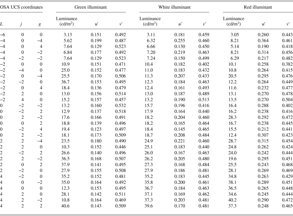
The color chips were selected from the OSA UCS in various lightness levels; L = −6, −4, −2, 0, +2, and +4 in OSA UCS coordinates (MacAdam, Reference MacAdam1974). The chromaticity of each color patch was calculated from the spectral reflectance of the OSA color chip and the illuminant spectrum. Symmetric pairs of colors (j and g for yellow–blue and green–red components, respectively, in OSA UCS coordinates) were chosen with respect to the achromatic point (j = g = 0) to balance the chromaticity. The color patches were also selected such that the chromaticities under the three illuminants remained within the color-rendering area of the CRT display. The Ljg coordinates and CIE u′v′ coordinates under three illuminants for the OSA color chips are listed in Table 1.
OSA UCS and CIE u′v′ coordinates of color chips used in the multicolor surround stimuli
The multicolor surround stimuli were each tiled with simulated OSA color chips, each of which subtended 1.7° × 1.7°. The chips were partially overlapped to fill the surrounding area completely (Fig. 1).
To avoid the accumulation of chromatic adaptation at each retinal location across trials, we prepared 10 different spatial arrangements of the surround stimuli under each illuminant condition, and we presented one of them in each trial. The outer size of the surround color stimulus was 9.7° × 9.7°. A black area (1.9° × 1.9°) appeared in the center for the test stimulus. The mean chromaticities of the surround stimuli under green, white, and red illuminant conditions were (u′, v′) = (0.15, 0.50), (0.19, 0.46), and (0.27, 0.45), respectively. The mean luminance of each multicolor surround stimulus was set to 16 cd/m2 by adjusting the illuminant intensity.
We also used uniform surround stimuli corresponding to the three conditions of green, white, and red illuminants. The chromaticity of each uniform stimulus was adjusted to be identical to the mean chromaticity of the multicolor surround stimulus when simulated under the corresponding illuminant color.
CFS stimuli
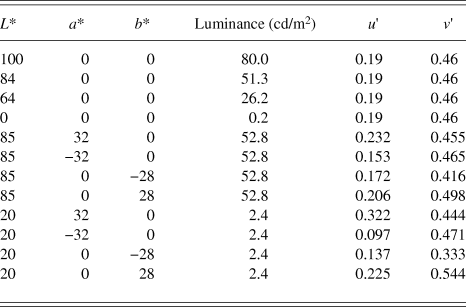
The CFS stimulus was a rapid presentation of a spatially random stimulus at a refresh rate of 14.2 Hz (Tsuchiya & Koch, Reference Tsuchiya and Koch2005). Each CFS frame was created by randomly arranging squares of 12 chromaticities. The chromaticity and luminance of the sets are shown as CIE LAB and u′v′ coordinates in Table 2. They were chosen independent of the element colors for the multicolor surround, but were decided to cover the entire range of luminance and chromaticity of the multicolor surround. Colors for the CFS stimulus were chosen among the 12 colors to contain opponent color pairs, so that the mean chromaticity of each CFS frame was gray. The size of each square was 1.7° × 1.7°, and these were partially overlapped to cover the entire field of the surrounding area, with the exception of the central area. The luminance and chromaticity of each patch were drastically changed (reversed) between the contiguous frames to ensure that luminance and chromatic reversals took place between every frame of the CFS stimulus. The spatial arrangement of the CFS frame changed every other frame to avoid artifacts and aftereffects from the continuous use of identical shapes. The central area, which corresponds to the location of the test color patch and the surrounding gap (1.9° × 1.9°) in the other eye, was colored black (Fig. 1A). The mean chromaticity and mean luminance for each CFS frame were (u′, v′) = (0.19, 0.46) and 16 cd/m2, respectively. The size of each CFS frame was 9.7° × 9.7°.
Chromaticity of patches used in the CFS stimulus
Test stimuli
The size of the test stimulus was 1.7° × 1.7°. We prepared a set of test colors for each subject based on the results of preparatory experiments using 17 test colors with a luminance of either 16 cd/m2 (subjects S1 and S3, the authors) or 21 cd/m2 (naïve subjects S2 and S4–S8). It was easier for naïve subjects to judge unique yellow, i.e., neither reddish nor greenish, by test colors at higher lightness levels than the surrounds. To optimize the range of test stimulus chromaticities used in the staircase procedure to draw psychometric functions, the range of u′ chromaticity was measured in preparation for each subject, such that the range covers whole transitional changes in color appearance from green through yellow to red under all illuminant conditions.
All test colors in the present study were selected on a line in the CIE u′v′ color space that connected a range in the chromaticities of (u′, v′) = (0.17, 0.55) and (0.27, 0.53), each of which corresponds to the chromaticity of a yellowish OSA color chip (L, j, g) = (−2, 6, 0) under the green and red illuminants, respectively. The test stimulus chromaticity varied along a line in the u′v′ chromaticity space as follows:
 $$v\prime = - 0.2u\prime + 0.58\quad .$$
This range was equally divided into 16 intervals (i.e., 17 points, including both ends) to present the same set of 17 test colors in all subjects for the preparatory experiment. The subjective equality of unique yellow was measured with a uniform gray surround using the same procedure as in the main experiment without CFS (i.e., the no-CFS-B condition; see Procedure section for details). After the preparatory experiment, data for each subject were accumulated to derive psychometric curves for each illuminant condition using the Psignifit Toolbox in MATLAB (Wichmann & Hill, Reference Wichmann and Hill2001a,Reference Wichmann and Hillb). The range of test-stimulus chromaticities for the main experiment was determined for each subject, such that the range covers chromaticities that evoke both 0% and 100% red responses under all illuminant conditions. The optimized range of test stimulus chromaticities was sampled at equal intervals in the u′ chromaticity scale to select chromaticities for the test stimulus in the staircase procedure in the main experiment.
Only the u′ chromaticity was used to represent the color of the test stimulus, since its chromaticity co-varied along a line in u′v′ coordinates [eqn. (1)], and the difference in the u′ value is proportional to the Euclidean distance in the u′v′ plane.
Stimulus viewing conditions
Fig. 1A shows a schematic view of the stimuli in the CFS condition. We presented checkerboard frames of 1.2° surrounding the area of the surround stimulus for both eyes to aid with binocular fusion. For all conditions, we presented all stimuli on a gray background (CIE [u′, v′] = [0.19, 0.46], luminance 16 cd/m2).
We employed two conditions of surround stimulus suppression, i.e., CFS and no-CFS. In the CFS condition, we presented the test and surround stimuli to the non-dominant eye and presented the CFS stimulus to the dominant eye (Fig. 1B). To reliably isolate the test stimulus from the perception of the surround stimulus in the non-dominant eye, the test color patch (1.7° × 1.7°) was surrounded by a thin dark gap (0.1°). In addition, a black square (1.9° × 1.9°) was presented on the CFS side at the location corresponding to the test color patch in the other eye.
In the no-CFS condition, there were two viewing settings (Fig. 1B). In one condition, both the test and surround stimuli were presented binocularly (in short, no-CFS-B). To measure the chromatic induction effect without CFS under a nearly natural viewing condition, we employed a binocular viewing condition (in which the same center and surround stimuli were presented), as one of the no-CFS conditions in the main experiment.
However, binocular viewing makes it difficult to reject the possible effects of several binocular-interaction mechanisms under CFS conditions. One example is the binocular mixture of colors (Hovis, Reference Hovis1989) between the surround and the CFS stimulus. If a binocular color mixture occurred, then it would introduce a reduction in the apparent chromatic saturation in the surround stimulus, which in turn could cause a reduction in the chromatic induction. A similar argument can be made for interocular differences in the state of chromatic adaptation, the effects of binocular color mechanisms (Shimono et al., Reference Shimono, Shioiri and Yaguchi2009), and an enhanced neural response (Peirce et al., Reference Peirce, Solomon, Forte and Lennie2008) due to the binocular stimulus presentation. To test these possibilities, we also performed a condition with a monocular presentation of the test and surround stimuli under the no-CFS condition (in short, no-CFS-M) in a slightly modified form, in which an entirely gray uniform field (without the checkerboard frame: Fig. 1B) was presented to the dominant eye to avoid the occurrence of binocular rivalry. The presentation of a black screen or the use of an eye patch yielded frequent binocular rivalry, and it severely interfered with the observer's judgments on the color appearance of the test stimulus. A uniform gray field was presented to prevent dark adaptation in the other eye of the subjects. The uniform gray screen also prevented evoking any transient signal caused by vergence during the experiment.
Procedure
The present study consisted of six conditions (Fig. 1B) and these were tested in separate sessions. Fig. 3 shows the time course for the stimulus presentation in one trial for the CFS condition. The subject initiated a trial by pressing a key (“Press the first key [A]” in Fig. 3A). The CFS stimulus was directly presented at the highest contrast, whereas the contrast of the surrounding stimulus ramped up gradually for 2.0 s to maintain reliable perceptual suppression (Fig. 3B; Hong and Blake, Reference Hong and Blake2009). We presented the test stimulus at the center of the surround stimulus for 0.5 s immediately after the subject pressed the second key (“Press the second key [B]” in Fig. 3A). When perceptual suppression by the CFS was incomplete, the subject perceived “something unchanged” or “something changing slower than the CFS frames” in the surround. The subjects were not allowed to press the second key (key [B]) under such circumstances. Such cases occasionally happened at the end of the session; in most subjects, this was probably due to fatigue during a session. Such a trial was discarded and retested afterward. In the CFS condition, the CFS stimulus was presented for an additional 0.5 s after the disappearance of the surround and test stimuli to block any afterimages that arose as a result of the sudden disappearance of the surround stimulus. The subject was asked to report whether the test stimulus at the center appeared “reddish” or “greenish” (i.e., a two-alternative forced-choice response) by pressing a key after all stimuli disappeared. There was a blank period of 3.0 s between trials to minimize the transfer of chromatic adaptation between trials, and the subject responded during this blank period.
(A) The time sequence for one trial of the CFS condition for the case of a dominant right eye. See Procedure section for details. (B) Time sequence for the contrast of the test and surround stimuli during one trial. The solid black line denotes the contrast of the surround stimulus. The solid red line denotes the contrast of the test stimulus.
The chromaticity of the test stimulus in the next trial was determined by the staircase procedure (1-up, 1-down) within the set of test colors defined for each subject in the preparatory experiment. Each session of the main experiment included three illuminant conditions, and each illuminant condition was conducted as a separate staircase trial. Both ascending and descending series were conducted in a session. A session consisted of six staircases (two staircases each for the three illuminant conditions), and all staircase series were randomly interleaved within a session. Each staircase was terminated after ten reversals of the staircase directions. The total number of trials was around 180–200 in each session.
Analysis
The data collected for each illuminant and viewing condition were plotted as a psychometric function by calculating the percentage of “reddish” responses and plotting this as a function of the u′ chromaticity of the test-stimulus. The results of the ascending and descending series of staircase experiments were summarized for each viewing condition to draw a psychometric function. Each psychometric function was then fitted with a cumulative Gaussian function using the Psignifit Toolbox (Wichmann & Hill, Reference Wichmann and Hill2001a,Reference Wichmann and Hillb) for MATLAB to obtain the u′ value corresponding to the point of subjective equality (PSE) with unique yellow (i.e., neither reddish nor greenish) and a 95% confidence interval. We defined the difference in u′ values for PSEs under red and green illuminant conditions (Δu′) as the magnitude of the color shifts induced under a surround stimulus condition.
The general methods for statistical analysis of the main experiment were as follows. First, a significant difference of the chromatic induction effect from zero was tested by a one-sample, two-tailed t-test. Second, a within-subject analysis of variance (ANOVA) was applied to test statistically significant differences between the experimental factors. A post hoc analysis with Tukey's test was also applied to compare statistically significant differences between experimental conditions, when necessary.
Subjects
Two of the authors (S1 and S3) and six naïve subjects participated in the experiment. All subjects had normal or corrected-to-normal visual acuity. All subjects were confirmed to have normal color vision by using Ishihara pseudo-isochromatic plates (Ishihara, Reference Ishihara1996). The experimental methods were approved by the ethics committee of the Research Institute of Electrical Communication, Tohoku University, according to the guidelines based on the Declaration of Helsinki.
Results
Confirmation of CFS effect
To verify the consistency of perceptual suppression with the CFS stimulus, we conducted a session to confirm perceptual suppression in each subject. The subjects were asked to report the color of an illuminant condition in the multicolor surround stimulus presented to the non-dominant eye, while the CFS stimulus was presented to the dominant eye. Interocular suppression tends to fail when a transient signal (such as an eye blink, small saccades, and so on) is detected in the other eye of the suppression stimulus (Blake and Logothetis, Reference Blake and Logothetis2002; Hong and Blake, Reference Hong and Blake2009). Since the multicolor surround stimulus consisted of sharp luminance edges, the detectability for the failure of interocular suppression was higher.
The experimental procedure was the same as for the main experiment. If perceptual suppression was successful, then the hit rate is expected to be at the level of random chance (50%). All eight subjects participated in this session (with 180 trials per subject).
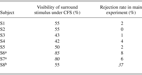
As shown in Table 3, two naïve subjects (S6 and S7) showed high hit rates of above 80%, which implies the possibility of incomplete suppression by CFS during the main experiment. In addition, the rejection rates for S6 and S7 are relatively higher than those for S1–S5. In addition, subject S8 showed an extremely high rejection ratio for 37% of trials in the main experiment. It is theoretically possible to accept results of non-rejected trials. However, compared with the average rejection rate of 4% in other subjects, the rejection ratio of 37% is extremely high. It is natural to consider that something occurred in S8 that was different from the other subjects. Thus, only data for subjects S1–S5 were used in the main results in the following.
The percentage correct for the confirmation experiment and the rejection rate in the main experiment
a Data not analyzed in main experiment due to high visibility of surround stimulus under interocular suppression.
b Data not analyzed in main experiment due to extremely high rejection rate.
Main results
Fig. 4A shows a typical psychometric function obtained for subject S1 based on color-appearance judgments for the test stimuli under the no-CFS condition with the multicolor surround stimulus.
(A) Psychometric functions from a representative subject (S1) and an example of the color-shift effect of the surround stimulus colors. Each psychometric function corresponds to the judgment of a color appearance of the test stimulus for an illuminant-color condition under the no-CFS condition with the multicolor surround stimulus. The horizontal error bars on the fitted psychometric functions represent 95% confidence intervals at 20, 50, and 80 percentile points derived by a bootstrap procedure using the Psignifit Toolbox (Wichmann & Hill, Reference Wichmann and Hill2001a,Reference Wichmann and Hillb) on MATLAB. (B) Left and right panels show 50 percentile points in panel A for all subjects under multicolor- and uniform-surround conditions, respectively. The vertical axis indicates the u′ coordinate of the PSE to unique yellow. Different symbols indicate different illuminant conditions: square, circle, and triangle symbols indicate red, white, and green illuminant conditions, respectively. Three symbols on the left, center, and right in each subject indicate results under no-CFS-M, no-CFS-B, and CFS conditions, respectively. Error bars indicate 95% confidence intervals.
Fig. 4B shows the shifts in the u′ coordinate for the PSE for unique yellow, i.e., the 50 percentile points and corresponding 95% confidence intervals for each illuminant condition. As expected, the PSEs for unique yellow shifted toward the illuminant color. The PSEs under reddish and greenish illuminant conditions shifted slightly toward the reddish direction (positive along the vertical axis) and the greenish direction (negative), respectively, compared with the PSE under the white illuminant condition. Overall, the shifts between white- and green-illuminant conditions were smaller than those between white- and red-illuminant conditions. This may primarily be due to the difference in mean chromaticity shifts from the white illuminant condition, especially in the direction along the u′ coordinate.
In the following, the effect of color shifts from the surround stimuli will be described by the magnitude of the color shifts (Δu′) defined by differences in the u′ values at 50 percentile points for the results under red and green illuminant conditions, i.e., the distance between symbols for red- and green-illuminant conditions in Fig. 4B. The positive sign of the chromatic induction effect indicates shifts in the PSEs of unique yellow toward the illuminant colors, and the negative sign indicates shifts in the opposite direction.
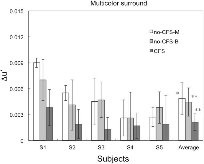
Fig. 5 shows the magnitude of Δu′ for each subject in the multicolor surround condition. To test the statistical significance of the chromatic induction effect, we applied a one-sample, two-tailed t-test against zero as an a priori test. In the no-CFS condition, significant color shifts were observed for all subjects under monocular (t(4) = 4.38, P < 0.05) and binocular (t(4) = 6.02, P < 0.005) presentation conditions. In the CFS condition, the average magnitude of the color shifts across all subjects was significantly greater than zero (t(4) = 5.01, P < 0.01).
The results for the two CFS conditions with the multicolor surround stimulus, which show the magnitude of color shifts between the red and green illuminant-color conditions for each subject. The white, medium gray, and dark gray bars show the results for the no-CFS-M, no-CFS-B, and CFS conditions, respectively. The rightmost bars show the average Δu′ across all subjects. The error bars for each subject denote the estimated 95% confidence intervals, and the error bars for the average across all subjects represent the SEM. Asterisks (* and **) indicate statistical significance after the Bonferroni correction (*: P < 0.00833; **: P < 0.00167 with the two-tailed t-test). See Main Results section for details.
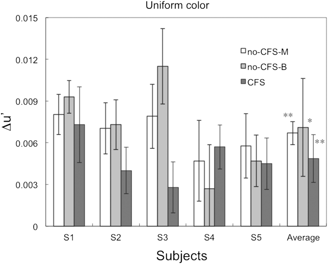
Fig. 6 shows the magnitude of color shifts (Δu′) for each subject in the uniform surround stimulus condition. In the a priori test (one-sample, two-tailed t-tests against zero) under the no-CFS condition, the average color shifts across all subjects were statistically significant under monocular presentation (t(4) = 9.35, P < 0.0005) and binocular presentation (t(4) = 4.70, P < 0.05) conditions. Similarly, under the CFS condition, the average magnitude of color shifts across all subjects was significantly greater than zero (t(4) = 6.20, P < 0.005).
The results for the uniform surround stimulus condition, showing the magnitude of color shifts among the red and green illuminant-color conditions for each subject. The rightmost bars show the average color shift across all subjects. The bar colors, asterisks, and error bars represent the same parameters and values as those in Fig. 5. The error bars for each subject denote the estimated 95% confidence intervals, and the error bars for the average across all subjects represent the SEM.
The statistical tests on the color-induction effects averaged across subjects under each surround and viewing condition in Figs. 5 and 6 exhibited significant differences from zero, even after a Bonferroni correction for the multiple comparisons, except that the no-CFS-M condition with multicolor surround and the no-CFS-B condition with uniform surround were marginally significant. This result implies that there were statistically significant color shifts due to changes in the surround color, even when the surround stimulus was perceptually suppressed by the CFS stimulus. This is one of the most important findings of the present study.
To compare statistically significant differences among experimental conditions, a two-factor within-subject ANOVA was applied by taking the surround stimulus (multicolor or uniform) and the viewing conditions (no-CFS-M, no-CFS-B, or CFS) as the factors. There is a significant effect from the surround stimulus (F(1,4) = 38.3, P < 0.01) and viewing conditions (F(2,8) = 4.72, P < 0.05), but no significant interaction was detected (F(2,8) = 0.293, n.s.). Since the number of subjects was small, the Greenhouse–Geisser (G-G) and Huynh–Feld (H-F) methods were also applied to correct for the sphericity assumption in the ANOVA. As a result, the effect of the surround stimulus was significant (P < 0.005 for G-G; P < 0.005 for H-F) and the effect of viewing conditions was marginally significant (P = 0.0869 for G-G; P = 0.0783 for H-F). According to a t-test analysis on the effects of viewing condition, the average color shifts in the CFS condition were significantly different from those in the no-CFS-M (t(9) = 3.53; P < 0.05), but not between other pairs (no-CFS-B vs. CFS: t(9) = 2.43; no-CFS-B vs. no-CFS-M: t(9) = 0.011; both n.s.). The significant difference between the no-CFS-M and CFS conditions (regardless of the surround conditions) in this statistical test indicates that the possible artifacts of the various binocular effects (described in Methods section) are not the primary cause of the reduction in the color shifts under the CFS condition.
Another t-test analysis on the effect of the surround conditions showed that the average color shift in the multicolor surround was significantly smaller than the color shifts with the uniform-colored surround (t(14) = 5.16, P < 0.01). This is analogous to previous reports (Brown & MacLeod, Reference Brown and MacLeod1997; Brenner et al., Reference Brenner, Ruiz, Herráiz, Cornelissen and Smeets2003), in which the magnitude of chromatic induction was smaller for the surround with additional chromatic modulation than with a uniform surround.
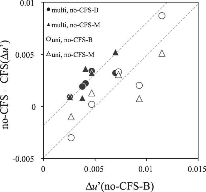
In Fig. 7, the effects of CFS for the two surround conditions and two viewing conditions are plotted against the size of chromatic induction under no-CFS-B conditions (i.e., under the most natural viewing conditions) for each subject.
Comparison of CFS effects between conditions. The vertical axis represents the difference in color shifts (Δu′) between the no-CFS and CFS conditions under each surround condition. The horizontal axis represents the color shifts under no-CFS-B conditions. Each symbol represents the results for each subject, and different symbols represent differences in viewing and surround conditions; circle and triangle symbols represent no-CFS-B and no-CFS-M conditions, respectively, and open and filled symbols represent uniform and multicolor surround conditions, respectively. Thin lines show the results of linear fits to the two conditions with a common slope (a Type III model). See the Appendix B for details of fittings.
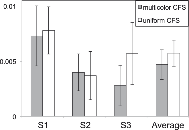
Comparison of the effects of multicolor and uniform CFS stimuli. The shaded bars on the left and open bars on the right represent the results for multicolor and uniform CFS, respectively. The results of the multicolor CFS are the same as those in Fig. 5. The error bars for each subject denote the estimated 95% confidence intervals, and the error bars for the average across all subjects represent the SEM.
The effect of CFS in each subject appears to be proportional to the original effect of chromatic induction under the most natural viewing conditions, and the slopes of the fitted lines to the results under the two surrounds appear similar. This implies that mechanisms for the CFS effect are common under both surrounds, which supports the results of the ANOVA. See Appendix B for the details of the model fittings.
Effects of spatial frequency component differences
We attributed differences between the effects of the CFS with the multicolor and uniform color conditions to different contributions of mechanisms for integrating spatially distributed colors. An alternative explanation may be that the differences in the effects of the CFS on the multicolor and uniform surrounds are caused by differences in the spatial frequency characteristics of the surrounds and the CFS stimuli. The spatial structure of each frame of the CFS was very similar to that of the multicolor surround stimulus, but not to that of the uniform surround stimulus (Hong & Blake, Reference Hong and Blake2009).
To test this possibility, we conducted a supplemental experiment with a uniform CFS stimulus and a uniform surround stimulus. If the spatial structure of the CFS stimulus was irrelevant to the spatial structure of the surround stimuli, then the results would not differ from those of the main experiment. The uniform CFS stimulus consisted of uniform frames that rapidly alternated between 12 colors at a temporal frequency of 14.2 Hz, each of which was used to form the CFS frames in the main experiment.
The results were similar to those of the main experiment for the multicolor CFS condition with the uniform surround stimulus. The color shifts were measured for three subjects who participated in the main experiment (S1, S2, and S3). Results of all subjects and the average is shown in Figure 8. The averaged results for the two experiments were 0.0047 ± 0.0013 (mean ± the standard error of the mean (SEM)) and 0.0057 ± 0.0012 for the multicolor CFS and uniform CFS conditions, respectively. Therefore, the spatial structure of the CFS stimulus is not a major contributor to the smaller reductions in the surround chromatic induction under the uniform surround condition.
Discussions
Summary of the results
The main finding of our results is the presence of chromatic induction effects under the perceptual suppression of surround stimuli by the CFS stimulus (Figs. 5 and 6). This implies the presence of at least one mechanism for the chromatic induction effect, which still operates under interocular suppression.
We used a CFS stimulus (Tsuchiya and Koch, Reference Tsuchiya and Koch2005) that changed in color and luminance randomly at a high spatiotemporal frequency. Color perception from the stimulus in the other eye was blocked at the retinal location corresponding to the CFS with a high probability (Table 3). Previous studies on the efficiency of interocular suppression in relation to the magno- and parvo-cellular pathways have shown that the means of interocular interactions are different between the two pathways. One psychophysical study showed that the use of isoluminant CFS did not suppress motion-direction perception of the Gabor pattern that was defined by both color and luminance, while color discrimination was significantly impaired. This study also reported that monochromatic CFS suppressed form (orientation) perception, but yielded “a formless cloud of color” perception at the same time (Hong and Blake, Reference Hong and Blake2009). Another psychophysical study on interocular suppression reported that perceived color was never combined (i.e., rivalry), but that the perceived flicker frequency was a nonlinear combination of both eyes' stimuli, when they differed in color, flicker frequency, and shape (Carlson and He, Reference Carlson and He2000). Both studies suggested that the signal predominantly conveyed through the parvocellular pathway was blocked by color in the other eye, but not by monochromatic stimulus alone. Our results, obtained under the use of CFS stimulus with such characteristics, suggest that the chromatic induction from surrounding color stimuli is built up through mechanisms that reside at both levels before and after the site of interocular suppression.
The statistically significant difference between multicolor and uniform surrounds indicates that the efficiency of chromatic induction is higher with a uniform surround than a multicolor surround, even when the mean chromaticities are nearly equal. This is consistent with previous studies (Brown & MacLeod, Reference Brown and MacLeod1997; Brenner et al., Reference Brenner, Ruiz, Herráiz, Cornelissen and Smeets2003). However, contrary to our expectation, the difference between the two surround stimuli did not affect the strength of CFS. The effect of surround stimulus conditions will be discussed in the next section.
Effect of surround stimulus
In comparison with studies of color constancy in which the articulated surround improved the degree of color constancy (i.e., larger chromatic shifts) (Kuriki & Uchikawa, Reference Kuriki and Uchikawa1996; Linnell and Foster, Reference Linnell and Foster2002), it is somewhat counterintuitive that our results showed smaller color shifts in the presence of a multicolor surround, which faithfully simulated the real object surfaces under chromatic illuminants. The aim of using two surround stimuli was to find some differences in the magnitude of the CFS effect on the chromatic induction. This was based on an assumption that the chromatic induction from a uniform surround may originate more from monocular and/or lower-level mechanisms (Brenner and Cornelissen, Reference Brenner and Cornelissen1991; Chichilnisky and Wandell, Reference Chichilnisky and Wandell1995), compared with that from the multicolor surround (Goltz & MacLeod, Reference Goltz and MacLeod2002), and thus the reduction of chromatic induction by the CFS is smaller than the multicolor-surround condition. Nevertheless, our stimulus had a large gray uniform field outside the frame of the colored surround stimuli, which was presented to prevent the subjects' visual systems from dark adaptation, and it was not obvious for the subjects to interpret the inside of the frame as another illuminated environment. This condition is different from the stimuli present in typical studies of color constancy. Our multicolor surround probably did not effectively activate the mechanisms that calculate color-luminance statistics such as correlations.
Conversely, it has also been reported that the higher variability in surround colors reduces the perceived saturation in the center (Brown and MacLeod, Reference Brown and MacLeod1997). This high variability may be one factor for the reduction in color shifts in the multicolor surrounds. The difference in the efficiency of the chromatic induction between the uniform and multicolor surrounds can also be explained by assuming a chromatic induction mechanism in which the consistency of local chromatic contrast along the edge of the test stimulus is the determining factor (Land & McCann, Reference Land and McCann1971; Brenner et al., Reference Brenner, Ruiz, Herráiz, Cornelissen and Smeets2003).
The similar amount of reduction in chromatic induction by the CFS for the two surround conditions implies that the processing of color appearance, which enabled subjects to judge unique yellow under chromatic induction from the chromatic surrounds, shares common subsystems at a level higher than that of the interocular suppression. Since interocular suppression is thought to occur no earlier than the cortical level (Blake and Logothetis, Reference Blake and Logothetis2002; Watanabe et al., Reference Watanabe, Cheng, Murayama, Ueno, Asamizuya, Tanaka and Logothetis2011), it is possible that these subsystems reside later than the cortical level and that they also operate under chromatic induction from the uniform surround stimulus. This is consistent with previous studies that reported the presence of cortical neurons that exhibit the opponent color induction from uniform surrounds (Schein and Desimone, Reference Schein and Desimone1990; Wachtler et al., Reference Wachtler, Sejnowski and Albright2003). Furthermore, considering the study by Land et al. (Reference Land, Hubel, Livingstone, Perry and Burns1983), cortical mechanisms may also play a role in the establishment of color appearance for unique yellow in the stimulus surrounded by the colored area, in addition to the lower-level mechanisms with classical receptive fields with spatiochromatic (i.e., double) opponency.
Hence, our results suggest that the overall color-induction effect is achieved as a summation of color-induction effects from at least two mechanisms. The first mechanism, which is unaffected by the CFS and probably resides in lower level than the interocular suppression, yields a different color-induction effect from uniform and multicolor surrounds. This mechanism may process information from a relatively small area in the visual field whose total effect can be affected by the consistency of local chromatic contrast along the edge (Brown & MacLeod, Reference Brown and MacLeod1997; Brenner et al., Reference Brenner, Ruiz, Herráiz, Cornelissen and Smeets2003). The second mechanism resides in a higher level than the interocular suppression, and the chromatic induction effect is affected by the CFS as a change in its gain.
The relative efficiency of the interocular suppression by the CFS was different between the multicolor and uniform surrounds, when evaluated by the chromatic induction under CFS normalized to that under no-CFS-B. The relative reductions with the multicolor CFS were larger for the multicolor surround: 0.487 ± 0.138 (mean ± SEM) and 0.940 ± 0.355 for multicolor and uniform surrounds, respectively [N = 5; t(4) = 3.40, P < 0.05]. The relative efficiency was similar on a uniform surround, when compared between the multicolor and uniform CFSs: 0.745 ± 0.093 (mean ± SEM) and 0.739 ± 0.129 for multicolor and uniform CFSs, respectively (N = 3). This relative-efficiency analysis confirmed our hypothesis on the two subsystems for the chromatic induction, because the results are consistent with the tendency found in the main results (Figs. 5, 6, and 7), which is as follows: the difference in chromatic induction from the complexity of the surround stimulus was not severely affected by the CFS, and the relative contribution of such lower-level mechanisms to chromatic induction from the multicolor surround was smaller than that from the uniform surround.
It is difficult to specify the exact sites corresponding to the difference in the surround condition and the reduction due to the CFS effect, because the mechanisms and sites for interocular suppression remain unknown (Lumer et al., Reference Lumer, Friston and Rees1998; Blake & Logothetis, Reference Blake and Logothetis2002; Tong et al., Reference Tong, Meng and Blake2006). These issues should be investigated in future studies.
Relations with binocular interaction and chromatic adaptation mechanisms
Owing to the significant difference between the no-CFS-M and CFS conditions detected in the post hoc analysis of the ANOVA shown in the main results (Figs. 5 and 6), it is possible that the effect of the CFS stimulus was not simply due to the binocular mixture of chromatic (multicolor surrounds) and achromatic (CFS) mean colors in the surrounding area (Hovis, Reference Hovis1989), interocular differences in the state of chromatic adaptation, any effects of binocular color mechanisms (Shimono et al., Reference Shimono, Shioiri and Yaguchi2009), or the enhancement of neural response due to binocular stimulation (Peirce et al., Reference Peirce, Solomon, Forte and Lennie2008).
If any interocular difference in the state of chromatic adaptation caused changes in the color appearance of the test stimulus, then it could cause a reduction of chromatic induction in the CFS condition. In several previous studies on color appearance under different illuminant colors, asymmetric chromatic adaptation between the eyes was used in the studies on corresponding color surfaces under different illuminants, and the state of chromatic adaptation of each of the eyes was considered to be almost independent (Chichilnisky & Wandell, Reference Chichilnisky and Wandell1995; Kuriki et al., Reference Kuriki, Oguma and Uchikawa2000; Fairchild, Reference Fairchild2005). Given that photoreceptor level–adaptation occurred for a short duration, the effect is common between the no-CFS-M and CFS conditions. It is also known that it takes several tens of seconds before the chromatic adaptation affects the judgment of color appearance (Fairchild and Reniff, 1995; Kuriki and MacLeod, Reference Kuriki, MacLeod, Dickinson, Murray and Carden1998; Shevell, Reference Shevell2000). Meanwhile, the surround stimulus in our experiment was presented only for five seconds and the contrast of the surrounds was ramped up gradually, taking 3.5 s to reach its maximum. Accordingly, regardless of the state of interocular suppression, it is difficult to consider that the chromatic adaptation mechanisms play a significant role in shifts in color appearance for the test stimulus presented in the chromatic surrounds. Therefore, we consider that the differences in chromatic adaptation cannot be the primary factor that caused changes in color appearance between conditions with and without interocular suppression in the present study.
A previous study on a subject with corpus callosum dissection reported that color constancy did not hold when the surround stimuli were presented in the non-perceptible side of the subject (Land et al., Reference Land, Hubel, Livingstone, Perry and Burns1983). This study suggested that the presence of pictorial information on the retina alone is insufficient for color constancy. Our method of study may serve as an analog to this patient study (Land et al., Reference Land, Hubel, Livingstone, Perry and Burns1983) in healthy subjects with the aid of the CFS stimulus.
Acknowledgment
The authors thank the subjects who participated in this study. The authors also thank the two anonymous reviewers for their constructive comments and helpful discussions. This study was supported by a Grant-in-Aid for Scientific Studies (Kakenhi #22243044 and #24330205 to IK) from the Japan Society for the Promotion of Science.
Appendix A
Method and parameters of calibration of the computer screen
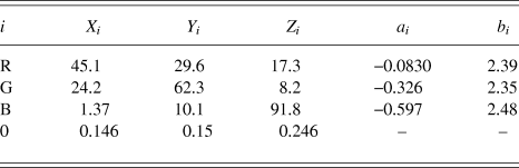
All photometric measurements were conducted with a spectroradiometer SR-UL1R (Topcon, Japan), which is designed to measure luminance around 0.01 cd/m2. The CIE XYZ tristimulus values of three color primaries (red, green, and blue; in short, R, G, and B) are as shown in Table A1.
Parameters for CRT monitor calibration

The tristimulus value for a light rendered with the given relative intensities of the three color primaries can be described as follows:
 $$\left[ {\matrix{ {X_{\rm{c}} } \cr {Y_{\rm{c}} } \cr {Z_{\rm{c}} } \cr } } \right] = \left[ {\matrix{ {X_{\rm{R}} } &amp; {X_{\rm{G}} } &amp; {X_{\rm{B}} } \cr {Y_{\rm{R}} } &amp; {Y_{\rm{G}} } &amp; {Y_{\rm{B}} } \cr {Z_{\rm{R}} } &amp; {Z_{\rm{G}} } &amp; {Z_{\rm{B}} } \cr } } \right]\left[ {\matrix{ {rL_{\rm{R}} } \cr {rL_{\rm{G}} } \cr {rL_{\rm{B}} } \cr } } \right] + \left[ {\matrix{ {X_0 } \cr {Y_0 } \cr {Z_0 } \cr } } \right]\quad ,$$
where [X i, Y i, Z i] represent tristimulus values for color primaries (when i = R, G, or B) for a resultant color (i = c), or they represent zero digital values for all color primaries (i = 0). The term rL i represents the relative luminance of each color primary (i = R, G, or B) normalized to the maximum intensity of the corresponding color primary.
The luminances of each color primary for given digital values were measured using the spectroradiometer, and were fitted with a second-order polynomial in a log–log space, after normalizing to its maximum (Cowan, Reference Cowan1983). Formulation is as follows:
 $${\log _{10}}\left( {r{L_i}} \right) = {a_x}{\left( {{{\log }_{10}}\left( {{{{D_i}} \mathord{\left/ {\vphantom {{{D_i}} {{D_{i{\rm{MAX}}}}}}} \right. \kern-\nulldelimiterspace} {{D_{i{\rm{MAX}}}}}}} \right)} \right)^2} + {b_i}\left( {{{\log }_{10}}\left( {{{{D_i}} \mathord{\left/ {\vphantom {{{D_i}} {{D_{i{\rm{MAX}}}}}}} \right. \kern-\nulldelimiterspace} {{D_{i{\rm{MAX}}}}}}} \right)} \right)\quad ,$$
where D i and the D iMAX represent a digital value and the highest digital value of a color primary (i = R, G, or B), respectively, and a i and b i represent the coefficients for the second- and first-order terms, respectively. The coefficients a i and b i were obtained for each color primary i by fitting this function to the results of photometric measurements using the method of least squared error. To render the highest luminance of a color primary i with the maximum digital value D iMAX, the constant term was fixed to zero. Note that [X 0; Y 0; Z 0] was subtracted from all tristimulus values before this fitting. All values of a i and b i (i = R, G, or B) used in this study are shown in Table A1.
To derive the chromaticity of a given triplet of digital values (D R, D G, D B), they were first transformed to the relative luminance of each color primary normalized to its maximum (i.e., rL i) with eqn. A2. A look-up table was generated with this procedure to find the luminance for each digital value. Then, eqn. A1 was used to derive the tristimulus values of all color primaries. To render a color with the designated tristimulus values, the inverse calculations of this process can be conducted to obtain the triplet of digital values.
Appendix B
Linear model fittings and evaluation
The ANOVA in the main results revealed significant main effects, but the interaction was not significant (see Main Results section for details). However, non-significance itself does not mean non-different; it simply could not detect significant differences between conditions. Therefore, we applied another method of analysis to confirm the non-difference further by fitting linear models to the data plotted in Fig. 7.
We then used the linear model fittings to investigate the relationships between the effect of CFS and the magnitude of chromatic induction by calculating the effect of CFS within each subject under each surround condition, defined by the difference in color shifts (Δu′) between the no-CFS-B and CFS conditions, and between the no-CFS-M and CFS conditions. The formulation of the fitted linear models is as follows:
 $${\rm{CFSeffect}}{\__i} = {\rm{slope}}{\__i} \times {\rm{colorshift}}{\__i} + {\rm{intercept}}{\__i}\quad ,$$
where subscript i represents the difference in surround stimulus, when applicable; CFSeffect and colorshift represent the effect of CFS and the chromatic induction effect under the no-CFS-B condition, respectively.
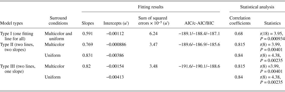
We used three types of models. The Type I model uses one slope and one intercept for all surround conditions; i.e., differences in the surrounds were ignored. The Type II model employs two slopes and two intercepts; i.e., one slope and intercept for each surround condition. The Type III model employs one common slope for the two surround conditions, and two intercepts for different surround conditions. The model parameters were optimized to obtain the least mean squared errors. The detailed parameters and statistics are summarized in Table A2.
Parameters of the model fittings in Fig. 7
Although the Type II model exhibited the smallest error from the data, the size of the error is only slightly different from that of the Type III model. Furthermore, the Type II model employed the largest number of parameters for the fitting. Therefore, we used indices that penalize the number of fitting parameters of numerical models, such as the Akaike's Information Criterion (AIC) (Akaike, Reference Akaike1974), corrected AIC (c-AIC) (Hurvich & Tsai, Reference Hurvich and Tsai1989), and the Bayesian Information Criterion (Schwarz, Reference Schwarz1978) measures to take the over-fitting problem into consideration. Finally, the indices for the Type III model (one slope, two intercepts) were all had the smallest values (Table A2), which implies that the Type III model is the most efficient.
The use of a common slope model enabled a statistical evaluation of the data distribution in the perpendicular direction of the fitting lines. When data in Fig. 7 are orthogonally projected onto a line perpendicular to the fitted lines, the distribution of the points along the line yields two clusters with significantly different means after a two-tailed t-test (t(9) = 5.12; P < 0.005).
The slope in the model represents the gain of the CFS effect, while the intercept represents the magnitude of chromatic induction under the no-CFS conditions when transposed to the horizontal shifts. Therefore, these results may strongly support the non-difference of the CFS effects between surrounds. This analysis of the models also implies the possible presence of common mechanisms of interocular suppression for the two surround conditions.