


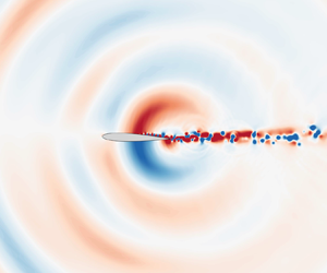




1. Introduction
An aerofoil in freestream can radiate strong, narrow-band pressure waves from the trailing edge. This pressure wave radiation, known as trailing-edge noise, arises from an acoustic feedback between the trailing edge and the boundary layer over the mid-chord (Desquesnes, Terracol & Sagaut Reference Desquesnes, Terracol and Sagaut2007; Fosas de Pando, Schmid & Sipp Reference Fosas de Pando, Schmid and Sipp2014). Trailing-edge noise appears in low-speed flows over a range of moderate Reynolds numbers, and the peak loudness can reach over 40 dB above the background level (Nash, Lowson & McAlpine Reference Nash, Lowson and McAlpine1999; Nakano, Fujisawa & Lee Reference Nakano, Fujisawa and Lee2006). With the recent trend of downsizing aircraft, including unmanned air vehicles and air taxis, noise reduction is a critical component of design for the aforementioned flow conditions (Taira & Colonius Reference Taira and Colonius2009; Ananda, Sukumar & Selig Reference Ananda, Sukumar and Selig2015). Understanding the physical mechanism of trailing-edge noise could facilitate achieving the noise reduction of small-scale aircraft and other aerodynamic machinery.
Since the early 1970s, many studies have been undertaken from theoretical (Fink Reference Fink1975; Howe Reference Howe1978; Kingan & Pearse Reference Kingan and Pearse2009; Ricciardi, Arias-Ramirez & Wolf Reference Ricciardi, Arias-Ramirez and Wolf2020), experimental (Paterson et al. Reference Paterson, Vogt, Fink and Munch1973; Arbey & Bataille Reference Arbey and Bataille1983; Lowson, Fiddes & Nash Reference Lowson, Fiddes and Nash1994; Nash et al. Reference Nash, Lowson and McAlpine1999; Moreau & Roger Reference Moreau and Roger2005; Nakano et al. Reference Nakano, Fujisawa and Lee2006; Pröbsting & Yarusevych Reference Pröbsting and Yarusevych2015; Noda et al. Reference Noda, Nakakita, Wakahara and Kameda2018) and numerical (Desquesnes et al. Reference Desquesnes, Terracol and Sagaut2007; Kurotaki et al. Reference Kurotaki, Sumi, Atobe and Hiyama2008; Le Garrec, Gloerfelt & Corre Reference Le Garrec, Gloerfelt and Corre2008; Sandberg et al. Reference Sandberg, Jones, Sandham and Joseph2009; Tam & Ju Reference Tam and Ju2012; Fosas de Pando et al. Reference Fosas de Pando, Schmid and Sipp2014; Fosas de Pando, Schmid & Sipp Reference Fosas de Pando, Schmid and Sipp2017) perspectives to improve the understanding of trailing-edge noise generation. Paterson et al. (Reference Paterson, Vogt, Fink and Munch1973) conducted pioneering trailing-edge noise experiments with two-dimensional NACA aerofoils at various angles of attack and Reynolds numbers in an open-jet wind tunnel. Their results identified flow conditions at which intense noise radiations occur. The broad consensus in previous studies is that acoustic feedback plays an essential role in sustaining the trailing-edge noise. Arbey & Bataille (Reference Arbey and Bataille1983) suggested that acoustic feedback is established between the trailing edge and the boundary layer over the aerofoil. A detailed analysis of the hydrodynamic instabilities of the boundary layer was performed by Nash et al. (Reference Nash, Lowson and McAlpine1999) by employing a high-resolution laser-Doppler anemometer measurement. Their experimental results indicate that the velocity fluctuations are strongly amplified inside the laminar separation bubble on the pressure side. They also performed a hydrodynamic instability analysis by considering the Orr–Sommerfeld equation. Their result shows that the most amplified frequency of the Tollmien–Schlichting waves agrees with the dominant frequency of trailing-edge noise. The strong fluctuations on the pressure side are also identified experimentally by using particle image velocimetry (Nakano et al. Reference Nakano, Fujisawa and Lee2006; Pröbsting & Yarusevych Reference Pröbsting and Yarusevych2015) and pressure-sensitive paint (Noda et al. Reference Noda, Nakakita, Wakahara and Kameda2018) measurements.
Numerical studies reported in-depth insights from a full acoustic feedback analysis. Desquesnes et al. (Reference Desquesnes, Terracol and Sagaut2007) presented a model of the trailing-edge noise for the dominant tonal noise. Their linear stability analysis via the Chebyshev collocation method shows that the laminar separation bubble on the pressure side is crucial in amplifying the velocity fluctuations and in selecting the dominant frequency. Their local linear stability analysis suggests that the hydrodynamic instabilities may be essential in selecting the dominant frequency. However, a complete understanding of the trailing-edge noise generation mechanism cannot be achieved solely by such linear stability analysis since it depends on a local-parallel flow assumption. To this end, the last two decades of progress on global stability analysis (Theofilis Reference Theofilis2003, Reference Theofilis2011) have advanced our understanding of the feedback loop coupled with boundary layer instability and reception of the acoustic disturbances. Fosas de Pando et al. (Reference Fosas de Pando, Schmid and Sipp2014) performed a global stability analysis of trailing-edge noise flow and suggested that the acoustic feedback mechanism of the dominant tonal noise is related to the least stable modes. Moreover, the same authors employed an adjoint (Fosas de Pando et al. Reference Fosas de Pando, Schmid and Sipp2017) and resolvent analysis for receptivity analysis (Fosas de Pando, Schmid & Sipp Reference Fosas de Pando, Schmid and Sipp2013; Fosas de Pando & Schmid Reference Fosas de Pando and Schmid2014) and showed that the predominant tonal noise originates from the instability on the pressure-side of the aerofoil. More recently, Ricciardi, Wolf & Taira (Reference Ricciardi, Wolf and Taira2022) employed bi-global stability and resolvent analysis to understand the role of flow instabilities on multiple secondary tones around a main tone frequency. They argued that a laminar separation bubble on the suction side of the aerofoil acts as an amplifier and leads to vortex shedding on the suction side.
Previous studies have elucidated the mechanism of the main tone of trailing-edge noise, but have not focused on higher-frequency secondary tones (Oberai, Roknaldin & Hughes Reference Oberai, Roknaldin and Hughes2002; Wolf, Azevedo & Lele Reference Wolf, Azevedo and Lele2012). The higher-frequency tones have different physical features from the main tonal noise. The higher-frequency tone has a quadrupole sound source, while the main tonal noise is widely considered to have a dipole source. The difference in sound source indicates that the acoustic pressure direction has frequency dependency, which makes the trailing-edge noise phenomena more complicated. Previous studies suggested that the quadrupole source originated from a three-dimensional turbulent flow over an aerofoil (Oberai et al. Reference Oberai, Roknaldin and Hughes2002; Khalighi et al. Reference Khalighi, Mani, Ham and Moin2010). However, some signatures of high-frequency sound features can be found in an acoustic spectrum of a numerical simulation (Desquesnes et al. Reference Desquesnes, Terracol and Sagaut2007) and global stability analysis (Fosas de Pando et al. Reference Fosas de Pando, Schmid and Sipp2014), even for a two-dimensional set-up. These results have high-frequency acoustic features, but evidence of quadrupole sound is not clear. Wolf et al. (Reference Wolf, Azevedo and Lele2012) argued that the acoustic direction of the higher-frequency tone is sensitive to the uniform flow conditions. Despite the previous studies' clarification of the basic characteristics of the higher-frequency tone, its physical mechanism and origin remain undiscovered.
In order to understand the origin of the multi-component tones, we apply modal analysis techniques (Taira et al. Reference Taira, Brunton, Dawson, Rowley, Colonius, McKeon, Schmidt, Gordeyev, Theofilis and Ukeiley2017, Reference Taira, Hemati, Brunton, Sun, Duraisamy, Bagheri, Dawson and Yeh2020) on the flow field around an aerofoil where trailing-edge noise is generated. First, we perform dynamic mode decomposition (DMD) (Schmid Reference Schmid2010) on the flow field to extract the dominant coherent flow structures. We then employ resolvent analysis with respect to the linearized governing equations (Trefethen et al. Reference Trefethen, Trefethen, Reddy and Driscoll1993; McKeon & Sharma Reference McKeon and Sharma2010) to elucidate the input–output relations above the dominant tonal frequencies. Using these methods, we will clarify the relationship between the flow over the suction side of the aerofoil and the trailing-edge noise with multiple dominant frequencies.
The present paper is organized as follows. In § 2, we perform direct numerical simulations (DNS) for unsteady compressible laminar flow over a two-dimensional NACA0012 aerofoil with a sharp trailing edge. The numerical set-up and flow analysis are described in detail. In the analysis, we examine the time-averaged flow field, acoustic field and vortex dynamics around the trailing edge to extract characteristic flow features for both the main tone and the higher-frequency tones. In § 2.5, we perform DMD analysis of the trailing-edge noise flow to extract coherent structures. Then, in § 2.6, the mechanism of trailing-edge noise generation is analysed in detail by considering the acoustic source term using vortex sound theory. In § 3, resolvent analysis for the linearized governing equation is performed. Through the resolvent analysis presented in § 3.3, we clarify the origins of trailing-edge noise for the main tone and the higher-frequency tone. A summary of our study and conclusions are offered in § 4.
2. Numerical simulation and flow analysis
2.1. Governing equations
We consider the two-dimensional compressible form of the governing equation:
 \begin{equation} \frac{\partial}{\partial t} \int_V {\boldsymbol{q}} \, {\rm d}V ={-} \int_S \left[\mathcal{F}_{iv}({\boldsymbol{q}}) - \frac{1}{Re}\,\mathcal{F}_{v} ({\boldsymbol{q}}) \right] \ {\cdot} \ {\rm d}S. \end{equation}
The conservative variables  ${\boldsymbol {q}}$ are defined as
 ${\boldsymbol {q}} = [\rho \ \rho u \ \rho v \ e ]^{\rm T}$, where
 $\rho$,
 $u$,
 $v$,
 $e$ are the density, streamwise velocity, cross-stream velocity and total energy per unit mass, respectively. The superscript
 ${\rm T}$ denotes matrix transpose. Here, the variables are non-dimensionalized as
 \begin{equation} \rho \equiv \frac{\tilde{\rho}}{\tilde{\rho}_\infty}, \quad u \equiv \frac{\tilde{u}}{\tilde{a}_\infty}, \quad v \equiv \frac{\tilde{v}}{\tilde{a}_\infty}, \quad e \equiv \frac{\tilde{e}}{\tilde{\rho}_\infty \tilde{a}_\infty^2}, \end{equation}
where  $a$ is the speed of sound. The tilde
 $\tilde {\cdot }$ and subscript
 $\infty$ indicate dimensional and far-field variables, respectively. Physical coordinates are normalized by the chord length
 $L_c$, and the Reynolds number is defined as
 $Re \equiv \tilde {\rho }_\infty \tilde {a}_\infty \tilde {L}_c/\tilde {\mu }_\infty$, where
 $\mu$ is the dynamic viscosity. The inviscid flux
 $\mathcal {F}_{iv}({\boldsymbol {q}})$ and viscous flux
 $\mathcal {F}_v({\boldsymbol {q}})$ are defined as
 \begin{equation} \mathcal{F}_{iv} ({\boldsymbol{q}}) \equiv \begin{pmatrix} \rho u \\ \rho u^2 + p \\ \rho uv \\ (e + p) u \end{pmatrix} {\boldsymbol{i}} + \begin{pmatrix} \rho v \\ \rho uv \\ \rho v^2 + p \\ (e + p) v \end{pmatrix} {\boldsymbol{j}}\end{equation}
and
 \begin{equation} \mathcal{F}_{v} ({\boldsymbol{q}}) \equiv \begin{pmatrix} 0 \\ \tau_{xx} \\ \tau_{xy} \\ \beta_x \end{pmatrix} {\boldsymbol{i}} + \begin{pmatrix} 0 \\ \tau_{yx} \\ \tau_{yy} \\ \beta_y \end{pmatrix} {\boldsymbol{j}},\end{equation}
where  ${\boldsymbol {i}},{\boldsymbol {j}}$ are unit vectors, and
 $p$ is the pressure. The viscous components of the momentum and energy fluxes are given by
 \begin{gather} \tau_{ij} = \mu \left(\frac{\partial u_i}{\partial x_j} + \frac{\partial u_j}{\partial x_i} \right) - \frac{2}{3}\,\delta_{ij} \mu\,\frac{\partial u_k}{\partial x_k}, \end{gather}
 \begin{gather}\beta_i = u_j \tau_{ij} + \frac{\kappa}{(\gamma - 1)\,Pr}\,\frac{\partial T}{\partial x_i}, \end{gather}
where  $\kappa$,
 $\gamma$,
 $Pr$ and
 $T$ are the heat-transfer coefficient, specific heat ratio, Prandtl number and temperature, respectively. The dynamic viscosity
 $\mu$ and heat-transfer coefficient
 $\kappa$ are constant. This simplification is useful in linearizing the governing equation for later modal analysis. We confirmed that the maximum temperature fluctuation is less than 0.2 % of
 $T_\infty$; hence this constant setting does not harm the validity of our study. Finally, we employ the non-dimensionalized form of the equation of state
 $p = \rho T / \gamma$ for closure. The above equations can be discretized spatially and integrated numerically in time once an appropriate numerical set-up is established.
2.2. Numerical set-up
We study an unsteady laminar flow over a NACA 0012 aerofoil with a sharp trailing edge by DNS. This simulation also provides the base flow field for constructing linear operators. The flow configurations on which we focus in this study are summarized in table 1 and referred to as case 1 and case 2 hereinafter. Here,  $M_\infty \equiv U_\infty / a_\infty$ is a freestream Mach number,
 $Re_{U_\infty } \equiv \tilde {\rho }_\infty \tilde {U}_\infty \tilde {L}_c / \tilde {\mu }_\infty = Re\,M_\infty$ is a streamwise velocity-based Reynolds number,
 $\alpha$ is the angle of attack, and
 $U_\infty$ is the freestream velocity. The Prandtl number is set as
 $Pr = 0.7$, and the specific heat ratio as
 $\gamma = 1.4$. Desquesnes et al. (Reference Desquesnes, Terracol and Sagaut2007) conducted two-dimensional numerical simulations of unsteady flow over a NACA0012 aerofoil at these two flow conditions and observed strong noise radiations in case 1, but relatively lesser ones in case 2. We assume the flow to be two-dimensional even if the Reynolds number is within the laminar to turbulent transition range. Indeed, the trailing-edge noise was correctly simulated in the numerical investigations with two-dimensional grids (Desquesnes et al. Reference Desquesnes, Terracol and Sagaut2007; Fosas de Pando et al. Reference Fosas de Pando, Schmid and Sipp2014). It should be noted that the vortices over the aerofoil surfaces and the consequent pressure waves from the trailing edge are two-dimensional even though their simulations were conducted in a three-dimensional manner (Kurotaki et al. Reference Kurotaki, Sumi, Atobe and Hiyama2008; Le Garrec et al. Reference Le Garrec, Gloerfelt and Corre2008).
Flow configurations simulated in this study.

In the present analysis, we use the rhoPimpleFoam solver in the OpenFOAM package for solving numerically the governing equations (Weller et al. Reference Weller, Tabor, Jasak and Fureby1998). The rhoPimpleFoam solver uses a density-based PIMPLE (pressure implicit with the splitting of operator) algorithm for simulating compressible flows. For the spatial discretization of the inviscid flux, we employ a third-order weighted essentially non-oscillatory (WENO) scheme (Liu, Osher & Chan Reference Liu, Osher and Chan1994; Martin & Shevchuk Reference Martin and Shevchuk2018; Gärtner, Kronenburg & Martin Reference Gärtner, Kronenburg and Martin2020). The second-order backward differentiation algorithm is used for time integration. A fixed time step is chosen such that the Courant–Friedrichs–Lewy (CFL) number is below 0.9 for the whole computational domain.
We utilize hexahedral grids with C-type topology for the two flow configurations, as shown in figure 1. The computational domain has extent  $x/L_c \in [-100, 100]$ and
 $y/L_c \in [-100, 100]$, which is sufficiently large to capture the unsteady wake and aeroacoustics. We confirmed that the acoustic waves on the current grid are well resolved in the range
 $5L_c$ from the trailing edge, which is considered the noise source. Additional details on the grid resolution of the acoustic waves are summarized in Appendix A. The leading edge of the aerofoil is positioned at the origin, at angles of attack
 $\alpha = 2^\circ$ and
 $5^\circ$. The total number of elements over the computational domain is approximately
 $810\times 10^3$ cells, with 1500 nodes on each side of the aerofoil, 549 nodes along the wake region, and 210 nodes in the wall-normal direction. The height of the first wall cells is set to be
 ${\rm \Delta} y/L_c = 1 \times 10^{-4}$ or
 ${\rm \Delta} y^+ \sim 1$ in the wall unit. For both sides of the aerofoil wall, we adopt fine grid spacing
 ${\rm \Delta} x/L_c = 1.3 \times 10^{-3}$ at
 $x/L_c = 0.55$, and
 ${\rm \Delta} x/L_c = 2 \times 10^{-4}$ at the trailing edge, with small stretching ratios less than 0.1 %. Moreover, we apply a uniform grid spacing within
 $x/L_c \in [1.5, 3.5]$ for capturing accurately the wake dynamics. In the far-field domain, numerical damping is applied to avoid the reflection of outgoing waves. Figures 1(b) and 1(c) show that the current grid is sufficient to resolve pressure waves far from the wing and vortex dynamics in the vicinity of the trailing edge. To examine the grid convergence, we use a finer grid with 2250 nodes on both sides of the aerofoil, with the same grid size in the wall-normal direction as the standard one. The fine grid has the same grid distribution as the standard one for the wall-normal direction. The freestream condition is prescribed at the far-field boundary, whereas the no-slip adiabatic condition is prescribed over the aerofoil. The numerical grid and setting files used in the present simulation are available at https://doi.org/10.5281/zenodo.5214250.
(a) Numerical grid for the simulation. The near-field grid is shown with (b) the instantaneous field of the pressure fluctuations  $\check {p} \equiv p - \bar {p}$, and (c) the spanwise vorticity
 $\varOmega _z$.

2.3. Separation bubbles on the aerofoil
We now analyse the flow field and describe the feature of separation bubbles on the aerofoil. First, let us present the validation of our numerical simulation. Figure 2 shows time-averaged skin-friction coefficients  $C_f \equiv {\boldsymbol {t}} \boldsymbol {\cdot } \tau _{ij} \boldsymbol {\cdot } {\boldsymbol {n}}/0.5 U_\infty ^2 L_c$, where
 ${\boldsymbol {t}}$ and
 ${\boldsymbol {n}}$ are the unit wall-tangential and -normal vectors, respectively. The time-averaged values are calculated from snapshots collected over 50 convection units. The plots contain the current results from cases 1 and 2. To confirm grid convergence for the current simulation, we present the skin-friction profiles in figure 2. The standard and fine grid results show excellent agreement. The current simulation provides the flow field with sufficient accuracy.
(a) Time-averaged flow skin-friction coefficients for cases 1 (red) and 2 (blue). (b) An expanded view around the separation bubbles. The grey line marks the result of case 1 (fine grid), showing grid convergence. The solid and dashed lines show the skin-friction coefficient profiles over the pressure and suction surfaces, respectively.

In figure 3, we present the time-averaged streamwise velocity field for cases 1 and 2. Figure 3(a) shows that the flow field from case 1 has two separation bubbles on both sides of the aerofoil. The separation bubbles lie over  $x/L_c \in [0.52, 0.70]$ on the suction side and
 $x/L_c \in [0.77, 0.98]$ on the pressure side. As observed from streamlines, the pressure-side separation bubble in the vicinity of the trailing edge shows a complex flow structure, whereas the suction-side bubble has a relatively simple structure. On the other hand, for case 2, the separation bubble appears only on the suction side over
 $x/L_c \in [0.22, 0.47]$, as shown in figures 2 and 3(b). The difference in separation bubble arrangements between the cases is also reported by Desquesnes et al. (Reference Desquesnes, Terracol and Sagaut2007). They also argued that the separation bubbles on the pressure side are essential in emitting intense noise radiation. Indeed, the trailing-edge noise in case 1 is much stronger than in case 2, as discussed in § 2.4.
Time-averaged streamwise velocity  $\bar {u}$ with separation bubbles for (a) case 1, and (b) case 2. The bubbles on the aerofoil are highlighted by the magenta contour lines at
 $\bar {u}=0$. The time-averaged streamlines in case 1 are also shown in the expanded views for the suction-surface separation bubble (left) and pressure-surface separation bubble (right).

Next, the velocity fluctuation with respect to the time-averaged flow is presented in figure 4, showing that the velocity fluctuations grow rapidly around the separation bubbles. The comparison between the two flow cases indicates that the number and positions of the separation bubbles make a difference in velocity fluctuations that result from the generation and advection of vortices on the walls. In case 1, the velocity exhibits high fluctuation levels on both sides of the aerofoil, whereas in case 2, the fluctuation is observed only on the suction side. Therefore, the intensity of the fluctuations is observed to be stronger in case 1 than in case 2. Moreover, we observe that the root mean square (r.m.s.) of velocity fluctuations shows two peaks parallel to the wall. This characteristic r.m.s. distribution has also been reported in several numerical (Desquesnes et al. Reference Desquesnes, Terracol and Sagaut2007; Fosas de Pando et al. Reference Fosas de Pando, Schmid and Sipp2014) and experimental (Nash et al. Reference Nash, Lowson and McAlpine1999) studies.
Root mean square (r.m.s.) of the velocity fluctuations  $\| {\boldsymbol {u}} \|_{rms}$ for (a) case 1, and (b) case 2. The magenta lines indicate the contour lines of
 $\bar {u} = 0$.

2.4. Acoustic characteristics
Now let us examine the pressure waves emitted from the trailing edge and their acoustic propagation. Representative distribution of instantaneous pressure fluctuation  $\check {p}$ around the aerofoil is shown in figures 5(a) and 5(b) for cases 1 and 2, respectively. Figure 5(c) contains their power spectrum density (PSD) at
 $(x/L_c, y/L_c)=(1, 2)$. We collect the probe data over 100 convective units time and employ the Welch method together with a Hamming window with 25 % data length and overlap 50 %. The pressure fields show acoustic waves radiated from the trailing edge, as also observed in previous numerical studies (Desquesnes et al. Reference Desquesnes, Terracol and Sagaut2007; Fosas de Pando et al. Reference Fosas de Pando, Schmid and Sipp2014). Moreover, it can be found that the pressure waves in case 1 are more intense than those in case 2. The r.m.s. values of pressure fluctuations for cases 1 and 2 at
 $(x/L_c,y/L_c) = (1,2)$ are
 $p_{rms}/(0.5 \rho _\infty a_\infty ^2) = 2.60 \times 10^{-5}$ and
 $1.00 \times 10^{-5}$, respectively, and equivalently can be converted to overall sound pressure levels
 $105$ dB and
 $97.3$ dB under International Standard Atmosphere condition at sea level. These observations are consistent with a previous study by Desquesnes et al. (Reference Desquesnes, Terracol and Sagaut2007) that reported stronger pressure waves in case 1 than in case 2.
Instantaneous pressure fluctuation  $\check {p}$ for (a) case 1, and (b) case 2. (c) Power spectrum density of
 $\check {p}$ at
 $(x/L_c, y/L_c) = (1, 2)$ plotted for case 1 (red) and 2 (blue). The dashed grey line results from case 1 using the finer grid for the grid convergence study.

The PSD of the pressure fluctuations in figure 5(c) shows typical characteristic frequencies associated with the trailing-edge noise. The peak frequencies can be found around  $St = 7.2$ in case 1, whereas it is
 $St = 4.1$ in case 2. With a focus around the primary frequencies, we notice that there are some discrete peaks with constant spacing
 ${\rm \Delta} St = 0.5$. Desquesnes et al. (Reference Desquesnes, Terracol and Sagaut2007) and Ricciardi et al. (Reference Ricciardi, Arias-Ramirez and Wolf2020) argued that the discrete nature was due to the amplitude modulation of the pressure waves. It can be found that there are lower peaks at
 $St = 11.2$ in case 1.
As we observe in figure 6, the pressure waves have propagation angles resulting from the Doppler effect (Inoue & Hatakeyama Reference Inoue and Hatakeyama2002). The distributions of fluctuation ( $p_{rms}$) are presented in figure 6 with a polar plot of the
 $p_{rms}$ values extracted
 $5L_c$ away from the trailing edge. The centre of the polar coordinates is positioned at the trailing edge, and the angle is defined as
 $\theta = \tan ^{-1} [ -(x - x_{TE})/(y - y_{TE}) ]$, where
 $x_{TE}$ and
 $y_{TE}$ indicate the trailing edge coordinates. To examine the grid convergence of the acoustic characteristics of the current simulation, we show a result using the fine grid in figure 5. The results indicate that the presence of tones and their frequencies are independent of the grid resolution.
Distributions of pressure fluctuations  $\log _{10}(p_{rms})$ for (a) case 1, and (b) case 2. The dash-dotted lines indicate preferential radiation angles highlighted in polar plots of
 $p_{rms}$ for (c) case 1, and (d) case 2, respectively. The
 $p_{rms}$ values are extracted
 $5L_c$ away from the trailing edge.

In figure 6, we show the pressure wave directivity for each case. In case 1, the predominant pressure fluctuation is directed towards  $\theta _p = 54.7^\circ$ for the suction side surface, and
 $\theta _p = -51.4^\circ$ for the pressure side surface. The
 $p_{rms}$ distributions are slightly angled towards the incoming flow because of the existence of the aerofoil. Furthermore, the
 $p_{rms}$ distributions show further noticeable peaks at
 $\theta _p = 84.7^\circ$ and
 $-83.4^\circ$, which do not appear clearly in figure 5(a). Figures 6(b) and 6(d) indicate that the pressure propagation in case 2 has just two propagation angles,
 $84.2^\circ$ and
 $-74.5^\circ$, whereas case 1 has four propagation angles. These differences in acoustic characteristics essentially distinguish the two cases in terms of noise generation mechanism, which will be discussed in §§ 2.5 and 2.6.3.
2.5. Dynamic mode decomposition of the flow field
In this section, we use the dynamic mode decomposition (DMD; Schmid Reference Schmid2010) to extract coherent structures of the flow field. By considering the coherent structures, we extract insights from the flow field and acoustic features associated with dominant frequencies discussed in the previous subsections.
2.5.1. Algorithm
We employ the total least squares DMD (tlsDMD; Dawson et al. Reference Dawson, Hemati, Williams and Rowley2016; Hemati et al. Reference Hemati, Rowley, Deem and Cattafesta2017). We collect snapshots of the flow field  ${\boldsymbol {q}}_i \in \mathbb {R}^{4N}$ for
 $m+1$ time steps with
 ${\rm \Delta} t_c$ between consecutive snapshots, and form two data matrices
 ${\boldsymbol{\mathsf{X}}} \equiv [ {{\boldsymbol {q}}}_0 \cdots {{\boldsymbol {q}}}_{m-1} ]$,
 ${\boldsymbol{\mathsf{Y}}} \equiv [ {{\boldsymbol {q}}}_1 \cdots {{\boldsymbol {q}}}_{m} ]$, where
 $N$ is the number of numerical cells. The tlsDMD algorithm first performs a dimension reduction of the data matrices
 ${\boldsymbol{\mathsf{X}}}$ and
 ${\boldsymbol{\mathsf{Y}}}$ with its proper orthogonal decomposition (POD) mode
 ${\boldsymbol \varPsi }_r \in \mathbb {R}^{4N \times r}$, where
 $r \ll m$ is the number of POD modes selected:
 \begin{equation} {\boldsymbol{\mathsf{X}}}_\varPsi = {\boldsymbol \varPsi} _r^{\mathrm T} {\boldsymbol{\mathsf{X}}}, \quad {\boldsymbol{\mathsf{Y}}}_\varPsi = {\boldsymbol \varPsi} _r^{\mathrm T} {\boldsymbol{\mathsf{Y}}}. \end{equation}
The POD modes are obtained by performing the singular value decomposition (SVD) of the data matrix:  ${\boldsymbol{\mathsf{X}}} = \boldsymbol{\varPsi} \boldsymbol{\varXi} \boldsymbol{\varPhi} ^T$, where
 $\boldsymbol{\varPsi} \in \mathbb {R}^{4N \times 4N}$ and
 $\boldsymbol{\varPhi} \in \mathbb {R}^{m \times m}$ are unitary matrices, and
 $\varXi \in \mathbb {R}^{4N \times m}$ is a matrix holding the singular values. The truncated matrices
 $\boldsymbol{\varPsi}_r$,
 $\boldsymbol{\varXi}_r$ and
 $\boldsymbol{\varPhi}_r$ are obtained by considering only the first
 $r$ columns of
 $\boldsymbol{\varPsi}$ and
 $\boldsymbol{\varPhi}$, and the first
 $r$ diagonal elements of
 $\boldsymbol{\varXi}$. We then compute the SVD of the data matrices, and partition the left singular matrix
 ${\boldsymbol{\mathsf{U}}}_{\boldsymbol{\varPsi}} \in \mathbb {R}^{2r \times 2r}$ into
 $r\times r$ submatrices, written as
 \begin{equation} \left[ \begin{array}{c}
{\boldsymbol{\mathsf{X}}}_{\boldsymbol{\varPsi}} \\
{\boldsymbol{\mathsf{Y}}}_{\boldsymbol{\varPsi}} \end{array} \right] =
{\boldsymbol{\mathsf{U}}}_{\boldsymbol{\varPsi}} {\boldsymbol
\varSigma}_{\boldsymbol{\varPsi}} {\boldsymbol{\mathsf{V}}}_{\boldsymbol{\varPsi}}
,\quad {\boldsymbol{\mathsf{U}}}_{\boldsymbol{\varPsi}} = \left[
\begin{array}{cc} {\boldsymbol{\mathsf{U}}}_{11} &
{\boldsymbol{\mathsf{U}}}_{12} \\
{\boldsymbol{\mathsf{U}}}_{21} &
{\boldsymbol{\mathsf{U}}}_{22} \end{array} \right].\end{equation}
The tlsDMD is performed by considering  $\tilde {{\boldsymbol{\mathsf{A}}}} = {\boldsymbol{\mathsf{U}}}_{11} {\boldsymbol{\mathsf{U}}}_{12}$. In particular, the DMD eigenmodes
 $\eta _i$ and eigenvalues
 $\lambda _i$ are given by the eigenvalues and eigenvectors of
 $\tilde {{\boldsymbol{\mathsf{A}}}}$:
 \begin{gather} \tilde{{\boldsymbol{\mathsf{A}}}} {\boldsymbol \theta_i} = \lambda_i {\boldsymbol \theta_i}, \end{gather}
 \begin{gather}{\boldsymbol \eta}_i = \lambda_i^{{-}1} {\boldsymbol{\mathsf{Y}}} \boldsymbol{\varPhi}_r \boldsymbol{\varXi}_r^{{-}1} {\boldsymbol \theta}_i. \end{gather}
The growth rate  $\gamma _i$ and oscillation frequency in Strouhal number
 $St_i$ for each DMD mode can be determined from
 \begin{equation} \gamma_i = \frac{{\rm Re}(\log (\lambda_i))}{{\rm \Delta} t_c}, \quad St_i = \frac{{\rm Im}(\log (\lambda_i))}{2 {\rm \pi}U_\infty\,{\rm \Delta} t_c}.\end{equation}
Additionally, we employ a compressed sensing method (Ohmichi Reference Ohmichi2017) to identify dominant DMD modes from a set of a large number of modes, and analyse complex multi-frequencies phenomena such as the trailing-edge noise. This compressed sensing method chooses  $s < r$ modes from DMD modes to minimize a reconstruction error defined as
 \begin{equation} \mathcal{E}(\mathcal{S}) = \| {\boldsymbol{\mathsf{X}}}_{\boldsymbol{\varPsi}} - {\boldsymbol{\mathsf{X}}}_{\boldsymbol{\varPsi}}^\mathcal{S} \|_2. \end{equation}
Here,  $\mathcal {S}$ is a set of mode numbers that are chosen for reconstruction, and
 ${\boldsymbol{\mathsf{X}}}_{\boldsymbol{\varPsi}} ^\mathcal {S} \in \mathbb {R}^{r \times m}$ is a reconstructed data matrix from the chosen DMD modes calculated by
 ${\boldsymbol{\mathsf{X}}}_{\boldsymbol{\varPsi}} ^\mathcal {S} = {\boldsymbol \varTheta }^\mathcal {S} {{\boldsymbol{\mathsf{D}}}}$. The matrix
 ${\boldsymbol \varTheta }^\mathcal {S} \in \mathbb {C}^{r \times r}$ contains chosen DMD modes for reconstruction and is generated by
 \begin{equation} {\boldsymbol \varTheta}^\mathcal{S} = [ {\boldsymbol \theta}_1 \cdots {\boldsymbol \theta}_r ] \left( \begin{array}{ccc} \delta_1 & & \large{0}\\ & \ddots & \\ \large{0} & & \delta_r \end{array} \right) , \quad \delta_i = \begin{cases} 1 & {\rm if} \ i \in \mathcal{S}, \\ 0 & {\rm if} \ i \notin \mathcal{S}. \end{cases}\end{equation}
The matrix  ${{\boldsymbol{\mathsf{D}}}} \in \mathbb {C}^{r \times m}$ is the weight matrix to fit the modes to the original data matrix. Here,
 ${{\boldsymbol{\mathsf{D}}}}$ is estimated through a least squares regression, that is,
 ${{\boldsymbol{\mathsf{D}}}} = {\boldsymbol \varTheta }^{\mathcal {S} +} {{\boldsymbol{\mathsf{X}}}}_\varPsi$, where the superscript
 $+$ denotes the Moore–Penrose pseudo-inverse. With the above-defined reconstruction error function, a greedy mode selection algorithm (Ohmichi, Kobayashi & Kanazaki Reference Ohmichi, Kobayashi and Kanazaki2019) is applied to find the principal modes for flow reconstruction.
2.5.2. DMD spectrum
We collect  $m=1500$ snapshots of the flow field with constant interval
 ${\rm \Delta} t_c = 0.1$ for case 1, and
 ${\rm \Delta} t_c = 0.2$ for case 2, and set the number of POD modes as
 $r=1000$. For the compressed sensing method, the number of modes to be chosen is set to
 $s=10$. The DMD spectrum is shown in figure 7, with highlights on the selected DMD modes by the compressed sensing method. Here, we present only eigenvalues with positive frequencies since the spectrum is symmetric about
 $St=0$.
The DMD spectrum for (a) case 1, and (b) case 2. The eigenvalues highlighted with the red circles correspond to the selected DMD modes detected by the compressed sensing algorithm. The selected DMD modes in case 1 are detected at  $St=0.0, 5.8, 7.2, 8.8, 11.2$. For case 2, the highlighted eigenvalues correspond to
 $St=0.0, 3.5, 4.1, 4.7, 7.7,8.2$.

The compressed sensing algorithm is able to extract characteristic frequencies. In case 1, the selected modes contain  $St=7.2$ and
 $11.2$. These frequencies are reasonably close to the main trailing-edge noise frequency and the higher-frequency peak in figure 5(b). In case 2, the algorithm detects some characteristic modes, including
 $St=4.1$, that correspond to the main tonal noise frequency shown in figure 5(c). Note that the algorithm detected a few additional modes around the main tonal noise frequency for both flow cases. We visualized these DMD modes and confirmed that the coherent structures of the modes have representations similar to those that are visualized in figures 8 and 9, but with slightly different spatial wavelengths depending on their modal frequency. We see that these modes correspond to the frequency modulation of the flow field that we explain in § 2.6.2.
The streamwise velocity components of DMD modes in case 1 for (a)  $St = 7.2$, and (b)
 $St = 11.2$. (c) The streamwise velocity mode for case 2 at
 $St = 4.1$. The dashed lines indicate the contour lines of
 $\bar {u} = 0$.

The pressure components of DMD modes in case 1 for (a)  $St = 7.2$, and (b)
 $St = 11.2.$. (c) The pressure DMD mode in case 2 for
 $St = 4.1$. The dash-dotted lines in the figures indicate preferential radiation angles of acoustic propagation.

2.5.3. Coherent structures of the trailing-edge noise flow
We visualize the streamwise velocity components of DMD modes in case 1 for  $St=7.2$, and
 $11.2$ in figures 8(a) and 8(b), respectively. The DMD mode at
 $St=7.2$ in figure 8(b) shows the coherent structures associated with the generation of the primary tone. The structures indicate that the hydrodynamic instabilities of the laminar bubbles generate the vortices. The higher-frequency mode at
 $St = 13.3$ shows a similar structure but with a narrower wavelength, as visualized in figure 8(c).
We also visualize the streamwise velocity DMD mode in case 2 at  $St=4.1$, and present it in figure 8(c). The mode frequency corresponds to the main tone noise frequency in case 2. Hence the velocity modes in figure 8(c) are responsible for the tone noise. The velocity mode shows that the velocity fluctuations arise from the separation bubbles on the suction side of the aerofoil.
Let us discuss the pressure components of DMD modes presented for case 1 in figures 9(a) and 9(b), and for case 2 in figure 9(c). The pressure mode for case 1 at  $St = 7.2$ in figure 9(a) shows the trailing-edge noise structure shown in figure 5(a). The mode also shows preferential radiation angles highlighted by the dash-dotted lines for
 $\theta _p = -51.4^\circ$ and
 $54.3^\circ$ identified in figure 6. For the higher-frequency mode in case 1 at
 $St = 11.2$, the acoustic waves show different propagation angles. Figure 9(b) shows the angles
 $\theta _p = -83.4^\circ$ and
 $84.7^\circ$, which are presented in figure 6. They agree with the propagation angles of the higher-frequency waves. These near-vertical propagation angles originate from the higher-frequency pressure waves. We also notice that the higher-frequency waves have different propagation angles,
 $\theta _p = \pm 30^\circ$, even though they may not be clear from in figure 6. These propagation angles are buried under the main tonal noise at
 $St = 6.7$. A similar quadrupole profile for the higher-frequency acoustic wave was reported by three-dimensional numerical results (Wolf et al. Reference Wolf, Azevedo and Lele2012). Such an observation suggests that the higher-frequency features from figures 8 and 9 likely exist in the three-dimensional flow and not only in two-dimensional simulations.
In figure 9(c), we visualize and present the pressure DMD mode for case 2 at  $St=4.1$, which corresponds to the main tonal frequency in case 2. The pressure mode shows a dipole sound, and similar dipole structures were observed in the rest of the DMD modes detected by compressed sensing, except for the mode at
 $St=0.0$. The quadrupole sound does not appear in the DMD modes in case 2. The next subsection will discuss the pressure wave structure found in this subsection, and its generation mechanism.
2.6. Generation mechanism of the trailing-edge noise
2.6.1. Vortex dynamics around the trailing edge
In this subsubsection, we use the theory of vortex sound to identify the source of trailing-edge noise. Powell (Reference Powell1964) derived a simple formula for sound generation in flow at low Mach number and high Reynolds number where the role of the vorticity was identified clearly as a noise source. In Powell's theory, the time evolution of acoustic waves is described with
 \begin{equation} \left( \frac{\partial^2}{\partial t^2} - a_\infty^2 \nabla^2 \right) \rho ={-} \rho_\infty \boldsymbol{\nabla} \boldsymbol{\cdot} ( \boldsymbol{\varOmega} \times {\boldsymbol{u}} ),\end{equation}
where  $\boldsymbol {\varOmega }$ is the vorticity. Equation (2.14) represents a wave propagation equation for the density field, and the right-hand-side term acts as a source of acoustic waves. Powell's source term is used in a wide range of applications, including jet flows (Violato & Scarano Reference Violato and Scarano2011, Reference Violato and Scarano2013), noise from aerofoils (Mann et al. Reference Mann, Kim, Wu, Perot, Grilliat, Jacob and Colman2016; Avallone, van der Velden & Ragni Reference Avallone, van der Velden and Ragni2017) and instruments (Miyamoto et al. Reference Miyamoto, Ito, Iwasaki, Akamura, Takahashi, Takami, Kobayashi, Nishida and Aoyagi2013).
We present the instantaneous distributions of Powell's source term and pressure fluctuations for case 1 in figure 10 when the trailing-edge noise increases. Figure 10 also shows vortices on both sides of the wall identified by the second invariant of the velocity gradient tensor  $Q$. Figure 10 depicts interactions between the vortices and the trailing edge, leading to noise generation. For example, in a period from
 $t=600.6$ to
 $601.0$, a counterclockwise (CCW) vortex on the pressure-side wall interacts with the sharp edge and entrains the fluid on the suction side with a clockwise (CW) vortex. As shown in the distribution of the source term and pressure fluctuations, the CW vortex on the trailing edge acts as a strong noise source. It consequently generates a negative pressure wave on the suction side and a positive pressure on the other side of the aerofoil. Taking account of the time-averaged streamlines around the trailing edge, the strong reversed flow induced by the separation bubble likely strengthens the vortices on the trailing edge that may be responsible for the noise generation.
Time series of instantaneous flow fields for case 1 from  $t = 600.6$ to
 $601.6$. The plots show (a) the pressure fluctuations
 $\check {p}$, and (b) the source term of Powell's equation
 $\rho _\infty \boldsymbol {\nabla } \boldsymbol {\cdot } (\boldsymbol {\varOmega } \times {\boldsymbol {u}})$ in the vicinity of the trailing edge. The magenta lines indicate the contour of
 $\bar {u} = 0$. The vortices on the wall are identified with contour lines of
 $Q = 1$ and displayed with solid curves for counterclockwise vortices and dashed curves for clockwise vortices. See supplementary movie 1 available at https://doi.org/10.1017/jfm.2023.37.

On the other hand, in a period from  $t=601.2$ to
 $601.6$, a CW vortex on the suction side interacts with the trailing edge, and it creates a CCW vortex with a noise source at
 $t = 602.4$. It can be found from the pressure field that the CCW vortex on the trailing edge generates a negative pressure wave on the pressure side. The laminar bubble on the pressure side might strengthen the vortices, not only the CCW vortex on the pressure side, but also the CW vortex on the suction side. The exponential increases of the skin friction around the trailing edge in figure 3(a) serve as evidence that the pressure-side bubble supports accelerating the flow velocity on the suction side. The snapshots in figure 10(b) show the vortex interaction between both sides of the aerofoil. At
 $t=601.0$, we can find a small CCW vortex on the trailing edge, which is generated due to vortex dynamics on the pressure side, as shown in figure 10(a). The CCW vortex sheds from the trailing edge at
 $t=601.2$ and rolls up with the other CCW vortex that is on the suction-side surface. This complex vortex interaction may cause a source of quadrupole noise.
We also present snapshots showing a noise generation process for case 2 in figure 11. In case 2, the vortex dynamics is simpler and less complicated than in case 1 since significant vortices are observed only on the suction-side wall. The snapshots show that the CCW vortex on the suction side interacts with the trailing edge and consequently bring a noise source. It can be found that the noise source is much smaller than that in case 1.
Time series of instantaneous flow fields for case 2 from  $t = 603.4$ to
 $604.2$. The plots show (a) the pressure fluctuations
 $\check {p}$, and (b) the source term of Powell's equation in the vicinity of the trailing edge. The vortices are identified with contour lines of
 $Q = 5$ and displayed with solid curves for CCW vortices, and dashed curves for CW vortices. See supplementary movie 2.

2.6.2. Frequency characteristics of vortices on the wall
To consider the frequency characteristics of the vortices, we extract the velocity fluctuations inside the boundary layers on both sides of the aerofoil. Figure 12 presents the PSD of the fluctuations for both cases. The velocity fluctuations contain characteristic frequency peaks such as the pressure fluctuation in figure 5. Note that in both flow cases, the PSD around the main tonal noise frequency has secondary peaks that are also observed on the acoustic waves shown in figure 5. These secondary peaks might come from the frequency and amplitude modifications of the vortices on the wall (Desquesnes et al. Reference Desquesnes, Terracol and Sagaut2007; Ricciardi et al. Reference Ricciardi, Arias-Ramirez and Wolf2020).
PSD of velocity fluctuations for (a) case 1, and (b) case 2. In case 1, the pressure data are probed at  $(x/L_c, y/L_c) = (0.95, -0.051)$ (red) and the suction surface at
 $(x/L_c, y/L_c) = (0.95, -0.016)$ (blue). In case 2, the probe positions are
 $(x/L_c, y/L_c) = (0.95, -0.10)$ (red) and the suction surface at
 $(x/L_c, y/L_c) = (0.95, -0.066)$ (blue). Each probe point is located
 $0.01L_c$ away from the aerofoil surface.

In figure 12(a), for case 1, the PSD has peaks around  $St=7.2$ and
 $St = 11.2$. The lower frequency component corresponds to larger vortices in figure 10, which is responsible for the main tonal noise around
 $St=7.2$. On the other hand, the higher-frequency peak might involve smaller-scale vortices; for example, in figure 10(b) at
 $t = 600.60$, a small CW vortex appears at
 $x = 0.995$ on the suction side.
For the velocity fluctuations in case 2 presented in figure 12(b), we can observe the frequency peaks around  $St=4.1$, which correspond to the tonal noise frequency in figure 5(c). The PSD of the velocity fluctuation reconfirms our observation that suction-side vortices trigger the noise emission in case 2.
2.6.3. Source of the dipolar and quadrupolar pressure waves
In the previous subsubsections, we discussed how the vortices on the wall interact with the trailing edge and consequently emit pressure waves. Next, let us further analyse the noise generation mechanism to investigate the sources of dipole and quadrupole waves identified in § 2.5. In this subsubsection, we employ Curle's acoustic analogy (Curle Reference Curle1955) to account for the solid boundary effect on the noise radiation. Inoue & Hatakeyama (Reference Inoue and Hatakeyama2002) introduced a two-dimensional form of Curle's analogy:
 \begin{align} a_\infty^2 [ \rho({\boldsymbol{x}},t) - \rho_\infty ] &= \frac{\partial^2}{\partial x_i\,\partial x_j} \int_{V_q} T_{ij}\left({\boldsymbol{y}}, t - \frac{| {\boldsymbol{x}} - {\boldsymbol{y}} |}{a_\infty} \right) \frac{{\rm d}^3 {\boldsymbol{y}}}{2 {\rm \pi}\,| {\boldsymbol{x}} - {\boldsymbol{y}} |} \nonumber\\ &\quad - \frac{\partial}{\partial x_i} \oint_{S_d} p_{ij} \left({\boldsymbol{y}}, t - \frac{| {\boldsymbol{x}} - {\boldsymbol{y}} |}{a_\infty} \right) \frac{{\rm d} S_i({\boldsymbol{y}})}{2 {\rm \pi}\,| {\boldsymbol{x}} - {\boldsymbol{y}} |}, \end{align}
where
 \begin{equation} T_{ij} \equiv \rho u_i u_j + \delta_{ij} [(p - p_\infty) - a_\infty^2 (\rho - \rho_\infty) ] - \tau_{ij} \end{equation}
is Lighthill's stress tensor, and  $p_{ij}$ in the second term is defined as
 \begin{equation} p_{ij} \equiv (p - p_\infty) \delta_{ij} - \tau_{ij}.\end{equation}
Here,  ${\boldsymbol {x}}$ is the observer's position. The viscous stress tensor
 $\tau _{ij}$ appearing in (2.16) and (2.17) is negligible for the acoustic problem in the present flow condition since the flow Reynolds number is large enough. The first term of (2.15) represents the sound generation by quadrupoles distributed in a control volume
 $V_q$, whereas the second term is the influence of the solid surface
 $S_d$, whose effect brings in the dipole sound source. Assuming that the body is acoustically compact and the flow is isentropic, (2.15) can be reduced to
 \begin{align} p({\boldsymbol{x}},t) &= \frac{x'_i x'_j}{2^{3/2} {\rm \pi}a_\infty^{3/2}\, |{\boldsymbol{x'}} |^{5/2}}\,\frac{\partial^2}{\partial t^2} \int_{V_q} T_{ij}\left({\boldsymbol{y}}, t - \frac{| {\boldsymbol{x'}} |}{a_\infty} \right) {\rm d}^3 {\boldsymbol{y}} \nonumber\\ &\quad -\frac{x'_i}{2^{3/2} {\rm \pi}a_\infty^{1/2}\,|{\boldsymbol{x'}} |^{3/2}}\, \frac{\partial}{\partial t} \oint_{S_d} p_{ij} \left({\boldsymbol{y}}, t - \frac{| {\boldsymbol{x'}} |}{a_\infty} \right) {\rm d} S_j ({\boldsymbol{y}}) , \end{align}
where  ${\boldsymbol {x'}}$ is the distance between the object centre and the observer's position (Inoue & Hatakeyama Reference Inoue and Hatakeyama2002). The time differential and integral of (2.18) represent the intensity and time evolution of the noise source, whereas the time-invariant (coefficient) parts model the spatial distribution of noise far from the noise source. We substitute the speed of sound
 $a_\infty$ in (2.18) with
 \begin{equation} a_\theta(\theta) \equiv a_\infty \left( \sqrt{1 - M_\infty^2 \sin^2 \theta} - M_\infty \cos{\theta} \right), \end{equation}
which takes account of the Doppler effect (Inoue & Hatakeyama Reference Inoue and Hatakeyama2002). The surface integration in (2.18) is computed along the aerofoil surface. The control volume  $V_q$ has extent
 $x/L_c \in [-0.1, 1.2]$ and
 $(y - y_{TE})/L_c \in [-0.1, 0.1]$ so that the volume includes the region around the trailing edge and wake where the quadrupole sound sources may be considerable. Note that the aerofoil in the present study is technically not acoustically compact since the acoustic wave is scattered from the trailing edge, especially in the high-frequency range (Howe Reference Howe2001; Roger & Moreau Reference Roger and Moreau2005; Wolf et al. Reference Wolf, Azevedo and Lele2012). Thus predicting far-field acoustics through (2.18) may bring inaccurate results. In this study, we employ (2.18) to make it easy to estimate the intensity and time evolution of the noise sources.
We calculate the integral and time differential parts of the right-hand-side terms in (2.18), and present time evolutions of dipole and quadrupole sources for case 1 in figure 13. The time evolution of the dipole source in figure 13(a) shows periodical movement. The difference in intensity between the  $x$- and
 $y$-direction components may reflect the thin shape of the aerofoil. Let us examine the relation of vortex dynamics around the trailing edge, and the time evolution of the dipole noise source. Figure 13(a) shows that the dipole source reaches one of the local maximum values at approximately
 $t=601$, and the flow snapshots around the trailing edge at the corresponding time can be found in figure 10(a). As we already mentioned in § 2.6.1, the interaction between the pressure-side vortex and the trailing edge generates a strong noise source. Figures 10(a) and 13(a) suggest that the dynamics of the pressure-side vortex and consequent noise source generation bring a dipole noise that contributes to the main tonal noise.
The time evolutions of the sound source terms for case 1. (a) The dipole noise source consists of  $x$-direction (blue) and
 $y$-direction (red) components. (b) Three independent elements of the quadrupole source for
 $(i,j) = (1,1)$ (blue),
 $(i,j) = (2,2)$ (red), and
 $(i,j) = (1,2)$ (green).

Next, we consider the quadrupole noise source plotted in figure 13(b). The three lines in the plot correspond to the independent elements of Lighthill's stress tensor. Figure 13(b) shows that the non-diagonal element of the source term has relatively intense peaks with regular periods. Comparing figures 13(a) and 13(b), the timings for when the quadrupole source reaches its peaks do not match the peak positions in the dipole source. This observation indicates that the quadrupole source emits the pressure waves at timing different from that of the dipole source; thus this source may be responsible for the higher-frequency noise at  $St = 11.2$. As in the previous paragraph, we compare the source terms in figure 13(b) and corresponding flow snapshots in figure 10(b) to examine the relation between vortex dynamics and noise source. Both figures indicate that the quadrupole source shows an intense peak when the suction-side vortex interacts with the pressure-side vortex shed from the trailing edge. This indicates that the vortex interaction between both sides of the aerofoil generates the quadrupole sound. We estimate the contribution of the quadrupole source on the pressure wave power. The time evolution of sound sources in figure 13 and (2.18) indicates that the contributions of the dipole and the quadrupole sound at
 $(x/L_c,y/L_c)=(1,2)$ are
 $92.2\,\%$ and
 $7.8\,\%$, respectively.
Finally, we calculate the dipole and quadrupole sources in case 2 and plot them in figure 14. Note that we set the ratio of the vertical axis range between figures 14(a) and 14(b) as the same as in figure 13 to make clear the contribution of the quadrupole source in both flow cases. Examining the relation between the vortex dynamics in figure 11 and the time evolution of the noise sources, we find a similar observation in case 1 that the interaction between the vortex and the trailing edge leads to the dipole sound, and the quadrupole is substantial when the vortex sheds from the wall. The main differences between the cases are the vortex interaction between both sides of the aerofoil, and the contribution ratio of the quadrupoles. In case 2, the acoustic power contribution of the quadruple at  $(x/L_c,y/L_c) = (1,2)$ is
 $0.0015\,\%$, whereas it is
 $7.8\,\%$ in case 1. The order estimation of (2.18) suggests that the power ratio between dipole and quadruple is
 $\sim {O}(M^2_\infty )$ (Curle Reference Curle1955). Considering the difference in Mach numbers in the two cases, the contribution of the quadrupole in case 1 exceeds the expected power by the order estimation. This observation suggests that the vortex interaction between both sides of the aerofoil may strengthen the intensity of the quadrupole.
Time evolutions of the sound source terms for case 2. (a) The dipole noise source consists of  $x$-direction (blue) and
 $y$-direction (red) components. (b) Three independent elements of the quadrupole source for
 $(i,j) = (1,1)$ (blue),
 $(i,j) = (2,2)$ (red), and
 $(i,j) = (1,2)$ (green). The ratio of the vertical axis range between (a) and (b) is set to be the same as in figure 13.

3. Stability and resolvent analysis
We examined characteristic flow features related to the noise radiation from the trailing edge on the basis of the numerical simulation described in § 2. Next, we perform linear global stability and resolvent analysis about the mean flow to analyse the origin of the trailing edge noise.
3.1. Linearized governing equation
Let us consider the Reynolds decomposition of the flow variable  ${\boldsymbol {q}}$ into its base state
 $\bar {{\boldsymbol {q}}}$ and the fluctuating components
 $\check {{\boldsymbol {q}}}$. Substituting
 ${\boldsymbol {q}}$ with its decomposed form
 $\bar {{\boldsymbol {q}}} + \check {{\boldsymbol {q}}}$ into the governing equation (2.1) yields
 \begin{align} \frac{\partial}{\partial
t} \int_V [ \bar{{\boldsymbol{q}}} +
\check{{\boldsymbol{q}}} ] \, {\rm d}V &={-} \int_S
\left[\vphantom{\frac{1}{Re}}
\left(\mathcal{L}_{iv}^{\bar{{\boldsymbol{q}}}}
(\check{{\boldsymbol{q}}}) + \mathcal{F}_{iv}
(\bar{{\boldsymbol{q}}}) \right) \right. \nonumber\\ &\quad - \left. \frac{1}{Re}
\left(\mathcal{L}^{\bar{{\boldsymbol{q}}}}_{v}(\check{{\boldsymbol{q}}})
+ \mathcal{F}_{v} (\bar{{\boldsymbol{q}}}) ) +
\mathcal{N} (\check{{\boldsymbol{q}}} \right)
\right] \ {\cdot}\ {\rm d}S.
\end{align}
Here,  $\mathcal {L}_{iv}^{\bar {{\boldsymbol {q}}}} (\check {{\boldsymbol {q}}})$ and
 $\mathcal {L}^{\bar {{\boldsymbol {q}}}}_{v} (\check {{\boldsymbol {q}}})$ are linearized inviscid and viscous fluxes, respectively. The term
 $\mathcal {N} (\check {{\boldsymbol {q}}} )$ is the collection of the higher-order terms. With a statistically stable base state
 $\bar {{\boldsymbol {q}}}$, (3.1) can be simplified as
 \begin{equation} \frac{\partial}{\partial t} \int_V \check{{\boldsymbol{q}}} \, {\rm d}V ={-} \int_S [\mathcal{L}_{iv} ^{\bar{{\boldsymbol{q}}}} (\check{{\boldsymbol{q}}}) + \mathcal{L}_{v}^{\bar{{\boldsymbol{q}}}} (\check{{\boldsymbol{q}}}) + \check{{\boldsymbol{f}}} ] \ {\cdot}\ {\rm d}S, \end{equation}
where  $\check {{\boldsymbol {f}}} \equiv \mathcal {F}_{iv} (\bar {{\boldsymbol {q}}}) - \mathcal {F}_{v} (\bar {{\boldsymbol {q}}}) + \mathcal {N} (\check {{\boldsymbol {q}}}^{n} )$. The Reynolds number in the above equation is incorporated into the viscous terms for clearer notation. The internal forcing term
 $\check {{\boldsymbol {f}}}$ in (3.2) accounts for the Navier–Stokes operator on
 $\bar {{\boldsymbol {q}}}$, and the nonlinear, higher-order term for
 $\check {{\boldsymbol {q}}}$ such as the Reynolds stress (McKeon & Sharma Reference McKeon and Sharma2010).
Now we spatially discretize (3.2). With the computational domain  $V$ divided into the control volumes
 ${\rm \Delta} V_i$ of
 $N$ polyhedra without gaps or duplications, we obtain the discretized form of (3.2) for each control volume
 ${\rm \Delta} V_i$:
 \begin{equation} \frac{\partial \check{{\boldsymbol{q}}}_i}{\partial t} ={-} \frac{1}{{\rm \Delta} V_i} \sum_{{\rm face} \ j} {\rm \Delta} {\boldsymbol{S}}_j \boldsymbol{\cdot} [ \mathcal{L}^{\bar{{\boldsymbol{q}}}}_{iv} (\check{{\boldsymbol{q}}}_i) + \mathcal{L}_{v}^{\bar{{\boldsymbol{q}}}} (\check{{\boldsymbol{q}}}) + \check{{\boldsymbol{f}}}_i ]_{{\rm face} \ j} . \end{equation}
We assume that each control volume has polygonal surfaces  ${\rm \Delta} \boldsymbol {S}_j$ numbered by
 $j$. Employing appropriate spatial numerical schemes and boundary conditions, the numerical flux
 $\mathcal {L}^{\bar {{\boldsymbol {q}}}}_{iv} (\check {{\boldsymbol {q}}}) + \mathcal {L}_{v}^{\bar {{\boldsymbol {q}}}} (\check {{\boldsymbol {q}}})$ can be rewritten as its matrix form
 ${{\boldsymbol{\mathsf{L}}}^{\bar {\boldsymbol{q}}}}\check {{\boldsymbol {q}}}$. We employ the kinetic energy preservation scheme (Jameson Reference Jameson2008a,Reference Jamesonb) for the inviscid flux, and the Green–Gauss/weighted least squares method (Shima, Kitamura & Haga Reference Shima, Kitamura and Haga2013) for calculating the spatial gradient. We then obtain a first-order linear system expressing the time evolution of the perturbation
 $\check {{\boldsymbol {q}}}$:
 \begin{equation} \frac{\partial \check{{\boldsymbol{q}}}}{\partial t} = {{\boldsymbol{\mathsf{L}}}^{\bar{{\boldsymbol{q}}}}} \check{{\boldsymbol{q}}} + \check{{\boldsymbol{f}}}. \end{equation}
The above equation can be converted into its wavespace representation through the temporal Fourier transform of the fluctuations:
 \begin{equation} [\check{{{\boldsymbol{q}}}}, \check{{{\boldsymbol{f}}}} ](x, y, z, t) = \int_{-\infty}^\infty [ \hat{{\boldsymbol{q}}}_\omega, \hat{{\boldsymbol{f}}}_\omega ](x, y, z) \exp{(-{\rm i} \omega t)} \,{\rm d} \omega,\end{equation}
where  $\omega \in \mathbb {R}$ is the angular frequency. The superscript
 $\hat {\cdot }$ indicates the Fourier coefficient of the fluctuating components. Substituting
 $\check {{\boldsymbol {q}}}$ and
 $\check {{\boldsymbol {u}}}$ in (3.4) yields the equation
 \begin{equation} -{\rm i} \omega \hat{{\boldsymbol{q}}}_\omega = {\boldsymbol{\mathsf{L}}}^{\bar{{\boldsymbol{q}}}} \hat{{\boldsymbol{q}}}_\omega + \hat{{\boldsymbol{f}}}_\omega, \end{equation}
which describes the linearized input–output dynamics between  $\hat {{\boldsymbol {f}}}_\omega$ (input) and
 $\hat {{\boldsymbol {q}}}_\omega$ (output) in frequency space.
We validate our linear approach through a test case of two-dimensional laminar flow around a cylinder. A parametric stability analysis is performed over a range of Reynolds numbers. We found that the linear analysis predicts the critical Reynolds number and frequency of the Hopf bifurcation. See Appendix B for details. In this study, we use the time-averaged flow discussed in § 2.3 for the base flow field  $\bar {{\boldsymbol {q}}}$. Previous studies have shown that averaged flow can be used to extract global modes associated with trailing-edge noises (Fosas de Pando et al. Reference Fosas de Pando, Schmid and Sipp2014, Reference Fosas de Pando, Schmid and Sipp2017).
For discretizing the linearized Navier–Stokes operator, we adopt an H-type hexahedral grid shown in figure 15. The computational domain has extent  $x/L_c \in [-25, 25]$ and
 $y/L_c \in [-25, 25]$. The total number of elements is approximate
 $390\times 10^3$ cells, with 1000 nodes on each side of the aerofoil. The height of the first wall cell is
 $2 \times 10^{-4} L_c$.
(a) H-type hexahedral grid for discretizing the linearized Navier–Stokes operator. (b) The near-field grid with resolvent forcing (top) and response (bottom) mode for case 1 at  $St = 7.2$ with its streamwise velocity component.

3.2. Spectrum of the linear operator
Analysing (3.6) provides us with insights into the asymptotic behaviour of the linear system. Substituting  $\check {{\boldsymbol {f}}} = 0$ in (3.6), we obtain the general solution expressed as
 \begin{equation} \check{{\boldsymbol{q}}} = \hat{{\boldsymbol{q}}} \exp{( -{\rm i} \hat{\omega} t )}. \end{equation}
The complex modal frequency  $\hat {\omega }$ and the Fourier coefficient
 $\hat {{\boldsymbol {q}}}$ can be found through an eigenvalue problem for matrix
 ${\boldsymbol{\mathsf{L}}}^{\bar {{\boldsymbol {q}}}}$:
 \begin{equation} -{\rm i} \hat{\omega} \hat{{\boldsymbol{q}}} = {\boldsymbol{\mathsf{L}}}^{\bar{{\boldsymbol{q}}}} \hat{{\boldsymbol{q}}}. \end{equation}
The imaginary part of the modal frequency,  ${\rm Im} (\hat {\omega })$, represents the growth (or decay) rate, whereas the real part,
 ${\rm Re} (\hat {\omega })$, provides the modal frequency. In this work, we employ the SciPy package (Virtanen et al. Reference Virtanen2020) with ARPACK (Arnoldi package) library (Lehoucq, Sorensen & Yang Reference Lehoucq, Sorensen and Yang1998) for solving the sparse eigenvalue problem in (3.8).
We solve the eigenvalue problem in (3.8) and present a spectrum of the linear operators for both flow cases in figures 16(a) and 16(b). Since the linear operator  ${{\boldsymbol{\mathsf{L}}}^{\bar {{\boldsymbol {q}}}}}$ is real, the spectrum is symmetric about the real axis. It thus suffices to show only the positive frequency domain
 ${\rm Im}(\lambda ) > 0$. The eigenmode is identified as physical if 99.95 % of its modal energy, calculated with Chu's disturbance energy (Chu Reference Chu1965), lies in the range
 $x/L_c \in [-1, 4]$ and
 $y/L_c \in [-2.5, 2.5]$. This window size is large enough to cover an area where the high-resolution grid is adopted in the DNS computation. Figure 16(c) shows the physical mode for case 1 at the main trailing-edge noise frequency
 $St=7.2$, which is highlighted by the red arrow in the spectrum, with its streamwise velocity component. The eigenmode shows that velocity fluctuations arise from the laminar separation bubbles on both sides of the aerofoil, as could also be seen in figure 8(b) and was discussed in § 2.5. For case 2, we present the spectrum and streamwise velocity component of the eigenvector at
 $St = 4.1$ in figures 16(c) and 16(d), respectively. The velocity mode corresponds to the velocity fluctuation growth behind the separation bubble on the suction-side surface. We note that the linear operators for both flow cases about the mean flow are unstable since the spectrum has some eigenvalues with positive growth rates. We need to be careful when performing resolvent analysis for an unstable operator, as discussed below.
The spectrum of the linear operator for (a) case 1, and (b) case 2. Also, the global stability mode for (c) case 1 at  $St=7.2$ (highlighted by the red arrow in (a)), and (d) case 2 at
 $St = 4.1$ (blue arrow in (b)), with its streamwise velocity components. The black dotted lines in (c) and (d) indicate the contour of
 $\bar {u} = 0$. The eigenvalues corresponding to the physical modes are plotted in blue, whereas unphysical modes are shown in grey.

3.3. Resolvent analysis of the linear operator
In this subsection, we perform a resolvent analysis of the mean flow. Resolvent analysis has been utilized to uncover the origin of unsteady fluctuations in turbulent boundary layers (Luhar, Sharma & McKeon Reference Luhar, Sharma and McKeon2014) and transonic flow over an aerofoil (Kojima et al. Reference Kojima, Yeh, Taira and Kameda2020), in terms of the input–output relation analysis. Through resolvent analysis, we aim to uncover the origin of the trailing-edge noise for the primary tone noise at  $St=7.2$ and the higher frequency tone at
 $St=11.2$, presented in figure 5(a).
3.3.1. Resolvent analysis
Let us consider the linear equation (3.6) as an input–output system, written as
 \begin{equation} \hat{{\boldsymbol{q}}}_{\omega} = [ -{\rm i} \omega {\boldsymbol{\mathsf{I}}} - {\boldsymbol{\mathsf{L}}}^{\bar{{\boldsymbol{q}}}} ]^{{-}1} \hat{{\boldsymbol{f}}}_\omega.\end{equation}
Here,
 \begin{equation} {\boldsymbol{\mathsf{H}}}^{\bar{{\boldsymbol{q}}}}(\omega) \equiv [ -{\rm i} \omega {{\boldsymbol{\mathsf{I}}}} - {\boldsymbol{\mathsf{L}}}^{\bar{{\boldsymbol{q}}}} ]^{{-}1} \in \mathbb{C}^{4N \times 4N},\end{equation}
is referred to as the resolvent operator. Equation (3.9) can be interpreted as the linear transform between  $\hat {{\boldsymbol {f}}}_{\omega }$ and
 $\hat {{\boldsymbol {q}}}_{\omega }$ through the resolvent operator. We can also implement a spatial window on the output of the system, which can be written as
 $\hat {{\boldsymbol {y}}} = {{\boldsymbol{\mathsf{C}}}} \hat {{\boldsymbol {q}}}$ (Jeun, Nichols & Jovanović Reference Jeun, Nichols and Jovanović2016; Schmidt et al. Reference Schmidt, Towne, Rigas, Colonius and Brès2018), where
 ${{\boldsymbol{\mathsf{C}}}}$ is a diagonal weight matrix that equals 1 if the element is in a domain of interest, and 0 otherwise. With spatial windowing
 ${{\boldsymbol{\mathsf{C}}}}$, the resolvent operator forms
 \begin{equation} {{\boldsymbol{\mathsf{H}}}}^{\bar{{\boldsymbol{q}}}}_{{\boldsymbol{\mathsf{c}}}}(\omega) = {{\boldsymbol{\mathsf{C}}}} [ -{\rm i} \omega {{\boldsymbol{\mathsf{I}}}} - {{\boldsymbol{\mathsf{L}}}}^{\bar{{\boldsymbol{q}}}} ]^{{-}1}.\end{equation}
Using the spatial window  ${{\boldsymbol{\mathsf{C}}}}$ can aid in studying the optimal energy amplification from forcing to a response in local domains (Schmidt et al. Reference Schmidt, Towne, Rigas, Colonius and Brès2018; Kojima et al. Reference Kojima, Yeh, Taira and Kameda2020; Yeh et al. Reference Yeh, Benton, Taira and Garmann2020). In this study, the spatial window is chosen to cover the laminar separation bubbles on both sides of the aerofoil, where the velocity fluctuations are mainly generated. The extents of the windows are shown in § 3.3.3.
We seek the optimal forcing and response modes that maximize the energy amplification between input  $\hat {{\boldsymbol {f}}}_{\omega }$ and output
 $\hat {{\boldsymbol {q}}}_{\omega }$ with
 \begin{equation} G(\omega) \equiv \mathop{\max}\limits_{\hat{{\boldsymbol{f}}}_{\omega} \neq 0} \frac{\langle \hat{{\boldsymbol{q}}}_{\omega}, \hat{{\boldsymbol{q}}}_{\omega} \rangle_E}{\langle \hat{{\boldsymbol{f}}}_{\omega}, \hat{{\boldsymbol{f}}}_{\omega} \rangle_E} = \mathop{\max}\limits_{\hat{{\boldsymbol{f}}}_{\omega} \neq 0} \frac{\langle {{\boldsymbol{\mathsf{H}}}}^{\bar{{\boldsymbol{q}}}}_{{\boldsymbol{\mathsf{c}}}}(\omega)\, \hat{{\boldsymbol{f}}}_{\omega}, {{\boldsymbol{\mathsf{H}}}}^{\bar{{\boldsymbol{q}}}}_{{\boldsymbol{\mathsf{c}}}}(\omega)\,\hat{{\boldsymbol{f}}}_{\omega} \rangle_E}{\langle \hat{{\boldsymbol{f}}}_{\omega}, \hat{{\boldsymbol{f}}}_{\omega} \rangle_E}, \end{equation}
where  $\langle {{\boldsymbol {q}}}_1, {{\boldsymbol {q}}}_2 \rangle _E$ is the energy norm defined with a weighted inner product over the domain of interest
 $V$ (Chu Reference Chu1965):
 \begin{equation} \langle {{\boldsymbol{q}}}_1, {{\boldsymbol{q}}}_2 \rangle_E \equiv \int_V {{\boldsymbol{q}}}_1^*\,{\rm diag}\left(\frac{R\bar{T}}{\bar{\rho}}, \ \bar{\rho}, \bar{\rho}, \frac{R \bar{\rho}}{(\gamma - 1) \bar{T}} \right) {{\boldsymbol{q}}}_2 \, {\rm d}\kern0.06em {{\boldsymbol{x}}}, \end{equation}
where  $R$ is the ideal gas constant, and superscript
 $^*$ denotes the Hermitian transpose. For the spatially discretized domain, the energy norm can be expressed as
 \begin{equation} \langle {{\boldsymbol{q}}}_1, {{\boldsymbol{q}}}_2 \rangle_E = {{\boldsymbol{q}}}_1^* {{\boldsymbol{\mathsf{W}}}} {{\boldsymbol{q}}}_2. \end{equation}
The diagonal matrix  ${{\boldsymbol{\mathsf{W}}}}$ involves energy weight and spatial integration. Note that the energy norm is defined with the primitive variables (
 $[\rho \ u \ v \ T ]^{\rm T}$), while the governing (2.1) is written using the conservative variables. Hence the weight matrix here also acts as the transformation matrix between the primitive variables and conservative variables.
With the gain function defined above, seeking the optimal gain is achieved by performing a singular value decomposition of the weighted resolvent operator  ${\boldsymbol{\mathsf{H}}}^{\bar {{\boldsymbol {q}}}, {{\boldsymbol{\mathsf{w}}}}}_{{\boldsymbol{\mathsf{c}}}} (\omega )= {{\boldsymbol{\mathsf{W}}}}^{1/2}\,{\boldsymbol{\mathsf{H}}}^{\bar {{\boldsymbol {q}}}}_{{\boldsymbol{\mathsf{c}}}}(\omega )\,{{\boldsymbol{\mathsf{W}}}}^{-1/2}$:
 \begin{equation} {\boldsymbol{\mathsf{H}}}^{\bar{{\boldsymbol{q}}}, {{\boldsymbol{\mathsf{w}}}}}_{{\boldsymbol{\mathsf{c}}}}(\omega) = {{\boldsymbol{\mathsf{Q}}}}^{{\boldsymbol{\mathsf{w}}}} {\boldsymbol \varSigma} {{\boldsymbol{\mathsf{F}}}}^{{{\boldsymbol{\mathsf{w}}}} *}.\end{equation}
Each column vector of the unitary matrices  ${{\boldsymbol{\mathsf{Q}}}}^{{\boldsymbol{\mathsf{w}}}} = {{\boldsymbol{\mathsf{W}}}}^{1/2} [{\hat {\boldsymbol q}}_1 \ {\hat {\boldsymbol q}}_2 \cdots \ {\hat {\boldsymbol q}}_{4N} ]$ and
 ${{\boldsymbol{\mathsf{F}}}}^{{\boldsymbol{\mathsf{w}}}} =$
 ${{\boldsymbol{\mathsf{W}}}}^{1/2} [{\hat {\boldsymbol f}}_1 \ {\hat {\boldsymbol f}}_2 \cdots \ {\hat {\boldsymbol f}}_{4N} ]$ represents the response and forcing modes of the system, respectively. The singular value matrix
 ${\mathbf \varSigma } = {\rm diag}(\sigma _1, \sigma _2, \ldots, \sigma _{4N})$ (
 $\sigma _1 \geq \sigma _2 \geq \ldots$
 $\geq \sigma _{4N} \geq 0$) gives the gain (amplification) between forcing and response modes. The singular vectors
 ${\hat {\boldsymbol q}}_i$ and
 $\hat {{\boldsymbol f}}_i$ give the optimal response and forcing pair with energy amplification. For faster calculation, we employ the randomized resolvent analysis technique (Ribeiro, Yeh & Taira Reference Ribeiro, Yeh and Taira2020) for performing the analysis.
The stability and resolvent analyses described above assume an infinite-time horizon, while many base flows may be unstable. Jovanović (Reference Jovanović2004) introduced a technique to deal with the short-term transient phenomena in the context of resolvent analysis through exponential temporal filtering (discounting). The temporal filtering for both response and forcing such that  $\check {{\boldsymbol {q}}}_\alpha = \check {{\boldsymbol {q}}}\, {\rm e}^{-\alpha t}$ and
 $\check {{\boldsymbol {f}}}_\alpha = \check {{\boldsymbol {f}}}\, {\rm e}^{-\alpha t}$ with
 $\alpha > 0$ for (3.4) leads to a discounted linear system in frequency space written as
 \begin{equation} (\alpha - {\rm i} \omega)\hat{{\boldsymbol{q}}}_\alpha = {{\boldsymbol{\mathsf{L}}}}^{\bar{{\boldsymbol{q}}}} \hat{{\boldsymbol{q}}}_\alpha + \hat{{\boldsymbol{f}}}_\alpha.\end{equation}
Then the resolvent analysis for a finite-time horizon is performed by an SVD of the discounted-resolvent operator written as
 \begin{equation} {{\boldsymbol{\mathsf{H}}}}^{\bar{q}}_{\alpha, {{\boldsymbol{\mathsf{c}}}}}(\omega) \equiv {{\boldsymbol{\mathsf{C}}}} [ -{\rm i} (\omega + {\rm i}\alpha ) {{\boldsymbol{\mathsf{I}}}} - {{\boldsymbol{\mathsf{L}}}}^{{\boldsymbol{q}}} ]^{{-}1}. \end{equation}
The discounting parameter  $\alpha$ is set so that the temporal filter covers the dominant unstable growth of the system that is
 $\alpha > \max \,{{\rm Im}(\hat {\omega })} = 0.22$ for the present case. Additional details for temporal discounting can be found in Yeh & Taira (Reference Yeh and Taira2019) and Yeh et al. (Reference Yeh, Benton, Taira and Garmann2020).
3.3.2. Resolvent gains and modes
We perform a resolvent analysis on the unstable linear operator with the time discounting parameter  $\alpha L_c / 2 {\rm \pi}U_\infty = 1.59$ and present resolvent gains over its modal frequency
 $\omega$ in figure 17(a) for case 1 and figure 18(a) for case 2. This choice of the discounting value is sufficiently large to prevent the unstable behaviour of the base flow from affecting the transient analysis and to capture the dominant dynamics. The time discounting removes the spikes from the leading gain distributions that arise from spurious eigenmodes (Yeh & Taira Reference Yeh and Taira2019).
(a) The leading resolvent gain for case 1 over the modal frequency, and streamwise velocity components of (b) forcing and (c) response modes at  $St=7.2$ for the leading gain. (d) The response mode is also visualized with its density component. The dashed lines on the aerofoil are contours of
 $\bar {u} = 0$.

(a) The leading resolvent gain for case 2 over the modal frequency and its streamwise velocity components of (b) forcing and (c) response modes at  $St=4.1$. (d) The response mode is also visualized with its density component. The dashed lines on the aerofoil are contours of
 $\bar {u} = 0$.

From the leading gain distribution in case 1, we find that the optimal gain appears at  $St=7.2$. The peak frequency shows good agreement with the frequency of vortex generation (
 $St=7.2$) on the pressure-side wall, at which vortices generate the main tonal noise, as discussed in § 2.6. Indeed, the forcing and response modes in figures 17(b) and 17(c) show the linear input-output process of the pressure-side separation bubble. The pressure component of the response mode in figure 17(d) shows the trailing-edge noise mode with dipolar nature, as observed through the instantaneous pressure fluctuation fields shown in figure 5. The current observations are consistent with previous studies (Nash et al. Reference Nash, Lowson and McAlpine1999; Desquesnes et al. Reference Desquesnes, Terracol and Sagaut2007; Fosas de Pando et al. Reference Fosas de Pando, Schmid and Sipp2014), and it can be concluded that the origin of the main tonal noise is the pressure-side separation bubble.
On the other hand, in case 2, shown in figure 18, the optimal gain can be found at frequency  $St = 4.1$, which agrees with the main tonal frequency observed in the numerical simulation (see figure 5c). The response mode in figure 18(c) shows the velocity modes that may correspond to the fluctuations behind the separation bubble on the suction-side surface. The response mode also appears on the pressure side, although we did not find considerable velocity fluctuations on the pressure side in figure 12(b). Furthermore, the forcing mode at
 $St=4.1$ is shown only on the pressure side. These pressure-side forcing and response modes may correspond to a linear instability on the pressure-side wall shear layer. However, since the velocity gradient in the shear layer is not significant, the instability does not produce strong velocity fluctuations that can affect the pressure generation around the trailing edge. The density component of the response mode shows the pressure waves emitted from the trailing edge.
3.3.3. Resolvent analysis with response windowing
In this subsubsection, we employ resolvent analysis with spatial windowing as explained in § 3.3.1 to gain further insight into the trailing-edge noise phenomena. As discussed in § 2.5, the laminar separation bubbles on both sides of the aerofoil generate vortices with different dominant frequencies. Using spatial windows for both bubbles aids us in investigating the local harmonic response, and reveals the associated frequencies for amplification.
For the spatial window  ${{\boldsymbol{\mathsf{C}}}}$, we employ three rectangular windows for both cases, as can be found in figures 19(b–d) for case 1 and figure 20(b) for case 2. For case 1, the suction-side window covers
 $x/L_c \in [0.45, 0.85]$, and the pressure-side window covers
 $x/L_c \in [0.6, 1.0]$, which are large enough to cover both separation bubbles. For case 2, we set the suction-side window, which has extent
 $x/L_c \in [0.1, 0.5]$, to cover the separation bubble. Since the pressure-side bubble does not appear, we did not apply spatial windowing for the pressure side for case 2.
(a) The windowed resolvent gains over the frequency, and (b–d) representative windowed forcing (left), and response (right) modes with their streamwise velocity components for case 1. Plotted in (a) are the largest (blue lines) and second-largest (orange lines) gains for the suction-side windowed case (dashed lines) and pressure-side windowed case (solid lines). The vertical lines indicate  $St=7.2$ and
 $St=11.1$. The representative cases visualized in (b–d) are marked with red circles in the gain plot. The dashed lines on the aerofoil wall are the contours of
 $\bar {u} = 0$. The red and blue boxes indicate the pressure- and suction-side windows for the response modes.

(a) The windowed resolvent gains over the frequency, and (b) representative windowed forcing (left) and response (right) modes with their streamwise velocity components for case 2. Plotted in (a) are the largest (blue lines) and second-largest (orange lines) gains for the suction-side windowed case. For consistency with figure 19, we plot the gain with dashed lines. The representative case at  $St = 4.1$ visualized in (b) is marked with the red circle in the gain plot. The dashed lines on the aerofoil wall are the contours of
 $\bar {u} = 0$. The blue box indicates the suction-side window for the response modes.

The windowed gains in case 1 for both windows are plotted with their leading and second-largest gains in figure 19(a). For the pressure-side windowed case, we find the peak of the leading gain at  $St = 7.0$, which is reasonably close to the main tonal frequency in figure 5(b). On the other hand, over the suction-side windowed case, the peak frequency for the first mode appears at a much higher frequency,
 $St = 11.2$. The suction-side windowed case also peaks at
 $St=7.2$ for its second-largest gain.
The current windowed analysis considers only the local response in the vicinity of the separation bubbles; hence the present observations do not indicate directly the existence of a linear relationship between the velocity amplification via the hydrodynamic instability and far-field acoustic waves. Such analysis is beyond the current discussion and requires another windowed resolvent analysis targeting the far-field acoustics, such as Jeun et al. (Reference Jeun, Nichols and Jovanović2016). However, recalling the discussions in § 2.6, it is clear that there is a direct relationship between the strong vortices originating from the separation bubbles and the trailing-edge noise radiation.
We visualize the resolvent modes for three representative cases highlighted in figure 19(a) and present them in figures 19(b–d). From figure 17(b), which is the pressure-side windowed case at  $St = 7.2$, it we can find the mode involved in the velocity amplification on the pressure-side separation bubble. We note that the resolvent analysis without windowing also identifies the same mode as the optimal amplification of the linear system. Thus we observe that the pressure-side windowed result also points to the origin of the main tonal noise.
Next, let us discuss the suction-side windowed case, visualized in figures 19(c) and 19(d). Figure 19(c) presents the forcing and response modes at  $St=11.2$, uncovering the origin of the higher-frequency peak in figure 12(a). The forcing and response modes show that the harmonic response at
 $St=11.2$ involves the hydrodynamic instability of the suction-side separation bubble. Recalling the discussion of the frequency characteristics of vortices in § 2.6.2, this high-frequency amplification relates to the high-frequency vortex generation observed in figure 12.
We consider the suction-side windowed analysis for case 1 at  $St=7.2$ in figure 19(d), whose mode corresponds to the second-largest gain. Interestingly, the forcing mode appears around the pressure-side bubble even though we place the spatial window on the suction side, as can be found in figure 19(d). Desquesnes et al. (Reference Desquesnes, Terracol and Sagaut2007) suggest that the main tonal noise triggered by the pressure-side vortices excites the suction-side boundary layer, and consequently, the vortices at the trailing-edge noise frequency appear on the suction side. This argument is consistent with the present forcing and response modes involving the energy transfer from the pressure side to the suction side. Moreover, as discussed in § 2.6, the vortices that appear over the suction-side wall possess two distinct sizes. The larger vortices correspond to the velocity fluctuations at
 $St=7.2$, and the smaller vortices at
 $St = 11.2$. The windowed analysis suggests that these two sizes of vortices result from the combination of two different origins: the hydrodynamic instability of the suction-side bubble at
 $St=11.2$, and the pressure-side bubble at
 $St=7.2$. We find that this multi-scale nature of vortices enriches the physics of trailing-edge noise generation.
Finally, we consider the windowed resolvent analysis for case 2, as visualized in figure 20. The leading gain shows its optimal gain at  $St = 13.7$, which is close to the optimal gain frequency of the suction-side windowed case for case 1. The similarity of the leading gain distributions for the two cases might suggest the common underlying physics of the suction-side bubbles in different flow conditions. Indeed, the leading windowed resolvent mode at
 $St=4.1$ shown in figure 20(b) shows a forcing-response structure similar to that visualized in figure 19(c), and is responsible for the main noise generation in case 2. In contrast to case 1, the second-largest gain in figure 20(a) does not significantly peak around the main tonal noise frequency. Considering that the second mode in case 1 indicates the combination between both sides of the aerofoil, this difference on the second-largest gain suggests that in case 2, the noise generation mechanism is closed only on the suction-side surface.
4. Conclusion
We investigated the origin and physical mechanism of high-frequency quadrupole sound in the trailing-edge noise over a two-dimensional aerofoil. The DNS were performed using OpenFOAM with the rhoPimpleFoam solver for the unsteady flow over the NACA0012 aerofoil. For the flow condition, we chose two cases for our study. In case 1, the chord-based Reynolds number is  $Re_{L_c} = 2 \times 10^5$, the Mach number is
 $M_\infty = 0.1$, and the angle of attack is
 $\alpha = 2^\circ$. In case 2, the chord-based Reynolds number is
 $Re_{L_c} = 1 \times 10^5$, the Mach number is
 $M_\infty = 0.05$, and the angle of attack is
 $\alpha = 5^\circ$. The time-averaged streamwise velocity field revealed that two separation bubbles appear on both sides of the aerofoil in case 1, whereas in case 2, the bubble is observed only on the suction side.
The pressure fluctuation field indicates that intense acoustic waves are radiated from the trailing edge. The frequency spectrum of the pressure fluctuation for case 1 has a primary packet of peaks around  $St=7.2$, and a higher-frequency secondary packet around
 $St=11.2$. The predominant pressure fluctuation is directed towards
 $\theta _p = 54.7^\circ$ for the suction side of aerofoil, and
 $-51.4^\circ$ for the pressure side. Two other distinct angles are found in almost vertical directions, at
 $\theta _p=84.7^\circ$ and
 $-83.4^\circ$. In case 2, the PSD of the pressure wave has peak frequency
 $St = 4.1$. The pressure waves are directed towards
 $\theta _p = 84.2^\circ$ and
 $-74.5^\circ$.
Next, we employed tlsDMD to evaluate the coherent structures of the flow field. With the use of a compressed sensing algorithm, we identified the modes related to trailing-edge noise at  $St=7.2$ and
 $11.2$ for case 1, and
 $St = 4.1$ for case 2; they agree with the frequencies identified in the spectral analysis of pressure fluctuation. The DMD pressure mode shows that case 1 has both dipolar and quadrupole pressure waves, which respectively correspond to the primary and secondary frequency peaks observed in the pressure wave spectrum. For the primary tone at
 $St=7.2$, the mode exhibits a dipolar nature. For the higher-frequency mode at
 $St=11.2$, the mode has the property of a quadrupole, and the radiation angles are
 $\theta _p=\pm 30^\circ$ and
 $\pm 84^\circ$. On the other hand, in case 2, only the dipole sound mode is detected.
The dynamics of the vortices around the trailing edge were analysed to identify the origin and physical mechanism of the quadrupole sound source. We employed Curle's acoustic analogy to examine the dipole and quadrupole sources separately. Time evolutions of dipole sources indicate that the dipole sources are excited by the pressure-side vortices in case 1, while the suction-side vortical effect is dominant in case 2. We then examined the quadrupole source and showed that the source term fluctuates violently when the vortex on the trailing edge is shed from the wall. Especially in case 1, the quadrupole source shows intense value during the movement from the suction-side vortices interacting with the vortices on the trailing edge. We compared the power contributions of the quadrupole to the acoustic waves in both flow cases, and found that the quadrupole's contribution in case 1 exceeds what was expected by the theoretical order estimation. These observations suggest that the intensity of the quadrupole in case 1 is strengthened through the vortex interaction between both sides of the aerofoil.
As the final step, we performed a resolvent analysis on the linearized governing equation to investigate the vortex generation over the aerofoil. We analysed the local energy amplifications related to the separation bubbles through spatially windowed resolvent analysis. In case 1, the resolvent analysis with the response window for the suction-surface bubble uncovered the origin of the higher-frequency velocity fluctuation on the suction-side wall. The suction windowed analysis also indicated the existence of energy transfer from the pressure side to the suction side at  $St=7.2$. The combination of two origins with different frequencies induces multi-scale vortices on the suction side, which consequently generates the trailing-edge noise for both the primary tone at
 $St=7.2$ and the secondary tone at
 $St=11.2$. In case 2, we performed a suction-side windowed resolvent analysis since the pressure-side wall does not have a separation bubble. The windowed analysis indicates the similarity of the physics of the suction-side bubbles between both flow cases. Indeed, the forcing and response modes relating to the bubbles show the close structures. The distribution of the second-largest gain suggests that the noise generation mechanism is closed only on the suction-side surface.
Supplementary movies
Supplementary movies are available at https://doi.org/10.1017/jfm.2023.37.
Acknowledgements
The authors thank Mr K. Ogura, an undergraduate student of TUAT, for his assistance with numerical simulations and modal analysis. Y.K. also thanks Dr Y. Ohmichi of JAXA for his insightful comments on DMD analysis. Y.K. acknowledges Mr M. Imai, PhD candidate at TUAT, for his insightful comments.
Funding
This work was supported by JSPS KAKENHI grant nos JP20K21043 and JP22H01396. Y.K. and M.K. also gratefully acknowledge funding from the Overseas Travel Assistance Program project of the TUAT President's Office. K.T. is thankful for the support from the Office of Naval Research (N00014-19-1-1460) and the Army Research Office (W911NF-21-1-0060).
Declaration of interests
The authors report no conflict of interest.
Data availability statement
The numerical grid and setting files used in the present simulation are available in GitHub at https://doi.org/10.5281/zenodo.5214250.
Appendix A. On the grid resolution for the acoustic waves
This appendix considers the grid resolution of the acoustic wave that travels far from the walls. Equation (2.18) reveals that the power of the pressure waves decays following  $p_{rms} \propto r^{-1/2}$ for both dipole and quadrupole waves in the two-dimensional space (Inoue & Hatakeyama Reference Inoue and Hatakeyama2002). We extract the spatial distribution of the r.m.s. of the pressure waves
 $p_{rms}$ along with
 $x = x_{TE}$ for both flow cases and present them in figure 21. The figure shows that the numerical result follows the theoretical estimation up to
 $5 L_c$ from the trailing edge. The pressure waves are well resolved within the range
 $r < 5 L_c$.
The spatial decay of the acoustic waves for case 1 (red) and case 2 (blue). The r.m.s. values of the pressure wave  $p_{rms}$ for each case are extracted along with
 $x = x_{TE}$. The figure also contains the dashed-line curve that is proportional to
 $r^{-1/2}$, where
 $r \equiv \sqrt {(y - y_{TE})^2}$.

Appendix B. Validation of the linear operator
For validating the discretization of the linearized Navier–Stokes operator discussed in § 3.1, we perform global stability analysis of two-dimensional laminar flow around a circular cylinder. We employ the rhoPimpleFoam solver for simulating unsteady compressible flow around a cylinder. For the numerical grid, we construct a two-dimensional O-type hexahedral grid with  $n_r \times n_\theta = 223 \times 400$, where
 $n_r$ and
 $n_\theta$ are the numbers of grid points in the radial and tangential directions, respectively. The minimum grid spacing in the wall direction is set to be
 $\min ({\rm \Delta} r /L_d) = 5 \times 10^{-3}$, where
 $L_d$ is the diameter of the cylinder. The extent of the computational domain is equal to 200 times the cylinder diameter. Figure 22 shows the computational grid with an instantaneous vorticity distribution for
 $Re_{L_d} = 150$ and
 $M_\infty = 0.2$. We solve for the stable flow field at a subcritical Reynolds number, which is used to construct the linear operator.
(a) Computational grid for numerical simulation and modal analysis on two-dimensional cylinder flow. (b) Expanded view, where contours indicate an instantaneous spanwise vorticity field for  $Re_{L_d} = 150$ and
 $M_\infty =0.2$.

We estimate the critical Reynolds number and frequency for the cylinder flow using the linear operator. The parametric simulations with changing Reynolds number at  $M_\infty =0.2$ show that the flow undergoes a Hopf bifurcation at
 $Re_{crit} = 47$ with modal frequency
 $St_{crit}=0.115$. We compare the current values with results from previous studies, and find that the present value reasonably predicts the critical values, as summarized in table 2.
Comparison of critical Reynolds number and Strouhal number with previous studies.


 Open access

