2.1 Experimental set-up

Figure 1.

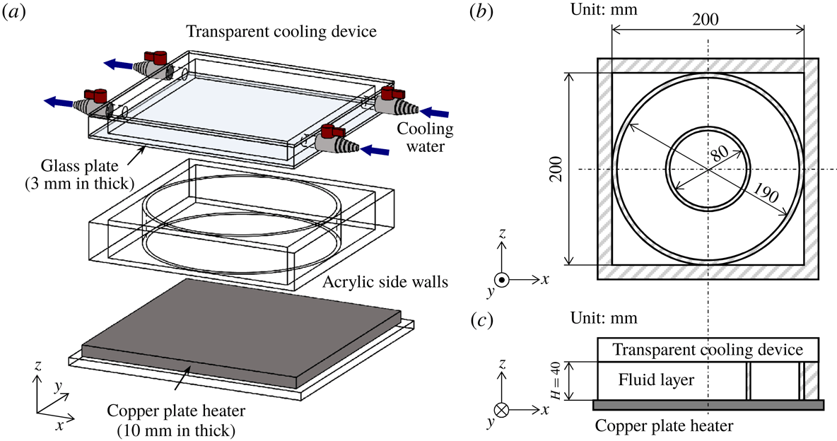
Schematic diagram of the fluid vessel. (a) Overview of the vessel with the acrylic walls, cooling device and copper plate heater. The cylinder inside the square-walled vessel is of diameter $L=190~\text{mm}$ . (b) Horizontal cross-section of the vessel, where two different cylinders ( $L=80$ or $190~\text{mm}$ ) are alternatively placed. (c) Vertical cross-section of the vessel.

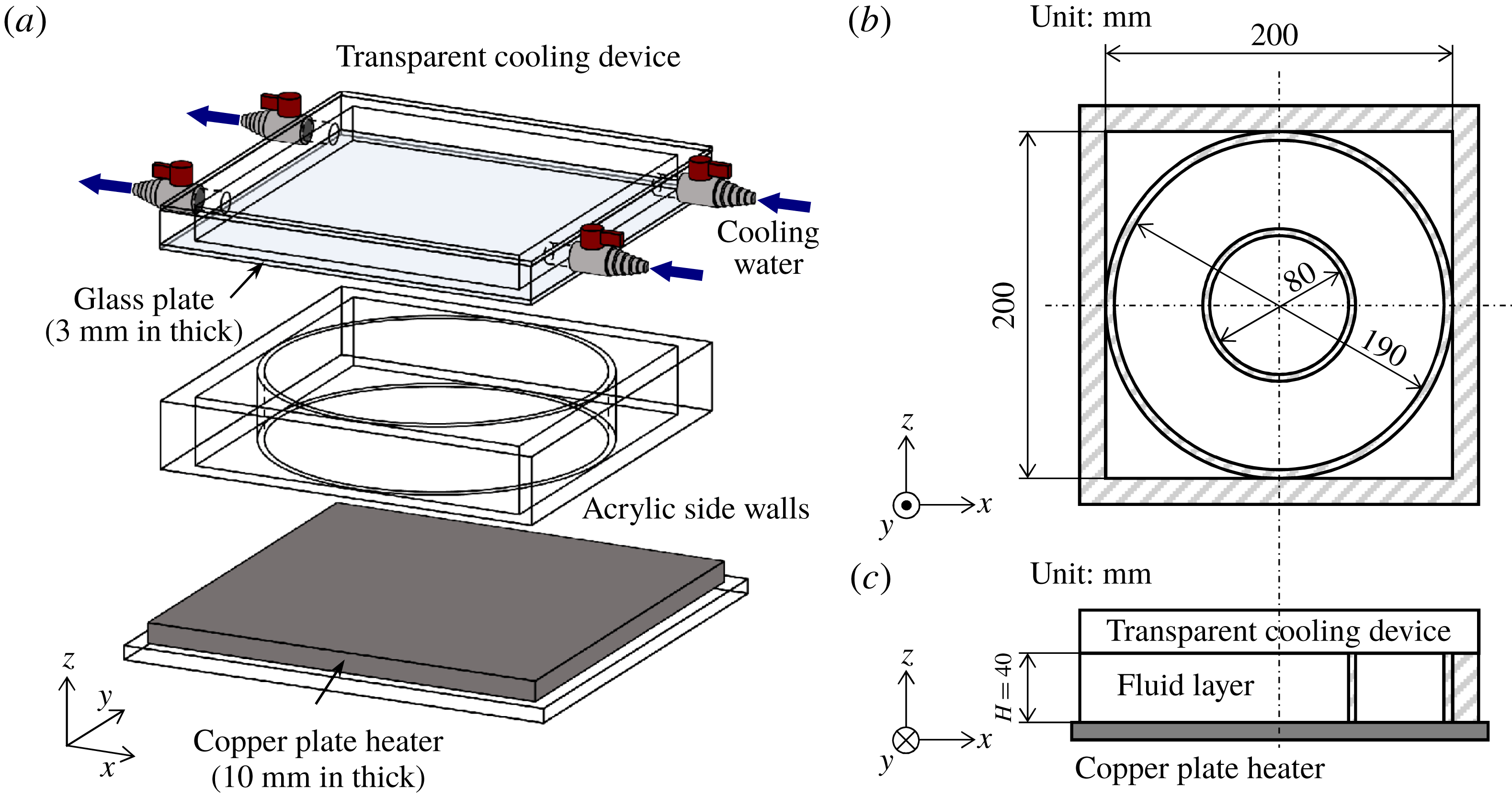
The fluid vessel used in the present study is shown in figure 1. The side walls enclose an acrylic square vessel 200 mm wide and 40 mm high. A cylindrical fluid layer of the same height, $H=40~\text{mm}$ , was formed by placing one of two acrylic cylinders (diameters $L=80$ and 190 mm) in the square vessel allowing easy change in the horizontal geometries. Degassed distilled water ( $Pr\sim 7$ at $20\,^{\circ }\text{C}$ ) was used as the test fluid. A 10 mm thick copper plate heater was set under the bottom of the vessel. Isothermal heating was maintained by controlling the electric current supplied to the heater. The top surface of the vessel was cooled by circulating water from a thermostatic bath via a 3 mm thick glass plate. The corresponding Biot number in the present study is around 0.6 (Noto et al. Reference Noto, Tasaka, Yanagisawa, Park and Murai2018), and preliminary experiments verified the homogeneity of the top cooling condition with this glass plate thickness. The effective temperature difference across the fluid layer was $\unicode[STIX]{x0394}T=11.1\,^{\circ }\text{C}$ measured by thermistors located at the bottom of the copper plate and right beneath the top glass plate. The fluid vessel and all the optical equipment including a camera were mounted on a rotating platform (1 m in diameter with two stages, not shown in figure 1) and rotated together with the vessel and plates. A detailed description of the present experimental apparatus for this rotating RBC is given elsewhere (Noto et al. Reference Noto, Tasaka, Yanagisawa, Park and Murai2018). The angular velocity $\unicode[STIX]{x1D714}$ realized by this set-up is $0.0$ to $5.0~\text{rad}~\text{s}^{-1}$ , corresponding to $Ta=0.0{-}2.8\times 10^{8}$ . 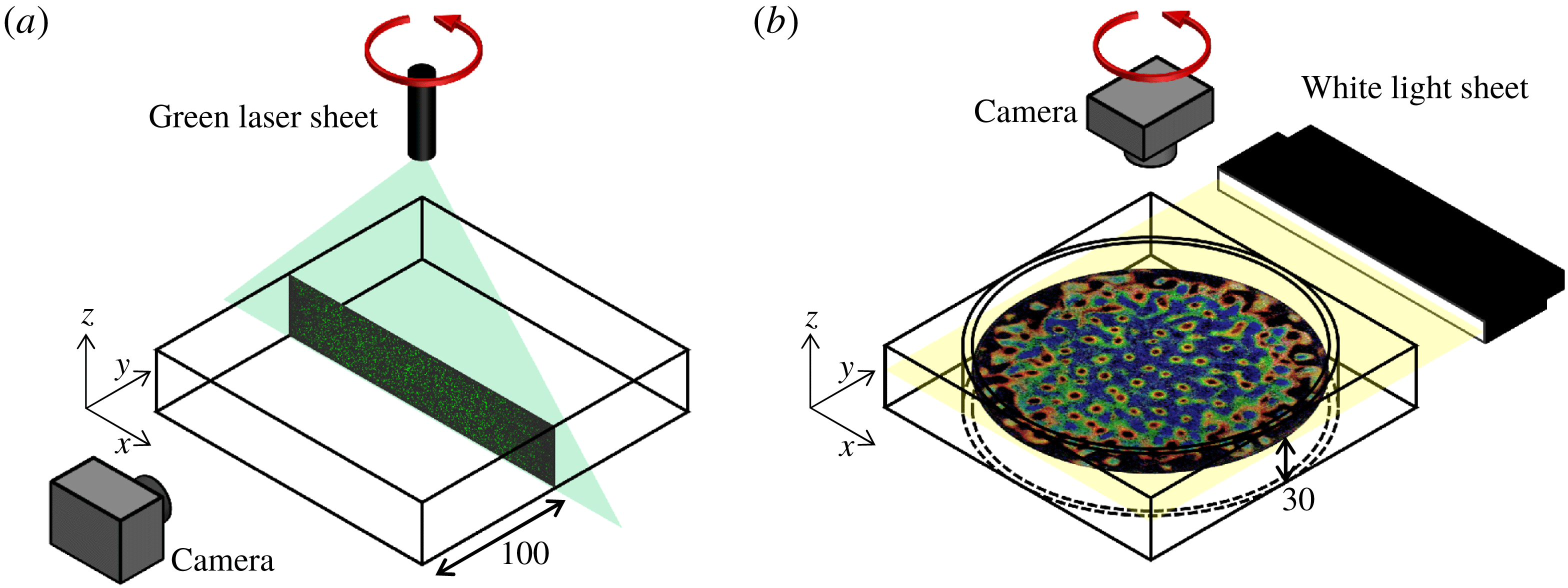Using different configurations of the optical equipment as suggested in figure 2, two different series of experiments were conducted: velocity field measurements of a vertical cross-section (figure 2 a) and temperature field measurements of a horizontal cross-section (figure 2 b). Details of the experiments are described separately in the following sections.

Figure 2.

Optical arrangements for (a) the vertical velocity field measurements by PIV and (b) the horizontal temperature field measurements by TLC particles. Images embedded in each panel are examples obtained by these two different visualization methods. For the experiments, the fluid vessel and optical equipment were placed on a platform and rotated as suggested by the top arrows (red online).

2.2 Velocity field measurements on a vertical cross-section

To perform the PIV measurements of the velocity field on a vertical cross-section, a 2 W green laser sheet ( ${<}$ 5 mm thick) is illuminated from above the cross-section at the middle position ( $y=2.5H$ , 100 mm) of the fluid layer (figure 2 a). No cylinders were placed in the acrylic vessel during the PIV measurements. A small amount of porous resin particles (mean diameter $d_{p}=90~\unicode[STIX]{x03BC}\text{m}$ , mean density $\unicode[STIX]{x1D70C}_{p}=1.02\times 10^{3}~\text{kg}~\text{m}^{-3}$ , HP20SS, Mitsubishi Chemical Co.) were dispersed into the test water and used as flow tracers. The Stokes number $St=\unicode[STIX]{x1D70C}_{p}d^{2}U/(18\unicode[STIX]{x1D70C}\unicode[STIX]{x1D708}H)$ is $O(10^{-4})\ll 1$ , with $\unicode[STIX]{x1D70C}$ the density of the working fluid and $U$ the representative flow velocity (to be detailed below); this will ensure that the tracer particles follow the fluid motions closely. From one side of the vessel, particle images in the $x$ – $z$ plane were recorded using a digital camera (EXF1, Casio) at 5 f.p.s. and a resolution of $0.1~\text{mm}~\text{pixel}^{-1}$ (2000 pixels $\times$ 400 pixels for $200~\text{mm}\times 40~\text{mm}$ ). The images were processed using a standard cross-correlation method to derive instantaneous velocity vector fields from two sequential images.

2.3 Temperature field measurements on a horizontal cross-section

For the temperature field visualization, a white light sheet generated by a halogen lamp illuminated a horizontal cross-section at a set height, $z=0.75H$ (30 mm), of the fluid layer (figure 2 b). A camera, the same as the one used for the PIV experiments, was set at the axis of rotation and recorded colour images of the $x$ – $y$ plane from above the fluid layer. Encapsulated thermochromic liquid crystal (TLC) particles (mean diameter $d_{p}=15~\unicode[STIX]{x03BC}\text{m}$ , mean density $\unicode[STIX]{x1D70C}_{p}=1.02\times 10^{3}~\text{kg}~\text{m}^{-3}$ , approximate dynamic range $20{-}25\,^{\circ }\text{C}$ , Japan Capsular Products Inc.) were suspended in degassed water for the temperature field visualization. 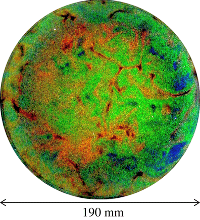Estimated $St$ , $O(10^{-6})$ , ensures sufficiently high traceability of the TLC particles. An example of a temperature field visualized by TLC at no-rotation conditions ( $Ra=1.0\times 10^{7}$ and $Ta=0$ ) obtained in the larger vessel is shown in figure 3. The TLC shows coloration corresponding to the temperature by the scattered incident white light. Typically, red is at the lower end of the colouring temperature range, and the TLC changes scattering colour, from green to light blue to dark blue, as the temperature increases. As shown in figure 3, it is possible to observe red-coloured, cold down-welling flows, and blue-coloured, warm up-welling flows showing the large-scale structures in this condition. The working fluid filled the entire fluid layer including the corner regions outside the cylinders. As a result, the temperature of the ambient fluid is controlled within the set temperature differences playing the role of a water jacket, as well as reducing unwanted reflection of the incident light and provides better quality colour images. The colour images were acquired at three-second intervals ( $\unicode[STIX]{x0394}t=3~\text{s}$ , $1/3$  f.p.s.) with an $f$ -number of 2.7, and a resolution of $0.1~\text{mm}~\text{pixel}^{-1}$ for $\unicode[STIX]{x1D6E4}=2.00$ and $0.1357~\text{mm}~\text{pixel}^{-1}$ for $\unicode[STIX]{x1D6E4}=4.75$ . The TLC is useful for observing the fluid temperature non-invasively. Its calibration from the colour information to temperature is influenced by a number of uncertainties (Wiberg & Lior Reference Wiberg and Lior2004; Abdullah et al. Reference Abdullah, Talib, Jaafar, Salleh and Chonga2010; Rao & Zang Reference Rao and Zang2010). For instance, sensitivity to the incident light yields colorations with a strong dependence on image positions, and the observation direction (the angle measured from the lens) induces similar colour inhomogeneities. To overcome these TLC measurement difficulties, the present study employed localized hue calibration to obtain the temperature fields and applied a robust vortex detection method (Noto et al. Reference Noto, Tasaka, Yanagisawa, Park and Murai2018). In this, the temperature at each pixel was calibrated from locally obtained hue–temperature calibration curves. By combining the vortex detection method with this calibration, it is possible to identify columnar vortices from horizontal temperature fields as undulations at $Pr\sim O(1)$ .

Figure 3.

An example of a horizontal temperature field visualized using the encapsulated TLC at $z=0.75H$ for $Ra=1.0\times 10^{7}$ and $Ta=0$ recorded in the $\unicode[STIX]{x1D6E4}=4.75$ vessel.

3.1 Vertical coherence of vortical structures

Columnar vortical structures, the main focus of the present study, are observed in the transition from a three-dimensional thermal turbulence regime to a CTC regime via a vortical plume regime (Grooms et al. Reference Grooms, Julien, Weiss and Knobloch2010). The emergence of the columnar vortices requires (quasi-)geostrophic conditions that are conventionally assumed at $Ro\ll 1$ . But the parameter boundaries between the regimes must be evaluated in detail in the experiments, and are considerably influenced by side boundaries and centrifugal forces. Consequently, five different conditions, as detailed in table 1, were investigated to evaluate details of the emergence of columnar vortices by PIV measurements. Due to the limitations of the turntable, $Ro$ distributes from 1.20 to 0.12 for the set Rayleigh number, $Ra=1.0\times 10^{7}$ , in the test conditions here. In the following, $N_{vortex}$ is the number of columnar vortices determined in the temperature field image at the horizontal cross-sections of $z=0.75H$ inside a cylinder with $\unicode[STIX]{x1D6E4}=4.75$ (Noto et al. Reference Noto, Tasaka, Yanagisawa, Park and Murai2018). The number of heated vortices present under very similar conditions, $Ro=0.1{-}10$ , in the DNS conducted by Pieri et al. (Reference Pieri, Falasca, Hardenberg and Provenzale2016), is similar to that obtained here (see table 1). Typically, $N_{vortex}$ increases with decreasing $Ro$ , and $N_{vortex}$ strongly depends on the vertical height position. To quantify the vertically distributed characteristics, Rajaei, Kunnen & Clercx (Reference Rajaei, Kunnen and Clercx2017) reported an increase in the vertical coherence with decrease in $Ro$ by PIV experiments. This suggests that the development of columnar vortices may be observed in decreasing $Ro$ conditions in the images of the vertical velocity fields.

Figure 4.

Snapshots of the velocity vector distributions of vertical cross-sections measured in PIV at $y=2.5H$ : (a)  $Ta=1.0\times 10^{6}$ ( $Ro=1.20$ ), (b)  $Ta=6.0\times 10^{6}$ (0.49), (c)  $Ta=1.0\times 10^{7}$ (0.38), (d) $Ta=6.0\times 10^{7}$ (0.15) and (e) $Ta=1.0\times 10^{8}$ (0.12). Only every second vector (the slanted short line (yellow online)) is plotted for clearer visibility.

Table 1.

Parameter settings for the vertical velocity measurements, and measurements of the number of up-welling and down-welling vortices, from Noto et al. (Reference Noto, Tasaka, Yanagisawa, Park and Murai2018).

Examples of the velocity vector distributions measured in the $x$ – $z$ plane at $y=2.5H$ for each $Ta$ setting are shown in figure 4. Here, the magnitude of the measured velocity $\sqrt{u^{2}+w^{2}}$ is rendered in grey scale. Flow structures at low $Ta$ settings, as in figure 4(a–c) are not well organized along the direction of the rotational axis, and only some column-like structures are visible. At high $Ta$ settings (figure 4 d,e), flow structures are recognizable as separate columns. A representative flow velocity is given by Prandtl’s free-fall theory, $U_{f}=\sqrt{g\unicode[STIX]{x1D6FD}\unicode[STIX]{x0394}TH}$ , and here estimated at roughly $U_{f}\sim 30~\text{mm}~\text{s}^{-1}$ . The magnitude of the velocity in rotating RBC is small, at almost only one-tenth of $U_{f}$ because the background rotation is suppressed even when $Ta$ is the smallest. This is also indicated from the fact that the magnitude of the velocity for higher $Ta$ values is lower than that for lower $Ta$ . A typical geostrophic velocity proposed by Sakai (Reference Sakai1997), $U_{0}$ , reflecting a geostrophic balance in the fluid interior, may be obtained from

(3.1) $$\begin{eqnarray}U_{0}=\frac{\unicode[STIX]{x1D705}}{2l}\left(\frac{\unicode[STIX]{x0394}T_{c}}{\unicode[STIX]{x0394}T}\right)RaTa^{-1/2},\end{eqnarray}$$

where $\unicode[STIX]{x0394}T_{c}$ is the temperature difference between up-welling and down-welling vortices when the vertical temperature of the columns is constant, and the columns are separated by a distance $l$ . Under the present conditions, $U_{0}$ is of order $O(1~\text{mm}~\text{s}^{-1})$ , which would agree well with the present results.

Figure 5.

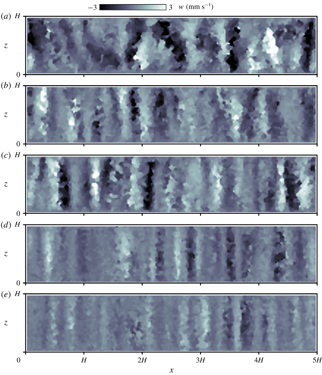
Vertical velocity distributions $w(x,z)$ in vertical cross-sections at the same moment as that of figure 4 measured by PIV at $y=2.5H$ : (a)  $Ta=1.0\times 10^{6}$ ( $Ro=1.20$ ), (b)  $Ta=6.0\times 10^{6}$ (0.49), (c)  $Ta=1.0\times 10^{7}$ (0.38), (d) $Ta=6.0\times 10^{7}$ (0.15) and (e)  $Ta=1.0\times 10^{8}$ (0.12).

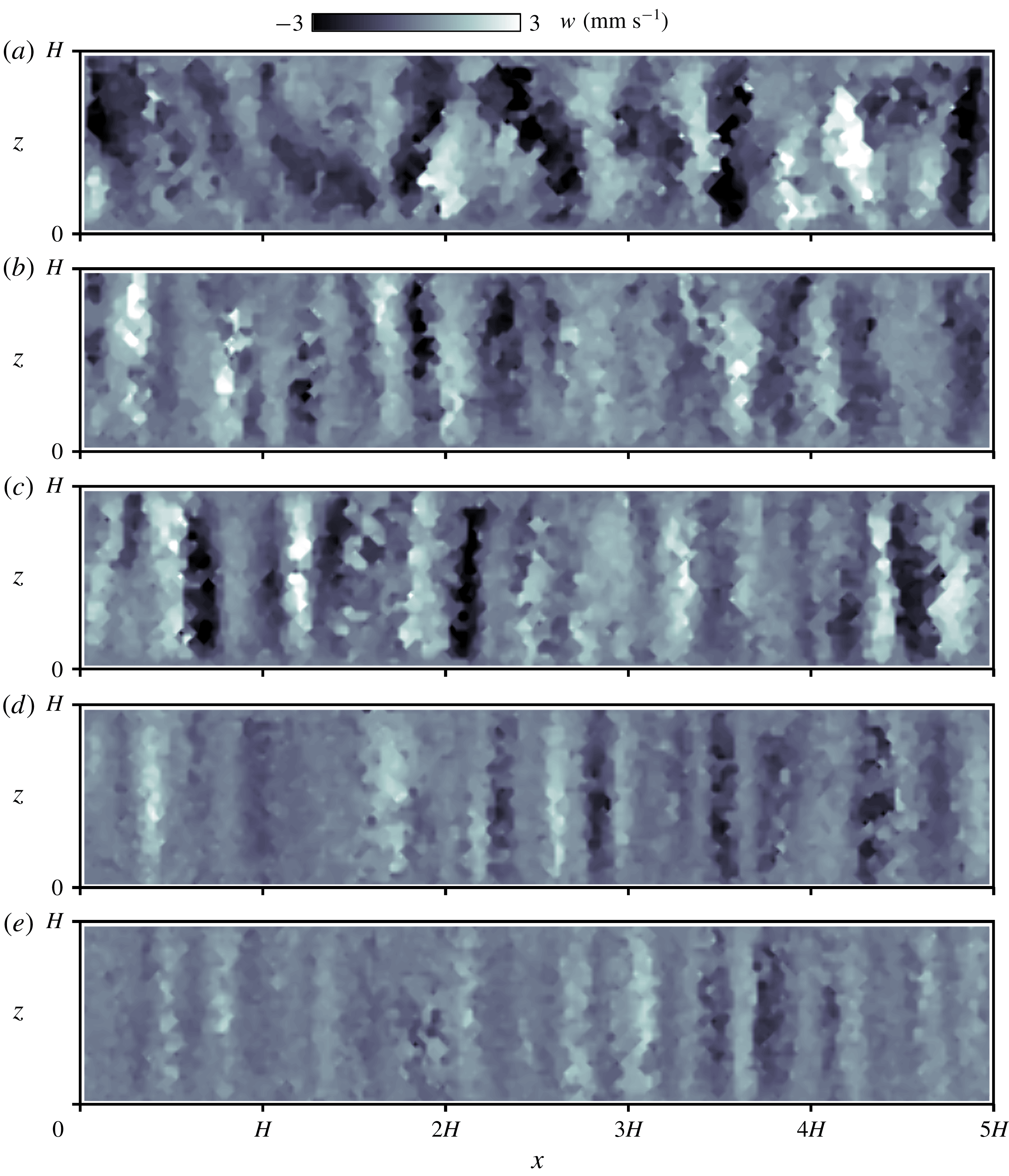
To highlight the vertical coherence of the flow structures, the corresponding distributions of the vertical velocity $w$ for the images shown in figure 4 were also calculated and are shown in figure 5. While somewhat disorganized, structures are visible in figure 5(a). These are vertical coherent structures from bottom to top (bright), and from top to bottom (dark), aligned alternately in horizontal directions in the other cases satisfying $Ro<1$ . These indicate up-welling and down-welling flows that arise from Ekman pumping. The structures appear increasingly regularized in the vertical direction with increasing $Ta$ ; the horizontal distance (left–right in the figure) between the structures also becomes shorter. In a previous report (Noto et al. Reference Noto, Tasaka, Yanagisawa, Park and Murai2018), the distance between neighbouring structures at each setting was found to agree well with the theory established by Sakai (Reference Sakai1997). Fluctuations of the velocity in the vertical direction diminish with $Ta$ with the structure appearing as a quasi-2-D regular column in figure 5(d,e), specifically, at $Ro=0.15$ and 0.12. Further quantitative criteria to distinguish prominent columnar vortices are discussed in the next section.

3.2 Local duration characteristics of columnar vortices

In the previous section, spatial, instantaneous quasi-2-D columnar structures were analysed. To investigate the translational motion of columnar vortices, the duration of vertical coherence also needs to be investigated in regard to the time variation in the appearance. This is required to verify that the vortices detected on the horizontal plane in sequential images exhibit translational motion and not a continuous skewed deformation. This also has importance in determining a suitable time resolution for vortex tracking. One advantage of TLC visualization is that detection of the vortices may be achieved from a single instantaneous image with a wider flexible range of time resolutions than in PIV requiring two consecutive images taken within a short time interval (Noto et al. Reference Noto, Tasaka, Yanagisawa, Park and Murai2018).

Considering the results obtained with PIV, in particular those in figure 5(d,e), the sign of the vertical velocity $w$ along a single columnar vortex is the same from top to the bottom and in the image. This is because all the columnar vortices can be classified as up-welling ( $w>0$ ) or down-welling ( $w<0$ ) vortices. As Rajaei et al. (Reference Rajaei, Kunnen and Clercx2017) showed, vertical coherence of columnar vortices can be obtained by making auto-correlations of vorticity along the rotational axis, when all of the velocity information (three-dimension and three-component) is available. In the present study, the available information is the velocity field only in the $x$ – $z$ plane, and it is necessary to show vertical coherence of the columnar vortices in this condition. Hence, the averaged vertical velocity $\overline{w(x,t)}=(1/H)\int _{0}^{H}w(x,z,t)\,\text{d}z$ is a useful indicator to identify column formation. To establish the time variation of the vertical coherence, the evolution of $\overline{w(x,t)}$ with elapsed time is plotted (figure 6). In figure 6 the values have been normalized using the maximum of the absolute value. The two-headed arrows in each panel are equivalent to the theoretically predicted diameters of the vortices, $L_{vortex}$ , derived by Sakai (Reference Sakai1997) and as will be defined below. In figure 6(a,b), the bright and dark stripes do not maintain the same width throughout the observation period. A zero value of $\overline{w(x,t)}$ indicates the absence of columns. With a larger $Ta$ setting, figure 6(c–e) shows a straight striped pattern. The columns appear at very similar positions, at least within the observation period for the larger $Ta$ settings here. In addition, there are variations in the width of the stripes. Assuming that the widths of the columnar vortices are constant in the horizontal direction, these variations arise from plane displacements, specifically, column displacements in the $y$ direction; skewed stripes indicate displacements in the $x$ direction.

Figure 6.

Time series of averaged vertical velocities at horizontal positions $2H<x<3H$ : (a)  $Ta=1.0\times 10^{6}$ $(Ro=1.20)$ , (b)  $Ta=6.0\times 10^{6}$ (0.49), (c)  $Ta=1.0\times 10^{7}$ (0.38), (d)  $Ta=6.0\times 10^{7}$ (0.15) and (e)  $Ta=1.0\times 10^{8}$ (0.12). Two-headed arrows indicate the theoretically predicted diameter of the columnar vortices $L_{vortex}$ derived by Sakai (Reference Sakai1997).

Assuming that the horizontal motion of the vortices is isotropic, the advection speed of the columnar vortices may be estimated simply from the slopes of the stripes:

(3.2) $$\begin{eqnarray}v_{adv}=\sqrt{\left(\frac{\text{d}x}{\text{d}t}\right)^{2}+\left(\frac{\text{d}y}{\text{d}t}\right)^{2}}\sim \sqrt{2\left(\frac{\text{d}x}{\text{d}t}\right)^{2}},\end{eqnarray}$$

with $v_{adv}$ indicating the horizontal advection speed of the columnar vortices. From these estimates the maximum value of $v_{adv}$ is $O(0.1{-}1~\text{mm}~\text{s}^{-1})$ . With this, the time resolution for the vortex tracking of the horizontal cross-sections becomes $O(1~\text{s})$ under the present optical conditions.

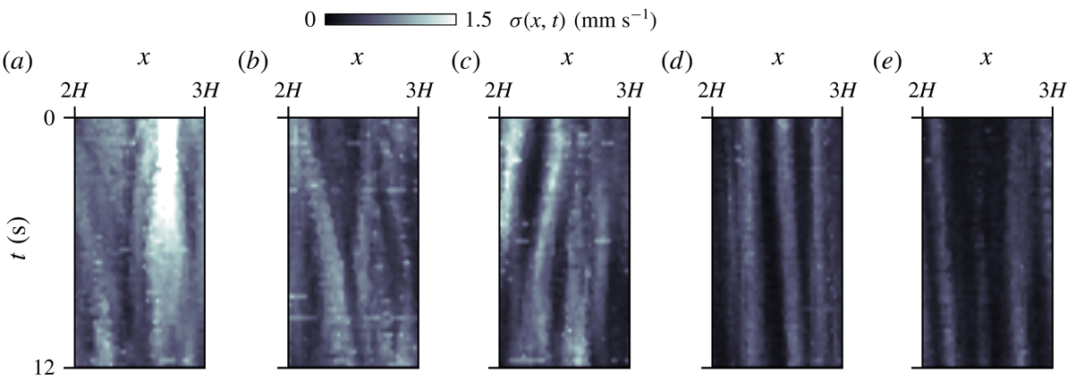
In addition to the vertical average, the standard deviation of $w$ , obtained from $\unicode[STIX]{x1D70E}(x,t)^{2}=(1/H)\int _{0}^{H}[w(x,z,t)-\overline{w(x,t)}]^{2}\,\text{d}z$ , gives another estimate of the vertical coherence. The standard deviations, $\unicode[STIX]{x1D70E}(x,t)$ , for each of the periods in the images of figure 6 are presented in figure 7. At lower $Ta$ settings, the high magnitude of $\unicode[STIX]{x1D70E}(x,t)$ indicates that $w$ varies along the $z$ axis. Accordingly, if the vertically straight (coherent) columns maintain their structures during this observation time, the magnitude of $\unicode[STIX]{x1D70E}(x,t)$ does not change at the same horizontal positions. For this reason, it is difficult to identify columns possessing system height structures for the lowest two $Ta$ settings. A spatiotemporal integration (average) of $\unicode[STIX]{x1D70E}(x,t)$ , $\overline{\unicode[STIX]{x1D70E}}=(1/LT)\int _{0}^{L}\int _{0}^{T}\unicode[STIX]{x1D70E}(x,t)\,\text{d}x\,\text{d}t$ , suggests how stable the columnar vortices are, allowing the local characteristics of the duration of the columnar vortices to be quantified. This is because a smaller value of the spatiotemporal integration of the vertical variance signifies vertical coherence of the columnar vortices. The variations in $\overline{\unicode[STIX]{x1D70E}}$ with $Ta$ are shown in figure 8; here, the dashed line shows the fitted curve calculated by the least-squares method. In the present study, the curve obtained is $\overline{\unicode[STIX]{x1D70E}}/U_{f}=0.026Ro^{0.47}$ . As $Ro$ approaches zero, the flow structures maintain vertical coherence here. For low $Ro$ values there is a cellular regime (Cheng et al. Reference Cheng, Stellmach, Ribeiro, Grannan, King and Aurnou2015), where no visible vortex motion appears. This suggests that the results obtained in this analysis may be considered as reasonably accurate. In figure 8, the ratio of $\overline{\unicode[STIX]{x1D70E}}$ to $U_{f}$ is ${\sim}0.01$ for the two highest $Ta$ settings, with only 1 % of deviation from the free-fall velocity $U_{f}$ .

Figure 7.

Time series of the standard deviations for the vertical velocity component at horizontal positions $2H<x<3H$ : (a)  $Ta=1.0\times 10^{6}$ ( $Ro=1.20$ ), (b)  $Ta=6.0\times 10^{6}$ (0.49), (c)  $Ta=1.0\times 10^{7}$ (0.38), (d)  $Ta=6.0\times 10^{7}$ (0.15) and (e)  $Ta=1.0\times 10^{8}$ (0.12).

Figure 8.

Variation of local duration characteristics $\overline{\unicode[STIX]{x1D70E}}$ plotted with error bars giving the standard deviation. Here, $\overline{\unicode[STIX]{x1D70E}}$ is normalized by the free-fall velocity $U_{f}$ . The dashed line is a least-squares fit of $\overline{\unicode[STIX]{x1D70E}}/U_{f}=0.026Ro^{0.47}$ .

To track the translational motion of the columnar vortices further, the points discussed in this section may be summarized as follows. The vortical structures exhibit two-dimensionality in the velocity distributions on the vertical cross-sections. Skewed structures along the $z$ axis represent a three-dimensional turbulence-like state for the lowest $Ta$ settings. With the time variation of $w$ , a horizontal advection speed of the columns, $v_{adv}$ , could be estimated. The estimated value of $O(0.1{-}1~\text{mm}~\text{s}^{-1})$ suggests an appropriate time resolution for vortex tracking of every few seconds ensuring that the detailed time resolution avoids erroneous tracking. In addition, the number of up-welling and down-welling vortices is also a good indicator of the flow state. An almost equal number of these in the same horizontal cross-section indicates (fully) developed CTC (see table 1). In summary, columnar vortices with $Ta\geqslant 1.0\times 10^{7}$ ( $Ro\leqslant 0.15$ ) ensure a horizontal translational motion of the columnar vortices in the present study.

4.1 Vortex detection from horizontal temperature field

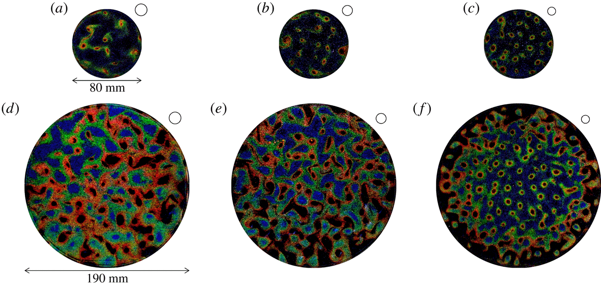
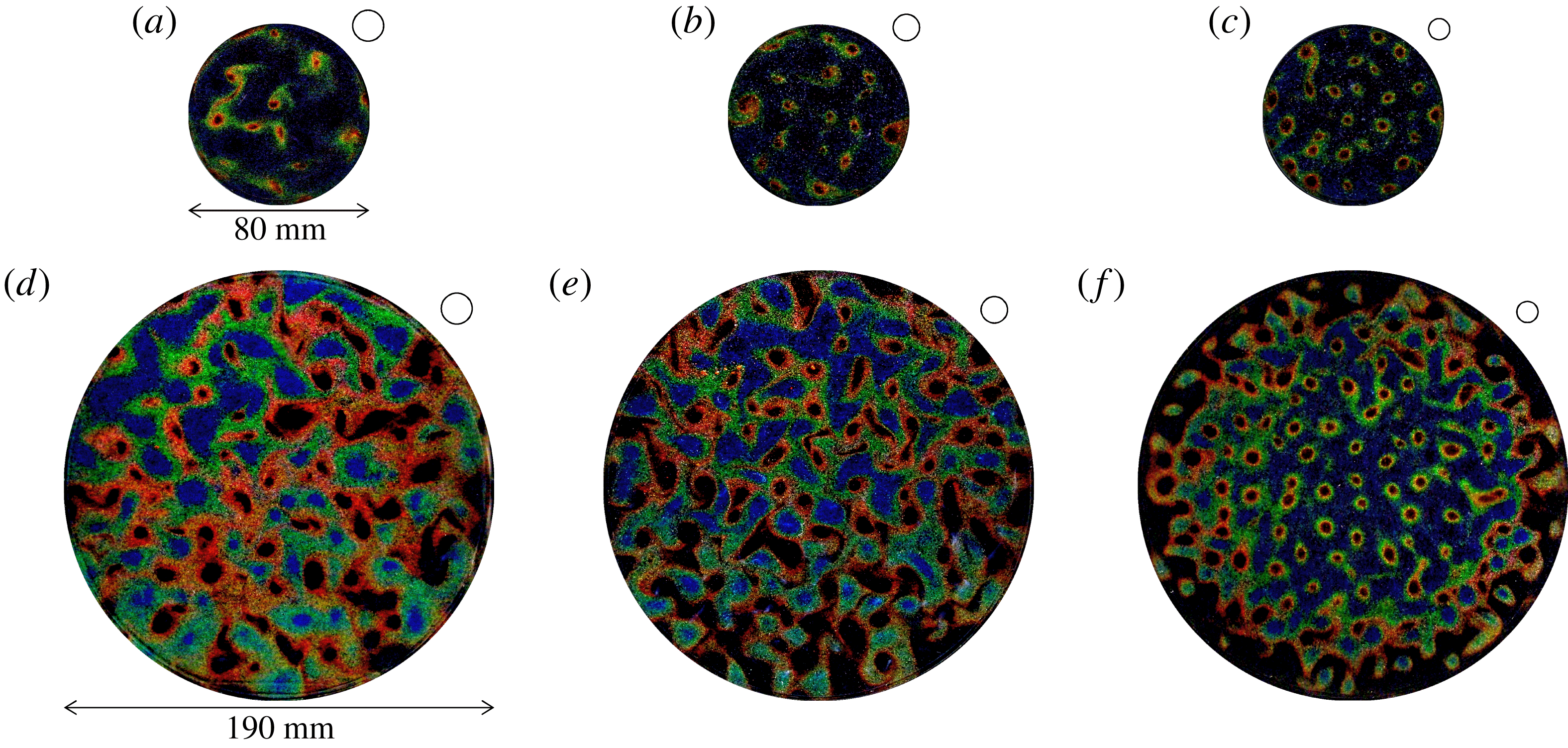
Using encapsulated TLC particles, we were able to develop images of the temperature field (figure 9) to visualize the columnar vortices. Heated up-welling and cooled down-welling vortical structures are simply recognized as blue and red circular colour variations. For both $\unicode[STIX]{x1D6E4}$ instances, finer and more organized structures with increasing $Ta$ were found to be common changes. The horizontal scale of these vortical structures, denoted $L_{vortex}$ , was predicted in previous work. At the onset of convection, Chandrasekhar (Reference Chandrasekhar1961) using linear stability theory derived $L_{vortex}=cHTa^{-1/6}$ with the prefactor $c=4.8$ . Differently, Cheng et al. (Reference Cheng, Aurnou, Julien and Kunnen2018) found $c=2.4$ taking Ekman pumping into account with $Ta<10^{14}$ . In water experiments without a rigid top boundary, Boubnov & Golitsyn (Reference Boubnov and Golitsyn1986) found an empirical scaling $L_{vortex}=Ra^{1/9}Ta^{-1/4}$ using the present notation. Sakai (Reference Sakai1997) derived a theoretical scaling law by considering a physical model with two rigid boundaries and verified its adequacy experimentally. From his estimate, the horizontal scale of columnar vortices $L_{vortex}$ is

(4.1) $$\begin{eqnarray}L_{vortex}=4.6H\frac{\unicode[STIX]{x1D6FF}_{t}^{2}}{2\unicode[STIX]{x1D6FF}_{t}^{2}+2\unicode[STIX]{x1D6FF}_{t}\unicode[STIX]{x1D6FF}_{E}+\unicode[STIX]{x1D6FF}_{E}^{2}}Ra^{1/3}Ta^{-3/8},\end{eqnarray}$$

where $\unicode[STIX]{x1D6FF}_{t}$ and $\unicode[STIX]{x1D6FF}_{E}$ denote the thickness of the thermal and Ekman boundary layers, respectively. Under set $Ra$ conditions, $L_{vortex}$ depends on only $Ta$ . Our previous work (Noto et al. Reference Noto, Tasaka, Yanagisawa, Park and Murai2018) established a vortex determination method from instantaneous temperature fields using this estimate. On actual colour images, temperature values are reliably related to hue values, which directly shows the colour itself as a degree such as $0^{\circ }$ for red, $120^{\circ }$ for green and $240^{\circ }$ for blue. This is useful for calibrating coloration to temperature, even though the uncertainty is not negligible. In the horizontal temperature fields obtained through this colour–temperature calibration, columnar vortices can be regarded as temperature undulations similar to a point spread function – a 2-D Gaussian distribution. This is because the temperature inside the down-welling (or up-welling) vortex gradually decreases (increases) towards the centre, and these facts result in the concave (convex) temperature distribution inside the vortex (e.g. figure 6 in Noto et al. Reference Noto, Tasaka, Yanagisawa, Park and Murai2018). Such concave or convex undulations can be extracted using pattern recognition techniques. In the present study, the same method was employed to detect columnar vortices of horizontal cross-sections.

Figure 9.

Examples of horizontal temperature fields visualized using encapsulated TLCs at $z=0.75H$ for (a)  $Ta=1.0\times 10^{7}$ , (b)  $Ta=3.0\times 10^{7}$ and (c)  $Ta=1.0\times 10^{8}$ with $\unicode[STIX]{x1D6E4}=2.00$ , and (d) $Ta=1.0\times 10^{7}$ , (e)  $Ta=3.0\times 10^{7}$ and (f)  $Ta=1.0\times 10^{8}$ with $\unicode[STIX]{x1D6E4}=4.75$ . Open circles appearing on the upper right of each image indicate the horizontal scale of the columnar vortices predicted by Sakai (Reference Sakai1997).

4.2 Statistical characteristics of advection velocity of columnar vortices

As $Ro$ approaches zero, the number of up-welling and down-welling vortices approaches a balance (Vorobieff & Ecke Reference Vorobieff and Ecke2002). Assuming a balanced population and columnar vortices in vertical coherence, then only one, for example the down-welling, vortex motion needs to be investigated. (The centrifugal force discussed below, however, may affect statistical motions of up- and down-welling vortices and push vortices in the opposite directions.) Image acquisition was conducted for a one-hour period after reaching a fully developed flow state (more than 30 min from initiating the rotation). Around 1200 consecutive images and temperature fields were obtained. The nearest-neighbour method was employed to track the labelled vortices on the visualized temperature fields, in which two vortices having the shortest Euclidean distance between two consecutive images are linked. The vortex advection speed $v_{adv}$ can then be obtained using

(4.2) $$\begin{eqnarray}v_{adv}=\frac{|\boldsymbol{r}(t+\unicode[STIX]{x0394}t)-\boldsymbol{r}(t)|}{\unicode[STIX]{x0394}t},\end{eqnarray}$$

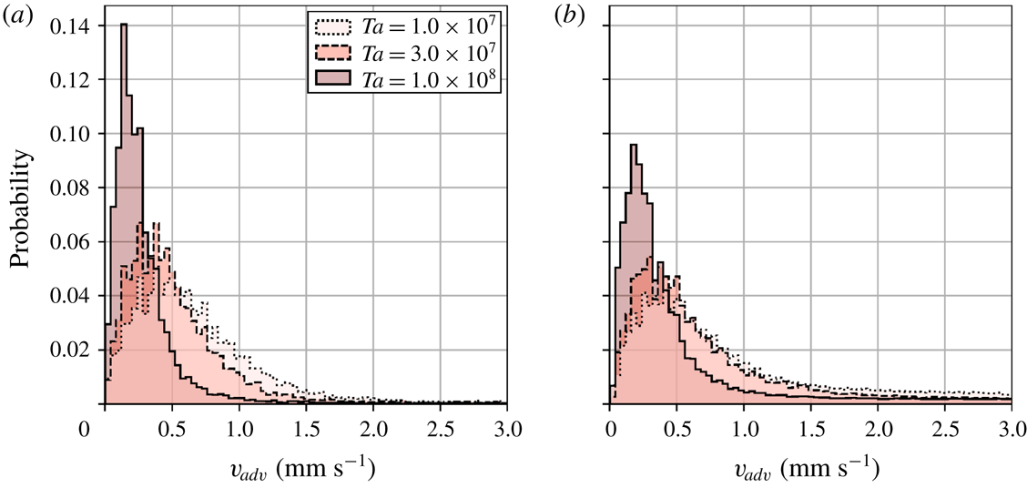
where $\boldsymbol{r}(t)$ denotes the vortex position vector obtained by the vortex detection method (Noto et al. Reference Noto, Tasaka, Yanagisawa, Park and Murai2018). The probability distributions of $v_{adv}$ for all our settings of $Ta$ and $\unicode[STIX]{x1D6E4}$ were plotted and analysed (figure 10).

Figure 10.

Probability distributions of horizontal advection speeds of columnar vortices $v_{adv}$ for three different values of $Ta$ ; (a)  $\unicode[STIX]{x1D6E4}=2.00$ and (b)  $\unicode[STIX]{x1D6E4}=4.75$ .

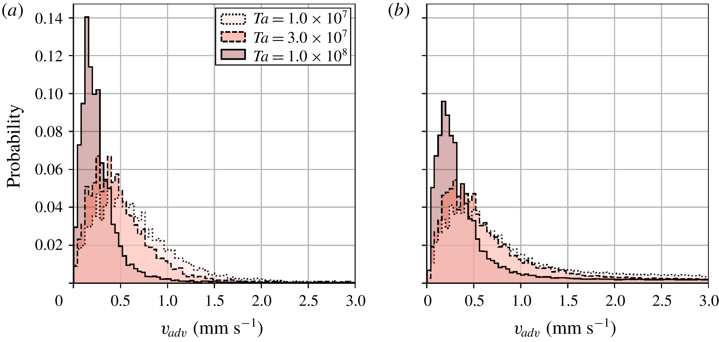
From all the conditions examined, the horizontal translational motion of columnar vortices is extremely slow compared with that of each of the flow fields (figure 10). Specifically, $v_{adv}$ is $O(10^{-1}~\text{mm}~\text{s}^{-1})$ whereas a typical geostrophic velocity $U_{0}$ is $O(10^{0}~\text{mm}~\text{s}^{-1})$ . Moreover, $v_{adv}$ decreases as $Ta$ increases. This result is consistent with a transition from the CTC regime to the cellular regime as $Ta$ increases. Basically, the distributions are quite similar for vessels of different aspect ratios, except for the highest $Ta$ setting with the larger aspect ratio, where the corresponding $Fr$ value is close to 0.1. Considering only the difference in the cylinder radii, an obvious difference under this condition may therefore come from the effect of the centrifugal force, even though all the present conditions are satisfying the conventional criterion to disregard any influence of centrifugal forces, $Fr<0.1$ . 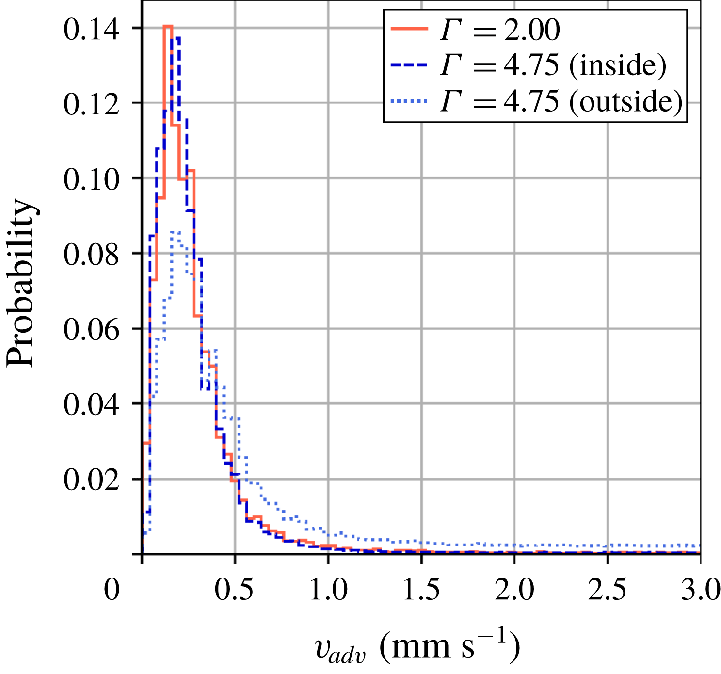To confirm this possibility, the probability distribution for columnar vortices present inside the region $r\leqslant 40~\text{mm}$ for the $\unicode[STIX]{x1D6E4}=4.75$ vessel (corresponding to $\unicode[STIX]{x1D6E4}\leqslant 2.00$ ) is replotted (figure 11), here labelled $\unicode[STIX]{x1D6E4}=4.75$ (inside) to separate the effect of centrifugal force. The distribution of $\unicode[STIX]{x1D6E4}=4.75$ (inside) agrees well with that of $\unicode[STIX]{x1D6E4}=2.00$ . 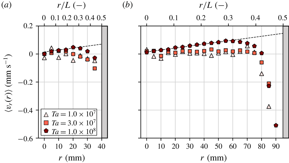The probability distribution outside the region $r>40~\text{mm}$ , labelled $\unicode[STIX]{x1D6E4}=4.75$ (outside), shifts slightly towards the higher-speed region compared with that for the inside region. In addition to this separately plotted histogram, the averaged radial components of advection speeds $v_{adv}$ at each radial position, $\langle v_{r}(r)\rangle$ , are examined to understand details of the effect of the centrifugal force. The averaged speed $\langle v_{r}(r)\rangle$ is defined as

(4.3) $$\begin{eqnarray}\langle v_{r}(r)\rangle =\frac{1}{N}\mathop{\sum }_{i=1}^{N}(v_{xi}\cos \unicode[STIX]{x1D703}_{i}+v_{yi}\sin \unicode[STIX]{x1D703}_{i}),\end{eqnarray}$$

plotted in figure 12, where $v_{x}$ and $v_{y}$ are the $x$ and $y$ components of the advection velocity of columnar vortices located at $(r,\unicode[STIX]{x1D703})$ in polar coordinates. A gradual increase is observed in the larger vessel at $Ta=1.0\times 10^{8}$ (figure 12 b) in concert with increases in $r$ . Especially in the range of $0\leqslant r<60~\text{mm}$ , $\langle v_{r}(r)\rangle$ is linearly proportional to the radial distance $r$ with a slope of $0.0014$ according to a least-squares fit in this range. It is noteworthy that the plot with the smaller vessel at $Ta=1.0\times 10^{8}$ fits the same line (slope) as shown in figure 12(a). Other conditions are everywhere in near $v_{r}=0$ and it is difficult to identify any significant dependence on the radial position, except for the vicinity of the wall. Sudden drops of the velocity in the region corresponding to radially inward movement start at $r\sim 0.35L$ – $0.4L$ ( $r\sim 28{-}32~\text{mm}$ for $\unicode[STIX]{x1D6E4}=2.00$ and $r\sim 67{-}76~\text{mm}$ for $\unicode[STIX]{x1D6E4}=4.75$ ) for all $Ta$ conditions. These originate in repulsion by wall collisions. The standard deviations of each plot are roughly in the range of $0.2{-}0.6~\text{mm}~\text{s}^{-1}$ , and increase as $Ta$ decreases. These results suggest the conclusion that the centrifugal force working on each columnar vortex as a body force may be seen as the main reason for the differences in the distribution for this $Ta$ setting, although heuristically the effects of the centrifugal force have been assumed negligibly small when $Fr<0.1$ (Cheng et al. Reference Cheng, Aurnou, Julien and Kunnen2018). The influence of centrifugal forces on the vortex motion will be discussed in the next section.

Figure 11.

Probability distribution at $Ta=1.0\times 10^{8}$ with $\unicode[STIX]{x1D6E4}=2.00$ (solid line) and separated plots of $\unicode[STIX]{x1D6E4}=4.75$ from different regions: (inside) $r\leqslant 40~\text{mm}$ (dashed line) and (outside) $r>40~\text{mm}$ (dotted line).

Figure 12.

Radial position dependence of ensemble-averaged radial advection velocity $\langle v_{r}\rangle$ : (a)  $\unicode[STIX]{x1D6E4}=2.00$ and (b)  $\unicode[STIX]{x1D6E4}=4.75$ . Each plot is an average of 5 mm domains. Dashed line is $\langle v_{r}(r)\rangle =0.0014r+0.0143$ obtained by a least-squares fit.

An approximate evaluation of the probability density distributions suggests that their shape is similar to a Maxwell distribution assuming a probability density function with more frequent low energies (speed) and fewer high energies. If this is reasonably satisfied, translational motion of the columnar vortices can be regarded as diffusive motion, similar to Brownian motion. An attempt to fit the histograms (figure 10) by the Maxwell distribution,

(4.4) $$\begin{eqnarray}P_{M}(v)=Av\exp (-v^{2}/B),\end{eqnarray}$$

was performed using the least-squares approximation (figure 13). The classical assumptions underpinning this distribution for the particle speed are that the particles initially move randomly, and form an idealized gas that is spatially homogeneous (independent of their position) and which is isotropic. Quite large deviations from the fitted curves are seen, especially in the high-speed region. Table 3 lists the fitting constants, $A$ and $B$ , and three speeds of vortex advection, here denoted $v_{mp}$ , $v_{ave}$ and $v_{rms}$ . They signify respectively the most probable speed satisfying $\text{d}P(v_{mp})/\text{d}v=0$ , the average speed and the root-mean-squared speed. For brevity, $v_{adv}$ is expressed as $v$ in the above equation. These velocities may also be calculated from the fitted curves; $v_{mp}$ is given as $v_{mp}=\sqrt{B}$ . It is clear that the speeds depend on $Ta$ conditions, although the quality of the fit by the Maxwell distribution with classical assumptions is not perfect. The reasons for the discrepancy will be assessed in the next section and form the main purpose of this paper.

Figure 13.

Probability density functions fitted by the Maxwell distribution; the original probability density function data are from figure 10 for the three different $Ta$ settings with (a)  $\unicode[STIX]{x1D6E4}=2.00$ and (b)  $\unicode[STIX]{x1D6E4}=4.75$ vessels.

Table 3.

Advection speeds of columnar vortices.

4.3 Tracking of the multi-time-scale behaviour of columnar vortices

With only the instantaneous observations of the motion of columnar vortices, the deviations from the probability distributions in the Maxwell distributions are difficult to explain. To provide a more detailed description of the vortex motion, a quantification of the differences between actual and idealized particles was performed. The differences arise because of the presence of strong mutual interactions and external (centrifugal) forces. Rather than the analysis of discrete sequences of observations, continuous observations of the vortex motion would serve this purpose. In preparation for this, the lifetime $t_{life}$ of columnar vortices needs to be determined to establish the time scales in which the mutual interactions are appreciable. For the time intervals where an individual vortex is tracked, $t_{life}$ may also be established (see Noto et al. 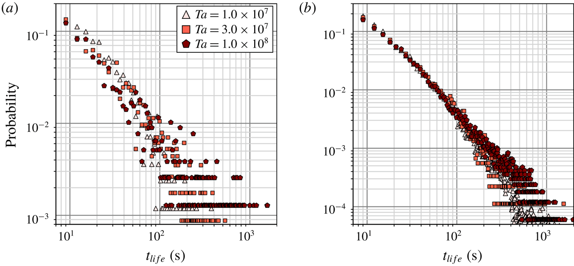Reference Noto, Tasaka, Yanagisawa, Park and Murai2018); in the determination a vortex is deemed to be created at its first detection in a temperature field, and its disappearance through merging defines the end of its presence in the series of observations. The probability distribution for $t_{life}$ during one hour of observations is then extracted based on this definition (figure 14). Columnar vortices have lifetimes distributed mainly from 10 to 100 s in both vessels here. For $\unicode[STIX]{x1D6E4}=2.00$ in figure 14(a), there is a clear $Ta$ dependence on $t_{life}$ ; vortices have shorter lifetimes at lower $Ta$ values. With $\unicode[STIX]{x1D6E4}=4.75$ in figure 14(b), however, the $Ta$ dependence is less clear. The reason may be because centrifugal forces are affecting the vortex motion. The sampled number of vortices for the smaller vessel is smaller than that for the larger vessel; however, the two plots show similar advection changes, suggesting that the advection may be determined by the advection speed in the finite fluid layer and interactions with the surrounding vortices. The differences along the vertical axis are suggested to stem from the sampled number of vortices and to arise from the differences in the aspect ratio. In the present conditions, frequent merging events have been reported in several previous experimental works (Boubnov & Golitsyn Reference Boubnov and Golitsyn1986; Zhong et al. Reference Zhong, Ecke and Steinberg1993; Noto et al. Reference Noto, Tasaka, Yanagisawa, Park and Murai2018) and numerical works (Julien et al. Reference Julien, Legg, McWilliams and Werne1996; Pieri et al. Reference Pieri, Falasca, Hardenberg and Provenzale2016) as arising from the absence of sheath structures with vorticities of opposite signs. The historicity, position dependence and strong mutual interaction within the surroundings may be the cause of the discrepancies appearing in the quality of the fit described in the previous section. Considering the variations in vortex motion which depend on the observation time scale, vortex lifetimes are very important. This is because the forces affecting the vortices and the heat carried by the vortices are both dependent on the vortex lifetime. From the observed phenomena and the various lifetimes of the vortices, three time scales may be postulated: a short time scale $O(10^{0}{-}10^{1}~\text{s})$ where no vortex–vortex interactions occur, an intermediate time scale $O(10^{1}{-}10^{2}~\text{s})$ where strong mutual interactions occur and a long time scale $O(10^{2}{-}10^{3}~\text{s})$ where the effects of external forces (centrifugal forces) emerge.

Figure 14.

Probability distributions of lifetimes $t_{life}$ of columnar vortices for (a)  $\unicode[STIX]{x1D6E4}=2.00$ and (b)  $\unicode[STIX]{x1D6E4}=4.75$ .

To further substantiate this, an analysis of the instantaneous vortex behaviour, as well as vortex tracking by time scales $O({>}10^{1}~\text{s})$ in which the various forces act on the vortex motion, including their advection history, must be conducted. Noto et al. (Reference Noto, Tasaka, Yanagisawa, Park and Murai2018) reported quasi-regular vortex arrangements obtained in 90 s periods for larger $Ta$ settings, and suggested the possibility of describing vortex motion as an $n$ -body problem. Path lines of vortex advection at these time scales (during $30\unicode[STIX]{x0394}t$ ; 90 s) were plotted (figure 15). In figure 15, path lines of down-welling columns present in one period (90 s) were cropped and redrawn using colour coding to represent the elapsed time. Depending on the number of vortices, the number of path lines increases with $Ta$ , and from figure 10 the displacement in one time step (3 s) becomes larger as $Ta$ decreases. The path lines in figure 15(a,b,d,e) appear to be random walks, with no directivity. With high $Ta$ values in both vessels here (figure 15 c,f), the path lines show weak regularity with the directions of movement restricted by surrounding path lines. As two vortices of opposing vorticity cannot merge (Sprague et al. Reference Sprague, Julien, Knobloch and Werne2006), this suggests why so few path lines are observed. With the presence of adjacent up-welling vortices, the motion of down-welling vortices tracked here is directional. Further, the repulsion from up-welling vortices cannot be ignored in this situation, as Julien et al. (Reference Julien, Legg, McWilliams and Werne1996) observed when strong vortex–vortex interactions were present. The path lines for high $Ta$ values may, therefore, be assumed not to represent random motion as shown by Brownian particles.

Figure 15.

Path lines for advections of the columnar vortices for 90 s: (a)  $Ta=1.0\times 10^{7}$ , (b)  $Ta=3.0\times 10^{7}$ and (c)  $Ta=1.0\times 10^{8}$ with $\unicode[STIX]{x1D6E4}=2.00$ , and (d)  $Ta=1.0\times 10^{7}$ , (e)  $Ta=3.0\times 10^{7}$ and (f)  $Ta=1.0\times 10^{8}$ with $\unicode[STIX]{x1D6E4}=4.75$ , where the evolution of the path lines is displayed using colour coding. Backgrounds are grey for better visibility.

In addition to the analysis at the intermediate time scales $O(10^{1}{-}10^{2}~\text{s})$ , vortex tracking over much longer time scales $O(10^{2}{-}10^{3}~\text{s})$ may be performed simply by using the vortex detection method from the images (Noto et al. Reference Noto, Tasaka, Yanagisawa, Park and Murai2018). 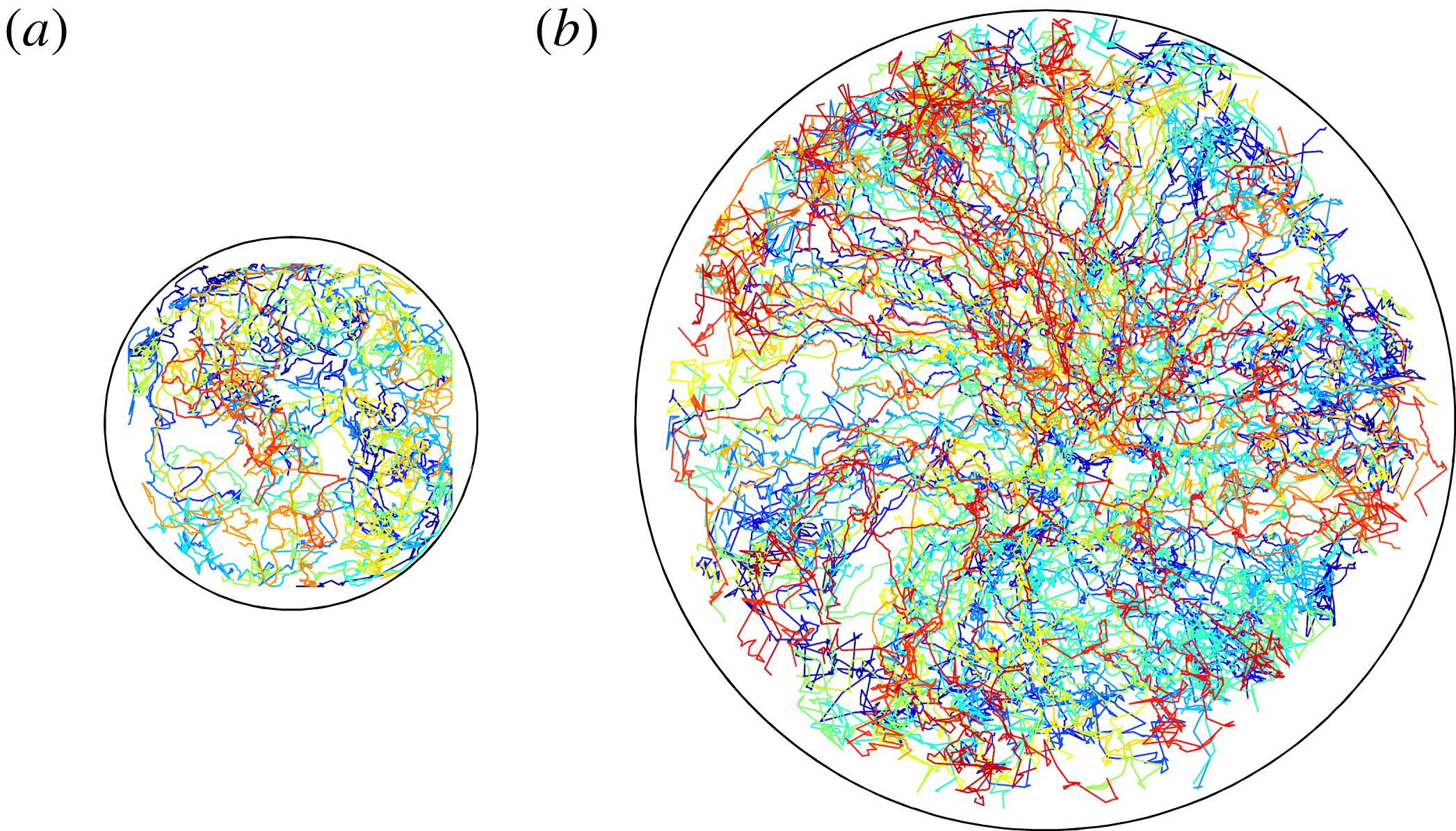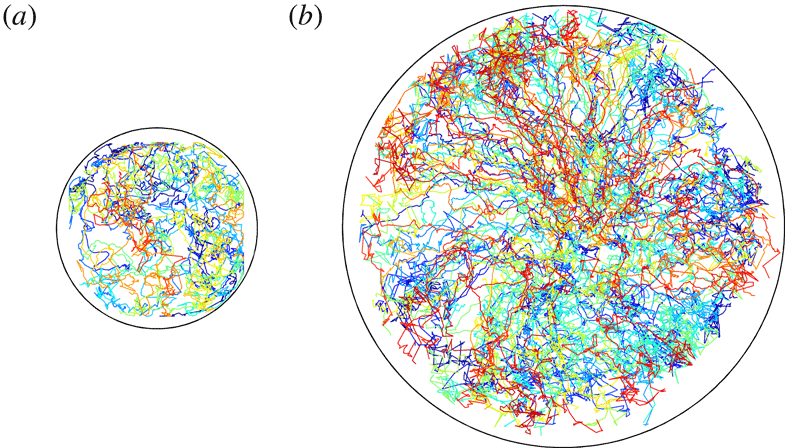With the larger vessel ( $\unicode[STIX]{x1D6E4}=4.75$ ) generating centrifugal force effects ( $Fr\sim 0.1$ ) from rapid rotations, such effects appear in the path lines for long times of presence $O(10^{2}~\text{s})$ (figure 16), and in figure 16, for clarity, only trajectories longer than $450~\text{s}$ are plotted. In figure 16(a), the vortex trajectories appear with repeated jerky movements, in the shape of random walks, and in figure 16(b) there are numerous trajectories that are largely directed radially outward. This radial motion is not straight, but features a zigzag pattern as the columns are strongly affected by their other surrounding vortices, as discussed earlier for figure 15. Columnar vortices in the large-aspect-ratio vessel behave as Brownian particles over short time scales $O(10^{0}{-}10^{1}~\text{s})$ , and are affected by centrifugal forces over longer time scales $O(10^{2}{-}10^{3}~\text{s})$ . As figure 11 also clearly shows, the influence of centrifugal forces on vortex motion appears only over the long time scales. To explain the details of this random-walk-like motion, a further discussion of its statistical nature will be given in the next section.

Figure 16.

Examples of path lines of columnar vortices persisting over 450 s with $Ta=1.0\times 10^{8}$ for (a)  $\unicode[STIX]{x1D6E4}=2.00$ and (b)  $\unicode[STIX]{x1D6E4}=4.75$ . Path lines are individually colour coded.

5.1 Horizontal diffusive motion of columnar vortices

Although the probability distributions of vortex advection speeds do not fit a purely Maxwell distribution with its classical assumptions, a random-walk-like motion, however, is observed in the path lines in figures 15 and 16. Based on this, there is the possibility that it will be possible to describe the vortex motion as diffusive motion. Brownian motion (random walk) shown by molecules in a thermal equilibrium state is one example of commonly occurring normal diffusive motion, natural diffusion without acceleration or deceleration. In other situations of turbulent diffusive arrangements, random Lagrangian particle motion can be represented as diffusive motion arising from macroscopic fluctuations (Solomon, Weeks & Swinney Reference Solomon, Weeks and Swinney1993). Diffusive motion is characterized by determining the mean-squared displacement (MSD):

(5.1) $$\begin{eqnarray}\text{MSD}=\langle \unicode[STIX]{x1D6FF}\boldsymbol{r}(t)^{2}\rangle =\frac{1}{N}\mathop{\sum }_{i=1}^{N}[\boldsymbol{r}_{i}(t)-\boldsymbol{r}_{i}(0)]^{2},\end{eqnarray}$$

where $\unicode[STIX]{x1D6FF}\boldsymbol{r}(t)$ is the displacement from the initial vortex position $\boldsymbol{r}(0)$ with time $t$ and angular brackets $\langle ~\rangle$ indicate an ensemble average. The time dependence of the MSD for normal diffusion processes is given by

(5.2) $$\begin{eqnarray}\langle \unicode[STIX]{x1D6FF}\boldsymbol{r}(t)^{2}\rangle \sim t^{\unicode[STIX]{x1D6FE}}\quad \text{with }\unicode[STIX]{x1D6FE}=1.\end{eqnarray}$$

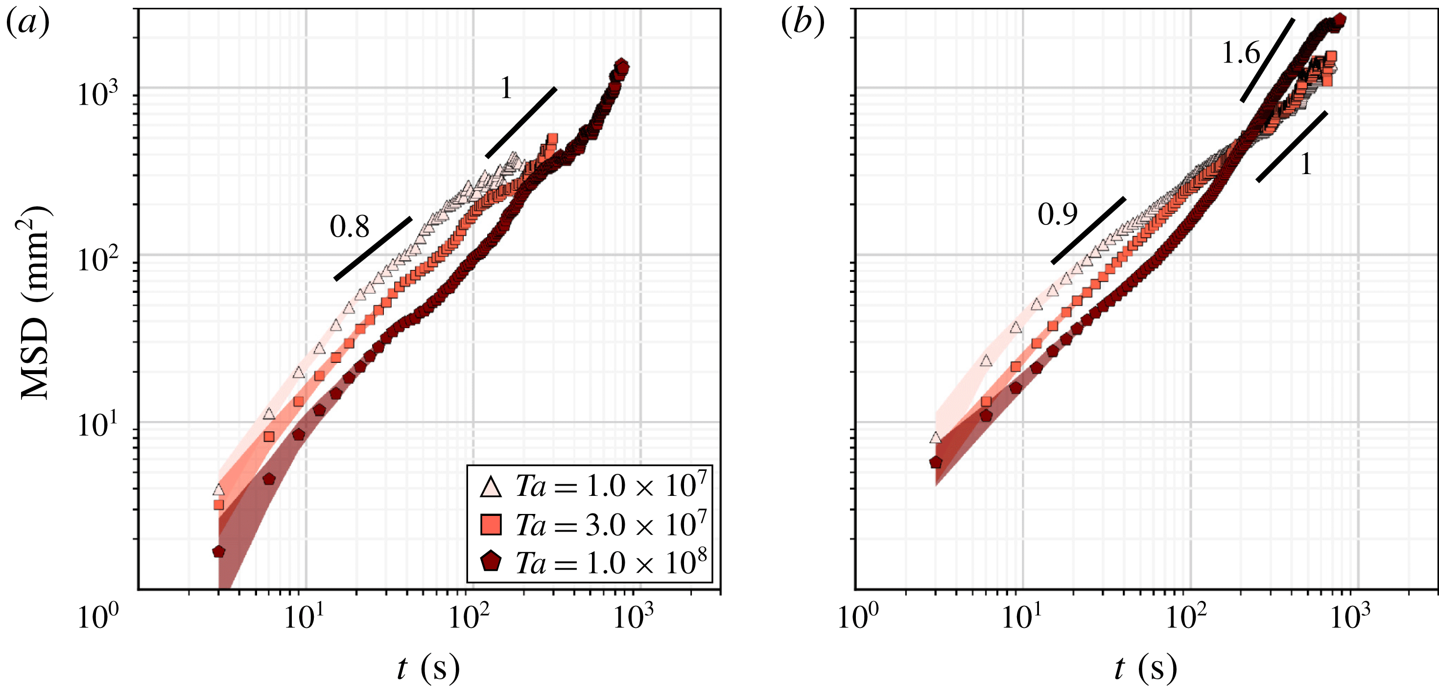
Instances of $\unicode[STIX]{x1D6FE}\neq 1$ indicate anomalous diffusion: super-diffusion ( $1<\unicode[STIX]{x1D6FE}<2$ ) influenced by acceleration and sub-diffusion ( $0<\unicode[STIX]{x1D6FE}<1$ ) influenced by deceleration. Diffusive motion commonly indicates the motion of very small molecules (particles). Meuel et al. (Reference Meuel, Prado, Seychelles, Bessafi and Kellay2012) performed an MSD analysis to investigate the motion of tropical cyclones, and quantification of diffusive motions of such macroscopic structures is also informative to understand the power sources and time scales dominating the motion. In the present study, an MSD analysis was applied to the horizontal motion of the columnar vortices to be able to discuss the complicated motion presently accepted as diffusive motion; the calculated MSDs are plotted in figure 17. To ensure the reliability of the statistics, only ensemble averages with more than 100 vortices are plotted in figure 17. This results in some discrepancy with the lifetimes shown in figure 14. The common feature to note in figure 17 is the relatively large MSD values appearing at low $Ta$ settings for both vessels with their different aspect ratios. The magnitude of the MSD reflects the speed of the diffusive motion of the columnar vortices, the speed of movements of the columns moving away from a specific position, the coefficient of diffusion $D(t)$ , which can be obtained from

(5.3) $$\begin{eqnarray}D(t)\equiv \frac{\langle \unicode[STIX]{x1D6FF}\boldsymbol{r}(t)^{2}\rangle }{2\unicode[STIX]{x0394}t}.\end{eqnarray}$$

Here, $\unicode[STIX]{x0394}t$ is the time interval of the vortex tracking; in the present case, $\unicode[STIX]{x0394}t=3~\text{s}$ . For both vessels, lower $Ta$ settings show larger $D(t)$ at $O(10^{0}{-}10^{2}~\text{s})$ . The calculated $D(t)$ are in the range of $10^{-7}{-}10^{-6}~\text{m}^{2}~\text{s}^{-1}$ , with the coefficient of viscous diffusion $\unicode[STIX]{x1D708}=1.0\times 10^{-6}~\text{m}^{2}~\text{s}^{-1}$ , and the coefficient of thermal diffusion $\unicode[STIX]{x1D705}=1.4\times 10^{-7}~\text{m}^{2}~\text{s}^{-1}$ . For the vessel with $\unicode[STIX]{x1D6E4}=2.00$ , $D(t)$ decreases as $Ta$ increases over the observed period. In addition to this $Ta$ dependence of the coefficient of diffusion, time variations in the slopes, $\unicode[STIX]{x1D6FE}>1$ in $O(10^{0}{-}10^{1}~\text{s})$ , $\unicode[STIX]{x1D6FE}<1$ in $O(10^{1}~\text{s})$ and $\unicode[STIX]{x1D6FE}\geqslant 1$ in $O(10^{1}{-}10^{2}~\text{s})$ , are also observed in the smaller vessel. However, for $\unicode[STIX]{x1D6E4}=4.75$ , there is no clear $Ta$ dependence, especially over long time scales. There are clear differences at the highest $Ta$ values in the larger vessel (filled pentagons in figure 17 b); the high $Ta$ MSD plots cross the two other lower $Ta$ conditions because of an abrupt increase in $\unicode[STIX]{x1D6FE}$ around $O(10^{2}~\text{s})$ , from $\unicode[STIX]{x1D6FE}\sim 1$ in $O(10^{1}~\text{s})$ to $\unicode[STIX]{x1D6FE}\sim 1.6$ in over $O(10^{2}~\text{s})$ . This difference appears only for the highest $Ta$ and may be ascribed to the effect of centrifugal forces. Centrifugal force accelerates the vortex motion in the radial direction, making the columnar vortices more easily diffuse and this results in the super-diffusive motion. Further, the intermediate time scale $O(10^{1}~\text{s})$ shows slight, but gradual decreases in $\unicode[STIX]{x1D6FE}$ for all settings. Viewing path lines drawn at the intermediate time scale (for 90 s) in figure 15, there is some regularity in the path lines, a result of the mutual interactions between adjacent vortices. This behaviour corresponds to a deceleration of the horizontal motion of the columnar vortices appearing as sub-diffusive motion, $\unicode[STIX]{x1D6FE}<1$ . Further discussion of this is provided below.

Figure 17.

The MSD $\langle \unicode[STIX]{x1D6FF}\boldsymbol{r}(t)^{2}\rangle$ of the horizontal motion of columnar vortices for different $Ta$ values with (a)  $\unicode[STIX]{x1D6E4}=2.00$ and (b)  $\unicode[STIX]{x1D6E4}=4.75$ . The numbers accompanying the black solid lines are the $\unicode[STIX]{x1D6FE}$ values. Faded-colour areas behind each plot indicate the standard deviation of the MSD.

5.2 Anomalous diffusion of columnar vortices

For the higher $Ta$ settings, a smooth MSD plot (figure 17) is obtained over time scales of $O({>}10^{2}~\text{s})$ as the number of long-lived vortices is large. It is however impossible to obtain smooth curves for the lower $Ta$ settings because the lifetimes of the columnar vortices are relatively short making it difficult to record a sufficiently large number of data points for ensemble averaging. With the slope of the MSD for $\unicode[STIX]{x1D6FE}\neq 1$ , the translational motion of the columnar vortices cannot be considered a pure normal diffusive motion like the random walk displayed by Brownian particles. In particular, as discussed at the end of § 5.1, intermediate time scales $O(10^{1}~\text{s})$ for $\unicode[STIX]{x1D6E4}=2.00$ and $Ta=1.0\times 10^{8}$ show slight decreases in $\unicode[STIX]{x1D6FE}$ to $\unicode[STIX]{x1D6FE}\sim 0.8{-}0.9$ . 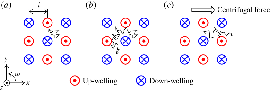For this setting, the vortex motion represented as the path lines in figure 15 is restricted by the adjacent vortices of opposite vorticities. The two types of down-welling and up-welling vortices do not merge, but assume a checkerboard (regular grid) pattern in the vortex arrangement. The random-walk-like motion of a down-welling vortex follows the patterns suggested by the arrow in figure 18(a). This may be interpreted to show that the vortex motion is enclosed by a barrier of different-type vortices at this intermediate time scale (figure 18 b).

To understand this anomaly in the diffusive vortex motion, the characteristics of columnar vortices different from Lagrangian particles must be considered because the columns are macroscopic flow structures, and are continuous phase to the ambient fluid. For instance, the size of the columnar vortices must be considered unlike negligibly small particles. In addition, columnar vortices have a wide range of lifetimes (observable lives). Depending on the time of observation (lifetime), the observed diffusive motion may vary as strong mutual interactions shown as regularities in figure 15. It may be that the relevant mutual interactions from the surroundings appear at the collision of one vortex with another, making it necessary to consider the mean free time $\unicode[STIX]{x1D70F}$ of the columnar vortices. In this case, $\unicode[STIX]{x1D70F}$ is the length of time between the collisions of one vortex and another and is given by $\unicode[STIX]{x1D70F}=l/v_{mp}$ , with $l$ the mean free distance. Assuming that columnar vortices fill the entire fluid layer, $l$ is equivalent to $L_{vortex}$ , and based on this the calculated $\unicode[STIX]{x1D70F}$ durations are listed in table 4.

Figure 18.

Conceptual diagram of the vortex motion without centrifugal force effects for (a)  $t_{life}<\unicode[STIX]{x1D70F}$ and (b)  $t_{life}\geqslant \unicode[STIX]{x1D70F}$ , and with centrifugal force effects for (c)  $t_{life}\gg \unicode[STIX]{x1D70F}$ .

Table 4.

Mean free time for columnar vortices for different $\unicode[STIX]{x1D6E4}$ and $Ta$ values.

For $t_{life}>\unicode[STIX]{x1D70F}$ , the vortex motion is affected by different adjacent vortices, as they repulse each other. As a result, the repulsions would yield an enclosure effect which slows the vortex motion and prevents unimpeded normal diffusive motion (figure 18 b). The mean free times $\unicode[STIX]{x1D70F}$ listed in table 4 indicate that such an effect appears at $O(10^{1}~\text{s})$ . From figure 17, the sub-diffusive trend, $\unicode[STIX]{x1D6FE}\sim 0.8{-}0.9$ , clearly reflects this effect, and the columnar vortices diffuse little over intermediate time scales.

Under conditions without the effect of centrifugal forces (or even negligibly small effects), there is no very large difference in $\unicode[STIX]{x1D70F}$ between the two vessels with different aspect ratios here. When centrifugal forces are working (at $Ta=1.0\times 10^{8}$ for $\unicode[STIX]{x1D6E4}=4.75$ ), $\unicode[STIX]{x1D70F}$ becomes shorter than that of $\unicode[STIX]{x1D6E4}=2.00$ because the horizontal motion is accelerated by this externally imposed force. The centrifugal forces move the down-welling vortices outward in the radial direction because the density of cold down-welling vortices is larger (figure 18 c). The up-welling vortices (lighter than the down-welling ones) are moved radially inwards in the vessel. Frequent collisions, which oppose free advection of columns towards each other, due to these radial accelerations are the reasons why $\unicode[STIX]{x1D70F}$ is shorter for the larger vessel than for the smaller vessel. In addition, for the larger vessel, the columnar vortex in the system undergoes super-diffusive motion due to the centrifugal forces over the long time scales $O({>}10^{2}~\text{s})$ . A large value of $\unicode[STIX]{x1D6FE}$ , $\unicode[STIX]{x1D6FE}\sim 1.6$ , as indicated in figure 17, supports this conclusion even though the mean free time $\unicode[STIX]{x1D70F}$ is shorter when a centrifugal force is working than when it is absent. The large value of $\unicode[STIX]{x1D6FE}$ for longer time scales $O({>}10^{2}~\text{s})$ observed in figure 17(b) with the highest $Ta$ value would be sustained or further enhanced for vessels of larger horizontal extent, and yield super-diffusive motion as in Lévy flights (e.g. Shlesinger, Zaslavsky & Klafter Reference Shlesinger, Zaslavsky and Klafter1993; Solomon et al. Reference Solomon, Weeks and Swinney1993), a repetition of stop–go motion. The value of $\unicode[STIX]{x1D6FE}$ asymptotes towards 2 indicating a ballistic diffusion if the experiment could be conducted in a vessel of infinite horizontal extent.

Columnar vortices are not completely isolated from their surroundings but are part of a continuous structure in the surrounding fluid as they are macroscopic flow structures as described above. Therefore, it is impossible to consider these as perfect rigid-body columns of tiny floating particles as discussed above. The unclearly delineated borders and variable body, which are easily affected by the surroundings, are the reasons why clear flight events are not observed. Merging events of the same type of vortices are also thought to be a reason. Commonly, a vortex is surrounded by two types of vortices with a somewhat loose regularity (figure 18). Vortices with opposite vertical flow directions repel each other, whereas the same types of vortices merge (e.g. Zhong et al. Reference Zhong, Ecke and Steinberg1993; Julien et al. Reference Julien, Legg, McWilliams and Werne1996; Pieri et al. Reference Pieri, Falasca, Hardenberg and Provenzale2016; Noto et al. Reference Noto, Tasaka, Yanagisawa, Park and Murai2018). Ideally, the probability that a vortex collides with either type of vortex is almost even for high $Ta$ values, because the populations of up-welling and down-welling vortices are almost the same (Vorobieff & Ecke Reference Vorobieff and Ecke2002; Sprague et al. Reference Sprague, Julien, Knobloch and Werne2006). Opposite-type vortices behave as a barrier preventing normal (random) diffusive motion. The geometric (quasi-polygonal) path lines (figure 15 c,f) are formed by this directivity because of the enclosure effect. Further, merging events do not affect the vortex motion and do not appear in the MSD analysis (figure 17), but only affect the lifetimes (figure 14). These various characteristics of the columnar vortices enable some balance resulting in the $\unicode[STIX]{x1D6FE}$ exponent close to unity.