Admittedly, the considered data are clustered at the national level, a fact which was not accounted for in Lundborg et al. (Reference Lundborg, Nystedt and Lindgren2007). Thus, reported BMI parameter estimates might be inefficient, i.e. reported standard errors might be too small. The coefficient estimates, however, would not be affected by such clustering, and we certainly note that the Schneider and Grimps estimate of the association between divorce rate and BMI within married couples (−3.25) closely mirrors the LNL estimate (−3.28). The estimated coefficient is still sizeable, implying for instance, that an increase in the divorce rate by 10 percentage points has the same effect on BMI as another 2–3 years of schooling.

In this response, we will first make some notes about the adequacy of applying multilevel methods to the data used by Lundborg et al. (Reference Lundborg, Nystedt and Lindgren2007). We will argue that such methods are not well suited to deal with clustering in the data used by Lundborg et al. (Reference Lundborg, Nystedt and Lindgren2007). We will then claim that some of the arguments used by Schneider and Grimps are flawed. This applies especially to their concluding argument that, ‘Only if singles have a lower BMI will there be an incentive for the married to slim.’ After that, we will show that the Schneider and Grimps results, based on multilevel techniques, are sensitive to outliers.

It is well known that multilevel (parametric) models rely on strong asymptotic distributional assumptions and, hence, are crucially dependent on a sufficient number of observational units at all levels of the analysis. In the data at hand there are only ten level-2 clusters (nations). There are no exact guidelines on the minimal number of clusters necessary for statistical inference using multilevel models, but apparently most references in the literature consider ten to be too small a number. As a rule of thumb, previous researchers have advocated that the number should at least exceed 30 or even 50 (see e.g. Hox, Reference Hox, Balderjahn, Mathar and Schader1998; Maas & Hox, Reference Hox, Balderjahn, Mathar and Schader2004, and references herein). Angrist & Pischke (Reference Angrist and Pischke2009) suggest a minimum of 42 clusters.

With too few clusters, estimates of variances and significance levels should be interpreted with utmost caution, although parameter estimates may still be unbiased. It is unfortunate that Schneider and Grimps, applying multilevel analysis to a data set with only ten level-2 clusters, fail to discuss or mention anything about these shortcomings. An additional problem of using multilevel models with too few clusters is that there is no straightforward or widely accepted method of accounting for a situation of too few clusters. For an instructive discussion, see, for instance, Angrist & Pischke (Reference Angrist and Pischke2009), pp. 319–323. Naturally, the problems of too few clusters are reinforced in the presence of outliers or influential observations at the second level. As shown below, there is, indeed, one of the nations under study, for which the association between divorce risk and BMI among the married diverges markedly from the estimated pattern, heavily influencing the estimated fit.

Beside the technical point about the application of multilevel models, our main objection to the Schneider and Grimps comment concerns their categorical and concluding argumentation regarding the incentives for married people to control their weight: ‘Only if singles have a lower BMI will there be an incentive for the married to slim.’ We fail to see the logic behind this claim – Schneider and Grimps make no attempt to qualify their argument – and, given the dynamics of the marriage market, their statement may not necessarily be true. If a slim body constitution is valued highly in the marriage market, selection processes may well leave large fractions of overweight and obese people unmarried. Though married people may gain weight during marriage, they could still weigh less on average than the unmarried. This does not mean, however, that they would not have incentives to stay prepared for divorce by controlling their BMI. Such incentives would exist, if there is a negative connection between BMI and attractiveness in the marriage market. Under such premises, divorce risk always constitutes a motive to stay slender within marriage, an incentive that becomes stronger the higher the risk. Therefore, in addition to being in essence false, the Schneider and Grimps claim is surprising given the ease by which it could be refuted. One just needs to report how the patterns of average BMI of both singles and married relate to the divorce risks in the considered countries, information that is obviously just a few mouse clicks away.

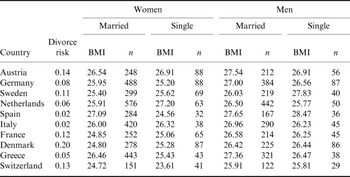
Therefore, in the following section, the association between average BMIs among married and singles is demonstrated and discussed. The relation between BMI levels and national divorce risks will be illustrated by simple figures and non-parametric correlations. The data are those used by Lundborg et al. (Reference Lundborg, Nystedt and Lindgren2007). The data will also be subdivided by gender. The reason is that previous research has indicated that a slender stature of a partner is more highly valued by men than by women, e.g. heavy women (but not men) are less likely to marry and when they do, they part up with partners of lower earnings than lean women (e.g. Gortmaker et al., Reference Gortmaker, Must, Perrin, Sobol and Dietz1993; Averett & Korenman, Reference Averett and Korenman1996). This indicates that an appropriate body constitution may yield higher returns in the marriage market for women than for men, which in turn implies that any incentives to stay slender within marriage may be greater for women, and that any connection between divorce risk and BMI among the married may be more apparent for women.

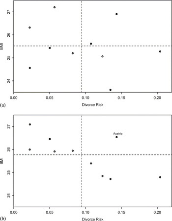
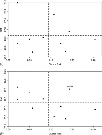
In Table 1, national divorce risks and average BMIs by gender and marital status are presented. The associations are visualized in Fig. 1 for women and in Fig. 2 for men. In all figures, the vertical dotted line depicts the average national divorce risk and the horizontal dotted line the mean of average BMI for the gender and marital status under study. This facilitates a fast and simple visual inspection as it subdivides the figures into four segments according to two dimensions: relative high/low BMI/divorce risk.

Fig. 1.

National divorce risk and average BMI among (a) single and (b) married women.

Fig. 2.

National divorce risk and average BMI among (a) single and (b) married men.

Table 1.

Divorce risks and average BMI for married and single men and women

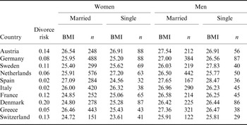
There is apparently no visually detectable association between BMI and divorce risk among single women (Fig. 1a). Among the five countries with relatively low divorce risk (to the left of the vertical line), three have low mean BMIs and two have high. The distribution of average BMIs is the same among the five high divorce risk countries.

On the other hand, the observations for married women expose a pattern where there is a rather stark discernable, almost linear negative association between BMI and divorce risk (Fig. 1b). The only observation that markedly deviates from this pattern, neither being classified as a high divorce risk/low BMI, nor a low divorce risk/high BMI country, is Austria, for which both average BMI and divorce risk are rather high.

A qualitatively similar picture was found for men. There is no apparent association between BMI and divorce risk among singles (Fig. 2a), while there is a generally negative relation between BMI and divorce risk for married men (Fig. 2b). The pattern is somewhat less evident than for women, though, and again, Austria diverges from the predicted pattern by being a high divorce risk/high BMI country. There is also an observation falling into the low divorce risk/low BMI category (Netherlands), though it fits rather well to the observed pattern of a negative relationship between divorce risk and BMI.

The limited number of observations (ten) on national average BMI and divorce risks does not lend itself to parametric estimations. However, Kendall's τ might be used. It constitutes a non-parametric correlation approach, based on whether the rankings of the respective entities (BMI and divorce risk) are concordant or disconcordant. According to this measure, there is a significant correlation between average BMI and divorce risk for married women (τ=−0.511, p=0.047), but not for single women (τ=−0.111, p=0.73). By the same token, no association between divorce risks and BMI among single men could be identified (τ=−0.022, p=1.00). For married men, the estimated association was weaker (τ=−0.333, p=0.22) than for married women. Though using a rather blunt technique and aggregate data, these results indicate that whereas there is no association between divorce risks and BMI among singles, there is a stronger association between divorce risk and BMI for married women than for men.

As shown above, visual inspection suggests that Austria constitutes an outlier in the sense that the association between divorce risk and average BMI diverges from the overall pattern among both married men and women. There is no inferential justification for excluding Austria from the analysis, though, since there are no indications of misreports or any other measurement errors in the Austrian figures. Nevertheless, we will demonstrate the sensitivity of multilevel analysis to a single influential observation at the second level, when there are just a few units at this level. Thus, we briefly present estimates of the influence of divorce risk on BMI among the married with and without the Austrian observations included. The estimated models correspond to the full models in Lundborg et al. (Reference Lundborg, Nystedt and Lindgren2007) and Schneider and Grimps, respectively, when it comes to included variables, though the account here is limited to the parameter estimates of the association between BMI and divorce risk (the remaining parameter estimates were highly similar to the ones presented in Lundborg et al. (Reference Lundborg, Nystedt and Lindgren2007)).

Formally the estimated random intercept model may be written as:

where the BMI of individual i in country j is a function of observed individual characteristics x_ij, divorce risk in country j (DR_j), a random effect varying between countries (u_j) and an individual-specific error term (e_ij), the last two both being independently and identically distributed. The models are estimated in STATA via the ‘xtmixed’ command using restricted maximum likelihood (REML). Results are presented in Table 2.

Table 2.

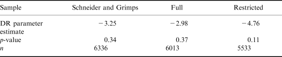
Illustration of sensitivity: multilevel estimation (Random Intercept) of the divorce risk (DR) influence on BMI among the married, from Schneider and Grimps, and with full and restricted sample (without outlier, Austria)

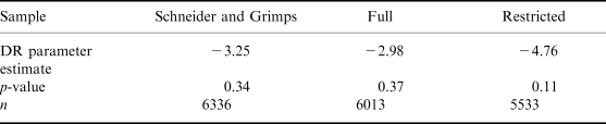
As shown in the first column of Table 2, Schneider and Grimps found a statistically insignificant effect of divorce risk on BMI among the married amounting to −3.25 (p=0.34). The estimated effect of one year of schooling on BMI was −0.14 (see Schneider & Grimps in this issue of JBS), an effect obtained also in both our multilevel specifications of Table 2 (results not shown). Taken literally, this implies that a 10 percentage point increase in divorce risk has a similar effect on BMI as 2.3 years of additional schooling, i.e. −0.325/−0.14=2.3. Our corresponding multilevel estimate of the divorce risk impact, using the full sample, is −2.98 (p=0.37, see Table 2, column 2), which by the same token is equivalent to 2.1 years of schooling. Note that there is a discrepancy in the reported number of observations (6013 here, and 6336 in Schneider and Grimps). We do not know the reason for this, if SAS (which is used by Schneider and Grimps) reports all observations regardless of whether they contain empty cells (contributes to the likelihood) or not, if we have used different versions of the SHARE data or if there are any other explanation. Nevertheless, the variation in the number of observation does not seem to be heavily influencing the estimations. Now, discarding the outlier (Austria) from the estimations inflates the estimated influence of divorce risk on BMI to 4.76 (p=0.11, see Table 2, column 3), and a 10 percentage point increase in divorce risk is now similar to a 3.4 years increase in schooling. Though it should again be stressed that the estimates of variances in these cases are highly unreliable, given the small number of clusters on the second level, these results illuminate the sensitivity of multilevel estimation, when the number of clusters are too small.

No doubt, multilevel analysis has many advantages as a statistical technique, but it is not ein Mädchen für alles. As all methods, it also has its limitations and boundaries for its appropriate use. Above we have shown a number of shortcomings as far as analysing the data used in Lundborg et al. (Reference Lundborg, Nystedt and Lindgren2007) is concerned. The Schneider and Grimps use of the technique in this case, and the conclusions drawn, are not convincing. We still claim that the statistical material at hand does, indeed, imply that divorce risk at the national level may well influence the weight of the married.

In conclusion, body weight is a complex function of genes, environment, behaviour and their interactions. Though data sources have become qualitatively more sophisticated, large parts of the individual variations in BMI are still unexplained. Nevertheless, the socioeconomic pattern of obesity and BMI in the general population of developed countries implies that there is a negative association between education and BMI, especially among women (Sobal & Stunkard, Reference Sobal and Stunkard1989; McLaren, Reference McLaren2007). Whether the risks among married individuals of becoming divorced in the future – once again being valued in the marriage market for their psychological and physiological traits – to some extent also may govern their behaviour within marriage, remains an open question. From a theoretical standpoint, it is easy to find behavioural arguments that married people have incentives to respond to variations in the risk of experiencing divorce. Though admittedly circumstantial, the empirical results presented here, as well as in our previous article (Lundborg et al., Reference Lundborg, Nystedt and Lindgren2007), point in the same direction. Divorce risks are associated with BMI for married but not for single people. The magnitude of the effect implies that a 10 percentage point increase in divorce risk has an influence on BMI similar to the influence of 2–3 years of additional schooling. Whether the indication of such an influence is relevant or not from a societal perspective is a matter of opinion. Further research is obviously needed. Studies based on longitudinal data, in which the weight development of individuals is recorded over time, would enable deeper analysis of the dynamic association between weight and the marital life course.