



1. Introduction
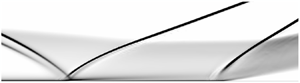
For a high-speed airbreathing propulsion system, the compression is performed through a series of oblique shocks, referred to as a shock train (Sullins & McLafferty Reference Sullins and Mclafferty1992). It plays a major role in decelerating the incoming flow and providing the necessary pressure rise for the downstream combustion. Understanding the dynamical properties of the shock train is critical for detecting and preventing inlet unstart because of its devastating effects on the engine performance (Wagner et al. Reference Wagner, Yuceil, Valdavia, Clemens and Dolling2009; Do et al. Reference Do, Im, Mungal and Cappelli2011b; Valdivia et al. Reference Valdivia, Yuceil, Wagner, Clemens and Dolling2014; Im & Do Reference Im and Do2018). Recently, the shock train has attracted much attention due to its unsteady behaviours (Laurence et al. Reference Laurence, Karl, Schramm and Hannemann2013; Im et al. Reference Im, Baccarella, McGann, Wermer and Do2016; Riley et al. Reference Riley, Gaitonde, Hagenmaier and Donbar2018; Hunt & Gamba Reference Hunt and Gamba2019).
One of the behaviours can be considered as a forced motion, which is dominated by extrinsic driving sources such as the backpressure (Klomparens, Driscoll & Gamba Reference Klomparens, Driscoll and Gamba2016; Su, Ji & Chen Reference Su, Ji and Chen2016). This unsteady motion can be explained by the fact that the shock train keeps changing its speed to match the varying backpressure by shifting the relative Mach number ahead of it (Bruce & Babinsky Reference Bruce and Babinsky2008; Xiong et al. Reference Xiong, Fan, Wang and Tao2018). Another mode is associated with the intrinsic dynamics of the shock train, which are self-excited fluctuations of the shock train about its time-averaged position even when both upstream and downstream conditions remain constant. The description of the shock train mechanism is further complicated by the presence of such behaviour, which was initially investigated by Ikui et al. (Reference Ikui, Matsuo, Nagai and Honjo1974) and confirmed by further studies (Matsuo et al. Reference Matsuo, Mochizuki, Miyazato and Gohya1993; Handa, Mitsuharu & Matsuo Reference Handa, Mitsuharu and Matsuo2005). The mechanism of this unsteady motion is also controversial. Yamane et al. (Reference Yamane, Kondo, Tomita and Sakae1984a) and Yamane, Takahashi & Saito (Reference Yamane, Takahashi and Saito1984b) conjectured that the oscillation is caused by the interaction of the disturbances that travel through opposite directions and excite each other, whereas Sugiyama et al. (Reference Sugiyama, Takeda, Zhang, Okuda and Yamagishi1988) suggested that the oscillation is caused by a throat-like shape in the shock train. Since the boundary layer thickness changes along the duct, the throat cross-section also changes and induces the first shock to oscillate.
To obtain the most basic characteristics of the shock train, most previous studies were performed in a relatively uniform flow field and they made great progress (Hutchins et al. Reference Hutchins, Akella, Clemens, Donbar and Gogineni2014; Im et al. Reference Im, Baccarella, McGann, Wermer and Do2016; Klomparens et al. Reference Klomparens, Driscoll and Gamba2016; Su et al. Reference Su, Ji and Chen2016; Vanstone et al. Reference Vanstone, Hashemi, Lingren, Akella, Clemens, Donbar and Gogineni2018; Vanstone, Lingren & Clemens Reference Vanstone, Lingren and Clemens2018; Xiong et al. Reference Xiong, Fan, Wang and Tao2018; Hunt & Gamba Reference Hunt and Gamba2019). However, the potential risks caused by complicating effects such as flow distortion and shock-wave–boundary-layer interaction (SWBLI), which can emerge in a real flight, cannot be identified in such studies. For a real intake system, the inherent oblique shocks reflected from compression surfaces result in an inevitable non-uniform flow field in the isolator, especially in the streamwise boundary layer. In this situation, the motion of the shock train changes in the vicinity of the SWBLI, and the unsteady movement of the shock train induced by the SWBLI emerges in a large amplitude, which is significantly enhanced compared with the self-excited oscillation (Wagner, Yuceil & Clemens Reference Wagner, Yuceil and Clemens2010; Tan, Sun & Huang Reference Tan, Sun and Huang2012). In some cases, even with a slight change in the backpressure, a rapid movement can also be observed (Li et al. Reference Li, Chang, Xu, Yu, Bao and Song2017; Huang et al. Reference Huang, Tan, Sun and Wang2018), during which the shock train leading edge (STLE) passes through the SWBLI region quickly and stabilizes upstream. This phenomenon may pose a threat to the safety of the engine. In particular, when the shock train approaches the isolator entrance, the rapid forward movement may lead to inlet buzz or unstart. Owing to the severely detrimental effects of inlet unstart on the scramjet performance, many of the studies that intend to control inlet unstart focused on controlling the shock train position (Donbar Reference Donbar2012; Ashley et al. Reference Ashley, Szmuk, Clemens, Akella, Gogineni and Donbar2014; Valdivia et al. Reference Valdivia, Yuceil, Wagner, Clemens and Dolling2014; Vanstone et al. Reference Vanstone, Hashemi, Lingren, Akella, Clemens, Donbar and Gogineni2018), which can effectively suppress inlet unstart before its onset. However, the unstable motion caused by the SWBLI region may bring difficulty for shock train detection and location control. Although a successful closed-loop control has been implemented (Valdivia et al. Reference Valdivia, Yuceil, Wagner, Clemens and Dolling2014; Vanstone et al. Reference Vanstone, Hashemi, Lingren, Akella, Clemens, Donbar and Gogineni2018), the applicability of the control scheme to a highly distorted inlet, in which the shock train location is nonlinear, is still uncertain (Wagner et al. Reference Wagner, Yuceil and Clemens2010; Tan et al. Reference Tan, Sun and Huang2012; Wang et al. Reference Wang, Cheng, Cheng and Xue2018). Therefore, before developing a control scheme, the characteristics of the shock train, especially considering the effects of the SWBLI, should be analysed first.
The focus of this study is to investigate the formation mechanism of the unsteady motion caused by the SWBLI, because once this mechanism is revealed, an appropriate control scheme can also be developed. If the unsteady movement is induced by external excitation, such as unsteadiness in the incoming flow, the shock train can be stabilized by eliminating the source. However, if the unsteady movement is caused by the intrinsic dynamics of the shock train, we should consider how to enhance the system stability. Flow control (bleeding or ejecting) and feedback control are two usual approaches applied in isolators for resisting the shock train. Flow control can suppress the unstable movement by modifying the intrinsic dynamics of the shock train to attain stability. By understanding the relationship between the flow condition and the shock train motion, we can design a more effective control method. With a proper controller, the closed-loop control method has the ability to suppress perturbations by feeding back the deviation (MacMartin Reference MacMartin2004). Valdivia et al. (Reference Valdivia, Yuceil, Wagner, Clemens and Dolling2014) attempted to arrest inlet unstart by vortex generator jets. However, this type of active control is challenging due to the rapid actuation time required. The closed-loop control system can prevent unstart approximately  $50\,\%$ of the time. Thus, the capability of the actuator to dominate the shock train motion (controllability) should be analysed. To suppress perturbations using a closed-loop control system, the deviation needs to be measured and fed back to the controller. Then, it is also necessary to clarify how well the shock train movement can be inferred by the monitored signal (observability). However, only few studies have focused on these issues such that it is still unknown which flow parameter is responsible for the instability and whether the actuator is capable of dominating the shock train in this situation.
A previously developed shock train model (Li et al. Reference Li, Chang, Xu, Yu, Bao and Song2017) has motivated us to investigate the intrinsic dynamics of the shock train by means of a linear stability analysis. In this study, the Smart–Ortwerth model described by Smart (Reference Smart2015) was utilized to obtain the equilibrium state of the shock train, and at this equilibrium state, linearization was performed to obtain the state-space form of the shock train model. Then, the dynamical properties of the shock train system were revealed during the process of passing through the SWBLI region. The relationship between the key parameter in the boundary layer and shock train stability was deduced theoretically based on the free-interaction theory. Because the rapid movement poses a greater potential threat than oscillations, the formation of these two unstable movements was analysed further based on the limit cycle theory. Based on the state-space model, a controllability analysis was conducted to analyse the ability of the actuator to dominate the shock train motion. In practice, the shock train location cannot be directly measured; thus, an estimation of the location using the monitored signal that can be treated as the output of the shock train system is required to feed back to the controller. We constructed an expression for the output energy, and with a singular value decomposition, the contribution of the shock train motion to the output was obtained. Based on this analysis, a better approach for shock train detection was confirmed theoretically, and some phenomena observed in previous studies were also explained. These aspects are the key findings of this investigation, which can provide a basis for shock train control.
The structure of the paper is as follows. In § 2, the shock train model and its linearization are presented. Section 3 describes the linear stability analysis, which is necessary to confirm if the shock train unsteady movement induced by the SWBLI is caused by its intrinsic dynamics. In § 4, we present the analysis of the key parameter responsible for the intrinsic dynamics and its effects. After analysing the cause of the unsteady movement, the control strategy is subsequently discussed. In § 5, we provide the controllability and observability analyses and, finally, the concluding remarks are given in § 6.
2. Problem description and model equations
2.1. Statement of the problem
According to previous investigations (Tan et al. Reference Tan, Sun and Huang2012; Li et al. Reference Li, Chang, Xu, Yu, Bao and Song2017; Huang et al. Reference Huang, Tan, Sun and Wang2018), the shock train behaviour is closely associated with the boundary layer condition. The disturbance due to the SWBLI makes the boundary layer thicken or separate intermittently along the tunnel, which leads to different shock train behaviours. Thus, the problem is essentially how a moving shock train behaves in the SWBLI region. To define the problem, consider the interaction in the schematic shown in figure 1. In practice, the flow field in the isolator is complex, involving perturbations induced from the incoming flow and combustion. Thus, it is difficult to establish a fundamental understanding of the interaction between the shock train and the SWBLI. To simplify this investigation, the movement of the shock train is considered to be driven by a throttle device that induces little perturbation and is widely used in the study of shock trains (Hutchins et al. Reference Hutchins, Akella, Clemens, Donbar and Gogineni2014; Klomparens et al. Reference Klomparens, Driscoll and Gamba2016; Huang et al. Reference Huang, Tan, Sun and Wang2018; Vanstone et al. Reference Vanstone, Hashemi, Lingren, Akella, Clemens, Donbar and Gogineni2018; Xiong et al. Reference Xiong, Fan, Wang and Tao2018; Hunt & Gamba Reference Hunt and Gamba2019).
Schematic of the problem domain.

Actually, the SWBLI is three-dimensional (3-D), and its effects have been investigated widely (Bruce et al. Reference Bruce, Burton, Titchener and Babinsky2011; Burton & Babinsky Reference Burton and Babinsky2012; Clemens & Narayanaswamy Reference Clemens and Narayanaswamy2014; Grossman & Bruce Reference Grossman and Bruce2018). In the SWBLI region, a primarily reverse flow zone exists in the centre of the channel and two tiny corner reverse flow zones are located separately close to the sidewalls. The corner separation results in the formation of compression waves at the corner. These compression waves interact with the leading leg of the primary shock to constitute an intermediate zone. In the intermediate zone, compression waves from the corner separation lead to a more gradual deceleration and gentler adverse pressure gradient. Consequently, the boundary layer does not separate in this area (see figure 20 of Burton & Babinsky (Reference Burton and Babinsky2012)). Compared with the central separation, the corner separation has less impact. In addition, according to the findings of Wang et al. (Reference Wang, Sandham, Hu and Liu2015), the separation line is straight over the central part of the channel, while the reattachment line is curved, making the separation length in the streamwise direction near the centreline longer. For a large aspect ratio, the central interaction zone is relatively two-dimensional (2-D) and the size is increased; in contrast, the effects of the zones in the corner are weakened (see figure 8 of Wang et al. (Reference Wang, Sandham, Hu and Liu2015)). The unstable movements of the shock train observed by Tan et al. (Reference Tan, Sun and Huang2012) and Huang et al. (Reference Huang, Tan, Sun and Wang2018), of which the aspect ratios satisfy the condition mentioned by Wang et al. (Reference Wang, Sandham, Hu and Liu2015), can also confirm this. Furthermore, in the investigation by Xu et al. (Reference Xu, Chang, Zhou and Yu2015), the unsteady shock train motion in the SWBLI region was presented by a 2-D numerical simulation in the absence of corner and sidewall effects. Based on the analyses above, it is reasonable to infer that the unsteady behaviour of the shock train in such case can be triggered by a 2-D interaction alone, and the 3-D effects will be ignored in the following analysis.
2.2. Shock train modelling
The question here is how to investigate the dynamical mechanism and criterion of the unsteady shock train movement in the isolator. The key to answering this question is to construct an appropriate fluid model for the shock train. Currently, the widely used computational fluid dynamics model is nonlinear and of high order. It can help display the details of the flow structures but it is not convenient for analysing the mechanism and criterion of the unsteady motion. Therefore, the premise in the study of the unsteady mechanism is to set up a low-order model, which has an advantage of distinctly displaying the physical mechanism associated with stability. In this section, the problem is further reduced to one-dimensional.
Some analytical models have been proposed to analyse the dynamics of a normal shock (Culick & Rogers Reference Culick and Rogers1983; MacMartin Reference MacMartin2004; Bruce & Babinsky Reference Bruce and Babinsky2008). For a shock train, which is more complex, some studies have attempted to actively predict the shock train location using system identification (Hutchins et al. Reference Hutchins, Akella, Clemens, Donbar and Gogineni2014; Vanstone et al. Reference Vanstone, Hashemi, Lingren, Akella, Clemens, Donbar and Gogineni2018). The system identification requires no knowledge of the shock train physics; however, a simple physics-based model was then developed (Vanstone et al. Reference Vanstone, Lingren and Clemens2018). Xiong et al. (Reference Xiong, Fan, Wang and Tao2018) proposed a correlation with high precision between the amplitude of the shock train motion and the flow parameters. Unfortunately, these shock train models may be not suitable for analysing the dynamical properties of the shock train, as the coupling between the upstream and downstream flow is ignored. The air column between the first shock and the duct exit also plays a role in the transient behaviour (Sugiyama et al. Reference Sugiyama, Takeda, Zhang, Okuda and Yamagishi1988). When the first separation shock moves forward, the flow in the shock train region will be reconstructed transiently. This perturbation has an impact on the flow condition at the throat in the flap region, and then the flow at the throat affects the entire shock train, making a feedback system.
We begin by stating the governing equations for the shock train. A detailed derivation of these equations has been presented by Li et al. (Reference Li, Chang, Xu, Yu, Bao and Song2017), in which the suitability of the model was examined experimentally and numerically. The difference is that minor modifications were made to the model in this study to achieve a better fit. The model assumptions are as follows: (a) ideal gas and inviscid flow assumptions with a constant ratio of specific heat  $\gamma$ and gas constant
 $R$, but the skin friction coefficient, which is associated with the SWBLI, is considered; (b) quasi-one-dimensional flow; (c) the unsteadiness phenomena in the incoming flow and shock train region are not considered; and (d) the heat release due to combustion is ignored. To simplify the modelling, the motion of the first separation shock is also assumed to represent the entire shock train behaviour. Due to the limited information obtained from the experiment, the approximate parameters of the experimental flow fields are obtained by 2-D numerical simulations and are used to assist the modelling. The free interaction theory, which states the pressure rise behind the separation shock (Chapman, Kuhen & Larson Reference Chapman, Kuhen and Larson1957), is introduced to relate the upstream and downstream conditions as follows:
 \begin{equation} \frac{p_2-p_1}{q_1} \propto \sqrt{\frac{2C_{f1}}{({M_1}^2-1)^{0.5}}}, \end{equation}
where  $p$ is the wall pressure,
 $q$ is the dynamic pressure,
 ${C_f}$ is the skin friction coefficient,
 $M$ is the Mach number and the subscripts ‘1’ and ‘2’ denote the upstream and downstream conditions of the first separation shock, respectively. Because the wall pressure is highly nonlinear, we use
 ${0.5 \gamma p_{\infty }{M_1}^2}$ to approximate the dynamic pressure
 $q_1$. Considering that the Mach number in the current case is larger than 1.5, we approximate
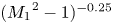 $({M_1}^2 - 1)^{-0.25}$ to
 ${{M_1}^{-0.5}}$ to simplify the calculation. On the other hand, for a moving shock at a velocity with respect to the channel,
 ${M_1}$ is replaced by
 $(u_1-\dot {x}_{{s}})/{a_1}$ (Culick & Rogers Reference Culick and Rogers1983), where
 $u$ is the velocity of flow,
 ${x}_{{s}}$ is the location of the STLE and
 $a$ is the speed of sound. Then we have
 \begin{equation} \frac{p_2-p_1}{p_{\infty}} = \frac{\gamma}{2}F\left(\frac{u_1-\dot{x}_{{s}}}{a_1}\right)^{1.5}\sqrt{2C_{f1}}, \end{equation}
where  ${F}$ is a universal correlation function that is independent of Mach and Reynolds numbers (Chapman et al. Reference Chapman, Kuhen and Larson1957; Matheis & Hickel Reference Matheis and Hickel2015). It can be used to approximate the wall pressure evolution for a given Mach number and friction coefficient once
 ${F}$ has been determined by experiments or numerical simulations. For turbulent flow, a value of
 ${F} = 7.5$ produces a better agreement with the current experimental results (Li et al. Reference Li, Chang, Xu, Yu, Bao and Song2017).
A simple first-order transient response model (Cui, Wang & Yu Reference Cui, Wang and Yu2014) is used to describe the variation of the pressure behind the first separation shock  ${p_2}$, which is given by
 \begin{equation} \dot{p}_2 = -\frac{p_2-{{\mathcal{P}}(x_{{s}}, p_{{b}})}}{\tau}, \end{equation}
where the subscript ‘ $b$’ denotes the flow condition at the exit. The propagation time constant
 $\tau$ is calculated as
 $(x_{{b}}-x_{{s}})/a_2$ and the location of the throat
 $x_{{b}}$ is 0.46. Here,
 $\mathcal{P}(x_{{s}}, p_{{b}})$ is a function to obtain the pressure behind the first separation shock when the backpressure
 $p_{{b}}$ is disturbed (see Li et al. (Reference Li, Chang, Xu, Yu, Bao and Song2017), p. 8).
The coupling between the upstream and downstream flow, namely the duct volume effect, is described as follows:
 \begin{equation} \dot{m}_{\infty} - \dot{m}_{b} = \frac{\mathrm{d} {\rho_{b} V}}{\mathrm{d} t} = V\dot{\rho}_{b} + \rho_{b}\dot{V},\end{equation}
where  $\dot {m}$ is the mass flow rate. The rate of the density variation at the exit
 $\dot {\rho }_{b}$ is calculated as
 $(\rho _{b}\dot {p}_{b}) / (\gamma p_{b})$ according to the equation of state, and the volume of the region downstream of the shock train
 $V$ is described as
 $A(x_{{b}}-x_{{s}})$ where
 $A$ is the duct area. The density of the separated flow is difficult to obtain in the modelling and the flow has a low velocity in this region, thus, we use the lumped parameter at the exit instead.
According to the equations above, the dynamic features of the shock train are solved based on its equilibrium states with different backpressures. In the shock train, the core flow is supersonic whereas the separation flow is subsonic. It is difficult to estimate the steady-state relationship between the upstream and downstream conditions. Thus, the Smart–Ortwerth model is employed. Heat release and loss are ignored, and then the simultaneous ordinary differential equations can be described as
 \begin{gather} \frac{\mathrm{d} {M^2}}{\mathrm{d} (x/D_{{H}})} = -{M^2}\left(1+\frac{\gamma-1}{2}{M^2}\right) \left[\left(\frac{2}{{\gamma}p{M^2}}\frac{A}{A_{{c}}}\right)\frac{\mathrm{d} {p}}{\mathrm{d} (x/D_{{H}})}+ \left(4C_{f2}\frac{A}{A_{{c}}}\right)\right], \end{gather}
 \begin{gather}\frac{\mathrm{d} ({{A_{{c}}}/A})}{\mathrm{d} (x/D_{{H}})} = \left[\frac{1-{M^2}(1-{\gamma}(1-{A_{{c}}}/A))}{{\gamma}p{M^2}}\right] \frac{\mathrm{d} {p}}{\mathrm{d} (x/D_{{H}})}+\left(\frac{1+({\gamma}-1){M^2}}{2}\right)4C_{f2}, \end{gather}
 \begin{gather}\frac{\mathrm{d} {p}}{\mathrm{d} (x/D_{{H}})} = kC_{f\infty}\left(0.5{\gamma}p{M^2}\right), \end{gather}
where  $A/A_c$ and
 $D_{{H}}$ are the normalized core flow area and hydraulic diameter, respectively. Here,
 $C_{f2}$, which represents the skin friction at the wall in the entire separated region, is assumed to be zero,
 $k$ is an empirical constant. According to a previous finding (see figure 8 of Li et al. (Reference Li, Chang, Xu, Yu, Bao and Song2017)), the pressure gradient in the shock train region described by (2.5c) is set as constant. The function
 $\mathcal{P}(x_{{s}}, p_{{b}})$ can be obtained by solving (2.5) with initial conditions,
 $p_1(x_{{s}})$,
 $M_1(x_{{s}})$,
 $A / A_{{c}}$ and terminal condition
 $p_{{b}}$.
Combined with the disturbance propagation model, duct volume effect and the equilibrium manifold linearization approach used by Cui et al. (Reference Cui, Wang and Yu2014), the equations describing the dynamics of the shock train motion can be concluded as follows:
 \begin{gather} \dot{x}_{{s}} = - \frac{4\bar{a}_1(x_{{s}})}{3F{\gamma}p_{\infty}\sqrt{2\bar{M}_1(x_{{s}})\bar{C}_{f1}(x_{{s}})}} \left[p_2-\bar{p}_2(x_{{s}})\right], \end{gather}
 \begin{gather}\dot{p}_2 = -\frac{\bar{a}_2(x_{{s}})}{x_{{b}}-x_{{s}}}\left[p_2-\mathcal{P}({x}_{{s}}, p_{{b}})\right], \end{gather}
 \begin{gather}\dot{p}_{{b}} = -\frac{{\gamma}RT_{{t}}}{V\left[1+0.5({\gamma}-1){\bar{M}_{{b}}}^2\right]} \left[\dot{m}_{{b}}-\dot{m}_{\infty}\right]-\frac{{\gamma}{p}_{{b}}}{V}\dot{V}, \end{gather}
where ‘  $\bar { }$ ’ denotes the steady-state parameter. The speed of sound
 $\bar {a}_1$ and
 $\bar {a}_2$ are calculated with the static temperature of the incoming flow
 $T_{\infty }$ and the total temperature
 $T_{{t}}$, respectively. The distributions of
 $C_{f1}(x)$,
 $p_1(x)$ and the area-averaged Mach number
 $M_1(x)$ of the unthrottled flow are obtained in advance by a 2-D numerical simulation to assist the modelling, and the remaining parameters are solved by analytic expressions. Different from the previous work, the throttling ratio
 $A_{{b}} / A$ in the mass equation of (2.6c) is set as the input of the shock train system, and
 $p_{\infty }$ is used in the calculation instead of
 $p_1$ except for solving the ordinary differential equations. The validation of the shock train model is shown in appendix A.
2.3. Linearization of the shock train model
The dynamics equations (2.6) govern the evolution of the system state  ${\boldsymbol{\mathsf{X}}} = [x_{{s}} \enspace p_2 \enspace p_{{b}}]^{\text {T}}$. Then, the equations can be written in the form
 \begin{equation} \dot{{\boldsymbol{\mathsf{X}}}} = \mathcal{J}({\boldsymbol{\mathsf{X}}}, t). \end{equation}
The linear stability analysis assumes the existence of an equilibrium solution  ${\boldsymbol{\mathsf{X}}}_0$ for the system (2.6) referred to as the base flow and defined by
 $\mathcal{J}({\boldsymbol{\mathsf{X}}}_0) = 0$. Using the standard small perturbation technique, the instantaneous flow is decomposed into base flow and small disturbances
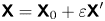 ${\boldsymbol{\mathsf{X}}} = {\boldsymbol{\mathsf{X}}}_0 + \varepsilon {{\boldsymbol{\mathsf{X}}}}^\prime$, where
 $\varepsilon \ll 1$. The resulting equations are further simplified by considering that the perturbation is infinitesimal, allowing the nonlinear fluctuating terms to be neglected. Thus, the nonlinear dynamic equations (2.6) become a system of linear partial differential equations defined by
 \begin{equation} \dot{{\boldsymbol{\mathsf{X}}}}^\prime = {\boldsymbol{\mathsf{A}}}{{\boldsymbol{\mathsf{X}}}}^\prime, \end{equation}
where the vector  ${{\boldsymbol{\mathsf{X}}}}^\prime =[{x_{{s}}}^\prime \enspace {p_2}^\prime \enspace {p_{{b}}}^\prime ]^{\text {T}}$ represents the perturbation variables. Here,
 ${\boldsymbol{\mathsf{A}}} = {{\mathrm {d} \mathcal{J}}/{\mathrm {d}{\boldsymbol{\mathsf{X}}}}}|_{{\boldsymbol{\mathsf{X}}}_0}$ is the Jacobian matrix obtained by linearizing the function
 $\textrm {Re}$ around the base flow
 ${\boldsymbol{\mathsf{X}}}_0$. To obtain the matrix
 ${\boldsymbol{\mathsf{A}}}$, we set
 ${{\boldsymbol{\mathsf{X}}}}^\prime = [{x_{{s}}}^\prime \enspace 0 \enspace 0]^{\text {T}}$ at
 ${\boldsymbol{\mathsf{X}}}_0$. Then we have
 \begin{equation} \dot{{\boldsymbol{\mathsf{X}}}}^\prime = {\boldsymbol{\mathsf{A}}}{{\boldsymbol{\mathsf{X}}}}^\prime = {\boldsymbol{\mathsf{A}}}\left[{x_{{s}}}^\prime \quad 0 \quad 0\right]^{\text{T}} = \frac{\mathcal{J}\left({{\boldsymbol{\mathsf{X}}}_0} + \varepsilon{{\boldsymbol{\mathsf{X}}}}^\prime\right) - \mathcal{J}\left({{\boldsymbol{\mathsf{X}}}_0}\right)}{\varepsilon}, \end{equation}
and the first column of the Jacobian matrix  ${\boldsymbol{\mathsf{A}}}$ is given by
 \begin{equation} \left[a_{11} \quad a_{21} \quad a_{31}\right]^{\text{T}} = \frac{\mathcal{J}\left({{\boldsymbol{\mathsf{X}}}_0} + \varepsilon{{\boldsymbol{\mathsf{X}}}}^\prime\right) - \mathcal{J}\left({{\boldsymbol{\mathsf{X}}}_0}\right)}{\varepsilon{x_{{s}}}^\prime}. \end{equation}
Similarly, we obtain the other two columns by setting  ${{\boldsymbol{\mathsf{X}}}}^\prime = [0 \enspace {p_2}^\prime \enspace 0]^{\text {T}}$ and
 ${{\boldsymbol{\mathsf{X}}}}^\prime = [0 \enspace 0 \enspace {p_{{b}}}^\prime ]^{\text {T}}$ at the same equilibrium point. Then, the eigenvalue of the linearized system
 $\lambda = \sigma + \omega {\textrm {i}}$ is also obtained at this equilibrium point. The sign of the leading eigenvalue's real part
 $\sigma$ determines whether the equilibrium solution is linearly stable or unstable, whereas its imaginary part
 $\omega$ characterizes the stationary or oscillatory nature of the associated eigenvector.
3. Mechanism of the unsteady movement induced by SWBLI
Similar to the self-excited oscillation, the significant unsteady movement of the shock train in the SWBLI region tends to be caused by the intrinsic dynamics of the shock train system due to the constant upstream condition and the slowly varying downstream condition. Based on the surrogate model developed in § 2, we performed a linear stability analysis of the shock train system during the process of passing through the SWBLI region, which is discussed in the following.
3.1. Characteristics of the unsteady shock train movement
We took the flow conditions in the study by Li et al. (Reference Li, Chang, Xu, Yu, Bao and Song2017) as examples to present the characteristics of the unsteady movement of the shock train. Tests were conducted at Mach 1.85 and 2.70 and the stagnation pressures were 0.215 and  $0.462\ \textrm {MPa} \pm 0.5\,\%$, respectively. The stagnation temperature was
 $305 \pm 5$ K. The thickness of the boundary layer at the exit of the wind tunnel was approximately 3.9 mm. This wind tunnel had an isolator test section that measures
 $50\ \text {mm wide} \times 30\ \text {mm tall} \times 320$ mm long. Fused silica windows were placed in the test section sidewalls for an optical access that measures
 $30\ \text {mm tall} \times 260\ \text {mm long}$.
In figure 2, the modelled trajectories are compared with the experimental ones. At a lower Mach number, as shown in figure 2(a), the model can predict the trend of STLE movement in general. According to the trajectory obtained from schlieren images, the oscillation emerges when the STLE enters the SWBLI region. For a higher Mach number, as shown in figure 2(b), a rapid forward movement is observed instead of the oscillation. Both the locations and moments when the unsteady motions occur in the model results are close to the experimental ones. It should be noted that the oscillation and rapid forward movement in different conditions are also distinguished by the model. The  $\lambda$-type shock train occurs at a lower Mach number and the pressure increases quickly in the front part. Accordingly, a larger slope was used in (2.5c). In contrast, for the case with a higher Mach number, the shock train has a
 $\chi$-type structure and the pressure rise is more gradual. Thus, a smaller slope was used in (2.5c) during the modelling.
The STLE trajectories at the bottom wall: (a) at  $M_{\infty } = 1.85$, the values of
 ${0.5\gamma pM^2}$ and
 ${kC_f}$ in (2.5c) are assumed to be 85.0 kPa and 0.35 during the modelling and (b) at
 $M_{\infty } = 2.70$, the values of
 ${0.5\gamma pM^2}$ and
 ${kC_f}$ in (2.5c) are assumed to be 111.4 kPa and 0.16. The location is normalized with the isolator length
 $L_{{iso}}$ and the time is normalized with
 $L_{{iso}} / u_{\infty }$. The data are selected from the experimental results of Li et al. (Reference Li, Chang, Xu, Yu, Bao and Song2017). The entire movements of the STLEs at
 $M_{\infty } = 1.85$ and
 $M_{\infty } = 2.70$ can be seen in the supplementary movies 1 and 2 available at https://doi.org/10.1017/jfm.2020.702.

Due to the assumptions in the modelling, this shock train model has some shortcomings, which are embodied in the following aspects. The coefficient  $k$ in the model may be unsuitable for other situations, due to the strong dependence on the flow conditions. Setting the coefficient as a constant may not be suitable for all cases. A data set or fitting function of
 $k$ obtained according to different flow conditions may give better performance, but numerous experimental data are required to support this process. Due to the dimensionality reduction in the modelling and simplification of the flow conditions, the modelled unsteady process lasts for less time than the experimental one. By using lumped parameters, which were obtained from a 2-D numerical simulation, parts of the effects of the SWBLI may be distorted. There exists a coupling between the movements of the STLEs at the lower and upper walls, however, this coupling is not modelled here, which also contributes to the disagreement. Nevertheless, the model presents the dynamic characteristics of the shock train within the SWBLI region and is considered to perform well considering the difficulty of mechanism modelling.
3.2. Linear stability analysis of the shock train movement
The time-domain behaviour suggests that there exists an instability mechanism inside the STLE movement. For a more detailed analysis, we focused on the linear stability analysis of the shock train behaviour. Figure 3 illustrates the details of the STLE movements in the second region of figure 2(a) and first region of figure 2(b). At the onset of the interaction between the STLE and SWBLI, the STLE oscillates with an increasing amplitude, which can be seen both in the model and experimental results. At a lower Mach number, the oscillation lasts until the STLE passes through the SWBLI region, of which the duration is approximately 0.300 s; whereas a rapid forward movement occurs instead at a higher Mach number and the duration is approximately 0.024 s. After the STLE crosses the SWBLI region, the decreasing amplitude of the oscillation suggests a decay process. According to the linearized equation set, at each equilibrium point, the Jacobian matrix  ${{\boldsymbol{\mathsf{A}}}}$ has one purely real eigenvalue and a pair of conjugate eigenvalues. This suggests that when the STLE is perturbed, it moves to a new position with a decaying oscillatory path as shown in the enlarged view of figure 3, which is consistent with the experimental results of Vanstone et al. (Reference Vanstone, Hashemi, Lingren, Akella, Clemens, Donbar and Gogineni2018).
Distributions of the flow parameters at the bottom wall and details of the STLE motions within the SWBLI regions: (a)  $M_{\infty } = 1.85$ and (b)
 $M_{\infty } = 2.70$. The inset shows an enlarged view of the oscillatory path for the STLE. The dashed line with an arrow indicates the trend of the shock train movement.

As analysed in a previous study (see figure 7 of Li et al. (Reference Li, Chang, Xu, Yu, Bao and Song2017)), the shock train can be treated as a closed-loop system, and the characteristic is indicated by its eigenvalues (poles of the closed-loop system). Figure 4 depicts the variations of the three eigenvalues during the unsteady movement as shown in figure 3(a). As the parameters vary along the isolator, the feature of the shock train system is also disparate. To characterize this evolution, the eigenvalues were plotted against the STLE location and the corresponding changes of the parameters are with reference to figure 3(a). When the downstream STLE moves into the SWBLI region, the  $C_f$ ahead of it decreases sharply, which indicates that the resistance of near-wall flow to an adverse pressure gradient becomes weak. Meanwhile the real parts of the conjugate eigenvalues increase above zero and STLE instability occurs. The evolution of the conjugate eigenvalues also indicates the occurrence of a Hopf bifurcation (Sipp et al. Reference Sipp, Marquet, Meliga and Barbagallo2010; Sansica et al. Reference Sansica, Robinet, Alizard and Goncalves2018). When
 $C_f$ decreases further, the real parts of the conjugate eigenvalues separate at some positions and the imaginary parts disappear. This can explain the sudden change in the amplitude in figure 3(a) and the rapid movement in figure 3(b). Due to a significant increase in
 $C_f$ when the STLE moves out of the SWBLI region, the stable real eigenvalue and conjugate eigenvalues emerge again, and then the STLE moves to a new position with a decaying oscillatory path. However, in the absence of a quantitative relationship, it would be arbitrary to relate
 $C_f$ with instability.
Variations of the eigenvalues during the unsteady shock train movement: (a) real part and (b) imaginary part.

According to this qualitative analysis, we can only roughly associate the evolutions of the eigenvalues with the distributions of the parameters in the boundary layer. The existence of positive eigenvalues indicates that the shock train is unstable in the SWBLI region and a positive feedback mechanism exists. When the shock train is disturbed in a stable region, the flow makes the direction of  $\dot {x}_{{s}}$ opposite to that of the offset, pulling the STLE back to the original position, which is called negative feedback. In contrast, if the shock train is disturbed in an unstable region, the flow makes the direction of
 $\dot {x}_{{s}}$ the same as that of the offset, pushing the STLE away from the original position, which is called positive feedback. However, the question of what is the underlying physics of positive feedback in the shock train within the SWBLI region is still open, and what causes the rapid movement is also still unknown. To find out what triggers the positive feedback and what causes the rapid movement of the shock train, we performed a quantitative analysis between the boundary layer conditions and the STLE stability as presented in the succeeding section.
4. Hopf bifurcation in the shock train behaviour
Continuous dynamical systems that involve differential equations mostly contain parameters and a slight variation in the parameters can have a significant impact on the solution. According to the linear stability analysis, it can be found that the shock train system switches from stability to instability when it enters the SWBLI region. Bifurcation occurs when a small smooth change made to the flow parameters of the shock train system causes a sudden qualitative change in its behaviour. Based on the evolution of the eigenvalues, a Hopf bifurcation is observed in the shock train behaviour. Moreover, a limit cycle oscillation accompanies it, which can be seen in figure 3(a); while in another situation, a rapid movement occurs instead of the oscillation. Thus, the main question of interest is: Which parameter is responsible for the bifurcation and what are its effects?
4.1. Criterion for the instability of the shock train movement
Many studies have shown that the wall pressure gradient is responsible for the unstable movement caused by the SWBLI in the isolator (Tan et al. Reference Tan, Sun and Huang2012; Huang et al. Reference Huang, Tan, Sun and Wang2018). This criterion can be suitable for practical applications (Li et al. Reference Li, Chang, Xu, Yu and Song2019), but it may not be rigorous in theory. In this study, we deduced the criterion for the stability of the shock train motion theoretically. At first, we focused on the motion of the first separation shock, and its dynamic process described by (2.6a) and (2.6b) can be expressed as several integral processes with a physical feedback as shown in figure 5. When the STLE stabilizes at  $x_{{s}}$, the steady-state relationship between the upstream and downstream conditions of the first separation shock can be obtained according to (2.2), of which the velocity
 $\dot {x}_{{s}}$ is set as zero. If the downstream flow is disturbed, the pressure behind the first separation shock deviates from
 $\bar {p}_2(x_{{s}})$ and reaches
 $p_2^+$. This process is not completed instantaneously, but takes a period of time. We can obtain the varying rate of the pressure through (2.6b). By an integral process the actual value of
 $p_2$ can be obtained. The deviation induced by the disturbance requires a certain speed of the STLE, which is equal to
 $\dot {x}_{{s}}$, to maintain the pressure ratio relationship. When the STLE moves to a new position where the local flow field can sustain
 $p_2^+$,
 $\dot {x}_{{s}}$ turns to be zero and then the shock train stabilizes. This process indicates that the motion of the STLE is a feedback system, which is characterized by a self-balance or a dynamic imbalance.
Feedback mechanism of the STLE.

To analyse the feedback mechanism of the STLE motion, we defined the deviation  $\varepsilon$ as
 \begin{equation} {\varepsilon} = p_2^+-\bar{p}_2(x_{{s}}), \end{equation}
where  $\varepsilon$ is also the perturbation that provides the driving force,
 $p_2^+$ is the disturbed pressure behind the separation shock. If
 $\varepsilon$ is equal to zero, the STLE will be maintained at a fixed position.
For a given acoustic wave  ${p_2}^+$, we get
 \begin{equation} \dot{\varepsilon} = -\dot{\bar{p}}_2(x_{{s}}) = -\frac{\mathrm{d} \bar{p}_2(x_{{s}})}{\mathrm{d} x_{{s}}}\dot{x}_{{s}}. \end{equation}
Then, according to (2.6a), (4.2) can be written as
 \begin{gather} \dot{\varepsilon} = -\frac{\mathrm{d} \bar{p}_2(x_{{s}})}{\mathrm{d} x}\dot{x}_{{s}} = \frac{\mathrm{d} \bar{p}_2(x_{{s}})}{\mathrm{d} x}\frac{4\bar{a}_1(x_{{s}})}{3F{\gamma}p_{\infty} \sqrt{2\bar{M}_1(x_{{s}})\bar{C}_{f1}(x_{{s}})}}\varepsilon = \lambda\varepsilon, \end{gather}
 \begin{gather}\lambda = \frac{\mathrm{d} \bar{p}_2(x_{{s}})}{\mathrm{d} x}\frac{4\bar{a}_1(x_{{s}})}{3F{\gamma}p_{\infty}\sqrt{2\bar{M}_1(x_{{s}})\bar{C}_{f1}(x_{{s}})}}, \end{gather}
where  $\lambda$ is the eigenvalue of the deviation equation (4.1) for determining the stability of the self-feedback system. As known, the system will be unstable when
 $\lambda$ is positive and stable when
 $\lambda$ is negative. If
 $\lambda$ is equal to zero, the system will be at a critical state. As shown in (4.4), the sign of
 $\lambda$ is determined by
 ${\mathrm {d} \bar {p}_2(x_{{s}})/\mathrm {d} x}$. The term
 $\bar {p}_2(x_{{s}})$, which is calculated according to the free-interaction theory, indicates how much pressure rise the boundary layer can sustain in a supersonic flow, and it can also be considered as the critical pressure that stabilizes the shock.
Figure 6 presents the distributions of the wall pressure and  $\bar {p}_2(x_{{s}})$ at the isolator bottom with the conditions involved in the study by Li et al. (Reference Li, Chang, Xu, Yu, Bao and Song2018). In the SWBLI region, the boundary layer undergoes a significant adverse pressure gradient, and with the wall pressure increasing, the boundary layer can sustain a larger pressure rise. This phenomenon is consistent with the findings of Do et al. (Reference Do, Im, Mungal and Cappelli2011a) and Im et al. (Reference Im, Baccarella, McGann, Wermer and Do2016), in which shock anchoring was observed in the region with a higher pressure gradient. It can also be confirmed in previous research (see figure 9 of Li et al. (Reference Li, Chang, Xu, Yu and Song2019)), where the SWBLI had a retardation effect on the STLE at the beginning of the period when it passed through. As shown in figure 6, when the STLE moves upstream across the peak A, the change of sign in the pressure gradient of
 $\bar {p}_2(x_{{s}})$ leads to a formation of the positive feedback mechanism. In the adverse pressure gradient region, the maximal pressure that the boundary layer can sustain continues to decrease with the STLE moving upstream. An offset in the upstream direction results in the same direction of the shock train movement, which is described by (2.6a), pushing the STLE away from the original position. Meanwhile, the bifurcation appears, transforming the system from stable to unstable. With an increasing backpressure, the STLE moves into the region with a favourable pressure gradient and stabilizes further upstream of the favourable pressure gradient region. The appearance of the favourable pressure gradient increases the maximal pressure that the boundary layer can sustain. An offset of the STLE position in the upstream direction results in a positive
 $\dot {x}_{{s}}$ (downstream direction) in (2.6a), which means that the negative feedback process pulls the STLE back to the onset. This provides the evidence that an adverse pressure gradient of
 $\bar {p}_2(x_{{s}})$, and not the wall pressure, is responsible for the Hopf bifurcation, and the favourable pressure gradient can increase the stability of the shock train.
Distributions of wall pressure and maximal pressure  $\bar {p}_2(x_{{s}})$ that the boundary layer can sustain in (a) case B in Li et al. (Reference Li, Chang, Xu, Yu, Bao and Song2018) and (b) case C in Li et al. (Reference Li, Chang, Xu, Yu, Bao and Song2018). The incoming Mach number of these two cases is 2.70, which is the same as that in figure 2(b). In case B, an additional angle of the wedge, which is used to generate the incident shocks, is set to achieve a different distribution in the SWBLI regions from those in figure 2(b). In case C, the distribution in the SWBLI regions is the same as that in figure 2(b), while the backpressure rising time is different. (Experiment, EXP; computational fluid dynamics, CFD.)

4.2. Mechanism of the rapid movement induced by SWBLI
Based on the analysis above, when the STLE passes through the SWBLI region, the Hopf bifurcation appears. The evolution of the limit cycle in the  ${p_2}$–
 ${x_s}$ plane is displayed in figure 7. When the STLE moves into the SWBLI region, the limit cycle grows from the equilibrium point and then remains stable. With the STLE moving forward, the limit cycle disappears and then the STLE stabilizes at a new equilibrium point. However, in figure 3, the STLE exhibits two different types of unstable behaviours: oscillation and rapid forward movement. In addition, when the shock train passes through point A in figure 6(a), it behaves more like an oscillation than a rapid movement, although the incoming flow conditions are similar with those in figure 6(b). Then, this question arises: Why are there different unstable motions? The Hopf bifurcation is usually accompanied by a limit cycle oscillation. Thus, we focused on the limit cycle in the following, that is: Under what condition is the trajectory closed?
Evolution of the limit cycle during the STLE unstable movement based on the case in figure 3(a): (a) model result and (b) experimental result. The pressure  ${p_2}$ in the experimental result is obtained by interpolation with the measured pressure distribution and STLE position. Due to the effect of noise, a lowpass filter with a passband frequency of 35 Hz is adopted.

For a fixed backpressure, the system (2.6) can be reduced into (4.5b) as follows:
 \begin{gather} \dot{x}_{{s}} = f(x_{{s}}, p_2) = - \frac{4\bar{a}_1(x_{{s}})}{3F{\gamma}p_{\infty} \sqrt{2\bar{M}_1(x_{{s}})\bar{C}_{f1}(x_{{s}})}}\left[p_2-\bar{p}_2(x_{{s}})\right], \end{gather}
 \begin{gather}\dot{p}_2 = g(x_{{s}}, p_2) = -\frac{\bar{a}_2(x_{{s}})}{x_{{b}}-x_{{s}}}\left[p_2-\mathcal{P}({x}_{{s}}, p_{{b}})\right]. \end{gather}
Not much is known about the conditions for the existence of the limit cycle; therefore, we focused our attention on the conditions for its non-existence. If the sign of  ${\mathrm {d} f(x_{{s}}, p_2)}/{\mathrm {d} x_{{s}}}+{\mathrm {d} g(x_{{s}}, p_2)}/{\mathrm {d} p_2}$ does not change in the domain region, there is no closed trajectory for the system. We have
 \begin{equation} \frac{\mathrm{d} f(x_{{s}}, p_2)}{\mathrm{d} x_{{s}}}+\frac{\mathrm{d} g(x_{{s}}, p_2)}{\mathrm{d} p_2} = \frac{\dot{x}_{{s}}}{G}\frac{\mathrm{d} G}{\mathrm{d} x_{{s}}}-{G}\frac{\mathrm{d} \bar{p}_2(x_{{s}})}{\mathrm{d} x_{{s}}}+H, \end{equation}
where  $G=- {4\bar {a}_1(x_{{s}})}/({3F{\gamma }p_{\infty }\sqrt {2\bar {M}_1(x_{{s}})\bar {C}_{f1}(x_{{s}})}})$ and
 $H=-{\bar {a}_2(x_{{s}})}/({x_{{b}}-x_{{s}}})$.
The divergence of the system can be obtained through a numerical solution as shown in figure 8(a). After the STLE crosses the critical point, the divergence increases rapidly first and then drops sharply through the zero axis. Meanwhile, the STLE oscillates to divergence and then a rapid movement, which is caused by the unstable real eigenvalue, occurs. According to the numerical solution in figure 8(a), after the rapid movement, there exists a region upstream of the STLE in which a sign reversal of (4.6) can occur. Based on the expression in (4.6), the divergence of system (4.5) can be influenced by the parameter gradients in the boundary layer. In addition, in figure 6, the limit cycle tends to exist in the situation with a gentler gradient (refer to the region boxed by the dotted line). For a further verification, the distributions of  $C_{f}(x)$,
 $p(x)$ and
 $M(x)$ were modified based on the case in figure 3(a) to construct a new situation in which after the rapid movement, the sign of (4.6) will not change as shown in figure 8(b). The region with an adverse gradient was shortened with a dimensionless length of 0.020 as shown in figure 9(a) to obtain a steep gradient. Compared with the original trajectory shown in figure 3(a), no limit cycle is observed which is similar to the case in figure 3(b).

(a) wall pressure distribution in the case of figure 8(b), (b) corresponding STLE trajectory.

For now, it can be concluded that the unsteady movement is induced by the intrinsic dynamics of the shock train and its stability is affected by the gradient of the maximal pressure ( $\bar {p}_2(x_{{s}})$) that the boundary layer can sustain. Steeper adverse pressure gradients may result in a rapid movement of the shock train, while gentler adverse pressure gradients tend to induce oscillations. For the case involving a rapid movement, the significant pressure rise in
 $\bar {p}_2(x_{{s}})$ can be treated as a ‘dam’. When the STLE crosses the critical point, the shock train will release what it has been suppressing even with a small smooth change in the backpressure. At the critical point, the pressure that the boundary layer can sustain is relatively high and the forepart of the shock train has already sustained a certain pressure; therefore, it reaches the backpressure by extending only a relatively short distance. With a slight variation in the backpressure, the STLE enters into the region where the ability of the boundary layer to suppress the pressure is greatly reduced. Because the pressure downstream of the first separation shock is relatively low, the shock train has to extend a longer distance to reach the similar backpressure. This phenomenon is similar to the case that involves bleeding or ejecting (He, Huang & Yu Reference He, Huang and Yu2016; He et al. Reference He, Chang, Bao, Huang and Yu2016). A flow control can improve the flow state in the boundary layer and enhance the maximal pressure that the boundary layer can sustain. However, when the backpressure ratio is increased above the critical value, the shock train suddenly relocates upstream. For a gentler adverse pressure gradient, after this extension the initial movement continues due to the negative damping, and attains a limiting value due to the control of the negative damping by the increased positive damping, which is associated with the local flow condition. The positive damping becomes predominant and further reduces the amplitude of the movement to a certain value and again the negative damping becomes predominant and continues to increase the amplitude. Then the limit cycle oscillation emerges. For a steeper adverse pressure gradient, the positive damping dominates alone and reduces the amplitude to a certain minimum value, during which only a rapid movement is observed. This finding provides a possible method of improving the stability of the shock train, namely, eliminating the adverse pressure gradient region, or at least, turning the rapid movement into oscillation by moderating the adverse pressure gradient when the adverse pressure gradient is inevitable.
5. Discussion on the shock train control with SWBLI
5.1. Controllability of the shock train movement
In practice, the operation of the scramjet is most probably very close to the boundary of inlet unstart, and any additional downstream pressure fluctuation or incoming flow disturbance can lead to unstart (Im et al. Reference Im, Baccarella, McGann, Wermer and Do2016). Thus, a trade-off must be made between the goal and the risk of inlet unstart. The closed-loop control system can be most effective in combating this (Valdivia et al. Reference Valdivia, Yuceil, Wagner, Clemens and Dolling2014; Vanstone et al. Reference Vanstone, Hashemi, Lingren, Akella, Clemens, Donbar and Gogineni2018) due to the ability of suppressing perturbations. However, the unstable STLE motion with a large amplitude induced by the SWBLI brings with it a problem: When the shock train is forced to remain at a certain position or to follow an instruction, will it be capable of responding to the actuator in this region?
Before formulating a control system, a physical objective that the control algorithm will seek to achieve needs to be identified. This objective will be expressed in terms of system outputs, certain measurable quantities that characterize the system evolution and the system input. In a real scramjet, the input is the valve lift of the fuel supply system, while in this study, we used a motor instead and the throttling ratio  $u = A_{{b}} / A$ was used as the system input. The effect of the throttling ratio is represented by the addition of a new term to system (2.8), which is now written as (5.1a). Taking some equilibrium configuration as the ‘base’ state, we chose to eliminate the perturbations to the STLE location
 $x_{{s}}$ resulting from perturbations to this base state as the control objective; however,
 $x_{{s}}$ is not directly measurable. Thus, additional directly measurable signals are required to reconstruct
 $x_{{s}}$. This particular choice of the signal is motivated by practical considerations, as measurements of pressure are relatively easy to implement in experiments or practical applications. Choosing this quantity as an output of system (2.8) gives the output (5.1b),
 \begin{gather} \dot{{\boldsymbol{\mathsf{X}}}}^\prime = {\boldsymbol{\mathsf{A}}}{{\boldsymbol{\mathsf{X}}}}^\prime + {\boldsymbol{\mathsf{B}}}u, \end{gather}
 \begin{gather}{\boldsymbol{\mathsf{Y}}}= {\boldsymbol{\mathsf{C}}}{{\boldsymbol{\mathsf{X}}}}^\prime, \end{gather}
where  ${\boldsymbol{\mathsf{B}}}$ is a
 $3 \times 1$ matrix obtained according to (2.10) and
 ${\boldsymbol{\mathsf{C}}}$ is a
 $1 \times 3$ matrix determined based on the requirements. It must first be verified that this is in fact feasible given the internal structure of the system with its inputs and outputs. This can be done by analysing the controllability and observability of system (5.1). Controllability is characterized by the rank of the controllability matrix
 ${\boldsymbol{\mathsf{Q}}}_c$, which can be affected by the control authority available. The difference between the system dimension (three in the present case) and rank (
 ${\boldsymbol{\mathsf{Q}}}_c$) gives the number of uncontrollable states. For the system under consideration,
 ${\boldsymbol{\mathsf{Q}}}_c$ is calculated according to
 \begin{equation} {\boldsymbol{\mathsf{Q}}}_c = \left[{\boldsymbol{\mathsf{B}}} \quad {\boldsymbol{\mathsf{AB}}} \quad {{\boldsymbol{\mathsf{A}}}}^2{\boldsymbol{\mathsf{B}}}\right]. \end{equation}
Figure 10 illustrates the variation of the rank of matrix  ${\boldsymbol{\mathsf{Q}}}_c$ during the shock train movement in figure 3(b). For the region with an extremely low
 $C_f$ value, rank
 $({\boldsymbol{\mathsf{Q}}}_c) < 3$, indicating that the system is uncontrollable. If the controllability matrix has rank
 $r \leq n$, where
 $n$ is the size of
 ${\boldsymbol{\mathsf{A}}}$, then there exists a similarity transformation such that
 \begin{equation} \bar{{\boldsymbol{\mathsf{A}}}} = {\boldsymbol{\mathsf{TAT}}}^{\textrm{T}},\quad \bar{{\boldsymbol{\mathsf{B}}}} = {\boldsymbol{\mathsf{TB}}},\quad \bar{{\boldsymbol{\mathsf{C}}}} = {\boldsymbol{\mathsf{CT}}}^{\textrm{T}}, \end{equation}
where  ${\boldsymbol{\mathsf{T}}}$ is unitary, and the transformed system has a staircase form, in which the uncontrollable modes, if there are any, are in the upper left-hand corner,
 \begin{equation} \begin{gathered} \bar{{\boldsymbol{\mathsf{A}}}} =\begin{bmatrix} {\boldsymbol{\mathsf{A}}}_{{uc}} & 0 \\ {\boldsymbol{\mathsf{A}}}_{21} & {\boldsymbol{\mathsf{A}}}_{{c}} \end{bmatrix},\quad \bar{{\boldsymbol{\mathsf{B}}}} =\begin{bmatrix} 0 \\ {\boldsymbol{\mathsf{B}}}_{{c}} \end{bmatrix},\quad \bar{{\boldsymbol{\mathsf{C}}}} = \begin{bmatrix} {\boldsymbol{\mathsf{C}}}_{{nc}} & {\boldsymbol{\mathsf{C}}} \end{bmatrix},\quad \end{gathered} \end{equation}
where  $({\boldsymbol{\mathsf{A}}}_{{c}}, {\boldsymbol{\mathsf{B}}}_{{c}})$ is controllable, all eigenvalues of
 ${\boldsymbol{\mathsf{A}}}_{{uc}}$ are uncontrollable.
Variation of the rank of  ${\boldsymbol{\mathsf{Q}}}_c$ during the shock train movement in figure 3(b).

In the current system, we have defined three state variables: the STLE location  $x_{{s}}$, the pressure behind the first separation shock
 $p_2$ and the backpressure
 $p_{{b}}$. According to this transformation, it can be found that the controllable part is only
 $p_{{b}}$. The uncontrollability indicates that the STLE cannot respond to the actuator in this region. The low correlation between the shock train location and the backpressure can also be observed in previous experimental results (see figure 10 of Li et al. (Reference Li, Chang, Xu, Yu, Bao and Song2018)), where the STLE motion was dominated by the SWBLI. Meanwhile, for the rest of the unstable part, in which the STLE oscillates, rank
 $({\boldsymbol{\mathsf{Q}}}_c) = 3$, indicating that the system is controllable. However, according to the analysis of the magnitude-frequency characteristic, the bandwidth of the STLE motion is above 70 Hz, which approaches the findings of Tan et al. (Reference Tan, Sun and Huang2012). In the investigation by Xiong et al. (Reference Xiong, Fan, Wang and Tao2018), the oscillation amplitudes of the shock train decay significantly with similar excitation amplitudes when the excited frequency increases above 75 Hz, which also indicates a rough range of the bandwidth of STLE motion in their case. Considering the existence of oscillation induced by the SWBLI, a rapid actuation time of the actuator is required to control the unstable motion of the shock train. However, if the shock train is controlled by adjusting the fuel equivalent ratio, the fuel supply system and the combustion process limit this execution in a scramjet.
5.2. Observability of the shock train movement
To form a closed-loop control system, the feedback of the STLE location is required. However, the STLE location cannot be directly measured, and the selection of the parameters, which are capable of reconstructing the STLE location, is very important (Le, Goyne & Krauss Reference Le, Goyne and Krauss2008; Hutzel et al. Reference Hutzel, Decker, Cobb, King, Veth and Donbar2011; Donbar Reference Donbar2012; Ashley et al. Reference Ashley, Szmuk, Clemens, Akella, Gogineni and Donbar2014). In control theory, observability is a measure of how well internal states of a system can be inferred by knowledge of its external outputs. For linear systems, one way of testing whether the system (2.8) is observable is to define and verify the rank of the observability matrix
 \begin{equation} {\boldsymbol{\mathsf{Q}}}_o = \begin{bmatrix} {\boldsymbol{\mathsf{C}}} \\ {\boldsymbol{\mathsf{CA}}} \\ {\boldsymbol{\mathsf{C}}}{{\boldsymbol{\mathsf{A}}}}^2 \end{bmatrix}. \end{equation}
Dynamical system (5.1) is state observable if and only if rank  $({\boldsymbol{\mathsf{Q}}}_o) = 3$. When the system is observed by means of pressure measurements of
 $p_2$, which can be realized by monitoring the pressure along the tunnel, matrix
 ${\boldsymbol{\mathsf{C}}}$ becomes
 ${\boldsymbol{\mathsf{C}}}_2 = [0 \enspace 1 \enspace 0]$. An additional method is to use the backpressure
 $p_{{b}}$; then, we have
 ${\boldsymbol{\mathsf{C}}}_3 = [0 \enspace 0 \enspace 1]$. Figure 11 depicts the variation of the rank of matrix
 ${\boldsymbol{\mathsf{Q}}}_o$ during the STLE movement. For
 ${\boldsymbol{\mathsf{C}}}_3$, the observability matrix is full rank, which indicates that all states are observable. In contrast, for
 ${\boldsymbol{\mathsf{C}}}_2$, rank
 $({\boldsymbol{\mathsf{Q}}}_o) < 3$ during the rapid forward movement. Although the system is unobservable, by computing the observability staircase form of the state-space system, the unobservable part was found to be
 $p_{{b}}$.
Variation of the rank of  ${\boldsymbol{\mathsf{Q}}}_o$ during the shock train movement in figure 3(b).

For matrices  ${\boldsymbol{\mathsf{C}}}_2$ and
 ${\boldsymbol{\mathsf{C}}}_3$ the state
 $x_{{s}}$ is observable; however, the abilities necessary to characterize it are different. Here, we constructed an expression for the output energy at
 ${{\boldsymbol{\mathsf{X}}}_0}$,
 \begin{gather} E_{{\boldsymbol{\mathsf{Y}}}} = {\Vert {\boldsymbol{\mathsf{Y}}} \Vert}_2^2 = \int_{0}^{\infty} {{\boldsymbol{\mathsf{X}}}_0}^{\text{T}} \,\textrm{e}^{{{\boldsymbol{\mathsf{A}}}}^{\text{T}}t}{{\boldsymbol{\mathsf{C}}}}^{\text{T}} {{\boldsymbol{\mathsf{C}}}}\,\textrm{e}^{{{\boldsymbol{\mathsf{A}}}}t}{{\boldsymbol{\mathsf{X}}}_0}\,\textrm{d} t = {{\boldsymbol{\mathsf{X}}}_0}^{\text{T}}{{\boldsymbol{\mathsf{L}}}_o}{{\boldsymbol{\mathsf{X}}}_0}, \end{gather}
 \begin{gather}{\boldsymbol{\mathsf{L}}}_{o} = \int_{0}^{\infty} \,\textrm{e}^{{{\boldsymbol{\mathsf{A}}}}^{\text{T}}t}{{\boldsymbol{\mathsf{C}}}}^{\text{T}} {{\boldsymbol{\mathsf{C}}}}\,\textrm{e}^{{{\boldsymbol{\mathsf{A}}}}t}\,\textrm{d} t, \end{gather}
where  ${\boldsymbol{\mathsf{L}}}_o$ is the observability Gramian. It is clear that
 ${\boldsymbol{\mathsf{L}}}_o$ in (5.6) cannot be extended to unstable systems. Nevertheless,
 ${\boldsymbol{\mathsf{L}}}_o$ is also the solution to the following Lyapunov equation and (5.7) may still have solutions even if
 ${\boldsymbol{\mathsf{A}}}$ is unstable:
 \begin{equation} {{\boldsymbol{\mathsf{A}}}}^{\text{T}}{{\boldsymbol{\mathsf{L}}}_o} + {{\boldsymbol{\mathsf{L}}}_o}{{\boldsymbol{\mathsf{A}}}} + {{\boldsymbol{\mathsf{C}}}}^{\text{T}}{{\boldsymbol{\mathsf{C}}}} = 0. \end{equation}
Using the singular value decomposition, we get  ${\boldsymbol{\mathsf{L}}}_o = {{\boldsymbol{\mathsf{U}}}}{{\boldsymbol{\mathsf{S}}}}{{\boldsymbol{\mathsf{U}}}}^{\text {T}}$; then,
 \begin{equation} E_{{\boldsymbol{\mathsf{Y}}}} = \left({{\boldsymbol{\mathsf{U}}}}^{\text{T}} {{\boldsymbol{\mathsf{X}}}_0}\right)^{\text{T}}{{\boldsymbol{\mathsf{S}}}} \left({{\boldsymbol{\mathsf{U}}}}^{\text{T}}{{\boldsymbol{\mathsf{X}}}_0}\right).\end{equation}
The element in  ${{\boldsymbol{\mathsf{S}}}}$ corresponding to
 $x_{{s}}$ indicates how much it contributes to the output. By replacing
 ${{\boldsymbol{\mathsf{C}}}}$ with
 ${{\boldsymbol{\mathsf{C}}}_2}$ and
 ${{\boldsymbol{\mathsf{C}}}_3}$ at the same equilibrium point, each singular value corresponding to
 $x_{{s}}$ was calculated and shown in figure 12. It can be inferred that the STLE motion contributes more to the variation of
 $p_2$ than
 $p_{{b}}$ during the rapid movement.
Variations of the singular values during the shock train movement in figure 3(b).

The phenomenon observed in previous studies (Tan et al. Reference Tan, Sun and Huang2012; Li et al. Reference Li, Chang, Xu, Yu, Bao and Song2018; Hunt & Gamba Reference Hunt and Gamba2019), in which the upstream wall pressure oscillates more strongly than that in the downstream of the shock train, can also provide evidence. For a further verification, as shown in figure 13, different methods for estimating the STLE location are compared through postprocessing using the experimental results in figure 6. According to (5.9), the STLE location error  $e$ is defined as the difference between the estimated locations
 $x_{{pre}}$ for all
 $n_{{s}}$ time samples in a run and the locations from the shadowgraph
 $x_{{exp}}$. The root mean square (RMS) of the error is then the RMS of
 $e$ as defined in (5.10),
 \begin{gather} e = \frac{x_{{pre}}-x_{{exp}}}{L_{{iso}}}, \end{gather}
 \begin{gather}e_{{RMS}} = \sqrt{\frac{{e}^2(1)+{e}^2(2) \cdots {e}^2(n_{{s}})}{n_{{s}}}}. \end{gather}
Measured STLE location against predicted location using (a) pressure ratio rise method and (b) backpressure method. The experimental results in the figures are presented with a sampling frequency of 200 Hz.

The first method is based on the pressure ratio rise along the tunnel (Le et al. Reference Le, Goyne and Krauss2008; Hutzel et al. Reference Hutzel, Decker, Cobb, King, Veth and Donbar2011; Donbar Reference Donbar2012). The time average of approximately two seconds of data at transducer  $i$ in an unthrottled flow is defined as the tare pressures
 $p_{{Tare},i}\ (i =1, 2 \cdots 10)$. Here,
 $p_{{Tare},i}$ is compared with the static pressure at each sample,
 $k{\rm \Delta} t$, for the same set of transducers,
 $p_{{s},i}(k{\rm \Delta} t)$. A vector of the pressure ratios from the first transducer to the maximal one can then be created as shown in (5.11). It should be noted that the tare pressures
 $p_{{Tare},i}$, but not the freestream static pressure, are used to non-dimensionalize the pressure signals. Thus, the misjudgement of the pressure rise caused by the SWBLI could be avoided. The shock train location is estimated for each sample by spline interpolation, using
 ${{\boldsymbol{\mathsf{PR}}}(k{\rm \Delta} t)}$, a vector of the transducer locations
 $x_{{tr}}$ and the desired pressure ratio
 ${pr_{{des}}}$,
 \begin{equation} {{\boldsymbol{\mathsf{PR}}}(k{\rm \Delta} t)} = \left[\frac{p_{{s},1}(k{\rm \Delta} t)}{p_{{Tare},1}} \quad \frac{p_{{s},2}(k{\rm \Delta} t)}{p_{{Tare},2}} \quad \cdots \quad {max}\left(\frac{p_{{s},i}(k{\rm \Delta} t)}{p_{{Tare},i}}\right)\right]. \end{equation}
By monitoring the pressure rise ratio, which is equal to  ${p_2/p_1}$, the location of the shock train can also be estimated. However, it is difficult to obtain the distribution of
 $p_2$ along the tunnel by experiment; therefore, we used an approximation value instead. The STLE location and the error using this method is presented in figure 13(a). As can be observed, the shock train location is estimated well by detecting the pressure ratio rise along the isolator. Even for the unstable motion in the SWBLI region, the estimation of the rapid forward movement is very close to the video data. The transducers are located in a range of
 $x / L_{{iso}} \approx 0.14\text {--}0.70$; thus, the position outside of this region cannot be estimated. The
 $e_{{RMS}}$ result from this run is 0.0196.
Another method involves creating a relationship between  $p_{{b}}$ and the STLE location (Hutzel et al. Reference Hutzel, Decker, Cobb, King, Veth and Donbar2011). The backpressure from each sample was used in a least squares regression to provide the static polynomial model as shown in (5.12). Although the polynomial model has a high order, it performs poorly as shown in figure 13(b). The
 $e_{{RMS}}$ result from this run is 0.0677. According to the singular value analysis, as the STLE location
 $x_{{s}}$ contributes more to
 $p_2$ than
 $p_{{b}}$, reconstructing the state variable
 $x_{{s}}$ with
 $p_2$ will result in a better performance,
 \begin{equation} x_{{s}}(k{\rm \Delta} t) = a_0 + \sum_{n=1}^5a_n\left(\frac{p_{{b}}(k{\rm \Delta} t)}{p_{\infty}}\right)^n. \end{equation}
6. Conclusions
When the shock train passes through the SWBLI region, violent fluctuations or a rapid movement occurs. This phenomenon has been observed in previous studies but the underlying mechanisms responsible for the unsteady motion have not been fully explored. Through an in-depth analysis of the shock train dynamics, the mechanism that causes the unsteady movement was clarified and reliably modelled or predicted. The key parameter in the boundary layer, which is responsible for the instability, was confirmed, and its effect on the shock train behaviour was also analysed. It is necessary to examine whether the unstable movement can be controlled and characterized with limited information before implementing suppression approaches; thus, the controllability and observability of the shock train were presented during the unstable movement.
According to the evolution of the eigenvalues for the shock train system, at each equilibrium point outside the SWBLI region, the shock train system has one purely real eigenvalue and a pair of conjugate eigenvalues, all of which are stable. This is similar to the findings of Vanstone et al. (Reference Vanstone, Hashemi, Lingren, Akella, Clemens, Donbar and Gogineni2018), in which the identified third-order models consistently performed better. When the downstream STLE moves into the SWBLI region, the real parts of the conjugate eigenvalues increase and cross the zero axis, which results in instability of the shock train (i.e. Hopf bifurcation). After the STLE passes through the SWBLI region, the stable eigenvalues appear again and the shock train moves to a new position with a decaying oscillatory path.
By analysing the feedback mechanism of the STLE, the gradient of the maximal pressure that the boundary layer can sustain,  ${\mathrm {d} \bar {p}_2(x_{{s}})} / {\mathrm {d} x}$, was found to be responsible for the bifurcation. In the adverse pressure gradient region, the maximal pressure that the boundary layer can sustain continues decreasing with the STLE moving upstream, which forms a positive feedback mechanism in the shock train system. An offset in the upstream direction results in the same direction of the shock train movement, pushing the STLE away from the original position, and then the unstable motion occurs. This finding provides an idea for improving the ability of the inlet to resist the backpressure, that is, to increase the pressure rise of the first separation shock by flow control, and then accommodate a higher backpressure with the same length of the shock train. However, a coin has two sides, once it exceeds the critical point the length will increase significantly in some cases.
Various configurations of the boundary flow conditions can also result in different unstable movements. At a lower Mach number, as the STLE passes through the SWBLI region, a limit cycle grows from the equilibrium point and then remains stable. With the STLE moving forward, the limit cycle disappears and then the STLE stabilizes at a new equilibrium point. With a steep configuration of the parameters in the boundary layer, the sign of the system divergence cannot change and then there is no closed trajectory of the STLE, which leads to a rapid forward movement of the shock train. In order to limit the unstable movement of the shock train, eliminating the adverse pressure gradient region can help, or at least, turning the rapid movement into oscillation by moderating the adverse pressure gradient when it is inevitable.
Based on the controllability analysis, the rapid forward movement of the shock train is uncontrollable. While the reset unstable part, which is dominated by oscillations, is controllable, a rapid actuation time of the actuator is required. Considering that the shock train in a real scramjet is mainly driven by adjusting the fuel equivalent ratio, it is difficult to suppress the unstable motion of the shock train induced by the SWBLI due to the slow actuation time of the entire fuel supply system. However, the findings in this study can provide a possible method of improving the stability of the shock train, namely, eliminating the adverse pressure gradient region by flow control, or at least turning the rapid movement into oscillation by moderating the adverse pressure gradient when the adverse pressure gradient is inevitable (Huang et al. Reference Huang, Tan, Wang, Sun and Ning2014).
Through the observability analysis, it was also shown that the shock train motion contributes more to the variation in the pressure behind the separation shock than the backpressure, which confirms that monitoring the pressure change (a pressure-threshold value or a pressure standard deviation) along the tunnel is a better method for shock train detection rather than a polynomial model using the backpressure. Distributed monitoring ensures that there is always one transducer closest to the STLE when the shock train is within the isolator. According to the most significant change in the detected pressure information, the shock train location can be satisfactorily estimated. The shock train model involved in this study can also provide a new prediction method. In practice, the combustion needs to be considered and the effect of heat release should not be ignored in the Smart–Ortwerth model. For different boundary layer conditions or strengths of the incident shock, the effect can be reflected from the parameter distributions, which comprise the coefficients of the model. Combined with artificial intelligence technology, the applicability of the model can be further expanded.
Acknowledgements
This research work is supported by the National Natural Science Foundation of China (grant no. 51722601). The authors also would like to thank X. F. Yu, X. Y. Hao, J. L. Zheng and C. K. Lv at the Harbin Institute of Technology for many helpful discussions.
Declaration of interests
The authors report no conflict of interest.
Supplementary movies
Supplementary movies are available at https://doi.org/10.1017/jfm.2020.702.
Appendix A. Validation of the shock train model
Numerical and experimental results were chosen to validate the modelling approach. The corresponding flow conditions are presented in table 1. The dynamic features of the shock train can only be identified roughly by schlieren images, and due to the limitations of the motor system, the flap responds slower than the shock train. For a step signal, the measured dynamic characteristics are those of the motor system. If a real step signal, whose rise time is smaller than the response time of the shock train, can be conducted by the motor, the dynamic features can be measured very well. Thus, we chose the numerical result in the study by Li et al. (Reference Li, Chang, Xu, Yu, Bao and Song2017) to validate the shock train model, in which the excitation can be conducted rapidly, and the incoming flow conditions are presented as case 1 in table 1. Figure 14 shows the comparisons of the responses of the shock train to step signals. The positions of the shock train are scaled with the height of the duct  $h$. The comparisons show that the model can satisfactorily approximate the steady-state value of the numerical results, except for the second step. This may be caused by the transition of the STLEs at the two sides. Considering that the propagation speed of the acoustic wave is calculated with the stagnation temperature, the time lag is shorter than the numerical one. Due to the absence of viscosity in the modelling, the oscillation in the damping process is a little stronger. Qualitatively, a comparison between the model results and the numerical data shows that the low-order model has the capability of describing the shock motion.
Incoming flow conditions.

Responses of the shock train to step signals: (a) variations of the backpressures and (b) trajectories of the STLE. The values of  ${0.5\gamma pM^2}$ and
 ${kC_f}$ in (2.5c) are assumed to be 75.0 kPa and 0.30.

Experimental results with different backpressure rising times, frequencies  $f$ and amplitudes
 $A_{p}$ of the backpressure ratio were chosen to evaluate the deviations between the modelled and experimental results. For linearly varying excitations, the shock train trajectories from four datasets obtained on different days are depicted in figure 15(a). The incoming flow conditions are presented as case 2 to case 5 in table 1. As the sequences are different, the trajectories are plotted against the flap angles. The error of the predicted location is presented in figure 15(b), which is defined as
 \begin{equation} e = \frac{x_{{pre}}-x_{{avg}}}{L_{{iso}}}, \end{equation}
where  $x_{{pre}}$ is the modelled location and
 $x_{{avg}}$ is the averaged location of the four cases.
(a) Experimental and modelled trajectories of the STLE with linearly varying excitations and (b) error of the prediction. The experimental trajectories in the figures are presented with a low sampling frequency to avoid excessive overlap.

The maximum error occurs in the SWBLI region and is largely caused by asynchrony. In the modelled trajectory, the instability occurs later and the rapid movement lasts a shorter time. Downstream of the SWBLI, the STLE moves slower than that in the experiment. In contrast, in the upstream region, the STLE is highly synchronized with the experimental one. This is probably caused by the different configurations of the pressure gradient in the shock train upstream and downstream of the SWBLI in the experiment. To address this issue, a time-varying  $k$ in (2.5c) can be introduced. The process of the rapid movement was determined by flow parameters, which were obtained by a numerical simulation. Obviously, the speed of the rapid movement is overestimated. The greatest uncertainty may come from the estimation of the distribution of the flow parameter. A coefficient correction in the model can reduce this error.
For periodical excitations, the shock train trajectories are illustrated in figure 16. At a small amplitude, the predicted trajectories follow the experimental ones well. At a large amplitude, as shown in figures 16(a) and 16(b), when the STLE at the bottom wall passes through the SWBLI, the significant oscillation makes the STLE at the ceiling wall interact with the SWBLI on this side; then, this movement causes a further upstream motion of the STLE at the bottom wall. This deviation is caused by the limitation of the current model in which the movement of the STLE on a single side is considered and the coupling between the STLEs is ignored. The RMS of the deviations between the model and experimental results in all cases are listed in table 2. A comparison between the numerical and model results shows a small error, in which the self-excited oscillation of the shock train is not characterized in the simulation. The largest error occurs in the case with a large amplitude, in which the motion of the STLE on the other side is not considered. For the other cases, the deviations are less than 5 %, which can be acceptable.
Comparisons of the experimental and modelled trajectories of the STLE with different conditions: (a)  $f = 4.97$ Hz,
 $A_{p} = 0.52$; (b)
 $f = 4.96$ Hz,
 $A_{p} = 0.69$; (c)
 $f = 9.22$ Hz,
 $A_{p} = 0.25$; (d)
 $f = 9.92$ Hz,
 $A_{p} = 0.36$; (e)
 $f = 23.10$ Hz,
 $A_{p} = 0.10$; (f)
 $f = 24.32$ Hz,
 $A_{p} = 0.15$.

The RMS of the deviations between the modelled and experimental (numerical) results.



