Introduction
Natural archives, including lake sediments, accumulate biological material, such as chironomid head capsules, that are vital to understanding millennial-scale climate change because they serve as proxies for temperature (Smol et al., Reference Smol, Birks and Last2001a, Reference Smol, Birks, Last, Smol, Birks and Last2001b; Dolman and Laepple, Reference Dolman and Laepple2018). Sub-fossil Chironomidae (non-biting midges), particularly the fossilized head capsules, preserve well in Quaternary lake sediments and remain identifiable, typically to genus, species-group, or morphotype level (Brooks et al., Reference Brooks, Langdon and Heiri2007). Chironomids are sensitive to environmental change, with well-preserved larval head capsules in sediments offering historical records of insect community dynamics (Engels et al., Reference Engels, Medeiros, Axford, Brooks, Heiri, Luoto, Nazarova, Porinchu, Quinlan and Self2020). When identified in the late-glacial period and Holocene lake sediments, because of their taxon-specific temperature thresholds, they have the capacity to reveal past changes in summer temperatures (Walker and Mathewes, Reference Walker and Mathewes1987). Thus, they provide an important function as an indicator of past climate independent of other paleoclimate proxies, such as pollen and charcoal (Williams et al., Reference Williams, Post, Cwynar, Lotter and Levesque2002; Medeiros et al., Reference Medeiros, Chipman, Francis, Hamerlík, Langdon, Puleo and Schellinger2022).
Reconstruction of paleotemperature from sub-fossil chironomids was developed following observations that the abundance of cold-adapted chironomid taxa in southwest British Columbia declined after deglaciation, suggesting that lake-water temperature increased (Walker and Mathewes, Reference Walker and Mathewes1989a, Reference Walker and Mathewesb; Eggermont and Heri, Reference Eggermont and Heiri2012). The inference that chironomid assemblages are sensitive indicators of climate change has been further corroborated by a recent study that found that chironomid community shifts are shaped by the rate and magnitude of climate change, including temperature (Mayfield et al., Reference Mayfield, Langdon, Doncaster, Dearing, Wang, Velle, Davies and Brooks2021). Paleotemperature can be reconstructed using chironomid taxa because they have taxon-specific temperature thresholds to complete different life cycle stages, including larval, pupal, and adult stages, that affect their abundance and distribution (Walker and Mathewes, Reference Walker and Mathewes1987). Water temperature has a direct and immediate effect on chironomid larval stages, which can reduce reproductive success by affecting larval-stage development and the emergence of adults (Armitage et al., Reference Armitage, Pinder and Cranston2012). However, air temperature is important in affecting the dispersion of the winged adult stage and the reproduction of chironomids (Larocque and Hall, Reference Larocque and Hall2003; Eggermont and Heri, Reference Eggermont and Heiri2012).
In practice, quantitative temperature reconstructions from fossil chironomid assemblages are made by applying a transfer function that relates modern chironomid assemblages from surface sediments from a training set of lakes with the temperature at those sites. An issue arises in that spot temperatures of water temperature may not represent the full range of temperature conditions relevant for larval development. Instead, mean July air temperature is more reliably obtained via lapse-rate modeling and interpolation among climate stations (Walker et al., Reference Walker, Smol, Engstrom and Birks1991; Olander et al., Reference Olander, Korhola and Blom1997). Chironomid training data sets have confirmed that the primary control of the distribution of Chironomidae larvae is summer air and lake-water temperatures (Walker et al., Reference Walker, Levesque, Cwynar and Lotter1997; Brooks and Birks, Reference Brooks and Birks2001; Larocque et al., Reference Larocque, Hall and Grahn2001; Porinchu and MacDonald, Reference Porinchu and MacDonald2003; Gouw-Bouman et al., Reference Gouw-Bouman, Van Asch, Engels and Hoek2019). Thus, the limitation of water temperature data for training-set lakes, as compared to more widely modeled air temperature, may not limit the utility of chironomid training data sets. Furthermore, Livingstone and Lotter (Reference Livingstone and Lotter1998) found a strong association between water and air temperatures. Therefore, paleoecological analysis of sub-fossil chironomid assemblages can be used to reconstruct past changes in the chironomid fauna of lakes and, indirectly, to provide information about past temperature changes (Cwynar and Levesque, Reference Cwynar and Levesque1995; Porinchu et al., Reference Porinchu, MacDonald, Bloom and Moser2003).
Ecosystems at high elevations are very sensitive to climate change (Battarbee et al., Reference Battarbee, Thompson, Catalan, Grytnes and Birks2002). Increasing temperature, for example, may extirpate cold-adapted species from high-elevation lakes (Schindler et al., Reference Schindler, Beaty, Fee, Cruikshank, DeBruyn, Findlay, Linsey, Shearer, Stainton and Turner1990). In the western USA, sub-fossil non-biting midges from high-elevation lake sediment, in combination with training-set inference models (Porinchu et al., Reference Porinchu, Potito, MacDonald and Bloom2007, Reference Porinchu, Reinemann, Mark, Box and Rolland2010), reveal regional patterns in climatic changes during the Pleistocene and Holocene (Porinchu et al., Reference Porinchu, MacDonald, Bloom and Moser2003; Potito et al., Reference Potito, Porinchu, MacDonald and Moser2006; Reinemann et al., Reference Reinemann, Porinchu, Bloom, Mark and Box2009, Reference Reinemann, Porinchu, MacDonald, Mark and DeGrand2014a, Reference Reinemann, Porinchu and Markb). These same high-elevation ecosystems in the western USA are experiencing increased wildfire due to earlier snow melt and a longer fire season (Alizadeh et al., Reference Alizadeh, Abatzoglou, Luce, Adamowski, Farid and Sadegh2021); thus, understanding Holocene climatic variability is important to place modern dynamics in context.
In this paper, we document changes in chironomid assemblages that are interpreted as resulting from changes in climate to reconstruct the paleotemperature for the last 14.5 ka at a high-elevation lake in the central Oregon Cascade Range. This study is the first attempt to develop a non-biting midge-based quantitative temperature reconstruction in Oregon, USA, as no other such studies exist between British Columbia and central California, and few paleoclimate records other than vegetation history exist in Oregon. We use a robust midge-based training-data set developed by Haskett and Porinchu (Reference Haskett and Porinchu2014) from the Intermountain West (hereafter referred to as the IMW training set). We developed an inference model for mean July air temperature (MJAT) using improved elevation-adjusted temperature estimates. We used this revised inference model to develop a new reconstruction from Gold Lake, a lake located at the crest of the central Oregon Cascades, and then compare the Gold Lake MJAT reconstruction with previous paleoclimate work in the region to assess controls of high-elevation climate during the Late Quaternary.
Materials and Methods
Study site description
Gold Lake is located at 1465 m asl in the Willamette National Forest in the Cascade Range (43°37ʹ57”N, 122°02ʹ36”W). It is a 38.9-hectare lake with a 48.4 km2 watershed (Fig. 1). Water enters Gold Lake from Salt Creek after passing through Gold Lake Bog and from lake-shore springs. Gold Lake is classified as a mesotrophic lake. It is more productive than other lakes in the Cascade Range due to particulate and organic matter that enters the lake via Gold Lake Bog (Fig. 1; Johnson et al., Reference Johnson, Petersen, Lycan, Sweet, Neuhaus and Schaedel1985). In the Cascade Range, temperature and precipitation vary with elevation, leading to unique plant zonation (Franklin and Dyrness, Reference Franklin and Dyrness1988). Mean annual precipitation in the Gold Lake region is 1600 mm, while mean January and July temperatures (1991–2020) are −2.5°C and 12.5°C, respectively (PRISM Climate Group, http://www.prism.oregonstate.edu). In April, snowpack peaks are ∼75 cm at Gold Lake, with the snowpack completely melting by the end of May (USDA, https://www.nrcs.usda.gov/, [1 January 2022]).
(A) Map showing the location of the IMW calibration data set of chironomids in California, Utah, Colorado, and the study site (Gold Lake) in Oregon. (B) Distribution of IMW training-set lakes, study sites, Oregon caves, and other records discussed in the paper (MJAT: 1981–2010); yellow dot = Gold Lake. (1) Gordon Lake (Grigg and Whitlock, Reference Grigg and Whitlock1998); (2) Stella Lake (Reinemann et al., Reference Reinemann, Porinchu, Bloom, Mark and Box2009); (3) Oregon Caves (Ersek et al., Reference Ersek, Clark, Mix, Cheng and Edwards2012); (4) Pyramid Lake (Benson et al., Reference Benson, Kashgarian, Rye, Lund, Paillet, Smoot, Kester, Mensing, Meko and Lindström2002); (5) Castor Lake (Nelson et al., Reference Nelson, Abbott, Steinman, Polissar, Stansell, Ortiz, Rosenmeier, Finney and Riedel2011); (6) Lake Stowell (Lemmen and Lacourse, Reference Lemmen and Lacourse2018); (7) North Crater Lake (Palmer et al., Reference Palmer, Walker, Heinrichs and Scudder2002); (8) Marion Lake (Walker and Mathewes, Reference Walker and Mathewes1987); (9) Mike Lake (Walker and Mathewes, Reference Walker and Mathewes1989a); (10) Misty Lake (Walker and Mathewes, Reference Walker and Mathewes1989b); (11) Cabin Lake (Smith et al., Reference Smith, Pellatt, Walker and Mathewes1998); (12) Windy Lake (Chase et al., Reference Chase, Bleskie, Walker, Gavin and Hu2008); (13) Thunder Lake (Chase et al., Reference Chase, Bleskie, Walker, Gavin and Hu2008); (14) Redmountain Lake (Chase et al., Reference Chase, Bleskie, Walker, Gavin and Hu2008); (15) ODP-1091 (Barron et al., Reference Barron, Heusser, Herbert and Lyle2003). (C) Shaded relief map with a 100-m contour interval showing the 48.4 km2 Gold Lake watershed (black line). The red box indicates the extent of map D. (D) Bathymetric map of Gold Lake (3-m contour interval; Johnson et al., Reference Johnson, Petersen, Lycan, Sweet, Neuhaus and Schaedel1985), core location (yellow circle), and location of the Gold Lake Bog wetland studied by Sea and Whitlock (Reference Sea and Whitlock1995). Springs on the north side of the lake are indicated.

A previous study of postglacial vegetation and fire (Baig and Gavin, Reference Baig and Gavin2023) from Gold Lake found that pollen spectra changed little from the late-glacial period to the Younger Dryas. The Early Holocene is marked by a sudden increase in Pseudotsuga, indicating warmer conditions. In contrast, the Late Holocene is marked by an increase in Tsuga heterophylla (western hemlock) and Tsuga mertensiana (mountain hemlock), indicating the onset of moist conditions in the region (Baig and Gavin, Reference Baig and Gavin2023).
Field collection
Sediment coring was described in Baig and Gavin (Reference Baig and Gavin2023). In 2018, two parallel cores were obtained using a square-rod piston corer. Each core drive (1 meter) was measured and briefly described after being extruded from the deepest point of Gold Lake. Each core was covered in plastic wrap within PVC pipe halves and was labeled. A surface core was collected in a clear polycarbonate tube fitted with a piston. The surface core was sectioned at 1-cm intervals. All sediment cores were transferred to the laboratory at the University of Oregon and kept at 4°C in the refrigerator until further processing (Baig and Gavin, Reference Baig and Gavin2023).
Core processing and loss-on-ignition
Baig and Gavin (Reference Baig and Gavin2023) described Gold Lake core processing in detail. All core drives were split longitudinally into the archive and working-core halves. A continuous record was developed using tie points between parallel cores except for the lowest 5 meters of core for which a parallel core did not exist. Using a Sapphire cup meter, magnetic susceptibility was used to locate tie points between the uppermost piston core drive and surface core from 0 to 50 cm at a 1-cm resolution. To determine organic matter, 178 samples were analyzed at 5-cm and 10-cm intervals from pre- and post-Mazama sections, respectively. One cm3 sub-sample was dried at 80°C and combusted at 550°C for two hours. Lake sediment was classified with the help of visual observations and organic matter analysis based on Schnurrenberger et al. (Reference Schnurrenberger, Russell and Kelts2003).
Age depth model and radiocarbon dating
Preparation of samples for radiocarbon dating was described in Baig and Gavin (Reference Baig and Gavin2023). Thirteen samples for radiocarbon dating consisting of charcoal (n = 2), identifiable plant material (n = 3), pollen isolates (n = 3), and the coarse fraction (> 150 μm) of bulk sediment (n = 5) were analyzed. While there is no carbonate in the watershed that can contribute to old ages of bulk sediment, we minimized the contribution of algae to the bulk dates by using only the coarse fraction. Two radiocarbon ages were not used in the age-depth model because of large age errors or because the age was out of stratigraphic order with the Mazama tephra (Table S1). Three tephra layers were identified, including the Mazama tephra (78 cm thick) and two thinner tephra layers (1 cm thick each), which were identified using an electron microprobe at the University of Oregon and Washington State University (Table S2).
Above the Mazama tephra, a portion of the core was coarsely laminated. These laminations were counted by visual inspection by JB and DGG. Ages at 10-cm intervals were estimated and were added to the age-depth model as a calendar year using the Mazama eruption (7633 ± 25 cal yr BP; Egan et al., Reference Egan, Fletcher, Allott, Lane, Blackford and Clark2016) as a baseline. To accommodate the increasing uncertainty along the varve sequence, the 25-year error at the Mazama tephra was increased by two-year increments, each 10 cm above the tephra (∼5% error of varve counts). Varves were counted from 732 to 504 cm, but due to the difference in counting between two researchers from 570 to 504 cm, these varves were not used during age-depth model development. Laminations counted post-Llao tephra are also part of the age-depth model along with the radiocarbon age.
To confirm the accuracy of the counted laminations, three radiocarbon dates were obtained between 732 to 570 cm (Baig and Gavin, Reference Baig and Gavin2023). An age model was developed with 11 radiocarbon ages, 17 varve-age estimates (at 10-cm intervals), and the age of the Mazama tephra. The age-depth model was built using Bacon for R (Blaauw and Christen, Reference Blaauw and Christen2011). The model used the INTCAL20 calibration curve (Reimer et al., Reference Reimer, Austin, Bard, Bayliss, Blackwell, Bronk Ramsey and Butzin2020). In Bacon, calibration of dates is normally made using a Student’s t distribution (long tailed) for the radiocarbon error; we, however, used a Gaussian distribution for the more reliable dates based on varve counts and the three dates on identifiable plant matter. The model used a ‘boundary’ at the depth of the Mazama tephra to accommodate an abrupt change in sedimentation rate. In the model, the three tephra layers were modeled as intervals of instantaneous deposition.
Chironomid analysis
Chironomid head capsules were processed by following the standard protocols outlined by Walker (Reference Walker, Smol, Birks and Last2001). Samples 1–1.25 ml in volume were taken at 50-cm intervals. Samples were treated with 10% KOH at 30°C for 30 minutes, washed with distilled water on a 90-μm mesh, backwashed into vials, and stored at low temperature. Using a Bogorov counting tray, samples were examined under a stereomicroscope at 40–50× magnification. Chironomid head capsules were handpicked with the help of fine forceps, placed on a cover slip in a drop of distilled water, and, upon drying, mounted on a glass slide using Entellan®. At least 50 chironomid head capsules (Heiri and Lotter, Reference Heiri and Lotter2001; Quinlan and Smol, Reference Quinlan and Smol2001) were picked and identified from each sample, except the sample directly above the Mazama tephra, from which only 34 head capsules could be found in 1.25 ml of sediment. Broken head capsules having more than half of a mentum were counted as one head capsule. Each chironomid head capsule was photographed multiple times using a camera mounted to a stereoscope. Identifications were made with the help of available taxonomic keys by Brooks et al. (Reference Brooks, Langdon and Heiri2007) and Walker (Reference Walker2007). The taxonomy was harmonized with that used in the IMW training data set. Specifically, Tanytarsus, which was not identified at the species level in the IMW, was grouped together as Tanytarsus (undifferentiated).
Numerical analysis, plotting, and temperature reconstruction
The relative abundance of all chironomid taxa was plotted in a percentage diagram using TILIA (https://www.neotomadb.org/apps/tilia), with taxa arranged according to their temperature optima, which was determined from the IMW chironomid-based inference model (Haskett and Porinchu, Reference Haskett and Porinchu2014). Zones were created using major climatic and stratigraphic events: late glacial (14.4–11.7 ka), Early/Middle Holocene–pre-Mazama (11.7–7.6 ka), Middle Holocene–post-Mazama (7.6–4.25 ka), and Late Holocene (4.25 ka–present) (Cohen et al., Reference Cohen, Finney, Gibbard and Fan2013). Taxon richness was estimated using rarefaction to account for the different numbers of identified head capsules in each sample. We used the iNEXT package for R (Hsieh et al., Reference Hsieh, Ma and Chao2016) to estimate, by interpolation or extrapolation of the rarefaction curve, the expected number of taxa for a count of 50 identified head capsules, with 95% confidence intervals determined by resampling (Chao et al., Reference Chao, Gotelli, Hsieh, Sander, Ma, Colwell and Ellison2014).
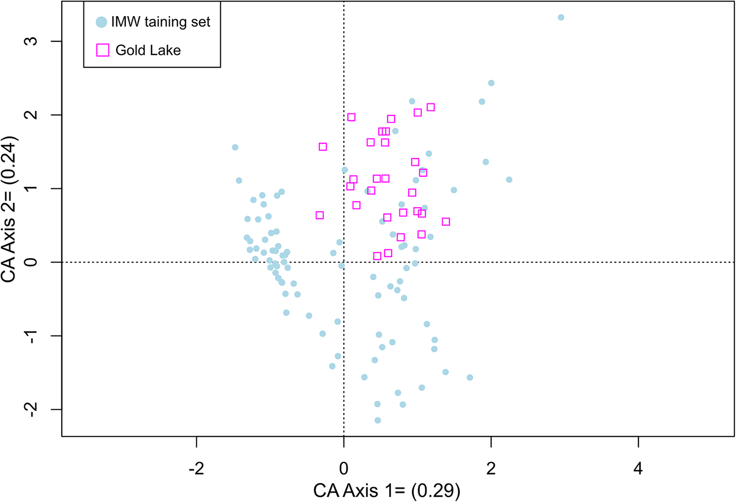
Correspondence analysis (CA) was used to plot sub-fossil chironomid assemblages from Gold Lake passively within an ordination of the IMW training-set lakes to determine the representation of the Gold Lake sub-fossil assemblages in the IMW training set. To maximize the signal-to-noise ratio (Prentice, Reference Prentice1980), relative abundance data were square-root transformed before ordination analyses. Correspondence analysis was performed using the vegan package in R (Oksanen, Reference Oksanen2008), while program C2 (Juggins, Reference Prentice2003) was used to develop the weighted averaging-partial least squares (WA-PLS) inference models and to estimate sample-specific errors. Prior to building the WA-PLS model, we updated estimates of MJAT at each of the 91 lakes in the IMW data set. The previous inference model of this data set (Haskett and Porinchu, Reference Haskett and Porinchu2014) was based upon MJAT estimates obtained from the PRISM Climate Group, which is at 800-meter resolution (PRISM Climate Group, http://www.prism.oregonstate.edu). In the mountainous terrain surrounding the IMW sites, temperatures vary greatly with elevation, such that the grid-cell temperature estimate may differ greatly from that at any specific elevation. Therefore, we used lapse-rate-adjusted estimates of MJAT using ClimateWNA software (Wang et al., Reference Wang, Hamann, Spittlehouse and Carroll2016). This software uses the same PRISM climate grids with the coarse-resolution elevation data underlying the PRISM data to develop a local temperature lapse rate and, thus, elevation-specific estimates of MJAT. Prior to running ClimateWNA, we verified the published name, size, elevation, and coordinates of the IMW lakes with maps from the USGS and Google Earth. We obtained lapse-rate-corrected estimates of MJAT for 1981–2010. Locations could not be verified for four lakes in the IMW database; thus, the originally published temperatures were used.
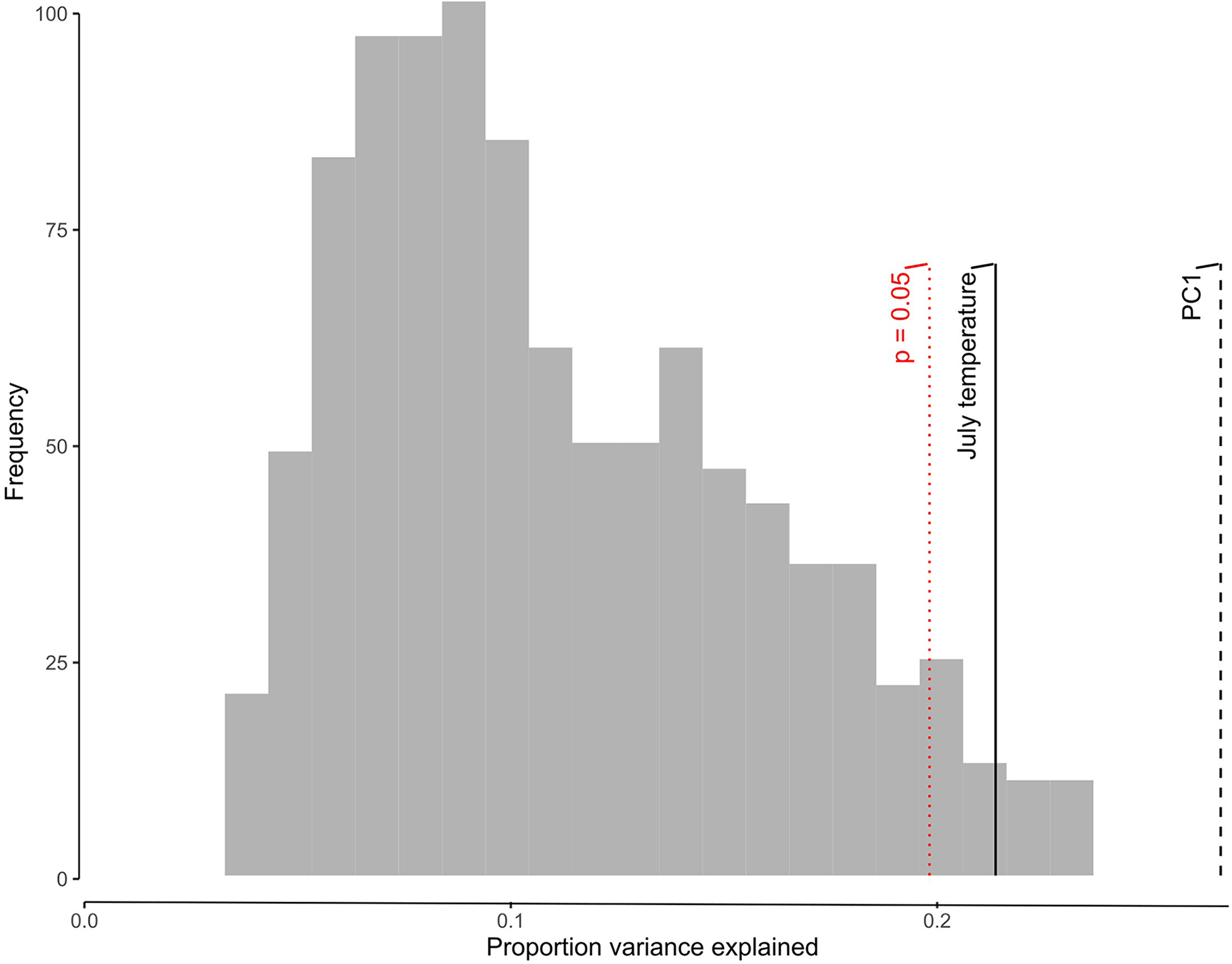
To assess the reliability of the chironomid-inferred MJAT reconstruction at Gold Lake, several criteria were considered. According to Heiri and Lotter (Reference Heiri and Lotter2001), a minimum of 50 head capsules should be present in each sample, and having > 95% of sub-fossil assemblages in the calibration dataset makes the quantitative environmental reconstruction highly reliable. Second, the proportion of rare taxa present in the down-core fossil samples was also used to evaluate the reliability of inference model estimates (Birks and Birks, Reference Birks and Birks1998). A taxon is classified as rare if the effective number of occurrences (or Hill’s N2) is ≤ 5 (Hill, Reference Hill1973). Reliable estimates of temperature optima can be obtained with taxa having Hill’s N2 values > 5 in the training set (Brooks and Birks, Reference Brooks and Birks2001). Third, we used the test of Telford and Birks (Reference Telford and Birks2011) to determine if the training set explains more variance of the fossil data set than explained if the environmental (temperature) data were randomized. A reconstruction is statistically significant if it explains more variance than the 95th percentile of reconstructions based on 999 transfer functions derived from transfer functions trained on random MJAT data.
Results
Chronology and sediment stratigraphy
Bayesian modeling in Bacon was used to develop an age-depth model (Blaauw and Christen, Reference Blaauw and Christen2011), where two radiocarbon ages were removed from the age-depth model because of a large measurement error or occurring out of stratigraphic order with the Mazama tephra age. Eleven radiocarbon dates that occurred in stratigraphic order remained part of the age-depth model (Table S1). A constant sedimentation rate was recorded from the base (1302 cm) up to 960 cm (0.071–0.11 cm/yr) from a 13-meter core that goes back to 14,500 years. There is a transition from silt and clay to sapropelic sediment at 50 cm above the core base (ca. 13.9 ka). Manually counted laminations were verified by three radiocarbon dates between 732–570 cm, confirming them as annual layers in the lake sediments (612 varves: 732–570 cm post-Mazama; 65 varves: 831–810 cm post-Llao to pre-Mazama). In the post-Mazama section up to 570 cm, the sedimentation rate is 6–7 times higher than the remainder of the core, after which it decreases and remains low through the Late Holocene (0.06–0.10 cm/yr) (Fig. 2; Baig and Gavin, Reference Baig and Gavin2023).
Sediment stratigraphy (left), percent loss-on-ignition (LOI, blue line), and Bacon age-depth model for Gold Lake (median estimates and 95% range shown by red and gray lines, respectively. Horizontal gray lines represent three tephra layers. Calibrated radiocarbon ages and uncertainty shown by horizontal blue lines. Age estimates in the varved section above the Mazama tephra are shown in light green at 10-cm intervals..

Except for the three tephra layers and a 50-cm segment at the bottom of the core (1302–1252 cm), the core is primarily composed of medium- to dark-brown biogenic sapropel. The core features sapropelic (biogenic) laminations (732–504 cm after the Mazama tephra and 20 cm from the Llao Rock tephra to the Mazama tephra), which are rhythmically banded in light and dark brown (830–810 cm). Silt and clay comprised the base sediment, with a relatively low loss-on-ignition (LOI) of 2–10%. The LOI values were 2–29% during the late-glacial period, 9–32% during the Early Holocene, and 15–34% during the Late Holocene. Around three of the detected tephra layers, LOI remained ∼5%, while laminated sections that formed after the Mazama eruption have lower LOI (10–15%) (Baig and Gavin, Reference Baig and Gavin2023).
Gold Lake chironomid diversity and community change
Thirty-one chironomid taxa were identified in 28 samples spanning the last 14,400 years. Taxon richness varies throughout the core, ranging between 8 and 16 extant taxa, with the highest richness occurring at ca.10 ka. Chironomus (14%), Corynocera near C. ambigua (19%), Corynocera oliveri type (7%), and Glyptotendipes (5%) were the most abundant taxa found (Fig. 3).
Relative abundance of chironomid taxa and taxon richness at Gold Lake. Taxa are arranged according to their MJAT optima inferred from the chironomid inference model with decreasing optima from left to right.

Gold-I: late-glacial period (1302–1110 cm; ca. 14.4–11.7 ka)
The chironomid community present in the postglacial period is dominated by Chironomus (11–40%), Glyptotendipes (0–32%), Microtendipes (0–25%), Corynocera near C. ambigua (2–19%), Einfeldia (14%), and Tanytarsini (5–14%) followed by Corynocera oliveri type (0–14%), Dicrotendipes (0–9%), Cricotopus/Orthocladius (4–8%). Cryptochironomus (4–7%), Synorthocladius (4–6%), and Procladius (2–8%), which appeared only in two samples, while Psectrocladius (11%) and Heterotrissocladius (4%) appeared only in one sample. Taxon richness varies between 8 and 14, with minimum richness at the bottom and highest at the top of the zone. Chironomus reaches its highest value in the core, ∼39%, at the bottom of the core, which eventually decreases to 10% at the zone top, while Microtendipes (24%) reach their highest core maximum at the zone top. Other taxa that also reach the highest percentages in the core are Cladotanytarsus (6%), Einfeldia (14%), Endochironomus (14%), Glyptotendipes (32%), and Synorthocladius (6%).
Gold II: Early/Middle Holocene–Pre-Mazama (1060–810cm; ca. 11.7–7.6 ka)
This zone is characterized by a diverse chironomid assemblage with taxon richness values between 10 and 17. The relative abundance of Corynocera near C. ambigua remains high, increasing up to 24% (6–24%) at the top of this zone, followed by Chironomus, which increases from 4% to 16% through the zone. Other taxa dominating this zone are Tanytarsus undifferentiated (4–14%) and Corynocera oliveri type (4–14%). Glyptotendipes (4–10%), and Microtendipes (2–10%) decrease in relative abundance compared to the previous zone. Other taxa that are present in minor percentages are Endochironomus, Cricotopus/Orthocladius, Cladotanytarsus, Heterotrissocladius, Microspectra, Procladius, and Psectrocladius.
The taxa Cladopelma, Polypedilum, Pagastiella, Paratendipes, Pentaneurini, Tanytarsus type-D, Chironomini-1st instar, Parakiefferiella, and Eukiefferiella appear for the first time. Some of the taxa that reached their highest values in this zone include Dicrotendipes, increases up to 25%, Cladopelma (6%), and Parakiefferiella (6%), while Pagastiella (4%) and Polypedilum (14%) appear only in this zone (Fig. 3).
Gold III: Middle Holocene–post-Mazama (732–-450 cm; ca. 7.6–4.25 ka)
Taxon richness in this zone ranges between 10 and 16. This zone is still dominated by Corynocera near C. ambigua, which reaches its core maximum of 33% at ca. 7.1 ka, followed by Chironomus, which increases up to 23% at ca. 5.5 ka after being low in abundance in the pre-Mazama zone. Other major taxa include Procladius and Tanytarsini (indeterminate), followed by Dicrotendipes (0–12%), Microtendipes (0–6%), Psectrocladius (0–4%), and Rheocricotopus (0–6%). This zone has a sample following the Mazama eruption, where 1.25 ml of sediment yielded only 37 head capsules.
Some of the other taxa that reach a core maximum include Corynocera oliveri-type (15%), Cricotopus/Orthocladius (14%), Chironomi-1st instar (10%), and Procladius (14%). Other taxa such as Parametriocnemus (6%), Eukiefferiella (6%), and Paratendipes (9%) reached a core maximum and did not appear in the remainder of the core. A number of other taxa did not appear after the Mazama eruption for ca. 300 cal yr, including Dicrotendipes, Einfeldia, Heterotrissocladius, and Pentaneurini, while Cladotanytarsus reappeared at ca. 5.5 ka. Some taxa appear for the first time, including Limnophyes, Sergentia, and Tanytarsus type-K (Fig. 3).
Gold IV: Late Holocene (350–0 cm; ca. 4.25 ka to present)
The chironomid community in this zone is dominated by Corynocera near C. ambigua (18–31%), Corynocera oliveri type (8–12%), followed by Chironomus, which fluctuates between 0% and 8% and reaches 31% at ca. 3.1 ka. The relative abundances of Tanytarsus type-D (2–4%) and Tanytarsus indeterminate (6–14%) increase during this interval.
Other taxa dominating the Late Holocene include Psectrocladius (0–16%), Rheocricotopus (0–12%), Sergentia (0–6%), Microspectra (0–10%), and Pentaneurini (0–6%), which reaches a core maximum in this zone. Limnophyes appears at ca. 0.9 ka with a maximum abundance of 8%. Taxa such as Dicrotendipes (2–8%) remain low in this zone, while Cricotopus/Orthocladius (4–12%) are not present after ∼ca. 1.9 ka. Einfeldia was absent in the remainder of the core after ca. 3.9 ka; Heterotrissocladius reappeared at ca. 2.5 ka with a higher relative abundance than the previous zone. Some taxa that reappeared in one or two samples with a low abundance include Cladopelma (2% at ca. 2.5 ka), Glyptotendipes (2–4%; ca. 2.5 ka and surface sample), Parakiefferiella (4% at ca. 2.4 ka and 1.4 ka), Synorthocladius (4% at ca. 1.4 ka), and Tanytarsus type-K (4% at ca. 3.1 ka). Taxon richness increased compared to the previous zone and varied between 11 and 15. The surface sample is dominated by Corynocera near C. ambigua, Corynocera oliveri type, Psectrocladius, and Rheocricotopus (Fig. 3).
Inference model using lapse-rate-adjusted MJAT
The (lapse-rate-adjusted) MJAT estimates for 91 lakes in the IMW data set varied substantially from the prior grid-cell estimates (Haskett and Porinchu, Reference Haskett and Porinchu2014). The difference in MJAT was large (> 1.0°C) for 18% of the lakes and > 0.25°C for 70% of the lakes. When comparing the two estimates across all training-set sites, there was a mean and maximum absolute deviation of 0.8°C and 5.7°C, respectively, and a root-mean-square error of 1.3°C.
The adjusted MJAT estimates for the IMW data set improved the performance of the inference models. Using a two-component weighted averaging-partial least squares (WA-PLS), including all taxa, resulted in a r2jack (a coefficient of determination) of 0.71, root mean square error of prediction (RMSEP) of 1.09°C, and maximum bias of 0.85°C (Table S3). In contrast, the prior model of Haskett and Porinchu (Reference Haskett and Porinchu2014) resulted in a r2jack of 0.61, RMSEP of 0.97°C, and a maximum bias of 2.22°C. Excluding rare taxa in our model (i.e., taxa present in < 5% of training-set lakes) during development of the inference model resulted in r2jack = 0.67, RMSEP = 1.09°C, and a maximum bias of 0.89°C. We chose to use the inference model with all taxa included to reconstruct Gold Lake temperature due to its higher r2jack and low maximum bias (Fig. 4).
Relationship between mean July air temperature derived using PRISM for the IMW calibration dataset and the midge-inferred mean July air temperature estimated using leave-one-out cross-validation. The solid line represents a 1:1 relationship.

Gold Lake chironomid-based MJAT
The Gold Lake chironomid assemblages and the IMW training-set assemblages were similar. Thirty-two chironomid taxa were identified in Gold Lake. Only four taxa (3% of identified head capsules) were not present in the IMW training-set lakes, including Chironomini-1stinstar (2.2%), Cryptochironomus (0.35%), Paratendipes (0.5%), and Parametriocnemus (0.21%). In addition, the assemblages of Gold Lake, plotted passively against the IMW training set using CA (Axis 1, λ = 0.29; Axis 2, λ = 0.24), show that the Gold Lake non-biting midges are located within the ordination space captured by the IMW training set (Fig. 5). The sample-specific error estimates associated with Gold Lake MJAT estimates vary between 1.0°C and 2.0°C. The taxa present in Gold Lake are well represented in the IMW calibration set with Hill’s N2 diversity index (Hill, Reference Hill1973) ranging between 9 and 57 for 22 taxa. Although six additional taxa have Hill’s N2 values below 4, the proportion of rare taxa is low as they are present in fewer than 7 samples and do not dominate the assemblages, except for Glyptotendipes and Einfeldia. The MJAT reconstruction also passed the significance test of Telford and Birks (Reference Telford and Birks2011) with a value of p = 0.025 (Fig. 6). Overall, the above tests indicate that the reconstruction can be considered to be reliable based on the representation of the Gold Lake non-biting midge taxa in the training set (Birks and Birks, Reference Birks and Birks1998).
Correspondence analysis (CA) passively plotting Gold Lake midge assemblages with chironomid assemblages of IMW; CA Axis 1: λ = 0.29; CA Axis 2: λ = 0.24.

The results of Telford and Birks (Reference Telford and Birks2011) significance test. The histogram depicts the fraction of variation explained in the fossil data by 999 transfer functions trained on random environmental data. The solid line represents the proportion of variation explained by reconstructed MJAT in the fossil record using the MJAT inference model. The dotted line ‘PC1ʹ represents the highest proportion of variance explainable (i.e., axis 1 of the CA of the fossil samples). The Gold Lake reconstruction is statistically significant because it explains more of the variance in the fossil data than 95% of the reconstructions derived from transfer functions trained on random environmental data (red line).

Temperature reconstruction
The average midge-inferred MJAT for Gold Lake for the last 14.5 ka is 11.3°C (Fig. 7E). During the late-glacial period (14.4–11.6 ka), the MJAT remained low (9.3–10.8°C), or 0.5–2.0°C below the long-term average. The lowest temperature (9.0°C) occurred within the Younger Dryas at ca. 12.7 ka.
(A, B) January insolation and July insolation values, respectively, in watts/m2 at 40°N. (C) δ18O at Oregon Caves (Ersek et al., Reference Ersek, Clark, Mix, Cheng and Edwards2012). (D) Northeast Pacific sea-surface temperature (SST) inferred from alkenone records from cores near northern California (Barron et al., Reference Barron, Heusser, Herbert and Lyle2003). (E) Chironomid-based mean July air temperature (MJAT: black line with blue dots) reconstruction for Gold Lake; horizontal dashed black line represents the mean reconstructed MJAT.

The Holocene–pre-Mazama period (11.6–7.6 ka; 10.9–12.0°C) is marked by a sudden increase in temperature of 0.8°C (10.2–11.0°C) that reaches 12.0°C at 9.2 ka and remains high until 8 ka when it decreased to 10.9°C immediately before the Mazama eruption. The transition into the Middle Holocene post-Mazama (7.6–5 ka;10.8–12.6°C) is marked by a sudden increase in midge-inferred MJAT (10.9–12.0°C). MJAT remained high until 7.3 ka, after which time it dropped to 10.7°C at 7.1 ka and then increased to 11.1°C in the adjacent sample at ca. 6.8 ka. MJAT decreased towards the end of the Middle Holocene and reached 10.8°C at ca. 5.6 ka. During the Late Holocene, midge-inferred MJAT increased to the highest recorded temperature of ∼13.1°C at 2.5 ka and then decreased to 11.6°C at 1.9 ka. MJAT remained high during the last ca. 2 ka, fluctuating between 12.2°C and 12.6°C.
Discussion
Gold-I: late-glacial period (1302–1110 cm; ca. 14.4–11.7 ka)
The Gold Lake non-biting midge stratigraphy reveals large changes in the community structure and inferred temperature since deglaciation. The late-glacial period, especially ca. 14.4–13 ka, is dominated by Chironomus, Dicrotendipes, Glyptotendipes, Einfeldia, and Corynocera near C. ambigua—taxa that are found today in eutrophic to mesotrophic lakes (Brodersen et al., Reference Brodersen, Odgaard, Vestergaard and Anderson2001; Brooks et al., Reference Brooks, Langdon and Heiri2007). These taxa decreased during the Younger Dryas period and remained low during the transition into the Early Holocene with the exception of Microtendipes, which reached a core maximum at ca. 12 ka, and Corynocera near C. ambigua, which increased to 19%. Corynocera oliveri-type, commonly associated with cold water (Brooks et al., Reference Brooks, Langdon and Heiri2007), was present consistently, with its maximum abundance occurring in the bottom sample of the late-glacial period.
During the late-glacial period, the non-biting midge community is marked by early colonizing taxa, which are typical of hypoxia, low pH, and cold water. Chironomus, considered an early colonizer of lakes (Brooks et al., Reference Brooks, Mayle and Lowe1997) and commonly confined to the deeper parts of lakes in hypoxic to anoxic conditions (Brooks et al., Reference Brooks, Langdon and Heiri2007), was present in maximum abundance at the bottom sample of the late-glacial period. Glyptotendipes appears at ca. 13.8 ka, reaching a maximum abundance (32%) before decreasing to almost 20% for the rest of this zone. The appearance of Cladotanytarsus for the first time with its maximum abundance (6%) at 13.2 ka may reflect decreasing pH (Henrikson et al., Reference Henrikson, Olofsson and Oscarson1982). A higher abundance of Glyptotendipes during this time further supports the inference of low pH as it is an acidophilic taxon (Brodin, Reference Brodin1986). The occurrence of Dicrotendipes, Cladotanytarsus, and Einfeldia at ca. 13.4 ka suggests the potential establishment of aquatic macrophytes in the littoral zone (Brodersen et al., Reference Brodersen, Odgaard, Vestergaard and Anderson2001; Langdon et al., Reference Langdon, Ruiz, Brodersen and Foster2006). Cricotopus/Orthocladius was consistently present during the late-glacial period and is commonly associated with standing and flowing waters (Brooks et al., Reference Brooks, Langdon and Heiri2007) and aquatic vegetation (Brodin, Reference Brodin1986).
The Gold Lake midge-inferred temperature matches well with the Northern Hemisphere pattern of sudden warming at ca. 14.7 ka, followed by a cold reversal (Younger Dryas) at ca. 12.7 ka, which persisted until the start of the Holocene (Lotter Eawag et al., Reference Lotter Eawag, Eicher, Siegenthaler and Birks1992). The high percentages of Chironomus and Glyptotendipes contributed to the elevated midge-inferred MJAT of 10.9–9.8°C between 14.3–13.2 ka. The decline in MJAT to 9.4°C during the Younger Dryas period at ca. 12 ka was driven by the increase in Einfeldia, Synorthocladius, and Corynocera near C. ambigua and the presence of the cold-adapted taxon Corynocera oliveri type. The Gold Lake record suggests that the late-glacial period (10.6°C), ca.14.3 ka, was characterized by a MJAT that was 1.6°C lower than the inferred modern temperature. This pattern agrees with the inferred temperature at Lake Stowell and Windy Lake, British Columbia (Chase et al., Reference Chase, Bleskie, Walker, Gavin and Hu2008; Lemmen and Lacourse, Reference Lemmen and Lacourse2018).
During the Younger Dryas, Gold Lake MJAT reached its minimum at 9.4°C, which is 2.8°C lower than modern, and coincides with many other proxy-based temperatures showing a decline in temperature during Younger Dryas (Mathewes, Reference Mathewes1993; Barron et al., Reference Barron, Heusser, Herbert and Lyle2003; Lacourse, Reference Lacourse2005; MacDonald et al., Reference MacDonald, Moser, Bloom, Porinchu, Potito, Wolfe, Edwards, Petel, Orme and Orme2008). Gavin et al. (Reference Gavin, Brubaker and Greenwald2013) also suggested, based on the midge-inferred paleotemperature from southern British Columbia, that MJAT was 2.5°C lower than present during the Younger Dryas.
Gold II: Early/Middle Holocene–pre-Mazama (1060–810cm; ca. 11.7–7.6 ka)
During the Early/Middle Holocene, there was an increase in the abundance and diversity of warm-adapted taxa at Gold Lake. Dicrotendipes increased to 25%, and Polypedilum appeared for the first time, reaching its maximum abundance (14%). These taxa drive an increase in MJAT to 11°C from 10.2°C, reflecting an elevated temperature (Brodersen et al., Reference Brodersen, Odgaard, Vestergaard and Anderson2001). Increased abundance of Dicrotendipes in the Intermountain West region has been associated with increased temperature during the late twentieth century (Porinchu et al., Reference Porinchu, Potito, MacDonald and Bloom2007; Reinemann et al., Reference Reinemann, Porinchu and Mark2014b), and this taxon has been identified as a thermophilic taxon in the IMW dataset (Haskett and Porinchu, Reference Haskett and Porinchu2014). Paratendipes, Cladopelma, and Pagastiella appear for the first time at ca. 11.1 ka, followed by Polypedilum and Pentaneurini, with maximum abundance in the core at ca. 10.2 ka supporting the inference of increased temperature during this interval (Cranston et al., Reference Cranston, Oliver, Sæther and Wiederholm1983). The occurrence of Polypedilum, Paratendipes, and Psectrocladius at 10.2–8.6 ka may reflect the presence of aquatic macrophytes in the lake’s littoral zone, elevated temperature (Brodin, Reference Brodin1986), and possibly a lowering of the lake level (Cranston et al., Reference Cranston, Oliver, Sæther and Wiederholm1983). Taxa such as Pagastiella, Pentaneurini, and Polypedilum, have high MJAT optima in the Intermountain West training set (Haskett and Porinchu, Reference Haskett and Porinchu2014). The presence of these species suggests that Gold Lake was warmer and more productive during the Early Holocene. Gold Lake MJAT deviates between −0.3–1.3°C from the long-term average, compared to −1.9°C to −0.4°C for the late-glacial period. Notably, at 9.2 ka, the temperature reached 12.0°C and remained high until 8 ka with a MJAT of 10.9°C immediately prior to Mazama eruption ca. 7.63 ka. The elevated temperature at Gold Lake during this interval coincides with the maximum summer insolation in the Pacific Northwest with dry summers (Heusser et al., Reference Heusser, Heusser and Peteet1985; Bartlein et al., Reference Bartlein, Anderson, Anderson, Edwards, Mock, Thompson, Webb, Webb and Whitlock1998; Walker and Pellatt, Reference Walker and Pellatt2003); however, it did not exceed the modern recorded temperature.
Before the Mazama eruption, some thermophilous taxa decreased (e.g., Chironomus, Glyptotendipes, and Microtendipes). At the same time, cold-adapted taxa such as Corynocera near C. ambigua, Corynocera oliveri-type, and Heterotrissocladius increased (Walker and Mathewes, Reference Walker and Mathewes1988). Evidence of cooling prior to the Mazama eruption has also been inferred from a pollen–climate transfer function for Coastal British Columbia (Mathewes and Heusser, Reference Mathewes and Heusser1981). During this zone (8–7.63 ka), the MJAT remained low, approximately −0.1 to −0.4°C below the long-term average, while during 9.2–8.6 ka, it remained above the long-term average, approximately 0.4–0.7°C (Fig. 7).
Gold III: Middle Holocene–post-Mazama (732–350 cm; ca. 7.6–4.25 ka)
After the Mazama tephra deposition at ca. 7.6 ka, MJAT increases to 11.5°C and reaches a maximum of approximately 12.6°C at ca. 7.2 ka, 1.3°C above the long-term average for the last 14.5 ka. Following this interval of elevated temperature, MJAT decreases and remains low relative to the Early Holocene. This pattern agrees with evidence of Northern Hemisphere cooling during the Middle Holocene (Marcott et al., Reference Marcott, Shakun, Clark and Mix2013) and cooler summers along the North Pacific coast (Barron et al., Reference Barron, Heusser, Herbert and Lyle2003; Praetorius et al., Reference Praetorius, Mix, Walczak, Wolhowe, Addison and Prahl2015), likely driven by decreasing summer insolation (Berger and Loutre, Reference Berger and Loutre1991). Transition to lower temperatures at Gold Lake started at ca. 7 ka, while at Windy Lake and Thunder Lake, British Columbia, it occurred at 6 ka and 4.5 ka, respectively (Chase et al., Reference Chase, Bleskie, Walker, Gavin and Hu2008).
During the Early Holocene at Gold Lake, peak warmth occurred at 7.2 ka shortly following the tephra deposition. An increase in Pentaneurini and Tanytarsus type-D, which have MJAT optima of 12.4°C and 14.6°C, respectively, coincide with increased temperature reconstructed at Gold Lake (Haskett and Porinchu, Reference Haskett and Porinchu2014). This inferred warming may partly be caused by the ‘aridification’ effect of the tephra, reducing the leaf area of the surrounding vegetation and reducing latent heat flux, thus increasing the sensible heat (Harris and Van Couvering, Reference Harris and Van Couvering1995). Peak warmth at sites farther to the south occurred later in the Holocene: at Stella Lake, Great Basin, the temperature peaked at 5.4 ka at 11.0°C (Reinemann et al., Reference Reinemann, Porinchu, Bloom, Mark and Box2009), while at Pyramid Lake, Nevada, a δ18O record shows the warmest interval during the Holocene was at ca. 6.8 ka (Benson et al., Reference Benson, Kashgarian, Rye, Lund, Paillet, Smoot, Kester, Mensing, Meko and Lindström2002). A site in eastern Nevada provides evidence for peak Holocene warmth at 6.5 ka (Potito et al., Reference Potito, Porinchu, MacDonald and Moser2006), while at a site to the north (in southern British Columbia), peak warmth occurred earlier in the Holocene, closer to 9 ka (Chase et al., Reference Chase, Bleskie, Walker, Gavin and Hu2008). Following the short-lived period of post-Mazama warmth, cold-adapted and thermophilous taxa varied in relative abundance, resulting in fluctuating MJAT.
Gold IV: Late Holocene (350–0 cm; ca. 4.25 ka to present)
During the Late Holocene, midge-inferred MJAT reaches a maximum of 13.7°C at 2.5 ka, after which time it decreases to 11.7°C at 1.9 ka and then fluctuates between 12.2°C and 12.6°C for the remainder of the record. MJAT inferred temperature increases from 10.8°C to 11.4°C at the bottom of this zone, which is 0.09°C above the long-term average, and remained high for the rest of the core, fluctuating between 0.04°C and 1.8°C, except at 3.1 ka, where it was 0.3°C below the long-term average MJAT.
During the Late Holocene, taxa associated with warmer, more productive conditions (e.g., Dicrotendipes, Microtendipes, and Tanytarsus type-D) increased (Brodersen et al., Reference Brodersen, Odgaard, Vestergaard and Anderson2001; Brooks et al., Reference Brooks, Langdon and Heiri2007; Porinchu et al., Reference Porinchu, Potito, MacDonald and Bloom2007) and taxa associated with cooler, less productive conditions (e.g., Chironomus and Corynocera near C. ambigua) decreased. At 2.5 ka, when MJAT reaches its maximum (13.7°C), a taxon associated with eutrophic lakes, Cladopelma, appears for the first time (Cranston et al., Reference Cranston, Oliver, Sæther and Wiederholm1983) along with Parakiefferiella bathophila-type, Dicrotendipes, Microtendipes, and Procladius (Wiederholm, Reference Wiederholm1983; Walker et al., Reference Walker, Smol, Engstrom and Birks1991; Brooks et al., Reference Brooks, Langdon and Heiri2007; Haskett and Porinchu, Reference Haskett and Porinchu2014)). Between 4.5 and 3.5 ka, ENSO activities were intensified, resulting in Indo-Pacific warming (Donders et al., Reference Donders, Wagner-Cremer and Visscher2008). Proxy data from Castor Lake in Washington also suggests a basin-scale change during 4–5 ka in the Pacific Ocean with variability in drought conditions (Nelson et al., Reference Nelson, Abbott, Steinman, Polissar, Stansell, Ortiz, Rosenmeier, Finney and Riedel2011).
During the Medieval Climate Anomaly (MCA), MJAT at Gold Lake is 1.2°C above the long-term average for the last 14.5 ka. The warming episode recorded at Gold Lake preceded the MCA, starting at 1.4 ka when MJAT was 1.28°C above the long-term average. A similar pattern was recorded at Stella Lake, where MJAT was 0.4°C above the Late Holocene average during the MCA (Reinemann et al., Reference Reinemann, Porinchu, MacDonald, Mark and DeGrand2014a). During the Little Ice Age (LIA), MJAT at Gold Lake was 0.09°C below the mean MCA temperature but was 1.10°C above the long-term average. At Stella Lake, MJAT was ∼1.0°C below the 2000-year mean temperature (Reinemann et al., Reference Reinemann, Porinchu, MacDonald, Mark and DeGrand2014a), with MJAT 1.5°C below peak Holocene warmth (Reinemann et al., Reference Reinemann, Porinchu, Bloom, Mark and Box2009). After the LIA, the temperature declined, reaching 12.3°C in the uppermost sediment. This temperature is slightly below the MJAT inferred during the MCA. Maximum temperature (13.2°C) during Late Holocene at ca. 2.5 ka at Gold Lake agrees with the Northeast Pacific sea-surface temperature (SST) that recorded a permanent increase up to 1.0°C in alkenone SST at ca. 3.2 ka, which reflects an increasing wintertime insolation in northern California (Barron et al., Reference Barron, Heusser, Herbert and Lyle2003). The chironomid record from Lake Stowell, a low-elevation lake, also shows a Late Holocene increase in July air temperature at about the same time (ca. 2 ka) (Lemmen and Lacourse, Reference Lemmen and Lacourse2018). There might be a general link between SST and high-elevation temperature, possibly by affecting the lapse rate. Increased Late Holocene precipitation, widely documented in the Pacific Northwest, could have resulted in more latent heat transfer and decreased lapse rates, contributing to the reconstructed increase in Late Holocene temperature at Gold Lake.
Timing of the increased temperature at Gold Lake corresponds well to warming events in the Northern Hemisphere reconstructed based on pollen (PAGES 2k Consortium, 2013), midge-inferred reconstruction at Stella Lake, Central Great Basin, Nevada (Reinemann et al., Reference Reinemann, Porinchu, MacDonald, Mark and DeGrand2014a), and other reconstructions done in the Northern Hemisphere (Moberg et al., Reference Moberg, Sonechkin, Holmgren, Datsenko, Karlén and Lauritzen2005; Mann et al., Reference Mann, Zhang, Rutherford, Bradley, Hughes, Shindell, Ammann, Faluvegi and Ni2009). At Gold Lake, we observed the recorded high temperature at ca. 2.5 ka, but it seems, based on the above-recorded data, it might have started earlier. Chironomid-based MJAT reconstructions at higher, decadal-scale resolution could potentially fill the present gap in available data and confirm this hypothesis.
Conclusion
This is the first study of chironomids and paleotemperature reconstruction in the Pacific Northwest from the late-glacial period to the present. Quantitative reconstructions based on chironomids are still rare and are still developing in the USA. Gold Lake midge-inferred MJAT suggests a cool late-glacial period with ∼10.6°C, which is 1.6°C cooler than the modern temperature. The Younger Dryas event was clearly recorded with a minimum temperature of 9.4°C followed by an increasing trend of temperature in transition into the Early Holocene. The temperature increased during the Early Holocene to ∼12.0°C at 9.2 ka with increased abundance of the thermophilous taxa.
The Middle Holocene was cooler overall than the Early Holocene. The highest temperature was recorded during the Late Holocene at ca. 2.5 ka, which generally coincides with the Northeast Pacific sea-surface temperature, which recorded a permanent increase up to 1.0°C in alkenone SST at ca. 3.2 ka (Barron et al., Reference Barron, Heusser, Herbert and Lyle2003).
Overall, the Late Holocene appears to be the warmest portion of the Holocene period and has clear evidence of increased temperature during the MCA, although sample resolution was insufficient to resolve the MCA and LIA in detail. This chironomid MJAT record, although coarsely sampled (multi-centennial intervals), produced new findings of the effect of Mazama tephra on local temperatures, potentially due to an aridification effect of the deep tephra deposit. This suggests that further studies, including multiple lakes from the Pacific Northwest and increased temporal resolution, are crucial to placing the projected climatic changes into a long-term context. In addition, while the IMW training data set was well suited for reconstructing temperatures from the Gold Lake record, expanding this calibration data set to a broader suite of lakes in the Pacific Northwest will increase its applicability for temperature reconstruction from lakes in the Pacific Northwest.
Acknowledgments
JB and DGG conceptualized the study, devised the methodology, and conducted the field investigation. JB acquired the funding and curated, analyzed, and visualized the data. IW and DP helped in chironomid identification and classification. JB wrote the original manuscript, and DGG reviewed, edited, and contributed to the final manuscript. IW and DP contributed to editing and finalizing the manuscript. Gold Lake data are available on the Neotoma Paleoecology Database, and the IMW calibration dataset is available at https://hdl.handle.net/1794/30185.
This research work was funded by the University of Oregon Lokey Doctoral Science Fellowship, Oregon Lakes Association Scholarship, and grants from the University of Oregon Departments of Environmental Studies (Soderwall Foundation Research Support) and Geography (Rippey Dissertation Grant). The authors declare that they have no known competing financial interests or personal relationships that could have appeared to influence the work reported in this paper.
The authors would like to thank Chantel Saban, Lauren Hendricks, and Briana Kendrick for their help during fieldwork. We also thank detailed feedback from Derek Booth (Senior Editor), Terri Lacourse (Associate Editor), and two anonymous reviewers that greatly improved the manuscript.
Jamila Baig’s current affiliation is Department of Biology, Washington and Lee University, Lexington, VA.