



1. Introduction
The multitype branching process (MBP) on an at most countable set X is a process which describes the evolution of a population breeding and dying on X, where the elements of X can be seen as types or positions of the individuals of the population. Throughout our paper we stick with the second interpretation and we consider X as the space where the dynamics take place. Another common name for this process is a branching random walk, although some authors reserve this denomination for the case when X is endowed with a graph structure (and the types/locations of the children are chosen independently according to a transition matrix). Multitype branching processes have been a research subject since the beginning of the focus on branching mechanisms (see [Reference Harris14]) and have been studied over the years by several authors ([Reference Biggins, Cohn and Nerman10, Reference Gantert, Müller, Yu and Vachkovskaia13, Reference Jagers and Nerman16, Reference Machado, Menshikov and Popov19, Reference Menshikov and Volkov22] to mention a few).
A general MBP is defined once we fix the reproduction law
 ${\boldsymbol{\mu}}=\{\mu_x\}_{x\in X}$
(see Section 2.1 for details). All particles at site x reproduce and place children according to
 $\mu_x$
, which incorporates not only information about how many children there are, but also about where they are sent to live. In this sense particles do not walk, but there is a random walk of the population as a whole.
The branching process can be seen as a particular case of the MBP, where X is reduced to a singleton and the only information needed is the reproduction law
 $\rho$
defined on
 $\mathbb{N}$
. A natural way to define an MBP on X is to couple a family of branching processes, given by reproduction laws
 $\{\rho_x\}_{x\in X}$
, and a random walk with transition matrix P on X. Each individual at x has a
 $\rho_x$
-distributed number of offspring, which are independently dispersed according to the random walk. We call this kind of process an MBP with independent diffusion. We remark that for general MBPs, the dispersal of the progeny may not be independent nor based on a random walk (for instance we may place two children at a given vertex with probability p and one child at each of a couple of other vertices with probability
 $1-p$
).
We are interested in the long-term behaviour of the process in fixed subsets of X. In the long run, for any
 $A\subseteq X$
, an MBP starting with one individual at
 $x\in X$
can go extinct in A (no individuals alive in A from a certain time on) or survive in A (infinitely many visits to A). If the probability of extinction in A is equal to 1, we say that there is extinction in A, and we say that there is survival in A otherwise. There is global survival when there is survival in X, and we have strong survival in A when, conditioned on global survival, there is survival in A almost surely. There is local survival in x when
 $A=\{x\}$
.
Clearly, the probability of extinction in A depends on the starting vertex x. Then, letting x vary in X, we get an extinction probability vector that we denote by
 $\mathbf{q}(A)$
. If we allow A to vary among the subsets of X, we have the family of all extinction probability vectors of the MBP.
For the branching process, it is well known that long-term behaviour and the extinction probability are related to the generating function of
 $\rho$
,
 $G(z)\,:\!=\,\sum_n\rho(n)z^n$
,
 $z\in[0,1]$
. Provided that the process is nontrivial, i.e.
 $\rho(1)<1$
, this generating function has at most two fixed points: the extinction probability and 1. In the case of a general MBP it is possible to define a (multidimensional) generating function which plays a similar role, but as soon as X is not finite, the situation gets far more complex: there might be infinitely many fixed points and infinitely many extinction probability vectors (see Section 2.3); moreover, there can be fixed points that are not extinction probability vectors. It is still true, however, that the vector
 $\mathbf{1}$
is always a fixed point of the generating function and the global extinction probability vector (i.e. the probability of extinction in the whole space X) is always the smallest fixed point.
The fact that the generating function of the process contains all the information on its behaviour is exploited in the main result of the present paper. In [Reference Hutchcroft15] the author focused on MBPs with independent diffusion and equal reproduction law
 $\rho$
at all sites and introduced a new stochastic ordering. This order is named germ order and is based on a comparison between the one-dimensional generating functions of the reproduction laws. The author was able to compare MBPs that are defined by the same underlying random walk P on X and differ only by the reproduction law, which is constant along X.
We define the germ order for general MBPs, which extends the one in [Reference Hutchcroft15], thus comparing multidimensional generating functions. The fact that our definition is indeed a generalisation is proved in Proposition 2.3 (see also the discussion preceding the proposition itself). We extend [Reference Hutchcroft15, Theorem 1.3] by proving the following result (a more precise statement is given by Theorem 4.1).
Theorem 1.1. Let
 ${\boldsymbol{\mu}}$
and
 ${\boldsymbol{\nu}}$
be the laws of two MBPs on a countable space X, and let
 $\boldsymbol{\mu} \mathbin{\ge_{\mathrm{germ}}} \boldsymbol{\nu}$
.
-
(i) In any set where there is
 ${\boldsymbol{\nu}}$
-survival, there is
${\boldsymbol{\mu}}$
-survival.
-
(ii) If the supremum of the global
${\boldsymbol{\nu}}$
-extinction probabilities, over all starting coordinates, is smaller than 1, then in any set where there is
${\boldsymbol{\nu}}$
-strong survival, there is
${\boldsymbol{\mu}}$
-strong survival.


The assumption in the second part of the statement may appear technical at first glance, but as discussed in Section 4, it cannot be removed. Moreover, it is worth remarking that under very mild conditions, among all fixed points, only the global extinction probability vector may have a strictly smaller than 1 upper bound for the supremum of its components. Indeed, we extend a result of [Reference Moyal23], which stated that, under certain conditions, the global extinction probability vector is the only fixed point that may have coordinates bounded from above by some
 $\delta<1$
. We are able to prove, in Theorem 3.1, that under no conditions at all, the global extinction probability vector is the only extinction probability vector that can have this property. Moreover, if a mild condition is satisfied, it is also the only fixed point with supremum different from 1. This result allows us to overcome the issues which arise in the multidimensional case and to extend [Reference Hutchcroft15, Theorem 1.3] to general MBPs.
The paper is organised as follows. Section 2 is devoted to the basic definitions and preliminary results. In Section 3 we deal with extinction probabilities and prove Theorem 3.1 Section 4 is devoted to the relation between survival (resp. strong survival) for two MBPs satisfying the germ order. The main result of the section, Theorem 4.1, deals with the germ order and with probability-generating function order as a particular case. The proofs of the technical lemmas can be found in the Appendix.
2. Basic definitions and preliminaries
2.1. Generating functions, MBPs, and ordering
Given an at most countable set X and a set Y, we consider a family of measures
 ${\boldsymbol{\mu}}=\{\mu_y\}_{y \in Y}$
defined on the (countable) measurable space
 $S_X\,:\!=\,\{f\colon X \to \mathbb{N}\colon |f|<+\infty\}$
equipped with the
 $\sigma$
-algebra
 $2^{S_X}$
where
 $|f|\,:\!=\,\sum_{x\in X}f(x)<+\infty$
; throughout this paper we denote by
 $\mathbb{N}$
the set of natural numbers including 0. An interpretation is the following. Suppose that an individual marked with a label y has a random number of items to place in a space X; then
 $\mu_y(f)$
represents the probability that there are f(x) items placed at x (for all
 $x \in X$
).
With the family
 $\{\mu_y\}_{y \in Y}$
, we associate the following generating function
 $G_{\boldsymbol{\mu}}\colon[0,1]^X \to [0,1]^Y$
:
 \begin{equation} G_{\boldsymbol{\mu}}({\mathbf{z}}|y) \, :\!= \, \sum_{f \in S_X} \mu_y(f) \prod_{x \in X} {\mathbf{z}}(x)^{f(x)},\end{equation}
where
 $G_{\boldsymbol{\mu}}({\mathbf{z}}|y)$
is the y coordinate of
 $G_{\boldsymbol{\mu}}({\mathbf{z}})$
. The family
 $\{\mu_y\}_{y \in Y}$
is uniquely determined by
 $G_{\boldsymbol{\mu}}$
(see, for instance, [Reference Bertacchi and Zucca6, Section 2.3] or [Reference Bertacchi and Zucca7, Section 2.2], and Lemma 2.1. Let
 $\mathbf{0}, \mathbf{1} \in [0,1]^X$
be such that
 $\mathbf{1}(x)\,:\!=\,1$
and
 $\mathbf{0}(x)\,:\!=\,0$
for all
 $x \in X$
. We define
 $\phi^{\boldsymbol{\mu}}_y(t)\,:\!=\,G_{\boldsymbol{\mu}}(t\mathbf{1}|y)$
for
 $t \in [0,1]$
and
 $y \in Y$
. Note that, if
 $\rho_y(n)\,:\!=\, \mu_y(\, f\colon |f|=n)$
, then
 $\phi_y$
is the one-dimensional generating function of
 $\rho_y$
. Henceforth, when it is not misleading, we drop the sub/superscripts and write G and
 $\phi$
. The topological properties of G are described in the following proposition, whose proof is left to the reader. In particular, we denote by
 $\|\mathbf{z}\|_\infty\,:\!=\,\sup_{x \in C} |\mathbf{z}(x)|$
the restriction of the norm of
 $l^\infty(C)$
to
 $[0,1]^C$
(for
 $C\in\{X,Y\}$
).
Proposition 2.1. Let us consider the generating function G defined by (2.1).
-
(i) G is non-decreasing with respect to the usual partial order of
$[0,1]^X$
and
$[0,1]^Y$
. -
(ii) G is continuous with respect to the pointwise convergence topology of
$[0,1]^X$
and
$[0,1]^Y$
. -
(iii) If the family
$\{\rho_y\}_{y \in Y}$
is tight then G is uniformly continuous with respect to the
$\|\cdot\|_\infty$
topologies of
$[0,1]^X$
and
$[0,1]^Y$
.


A particular family of measures
 ${\boldsymbol{\mu}}$
is the multinomial one, which is defined given a family
 $(\rho_y)_{y \in Y}$
of measures on
 $\mathbb{N}$
and a nonnegative stochastic matrix
 $P=(p(y,x))_{y \in Y, x \in X}$
(where
 $\sum_{x \in X} p(y,x)=1$
for all
 $y \in Y$
). We say that
 ${\boldsymbol{\mu}}$
is a multinomial family of measures if
 \begin{equation} \mu_y(f) = \rho_y\Bigg(\sum_{x\in X}f(x)\Bigg)\frac{\big(\sum_{x\in X}f(x)\big)!}{\prod_{x\in X}f(x)!} \prod_{x \in X} p(y,x)^{f(x)} \quad \text{for all}\ f \in S_X.\end{equation}
We can interpret multinomial families as measures where individuals marked with the label y draw a random number n of items (according to
 $\rho_y$
) and place each of them independently in X according to the distribution
 $\{p(y, \cdot)\}$
. It is easy to prove that for a multinomial family
 ${\boldsymbol{\mu}}$
,
 \begin{equation} G(\mathbf{z}|y)=\phi^{\boldsymbol{\mu}}_y (P\mathbf{z}(y)) \quad \text{for all}\ y \in Y, \, \mathbf{z} \in [0,1]^X,\end{equation}
where
 $P\mathbf{z}(y)=\sum_{x \in X} p(y,x)\mathbf{z}(x)$
. In fact, using the definitions of G and
 $\phi^{\boldsymbol{\mu}}$
, and (2.2),
 $G(\mathbf{z}|y)$
can be written as
 \[ \sum_{n\in\mathbb{N}}\rho_y(n)\sum_{|f|=n}\frac{n!}{\prod_{x\in X}f(x)!}\prod_{x\in X}(p(y,x)\mathbf{z}(x))^{f(x)} = \sum_{n\in\mathbb{N}}\rho_y(n)\Bigg(\sum_{x\in X}p(y,x)\mathbf{z}(x)\Bigg)^n.\]
When
 $Y=X$
, the family
 ${\boldsymbol{\mu}}$
and its generating function
 $G_{\boldsymbol{\mu}}$
identify a discrete-time MBP on X, which we denote by
 $(X,{\boldsymbol{\mu}})$
. This is a process
 $\{\eta_n\}_{n \in \mathbb{N}}$
, where
 $\eta_n(x)$
is the number of particles alive at
 $x \in X$
at time n. The dynamics is as follows. A particle of generation n, at site
 $x\in X$
, lives one unit of time; after that, a function
 $f \in S_X$
is chosen at random according to the law
 $\mu_x$
. This function describes the number of children and their positions. The choice of f is independent for all breeding particles.
An explicit construction is the following. Given a family
 $\{ f_{i,n,x}\}_{i,n \in \mathbb{N}, x \in X}$
of independent
 $S_X$
-valued random variables such that, for every
 $x \in X$
,
 $\{f_{i,n,x}\}_{i,n \in \mathbb{N}}$
have the common law
 $\mu_x$
, then the discrete-time MBP
 $\{\eta_n\}_{n \in \mathbb{N}}$
is defined iteratively as
 \begin{equation} \eta_{n+1}(x) = \sum_{y\in X}\sum_{i=1}^{\eta_n(y)}f_{i,n,y}(x) = \sum_{y \in X} \sum_{j=0}^\infty 1_{\{\eta_n(y)=j\}} \sum_{i=1}^{j} f_{i,n,y}(x)\end{equation}
starting from an initial condition
 $\eta_0$
. The actual canonical construction of
 $\{\eta_n\}_{n \in \mathbb{N}}$
can be carried on, by using Kolmogorov’s theorem, in such a way that the probability space and the process
 $\{\eta_n\}_{n \in \mathbb{N}}$
are fixed, while the probability measure depends on the starting configuration and the family
 ${\boldsymbol{\mu}}$
.
When the initial configuration is
 $\eta\in\mathbb{N}^X$
, the corresponding law of
 $\{\eta_n\}_{n \in \mathbb{N}}$
is denoted by
 $\mathbb{P}^\eta_{\boldsymbol{\mu}}$
and the expectation by
 $\mathbb{E}^\eta_{\boldsymbol{\mu}}$
. In the particular case where the initial state is one particle at x, namely
 $\eta=\delta_x$
almost surely (a.s.), we write
 $\mathbb{P}^x_{\boldsymbol{\mu}}$
and
 $\mathbb{E}^x_{\boldsymbol{\mu}}$
. When
 ${\boldsymbol{\mu}}$
is fixed, we avoid the subscript
 ${\boldsymbol{\mu}}$
in the above notation. Clearly,
 $\{\eta_n\}_{n \in \mathbb{N}}$
is a Markov chain with absorbing state
 $\mathbf{0}$
, the configuration with no particles at all sites. We denote by
 $\{\mathcal{F}_n\}_{n \in \mathbb{N}}$
the filtration associated with the process, namely
 $\mathcal{F}_n\,:\!=\,\sigma(f_{i,j,x} \colon i,j \in \mathbb{N},\,j < n,\,x \in X)$
. Note that
 $\mathcal F_0$
is the trivial
 $\sigma$
-algebra. By using (2.4) it is easy to see that the MBP is adapted to
 $\{\mathcal{F}_n\}_{n \in \mathbb{N}}$
, i.e.
 $\eta_n$
is
 $\mathcal{F}_n$
-measurable for every
 $n \in \mathbb{N}$
.
Given an MBP
 $(X,{\boldsymbol{\mu}})$
, we denote by
 $m_{xy}\,:\!=\,\sum_{f\in S_X} f(y)\mu_x(f)$
the expected number of children that a particle living at x sends to y. It is easy to show that
 $\sum_{y \in X} m_{xy}=\bar \rho_x$
, where
 $\bar \rho_x$
is the expected value of a random variable with distribution
 $\rho_x$
. We can define the diffusion matrix P whose entries p(x, y) are the average fractions of children of a particle at x, placed at y, namely
 $p(x,y)=m_{xy}/\bar \rho_x$
.
It is important to note that, for a generic MBP, the locations of the offspring are not (necessarily) chosen independently, but are assigned according to the function
 $f\in S_X$
. When the children are dispersed independently, the process is completely characterised by
 $\{\rho_x\}_{x\in X}$
and P; its law
 ${\boldsymbol{\mu}}$
is a multinomial family (see (2.2)) and the process is called an MBP with independent diffusion.
We now recall the definition of stochastic order of measures and introduce the pgf and the germ orders.
Definition 2.1. Let
 ${\boldsymbol{\mu}}\,:\!=\,\{\mu_y\}_{y \in Y}$
and
 ${\boldsymbol{\nu}}\,:\!=\,\{\nu_y\}_{y \in Y}$
be two families of measures on
 $S_X$
. Let
 $G_{{\boldsymbol{\mu}}}$
and
 $G_{\boldsymbol{\nu}}$
be the associated generating functions.
-
(i)
${\boldsymbol{\mu}} \succeq {\boldsymbol{\nu}}$
if and only if
$\mu_y \succeq \nu_y$
for all
$y \in Y$
, i.e. if and only if, given a non-decreasing measurable function
$F\colon S_X\to \mathbb{R}$
, we have
$\int F\,\mathrm{d}\mu_y \ge \int F\,\mathrm{d}\nu_y$
for all
$y \in Y$
such that the integrals are well defined. -
(ii)
$\boldsymbol{\mu} \mathbin{\ge_{\mathrm{pgf}}} \boldsymbol{\nu}$
if and only if
$G_{\boldsymbol{\mu}}(\mathbf{z}) \le G_{\boldsymbol{\nu}}(\mathbf{z})$
for all
$\mathbf{z} \in [0,1]^X$
. -
(iii)
$\boldsymbol{\mu} \mathbin{\ge_{\mathrm{germ}}} \boldsymbol{\nu}$
if and only if there exists
$\delta \in [0,1)$
such that
$G_{\boldsymbol{\mu}}(\mathbf{z}) \le G_{\boldsymbol{\nu}}(\mathbf{z})$
for all
$\mathbf{z} \in [\delta,1]^X$
.





If
 $\# Y=1$
, i.e.
 ${\boldsymbol{\mu}}=\{\mu\}$
and
 ${\boldsymbol{\nu}}=\{\nu\}$
, then we simply write
 $\mu \mathbin{\ge_{\mathrm{pgf}}} \nu$
and
 $\mu \mathbin{\ge_{\mathrm{germ}}} \nu$
.
We observe that
 ${\boldsymbol{\mu}} \succeq {\boldsymbol{\nu}} \Rightarrow \boldsymbol{\mu} \mathbin{\ge_{\mathrm{pgf}}} \boldsymbol{\nu} \Rightarrow \boldsymbol{\mu} \mathbin{\ge_{\mathrm{germ}}} \boldsymbol{\nu}$
, but the reverse implications do not hold. Clearly
 $G_{\boldsymbol{\mu}}(\mathbf{z}) \le G_{\boldsymbol{\nu}}(\mathbf{z})$
if and only if
 $G_{\boldsymbol{\mu}}(\mathbf{z}|y) \le G_{\boldsymbol{\nu}}(\mathbf{z}|y)$
for all
 $y \in Y$
; thus,
 $\boldsymbol{\mu} \mathbin{\ge_{\mathrm{germ}}} \boldsymbol{\nu}$
(with a certain
 $\delta <1$
) if and only if
 $\mu_y \mathbin{\ge_{\mathrm{germ}}} \nu_y$
for all
 $y \in Y$
(with
 $\delta_y$
such that
 $\sup_{y\in Y}\delta_y\le \delta<1$
).
We recall that for real-valued measures (i.e. when Y is a singleton),
 $\mu \succeq \nu$
is equivalent to the existence of two random variables
 $\eta, \zeta$
, with laws
 $\mu$
and
 $\nu$
respectively, such that
 $\eta\ge\zeta$
a.s. (this construction is usually referred as an ordered coupling). This result can be extended to measures on partially ordered, compact metric spaces [Reference Liggett18, Theorem 2.4] and to measures on partially ordered Polish spaces (see, for instance, [Reference Kamae, Krengel and O’Brien17, Theorem 1]). It is not difficult to show that
 $\mathbb{R}^X$
, with a suitable finite metric, is a partially ordered Polish space.
Proposition 2.2 shows that
 $\ge_{\mathrm{germ}}$
is a partial order; the proof is based on the following technical lemma whose proof can be found in the Appendix.
Lemma 2.1. Let
 $G(\mathbf{z})$
be a holomorphic function defined on
 $D^n$
, where D is the closed unit ball in
 $\mathbb C$
. Suppose that G vanishes on
 $[\delta,1]^n$
for some
 $0\le\delta<1$
. Then G vanishes on
 $D^n$
.
Proposition 2.2. The binary relation
 $\ge_{\mathrm{germ}}$
is a partial order.
Proof. The relation
 $\ge_{\mathrm{germ}}$
is clearly reflexive and transitive. Let us prove it is antisymmetric. Suppose that
 $\boldsymbol{\mu} \mathbin{\ge_{\mathrm{germ}}} \boldsymbol{\nu}$
and
 $\boldsymbol{\nu} \mathbin{\ge_{\mathrm{germ}}} \boldsymbol{\mu}$
, i.e. there exists
 $\delta<1$
such that, for all
 $\mathbf{z} \in [\delta,1]^X$
,
 $G_{\boldsymbol{\mu}}(\mathbf{z})=G_{\boldsymbol{\nu}}(\mathbf{z})$
; we prove that
 ${\boldsymbol{\mu}}={\boldsymbol{\nu}}$
(this is equivalent to
 $G_{\boldsymbol{\mu}}=G_{\boldsymbol{\nu}}$
, as discussed in Section 2.3). It is enough to prove that
 $\mu_y=\nu_y$
(or equivalently that
 $G_{\boldsymbol{\mu}}(\! \cdot \! |y)=G_{\boldsymbol{\nu}}(\! \cdot \! |y)$
) for every fixed
 $y \in Y$
. To this end, note that (2.1) defines a continuous function G on
 $D^X$
where
 $D\,:\!=\,\{z\in\mathbb{C}\colon|z|\le1\}$
is the closed disk of radius 1 in the complex plane. Hence, when X is finite, for every fixed
 $y \in X$
, the generating function
 $G(\cdot|y)$
can be seen as a holomorphic function of several variables. In this case the result follows from Lemma 2.1; indeed, since
 $G_{\boldsymbol{\mu}}(\cdot|x)-G_{\boldsymbol{\nu}}(\cdot|x)$
vanishes on
 $[\delta,1]^X$
, by Lemma 2.1 it vanishes on
 $D^X$
. Therefore,
 $\mu_y(f)-\nu_y(f)=0$
for every
 $f \in S_X$
. Now let X be infinite; given a subset
 $W \subseteq X$
, define
 $V(W)\,:\!=\,\{\mathbf{z} \in [0,1]^X \colon \mathbf{z}(x)=1$
for all
 $x \in X \setminus W\}$
and let
 $\pi\colon V(W) \mapsto [0,1]^W$
be the bijective map defined as
 $\pi(\mathbf{z})\,:\!=\,\mathbf{z}|_W$
(the restriction of
 $\mathbf{z}$
to W). Given
 $f \in S_X$
, define
 $\langle f \rangle_W\,:\!=\,\{g \in S_X \colon g|_W=f|_W\}$
, the set of functions extending the restriction of f to W; moreover, define
 $S_X(W)\,:\!=\,\{f \in S_X\colon \{f>0\} \subseteq W\}\}$
, the set of finitely supported functions on X whose support is in W. Clearly, since
 $x \to f(x) 1_{(x \in W)}$
is a map in
 $S_X(W)$
and
 $\langle f\rangle _W=\langle f(\! \cdot \!) 1_{(\cdot \in W)} \rangle _W$
, then the map
 $f \mapsto \langle f \rangle _W$
is a bijection from
 $S_X(W)$
onto
 $\{\langle f \rangle _W \colon f \in S_X\}$
. Roughly speaking, the
 $\langle f \rangle _W$
are equivalence classes containing exactly one function
 $g \in S_X(W)$
, and since every
 $g \in S_X(W)$
belongs to a class, there is a one-to-one correspondence between
 $S_X(W)$
and
 $\{\langle f \rangle _W \colon f \in S_X\}$
. We observe now that
 $G_{\boldsymbol{\mu}}(\cdot|x)|_{V(W)}$
and
 $G_{\boldsymbol{\nu}}(\cdot|x))|_{V(W)}$
can be seen as functions defined on
 $[0,1]^W$
; indeed,
 $G_{\boldsymbol{\mu}}(\pi^{-1}(\! \cdot \!)|y)|_{V(W)}=G_{\boldsymbol{\mu}}(\pi^{-1}(\! \cdot \!)|y)$
and
 $\pi^{-1}$
is a bijection from
 $[0,1]^W$
onto V(W) (and the same holds for
 ${\boldsymbol{\nu}}$
). More precisely,
 \begin{align*} G_{\boldsymbol{\mu}}(\pi^{-1}(\mathbf{z})|y) = \sum_{f \in S_X(W)} \mu_x(\langle f \rangle _W)\prod_{w \in W} \mathbf{z}(w)^{f(w)}, \end{align*}
and an analogous expression holds for
 $G_{\boldsymbol{\nu}}$
. Suppose that W is finite; since
 $G_{\boldsymbol{\mu}}(\pi^{-1}(\! \cdot \!)|y)=G_{\boldsymbol{\nu}}(\pi^{-1}(\! \cdot \!)|y)$
on
 $[\delta,1]^W$
, the same equality holds on V(W) (by Lemma 2.1). This easily implies that
 $\mu_y(\langle f \rangle _W)=\nu_y(\langle f \rangle _W)$
for every
 $f \in S_X(W)$
or, equivalently, for every
 $f \in S_X$
. Consider now a fixed sequence of finite subsets of X, say
 $\{W_n\}_{n \in \mathbb{N}}$
, such that
 $W_n \subseteq W_{n+1}$
and
 $\bigcup_{n \in \mathbb{N}} W_n=X$
. Then, for all
 $f \in S_X$
we have
 $\langle f \rangle _{W_{n+1}}\subseteq \langle f \rangle _{W_n}$
and
 $\bigcap_{n \in \mathbb{N}}(\langle f \rangle _{W_n})=\{f\}$
, therefore
 \begin{align*} \mu_y(f) = \lim_{n\to+\infty}\mu_y(\langle f\rangle_{W_n}) = \lim_{n\to+\infty}\nu_y(\langle f\rangle_{W_n}) = \nu_y(f). \\[-40pt] \nonumber \end{align*}
If
 $\# X=\# Y=1$
then, among the generating functions which admit a holomorphic extension in a neighbourhood of 1,
 $\ge_{\mathrm{germ}}$
defines a total order. Indeed in this case, if there is no
 $\delta\in[0,1)$
such that
 $G_{\boldsymbol{\mu}}(z) < G_{\boldsymbol{\nu}}(z)$
for all
 $z\in (\delta,1)$
or
 $G_{\boldsymbol{\mu}}(z) > G_{\boldsymbol{\nu}}(z)$
, then the two functions coincide by [Reference Rudin24, Theorem 10.18]. If X or Y has at least cardinality 2, then
 $\ge_{\mathrm{germ}}$
is not a total order, even if restricted to generating functions with holomorphic extensions. Indeed, if
 $\#Y \ge 2$
, then in general
 $\ge_{\mathrm{germ}}$
is not a total order. For instance, suppose that
 $\{a,b\}\subseteq Y$
with
 $\rho_{a}(t)>\rho_{b}(t)$
for all
 $t\in(\delta,1)$
. Let
 $G_{\boldsymbol{\mu}}(z)=\binom{\rho_a(z)}{\rho_b(z)}$
and
 $G_{\boldsymbol{\nu}}(z)=\binom{\rho_b(z)}{\rho_a(z)}$
: these two generating functions are not
 $\ge_{\mathrm{germ}}$
-comparable. For the case
 $\#Y=1$
and
 $\#X=2$
, see Example 2.1.
Note that the MBPs discussed in [Reference Hutchcroft15] are described by a multinomial family of measures, where
 $\rho_y \equiv \rho$
does not depend on y. The definition of germ order in [Reference Hutchcroft15] concerns the generating function of
 $\rho$
. We can extend this definition to general multinomial families by comparing, site by site, the corresponding generating function of
 $\rho_y$
. This is not our definition (which is based on the multidimensional generating function), but in the case of multinomial measures the two definitions are equivalent as the following proposition shows.
Proposition 2.3. Suppose that
 ${\boldsymbol{\mu}}$
and
 ${\boldsymbol{\nu}}$
are two families of measures, and define
 $\phi_y(t)\,:\!=\,G_{\boldsymbol{\mu}}(t \mathbf{1}|y)$
for all
 $y \in Y$
and
 $t \in [0,1]$
. Consider the following for any fixed
 $\delta<1$
:
-
(i)
$G_{\boldsymbol{\mu}}(\mathbf{z}) \le G_{\boldsymbol{\nu}}(\mathbf{z})$
for all
$\mathbf{z}\in[\delta,1]^X$
; -
(ii)
$\phi_y^{\boldsymbol{\mu}}(t) \le \phi_y^{\boldsymbol{\nu}}(t)$
for all
$t \in [\delta,1]$
and all
$y \in Y$
.


Then
 $({i}) \Rightarrow ({ii})$
. Moreover, if
 ${\boldsymbol{\mu}}$
and
 ${\boldsymbol{\nu}}$
are multinomial families with the same matrix P (see (2.2) and (2.3)), then
 $({ii}) \Rightarrow ({i})$
.
Proof of Proposition
2.3. For
 $(\mathrm{i}) \Rightarrow (\mathrm{ii})$
, using the hypothesis and the expression for
 $\phi_y$
, we get that for every
 $t \in [\delta,1]$
and for all
 $x \in X$
, since
 $t \mathbf{1} \in [\delta,1]^X$
,
 \begin{align*} \phi_y^{\boldsymbol{\mu}}(t) = G_{\boldsymbol{\mu}}(t\mathbf{1}|y) \le G_{\boldsymbol{\nu}}(t\mathbf{1}|y) = \phi_x^{\boldsymbol{\nu}}(t). \end{align*}
For
 $(\mathrm{ii}) \Rightarrow (\mathrm{i})$
, recall that, for multinomial families, the generating functions are
 $G_{\boldsymbol{\mu}}(\mathbf{z}|y)=\phi_y^{\boldsymbol{\mu}}(P\mathbf{z}(y))$
and
 $G_{\boldsymbol{\nu}}(\mathbf{z}|y)=\phi_y^{\boldsymbol{\nu}}(P\mathbf{z}(y))$
. We observe that the map
 $\mathbf{z} \mapsto P\mathbf{z}$
is nondecreasing and continuous from
 $[0,1]^X$
into
 $[0,1]^Y$
; in particular, if
 $\mathbf{z} \in [\delta,1]^X$
, then
 $P\mathbf{z} \in [\delta,1]^Y$
. Indeed,
 $Pt\mathbf{1}=t\mathbf{1}$
, therefore
 $\delta\mathbf{1}=P\delta\mathbf{1} \le P \mathbf{z} \le P \mathbf{1}=\mathbf{1}$
. Take
 $\mathbf{z} \in [\delta,1]^X$
; then, for all
 $y \in Y$
,
 \begin{align*} G_{\boldsymbol{\mu}}(\mathbf{z}|y)=\phi_y^{\boldsymbol{\mu}}(P\mathbf{z}(y)) \le \phi_y^{\boldsymbol{\nu}}(P\mathbf{z}(y))= G_{\boldsymbol{\nu}}(\mathbf{z}|y), \end{align*}
where we used the inequality
 $\phi_y^{\boldsymbol{\mu}}(t) \le \phi_y^{\boldsymbol{\nu}}(t)$
for
 $t=P\mathbf{z}(y) \in [\delta,1]$
(due to the monotonicity of P).
If the families are not multinomial, then Proposition 2.3(ii) does not imply that there is germ order, even when X and Y are finite, as the following example shows.
Example 2.1. Let
 $X=\{1,2\}$
,
 $Y=\{a\}$
, and
 \begin{align*} G_{\boldsymbol{\mu}}(z_1,z_2|a) \, :\!= \, \frac56 z_1z_2 +\frac16, \qquad G_{\boldsymbol{\nu}}(z_1,z_2|a) \, :\!= \, \frac45\bigg(\frac{5z_1+z_2}6\bigg)^2 + \frac15. \end{align*}
Clearly
 $\phi_a^{\boldsymbol{\mu}}(t) \le \phi_a^{\boldsymbol{\nu}}(t)$
for all
 $t \in [0,1]$
. In fact, for all
 $t \in [0,1)$
we have
 \begin{align*} G_{\boldsymbol{\mu}}(t,t|a) = \frac56 t^2 +\frac16 < \frac45 t^2 +\frac15 = G_{\boldsymbol{\nu}}(t,t|a), \end{align*}
while
 $G_{\boldsymbol{\mu}}(1,1|a)=G_{\boldsymbol{\nu}}(1,1|a)=1$
. Nevertheless,
 \begin{align*} G_{\boldsymbol{\mu}}(t,1|a)=\frac{5t}6 +\frac16 > \frac{(5t+1)^2}{45}+\frac15=G_{\boldsymbol{\nu}}(t,1|a) \end{align*}
for all
 $t \in \big(\frac{1}/{10},1\big)$
; thus,
 $G_{\boldsymbol{\mu}}$
and
 $G_{\boldsymbol{\nu}}$
are incomparable.
2.2. Survival and extinction of MBPs
With a generic discrete-time MBP we associate a directed graph
 $(X,E_{\boldsymbol{\mu}})$
, where
 $(x,y) \in E_{\boldsymbol{\mu}}$
if and only if
 $m_{xy}>0$
. Whenever x and y are in the same connected component of the graph, we write
 $x \rightleftharpoons y$
. If the graph
 $(X,E_{\boldsymbol{\mu}})$
is connected, then we say that the MBP is irreducible.
In order to avoid trivial situations where particles have exactly one offspring almost surely, we henceforth assume the following.
Assumption 2.1. For all
 $x \in X$
there is a vertex
 $y \rightleftharpoons x$
such that
 $$\mu_y\Bigg(f\colon \sum_{w:w \rightleftharpoons y} f(w)=1\Bigg)<1.$$
 $\ $
Definition 2.2. We call survival in
 $A \subseteq X$
the event
 $ \mathcal S(A) \, :\!= \, \big\{\limsup_{n\to+\infty}\sum_{y\in A}\eta_n(y) > 0\big\} $
, and we denote by
 $\mathcal E(A)=\mathcal S(A)^\mathrm{c}$
the event that we call extinction in A. We define the extinction probability vector
 $\mathbf{q}(A)$
as
 $\mathbf{q}(x,A)\,:\!=\,\mathbb{P}^x(\mathcal{E}(A))$
for
 $x \in X$
.
It is important to note that, in the canonical construction, the events
 $\{\mathcal{E}(A), \mathcal{S}(A)\}_{A \subseteq X}$
and the corresponding random variables
 $\{1_{\mathcal{E}(A)}, 1_{\mathcal{S}(A)}\}_{A \subseteq X}$
are fixed and depend neither on
 ${\boldsymbol{\mu}}$
nor on the initial configuration
 $\eta$
. The dependence on
 ${\boldsymbol{\mu}}$
and
 $\eta$
is in the probability measure
 $\mathbb{P}_{\boldsymbol{\mu}}^x$
.
 $\ $
Definition 2.3.
-
(i) The process survives in
$A \subseteq X$
, starting from
$x \in X$
, if
$ {\mathbf{q}}(x,A) <1 $
, otherwise the process goes extinct in A (or dies out in A). -
(ii) The process survives globally, starting from x, if it survives in X. When
$A=\{y\}$
, we say that there is local survival in y starting from x (if
$x=y$
we simply say that there is local survival in x). -
(iii) There is strong survival in
$A \subseteq X$
, starting from
$x \in X$
, if
${\mathbf{q}}(x,A)=\mathbf{q}(x,X) <1$
.



In the rest of the paper we use the notation
 ${\mathbf{q}}(x,y)$
instead of
 ${\mathbf{q}}(x, \{y\})$
for all
 $x,y \in X$
. It is worth noting that, in the irreducible case, for every
 $A \subseteq X$
the inequality
 ${\mathbf{q}}(x,A)<{1}$
holds for some
 $x \in X$
if and only if it holds for every
 $x \in X$
(although it may be that
 $\mathbf{q}(x,A) \neq \mathbf{q}(y,A)$
for some
 $x \neq y$
); moreover, in the irreducible case,
 $\mathbf{q}(x,A)=\mathbf{q}(x,B)$
for all finite nonempty
 $A,B \subseteq X$
. For details and results on survival and extinction, see, for instance, [Reference Bertacchi and Zucca5, Reference Zucca26].
Note that in [Reference Hutchcroft15] the definition of a transient set corresponds to our definition of a set where there is extinction starting from every site
 $x\in X$
, while the definition of a recurrent set is equivalent to our definition of a set where there is strong survival starting from every site
 $x\in X$
. Strong survival has been studied by many authors in the last 15 years – see, for instance, [Reference Benjamini and Müller1, Reference Bertacchi and Zucca6, Reference Gantert, Müller, Yu and Vachkovskaia13, Reference Machado, Menshikov and Popov19–Reference Menshikov and Volkov22]. There are examples of MBPs where there is non-strong survival even in some finite sets (see [Reference Bertacchi and Zucca6, Example 4.2] or [Reference Bertacchi and Zucca7, Corollaries 4.3 and 4.4]).
2.3. Extinction probabilities
As in the case of the branching process, extinction probabilities are fixed points of the generating function. The smallest fixed point is
 ${\mathbf{q}(X)}$
. More generally, given a solution of
 $G(\mathbf{z}) \le \mathbf{z}$
, then
 $\mathbf{z} \ge {\mathbf{q}(X)}$
. Consider now the closed sets
 $F_G\,:\!=\,\{\mathbf{z} \in [0,1]^X \colon G(\mathbf{z})=\mathbf{z}\}$
,
 $U_G\,:\!=\,\{\mathbf{z} \in [0,1]^X \colon G(\mathbf{z}) \le \mathbf{z}\}$
, and
 $L_G\,:\!=\,\{\mathbf{z} \in [0,1]^X \colon G(\mathbf{z})\ge \mathbf{z}\}$
; clearly
 $F_G = U_G \cap L_G$
. Moreover, by the monotonicity property,
 $G(U_G) \subseteq U_G$
and
 $G(L_G) \subseteq L_G$
. The iteration of G produces sequences converging to fixed points.
Proposition 2.4. Fix
 $\mathbf{z}_0 \in [0,1]^X$
and define, iteratively,
 $\mathbf{z}_{n+1}\,:\!=\,G(\mathbf{z}_n)$
for all
 $n \in \mathbb{N}$
. Suppose that
 $\mathbf{z}_n \to \mathbf{z}$
as
 $n \to +\infty$
for some
 $\mathbf{z} \in [0,1]^X$
. Then
 $\mathbf{z} \in F_G$
. Moreover, fix
 $\mathbf{w} \in [0,1]^X$
.
-
(i) If
$\mathbf{w} \in U_G$
then
$\mathbf{w} \ge \mathbf{z}_0$
implies
$\mathbf{w} \ge \mathbf{z}$
(the converse holds for
$\mathbf{z}_0 \in L_G$
). -
(ii) If
$\mathbf{w} \in L_G$
then
$\mathbf{w} \le \mathbf{z}_0$
implies
$\mathbf{w} \le \mathbf{z}$
(the converse holds for
$\mathbf{z}_0 \in U_G$
).


The proof is straightforward (see, for instance, [Reference Bertacchi and Zucca4]). The sequence
 $\{\mathbf{z}_n\}_{n \in \mathbb{N}}$
defined in Proposition 2.4 converges if
 $\mathbf{z}_0 \in L_G$
(resp.
 $\mathbf{z}_0 \in U_G$
); in that case,
 $\mathbf{z}_n \uparrow \mathbf{z}$
(resp.
 $\mathbf{z}_n \downarrow \mathbf{z}$
) for some
 $\mathbf{z} \in F_G$
. We note that
 $\mathbf{q}(X)$
is not only the smallest fixed point of G, but also of any of its iterates
 $G^{(n)}$
, where
 $G^{(1)}\,:\!=\,G$
and
 $G^{(n+1)}\,:\!=\,G \circ G^{(n)}$
, for every
 $n \ge 1$
. Indeed, for every
 $n \ge 1$
,
 $\mathbf{q}(X)=\lim_{i \to +\infty} G^{(i)}(\mathbf{0}) = \lim_{i \to +\infty} G^{(i\cdot n)}(\mathbf{0})$
(see, for instance, [Reference Zucca26]). By Proposition 2.4, since
 $\mathbf{0} \in L_G$
is the smallest point of
 $[0,1]^X$
, the above sequence converges to the smallest fixed point of
 $G^{(n)}$
for all
 $n \ge 1$
.
It is worth mentioning that if the MBP is irreducible and X is finite, the cardinality of the set of fixed points
 $F_G$
and of its subset
 $\operatorname{ext}(G)\,:\!=\,\{\mathbf{z} \in [0,1]^X\colon \mathbf{z}=\mathbf{q}(A),\, A \subseteq X\}$
, i.e. the set of extinction probability vectors, is at most 2. When X is infinite, there are examples where these cardinalities are any finite number, countable or uncountable, even in the irreducible case [Reference Bertacchi, Braunsteins, Hautphenne and Zucca2, Reference Bertacchi and Zucca7, Reference Bertacchi and Zucca8, Reference Braunsteins and Hautphenne11].
2.4. Super/submartingales related to extinction probabilities
Given
 $\mathbf{z}\in[0,1]^X$
and
 $\mathbf{w}\in[0,+\infty)^X$
, we define
 $\mathbf{z}^{\mathbf{w}}\in[0,1]$
as
 $\mathbf{z}^{\mathbf{w}}\,:\!=\,\prod_{x\in X} \mathbf{z}(x)^{\mathbf{w}(x)}$
. Note that this infinite product always converges, being the limit of a nonincreasing sequence (for any choice of ordering of the elements in X).
The first result gives an explicit expression for the conditional expectation of the above product in terms of the generating function of the process (the proof can be found in the Appendix).
Lemma 2.2. For every
 $\mathbf{z}\in[0,1]^X$
,
 $m\ge0$
,
 $k\ge1$
, and for every initial condition
 $\eta$
, we have
 \begin{align*} \mathbb E^\eta[\mathbf{z}^{\eta_{m+k}}\mid\mathcal F_m] = (G^{(k)}(\mathbf{z}))^{\eta_m}, \quad \mathbb{P}^\eta\textit{-a.s.} \end{align*}
The previous lemma and Doob’s martingale convergence theorem imply the following.
Proposition 2.5. Fix an initial state
 $\eta$
. If
 $\mathbf{z} \in L_G$
then
 $\mathbb{E}^\eta[\mathbf{z}^{\eta_{n+1}}|\mathcal{F}_n] \ge \mathbf{z}^{\eta_n}$
for all
 $n \ge 0$
(if
 $\mathbf{z} \in U_G$
then the reverse inequality holds). In particular, if
 $\mathbf{z}\in L_G\cup U_G$
then there exists a [0,1]-valued,
 $\mathcal{F}_\infty$
-measurable random variable
 $W_\mathbf{z}$
such that
 $\mathbf{z}^{\eta_n} \to W_\mathbf{z}$
,
 $\mathbb{P}^\eta$
-a.s. and in
 $L^p(\mathbb{P}^\eta)$
for all
 $p \ge 1$
. Moreover, if
 $\mathbf{z} \in L_G$
(resp.
 $\mathbf{z} \in U_G$
) then
 $\mathbb{E}^\eta[W_\mathbf{z} \mid \mathcal{F}_n] \ge \mathbf{z}^{\eta_n}$
(resp.
 $\mathbb{E}^\eta[W_\mathbf{z} \mid \mathcal{F}_n] \le \mathbf{z}^{\eta_n}$
)
 $\mathbb{P}^\eta$
-a.s.
Proof. The two inequalities come from Lemma 2.2 and they hold for every initial state of the process; in particular, if
 $\mathbf{z} \in F_G$
, then
 $\{\mathbf{z}^{\eta_n}\}_{n \in \mathbb{N}}$
is a martingale. Note that
 $\{\mathbf{z}^{\eta_n}\}_{n \in \mathbb{N}}$
is uniformly bounded by the constant function 1, and hence it is a uniformly integrable family. It is well known that a supermartigale or a submartingale bounded in
 $L^1(\mathbb{P}^\eta)$
converges a.s., hence
 $\mathbf{z}^{\eta_n} \to W_\mathbf{z}$
,
 $\mathbb{P}^\eta$
-a.s. and in
 $L^p(\mathbb{P}^\eta)$
, where the
 $L^p(\mathbb{P}^\eta)$
convergence comes from the a.s. convergence and the bounded convergence theorem. The
 $L^1(\mathbb{P}^\eta)$
-convergence and the fact that
 $\mathbb{E}^\eta [\mathbf{z}^{\eta_m} \mid \mathcal{F}_n] \ge \mathbf{z}^{\eta_n}$
(resp.
 $\mathbb{E}^\eta [\mathbf{z}^{\eta_m} \mid \mathcal{F}_n] \le \mathbf{z}^{\eta_n}$
) for all
 $m \ge n$
implies that
 $\mathbb{E}^\eta [W_\mathbf{z} \mid \mathcal{F}_n]\ge \mathbf{z}^{\eta_n}$
(resp.
 $\mathbb{E}^\eta [W_\mathbf{z} \mid \mathcal{F}_n] \le \mathbf{z}^{\eta_n}$
).
We observe that, for every
 $\mathbf{z} \in [0,1]^X$
,
 $\mathbf{z}^{\eta_n} \to 1$
on
 $\mathcal{E}(X)$
; hence
 $W_\mathbf{z}=1$
,
 $\mathbb{P}^\eta$
-a.s. on
 $\mathcal{E}(X)$
. Moreover, if
 $\mathbf{z} \in L_G$
,
 $\mathbb{E}^\eta[W_\mathbf{z}] \ge \mathbf{z}^\eta$
and
 $\mathbb{E}^x[W_\mathbf{z}] \ge \mathbf{z}(x)$
; similarly, if
 $\mathbf{z} \in U_G$
,
 $\mathbb{E}^\eta[W_\mathbf{z}] \le \mathbf{z}^\eta$
and
 $\mathbb{E}^x[W_\mathbf{z}] \le \mathbf{z}(x)$
. Corollary 2.1 gives the limit of the martingale
 $\mathbf{z}^{\eta_n}$
when
 $\mathbf{z}=\mathbf{q}(A)$
. The submartingale plays a crucial role in the proof of Theorem 3.1.
Corollary 2.1. If
 $A \subseteq X$
, then
 $\mathbf{q}(A)^{\eta_n} \to 1_{\mathcal{E}(A)}$
 $\mathbb{P}^\eta$
-a.s. and in
 $L^p(\mathbb{P}^\eta)$
for all
 $p \ge 1$
.
Proof. Note that
 $\mathbb{E}^\eta[ 1_{\mathcal{E}(A)} \mid \mathcal{F}_n]=\mathbf{q}(A)^{\eta_n}$
. Indeed, it is enough to note that, for every sequence
 $\{f_i\}_{i=1}^n$
in
 $S_X$
, the Markov property implies
 \begin{align*} \mathbb{P}^\eta(\mathcal{E}(A)|\eta_1=f_1, \ldots, \eta_n=f_n) = \mathbb{P}^x(\mathcal{E}(A)|\eta_n=f_n) = \mathbf{q}(A)^{\,f_n}. \end{align*}
By Proposition 2.5,
 $\{\mathbf{q}(A)^{\eta_n}\}_{n \in \mathbb{N}}$
is a martingale and, by [Reference Williams25, Theorem 14.2] or [Reference Chung12, Theorem 9.4.8], since
 $1_{\mathcal{E}(A)} \in L^p(\mathbb{P}^x)$
, then
 $\mathbb{E}^\eta[ 1_{\mathcal{E}(A)} \mid \mathcal{F}_n] \to \mathbb{E}^\eta[ 1_{\mathcal{E}(A)} \mid \mathcal{F}_\infty] = 1_{\mathcal{E}(A)}$
,
 $\mathbb{P}^\eta$
-a.s. and in
 $L^p(\mathbb{P}^\eta)$
for all
 $p \ge 1$
.
3. Upper bound results for extinction probabilities and fixed points
The probability of global extinction
 ${\mathbf{q}(X)}$
can be distinguished from the other fixed points of the generating function of the MBP, because it is the smallest fixed point. Moreover, Moyal proved that, if the MBP is irreducible and
 $\inf_{x \in X} \mathbf{q}(x,X) >0$
, then
 ${\mathbf{q}(X)}$
is the only fixed point whose coordinates may be bounded away from 1. Indeed, as a corollary of [Reference Moyal23, Lemma 3.3], under these assumptions, if
 $\mathbf{v}\in L_G$
,
 $\mathbf{v}\ge\mathbf{q}(x,X)$
, and
 $\sup_{x \in X} \mathbf{v}(x) <1$
, then
 $\mathbf{v}=\mathbf{q}(X)$
.
By using the submartingales of Section 2.4 in Theorem 3.1, we remove the assumption of irreducibility from the statement and prove that no assumptions are needed to prove that
 ${\mathbf{q}(X)}$
is the only extinction probability vector whose coordinates may be bounded away from 1.
Theorem 3.1. Let
 $(X, \mu)$
be a generic MBP (not necessarily irreducible).
-
(i) If
$\inf_{x \in X} \mathbf{q}(x,X) >0$
, then for all
$\mathbf{z}\in L_G$
such that
$\mathbf{z}\ge \mathbf{q}(X)$
,
$\mathbf{z}\neq \mathbf{q}(X)$
,
$\sup_{x\in X}\mathbf{z}(x)=1$
. -
(ii) If
$A \subseteq X$
such that
$\mathbf{q}(A) \neq \mathbf{q}(X)$
, then
$\sup_{x\in X}\mathbf{q}(x,A)=1$
.







It is worth noting that the existence of a positive lower bound for an extinction probability vector is a sufficient condition for the asymptotic explosion of the population. A precise statement is given by the following lemma.
Lemma 3.1. Let
 $A \subseteq X$
. If
 $\inf_{x \in X} \mathbf{q}(x, A) >0$
, then
 $\mathbb{P}^\eta\big(\big\{\sum_{x \in X}\eta_n(x) \to +\infty\big\} \cap \mathcal{S}(A)\big) = \mathbb{P}^\eta(\mathcal{S}(A))$
.
Proof of Lemma
3.1. Let
 $\inf_{x \in X} \mathbf{q}(x, A)\,=\!:\,\alpha>0$
. If
 $\alpha=1$
, then there is nothing to prove, since
 $\mathbb{P}^\eta(\mathcal{S}(A))=0$
. If
 $\alpha<1$
, from Corollary 2.1 we have,
 $\mathbb{P}^\eta$
-a.s. on
 $\mathcal{S}(A)$
,
 \begin{align*} 0=\lim_{n \to +\infty} \mathbf{q}(A)^{\eta_n} \ge \lim_{n \to +\infty}\alpha^{\sum_{x \in X} \eta_n(x)}. \end{align*}
Thus,
 $\mathbb{P}^\eta\big(\big\{\lim_{n \to +\infty}\alpha^{\sum_{x \in X} \eta_n(x)}=0\big\} \cap \mathcal{S}(A)\big)=\mathbb{P}^\eta(\mathcal{S}(A))$
, which implies the claim.
Proof of Theorem 3.1
-
(i) Assume now that
$\inf_{x \in X} \mathbf{q}(x,X) >0$
. By hypothesis,
$\mathbf{z}(x)\ge\mathbf{q}(x,X)$
for all
$x\in X$
and there exists
$x_0$
such that
$\mathbf{z}(x_0)>\mathbf{q}(x_0,X)$
. Suppose by contradiction that
$\mathbf{z}(x)\le 1-\varepsilon$
for all
$x\in X$
, for some
$\varepsilon >0$
. Let
$W_\mathbf{z}\,:\!=\,\lim_{n\to+\infty} \mathbf{z}^{\eta_n}$
. On
$\mathcal E(X)$
we have
$W_\mathbf{z}=1$
(see the discussion after Proposition 2.5). By Lemma 3.1, on
$\mathcal S(X)$
,
$W_\mathbf{z}=\lim_{n\to+\infty} \mathbf{z}^{\eta_n}\le\lim_{n\to+\infty}(1-\varepsilon)^{\sum_{x\in X}\eta_n(x)}=0$
,
$\mathbb{P}^{x_0}$
-a.s. Therefore,
$W_\mathbf{z} = 1_{\mathcal E(X)}$
,
$\mathbb{P}^{x_0}$
-a.s. Thus, which is a contradiction.
\begin{align*} \mathbf{q}(x_0,X)<\mathbf{z}(x_0) \le \mathbb{E}^{x_0}[W_\mathbf{z}]=\mathbb{E}^{x_0}[ 1_{\mathcal E(X)}]=\mathbf{q}(x_0,X), \end{align*}
-
(ii) The statement is [Reference Bertacchi, Braunsteins, Hautphenne and Zucca2, Corollary 4.2].












The assumption
 $\inf_{x \in X} \mathbf{q}(x,X) >0$
, which is needed to prove the statement on fixed points (and elements in
 $L_G$
) in Theorem 3.1, cannot be removed without replacing it by other assumptions (for instance, finiteness of X; see [Reference Bertacchi and Zucca6, Theorem 3.4 and Corollary 3.1]). Indeed, the following example shows that MBPs may have an uncountable number of fixed points
 $\mathbf{z}$
such that
 $\sup_{x \in X} \mathbf{z}(x)<1$
. Note that in this example particles either die or move according to a nearest-neighbour random walk, so technically there is no branching. We could add the possibility of splitting (i.e. having two children) with small probability
 $\varepsilon_n$
, preserving the properties of the model, but this would add tedious computations in the proof.
Example 3.1. Let
 $X=\mathbb{N}$
and
 $\{p_n\}_{n \in \mathbb{N}}$
be such that
 $p_n \in(0,1)$
for all
 $n \in \mathbb{N}$
and
 $\sum_{i=0}^n (1-p_n)<+\infty$
. Moreover, let
 $\{r_n\}_{n \in \mathbb{N}}$
be a sequence such that
 $1-p_n-r_n>0$
, with
 $r_0=0$
. Consider an MBP where a particle at
 $n \ge 1$
has one child at
 $n+1$
with probability
 $p_n$
, one child at
 $n-1$
with probability
 $r_n$
, and no children with probability
 $1-p_n-r_n$
. Then
 $\inf_{n \in \mathbb{N}} \mathbf{q}(n,X)=0$
and there are uncountably many fixed points
 $\mathbf{z}$
such that
 $\sup_{x \in X} \mathbf{z}(x)<1$
. Note that the process is irreducible if and only if
 $r_n>0$
for every
 $n \ge 1$
.
Proof. By assumption,
 $\prod_{i=0}^\infty p_i \in (0,1)$
and
 $\prod_{i=n}^\infty p_i \uparrow 1$
as
 $n \to +\infty$
. A straightforward computation shows that
 \begin{align*} G(\mathbf{z}|n)= \begin{cases} 1-p_n-r_n +p_n\mathbf{z}(n+1)+ r_n \mathbf{z}(n-1), & n \ge 1, \\ 1-p_0+p_o\mathbf{z}(1), & n=0. \end{cases} \end{align*}
Let us start with the case
 $r_n=0$
for all
 $n \ge 1$
, and denote by
 $G_0$
the corresponding generating function. In this case it is easy to show that
 $\mathbf{q}(n,X)=1-\prod_{i=n}^\infty p_i$
, hence
 $\inf_{n \in \mathbb{N}} \mathbf{q}(n,X)=0$
. More generally,
 $\mathbf{q}(A)=\mathbf{q}(X)$
if A is infinite and
 $\mathbf{q}(A)=\mathbf{1}$
if A is finite. In the general case,
 $G(\mathbf{z}|n) \le G_0(\mathbf{z}|n)$
, since
 $1-p_n+p_n\mathbf{z}(n+1)- r_n (1-\mathbf{z}(n-1) ) \le 1-p_n+p_n\mathbf{z}(n+1)$
; therefore
 $\mathbf{q}(n,X)\le 1-\prod_{i=n}^\infty p_i$
; again,
 $\inf_{n \in \mathbb{N}} \mathbf{q}(n,X)=0$
. In order to prove that there are fixed points, different from
 $\mathbf{q}(X)$
, with all coordinates smaller than
 $\delta$
(for some
 $\delta<1$
), it suffices to find at least two distinct fixed points with this property. Given
 $z_0\in\big(1-\prod_{i=0}^\infty p_i,1\big) \subset (\mathbf{q}(0,X),1)$
, the recursive relation
 \begin{align*} z_{n+1}\,:\!=\, \begin{cases} 1-(1-z_0)/p_0, & n=0, \\ 1+(1-z_{n-1})r_n/p_n-(1-z_n)/p_n, & n \ge 1 \end{cases} \end{align*}
uniquely defines a strictly decreasing and strictly positive sequence such that
 $z_n > 1-\prod_{i=n}^\infty p_i$
. More precisely, we prove that
 $z_0 \ge z_{n-1}>z_n > 1-\prod_{i=n}^\infty p_i$
by induction on n. The inequality
 $1-\prod_{i=1}^\infty p_i < z_1 < z_0$
is trivial. Suppose that
 $1-\prod_{i=n}^\infty p_i < z_{n} < z_{n-1}\le z_0$
, i.e.
 $\prod_{i=n}^\infty p_i>1-z_n>1-z_{n-1} \ge 1-z_0$
. Note that
 $1-z_{n+1}=((1-z_n)-(1-z_{n-1})r_n)/p_n >((1-z_n)-(1-z_{n})r_n)/p_n >(1-z_n)(1-r_n)/p_n>1-z_n \ge 1-z_0$
since, by hypothesis,
 $1-p_n-r_n>0$
, i.e.
 $(1-r_n)/p_n>1$
. On the other hand, since
 $1-z_{n-1} > 1-z_0>0$
, we have
 $1-z_{n+1}=((1-z_n)-(1-z_{n-1})r_n)/p_n < (1-z_n)/p_n<p_n^{-1}\prod_{i=n}^\infty p_i=\prod_{i=n+1}^\infty p_i$
. Then
 $\mathbf{z}(n)\,:\!=\,z_n$
for all
 $n \in \mathbb{N}$
defines a fixed point of G with
 $\sup_{n \in \mathbb{N}} \mathbf{z}(n)=\mathbf{z}(0)=z_0<1$
. It is clear that all fixed points
 $\mathbf{w}$
such that
 $\mathbf{w}(0) \in \big(1-\prod_{i=0}^\infty p_i,1\big)$
satisfy
 $\sup_{n \in \mathbb{N}} \mathbf{w}(n)<1$
.
Since the condition
 $\inf_{x \in X} \mathbf{q}(x, X) >0$
is crucial in Theorem 3.1, we may wonder when it holds. Extensively studying this aspect is beyond the purpose of this paper; nevertheless, there is a simple condition worth mentioning. If
 $\inf_{x\in X}\mu_x(\mathbf{0})>0$
, then
 $\inf_{x \in X} \mathbf{z}(x) >0$
for every fixed point
 $\mathbf{z}$
. Indeed,
 $\mathbf{z}(x)=G(\mathbf{z}|x)\ge\mu_x(\mathbf{0})$
. Note that the existence of a nonempty subset A satisfying
 $\inf_{x \in X} \mathbf{q}(x, A) >0$
implies the existence of
 $y \in X$
such that
 $\inf_{x \in X} \mathbf{q}(x, y) >0$
.
4. Germ order: Survival and strong survival
Here we discuss survival and strong survival for MBPs under germ (or pgf) domination. The main result of this section is Theorem 4.1; this result generalizes [Reference Hutchcroft15, Theorem 1.3]. While [Reference Hutchcroft15, Theorem 1.3] considered independent-diffusion MBPs with equal offspring distribution on each site, here we deal with general MBPs: the total offspring distribution may vary from site to site and dispersal may not be independent. Although our proof uses similar arguments, we stress that Theorem 3.1 is the essential key that allows us to overcome the technical difficulties that arise in the general case, where the generating function is no longer one-dimensional.
Theorem 4.1. Let
 $\boldsymbol{\mu} \mathbin{\ge_{\mathrm{germ}}} \boldsymbol{\nu}$
(with
 $\delta<1$
) and
 $A\subseteq X$
.
-
(i) If
$x \in X$
, then
$\mathbf{q}^{\boldsymbol{\mu}}(x,A) \le \mathbf{q}^{\boldsymbol{\nu}}(x,A) (1-t)+t$
for all
$t\in[\delta,1]$
. -
(ii) If
$x \in X$
, then
$\mathbf{q}^{\boldsymbol{\nu}}(x,A)<\mathbf{1}$
implies
$\mathbf{q}^{\boldsymbol{\mu}}(x,A)<\mathbf{1}$
. -
(iii) If
$\sup_{x \in X} \mathbf{q}^{\boldsymbol{\nu}}(x,X)<1$
, then
$\mathbf{q}^{\boldsymbol{\nu}}(x,A)=\mathbf{q}^{\boldsymbol{\nu}}(x,X)$
for all
$x \in X$
implies
$\mathbf{q}^{\boldsymbol{\mu}}(x,A)=\mathbf{q}^{\boldsymbol{\mu}}(x,X)$
for all
$x \in X$
.









We note that if
 $\boldsymbol{\mu} \mathbin{\ge_{\mathrm{pgf}}} \boldsymbol{\nu}$
, then Theorem 4.1(i) holds with
 $\delta=0$
. Theorem 4.1 can be read as Theorem 1.1: survival in A for
 $(X, {\boldsymbol{\nu}})$
implies survival in A for
 $(X, {\boldsymbol{\mu}})$
, and if
 $\sup_{x \in X} \mathbf{q}^{\boldsymbol{\nu}} (x,X) < 1$
, strong survival in A for
 $(X, {\boldsymbol{\nu}})$
implies strong survival in A for
 $(X, {\boldsymbol{\mu}})$
. We note that there are examples where the condition
 $\sup_{x \in X} \mathbf{q}^{\boldsymbol{\nu}}(x,X)<1$
does not hold and yet the conclusion of Theorem 4.1(iii) holds, and other examples where it does not hold (see the discussion after Example 4.1).
Clearly, the germ order is not the only condition that allows us to deduce strong survival for
 $(X, {\boldsymbol{\mu}})$
given the same behaviour for
 $(X,{\boldsymbol{\nu}})$
. For instance, if
 $\mu_x$
and
 $\nu_x$
agree outside a set A, then strong survival in A for
 $(X, {\boldsymbol{\mu}})$
is equivalent to strong survival for
 $(X, {\boldsymbol{\nu}})$
(see [Reference Bertacchi and Zucca7, Theorem 4.2] or [Reference Bertacchi and Zucca8, Theorem 2.4]).
In order to prove Theorem 4.1, we need Lemma 4.1, which is the multidimensional analogue of [Reference Hutchcroft15, Lemma 2.3]), whose proof can be found in the Appendix. Define
 $L_n(A)\,:\!=\,\sum_{x \in A, i \le n} \eta_i(x)$
and
 $L(A)\,:\!=\,\sum_{x \in A, n \in \mathbb{N}} \eta_n(x)$
as the total number of visits in A before time n and overall, respectively. Clearly,
 $L_n(A) \uparrow L(A)$
as
 $n \to +\infty$
and
 $\mathbf{q}(x,A)=\mathbb{P}^x(L(A)<+\infty)$
for all
 $x \in X$
. As usual,
 $\vee$
and
 $\wedge$
denote the maximum and the minimum respectively.
Lemma 4.1. Let
 ${\boldsymbol{\mu}} \mathbin{\ge_{\mathrm{germ}}} {\boldsymbol{\nu}}$
and
 $A \subseteq X$
. If
 $\delta<1$
is the same as in the definition of
 $\ge_{\mathrm{germ}}$
then, for all
 $t \in [\delta, 1]$
and all
 $x \in X$
,
 $\mathbb{E}_{\boldsymbol{\nu}}^x[t^{ 1_{L(A)>0}}] \ge t \vee \mathbb{E}_{\boldsymbol{\mu}}^x[t^{L(A)}]$
.
Proof of Theorem
4.1. For (i), we define an auxiliary space-time version of the MBP (as in the proof of [Reference Hutchcroft15, Theorem 1.3]). More precisely, given an MBP
 $\{\eta_n\}_{n \in \mathbb{N}}$
on X, we denote by
 $\{\eta^\mathrm{st}_n\}_{n \in \mathbb{N}}$
an MBP on
 $X \times \mathbb{N}$
that we call the space-time version of the original process and which is defined by
 $\eta_n^\mathrm{st}(x,m)\,:\!=\,\eta_n(x)\delta(n,m)$
(where
 $\delta(n,m)=1$
if
 $n=m$
and 0 otherwise). Roughly speaking, the particles in x at time n in the original MBP are now placed in (x,n) at time n in the st-MBP. The space-time version of
 ${\boldsymbol{\mu}}$
, say
 ${\boldsymbol{\mu}}^\mathrm{st}$
, is defined as follows for all
 $g \in S_{X \times \mathbb{N}}$
and
 $(x,n) \in X \times \mathbb{N}$
:
 \begin{align*} \mu_{(x,n)}^\mathrm{st}(g)= \begin{cases} \mu_x(f) & \text{if }g=f \otimes \delta_{n+1}, \\ 0 & \text{otherwise}, \end{cases} \end{align*}
where
 $(f \otimes \delta_{i}) (y,j)\,:\!=\,f(y) \delta(i,j)$
for all
 $(y,j) \in X \times \mathbb{N}$
. Elementary computations show that, for all
 $\mathbf{z} \in [0,1]^{X \times \mathbb{N}}$
,
 $G_{{\boldsymbol{\mu}}^\mathrm{st}}(\mathbf{z}|(x,n))= G_{\boldsymbol{\mu}}(\mathbf{z}(\cdot, n+1)|x)$
and
 $G_{{\boldsymbol{\nu}}^\mathrm{st}}(\mathbf{z}|(x,n))= G_{\boldsymbol{\nu}}(\mathbf{z}(\cdot, n+1)|x)$
. If
 ${\boldsymbol{\mu}} \mathbin{\ge_{\mathrm{germ}}} {\boldsymbol{\nu}}$
, then
 ${\boldsymbol{\mu}}^\mathrm{st} \mathbin{\ge_{\mathrm{germ}}} {\boldsymbol{\nu}}^\mathrm{st}$
. Indeed, if
 $\mathbf{z} \in [\delta,1]^{X \times \mathbb{N}}$
(where
 $\delta<1$
), then
 $\mathbf{z}(\cdot,n) \in [\delta,1]^X$
for all
 $n \in \mathbb{N}$
, hence
 \begin{align*} G_{{\boldsymbol{\mu}}^\mathrm{st}}(\mathbf{z}|(x,n)) = G_{\boldsymbol{\mu}}(\mathbf{z}(\cdot, n+1)|x) \le G_{\boldsymbol{\nu}}(\mathbf{z}(\cdot, n+1)|x) = G_{{\boldsymbol{\nu}}^\mathrm{st}}(\mathbf{z}|(x,n)) \end{align*}
for all
 $(x,n) \in X \times \mathbb{N}$
. Moreover,
 $A \subseteq X$
is visited infinitely often by
 $(X, {\boldsymbol{\mu}})$
(resp.
 $(X, {\boldsymbol{\nu}})$
) if and only if
 $A \times \mathbb{N}$
is visited infinitely often by
 $(X \times \mathbb{N}, {\boldsymbol{\mu}}^\mathrm{st})$
(resp.
 $(X \times \mathbb{N}, {\boldsymbol{\nu}}^\mathrm{st})$
). In particular,
 $\mathbf{q}^{\boldsymbol{\mu}}(x,A)=\mathbf{q}^{{\boldsymbol{\mu}}^\mathrm{st}}((x,n),A \times \mathbb{N})$
and
 $\mathbf{q}^{\boldsymbol{\nu}}(x,A)=\mathbf{q}^{{\boldsymbol{\nu}}^\mathrm{st}}((x,n),A \times \mathbb{N})$
for all
 $(x,n) \in X \times \mathbb{N}$
,
 $A \subseteq X$
. Thus, it suffices to prove the statement for the space-time version of the MBP. To avoid cumbersome notation, for the rest of the proof we write
 ${\boldsymbol{\mu}}$
and
 ${\boldsymbol{\nu}}$
instead of
 ${\boldsymbol{\mu}}^\mathrm{st}$
and
 ${\boldsymbol{\nu}}^\mathrm{st}$
respectively. Moreover, we use
 $\mathbb{P}_{\boldsymbol{\mu}}^{x,n}$
and
 $\mathbb{P}_{\boldsymbol{\nu}}^{x,n}$
to denote the laws of the space-time processes starting from (x,n). Given
 $A \subseteq X \times \mathbb{N}$
, we define
 $A_k\,:\!=\,A \cap (X \times [k, +\infty))$
. We observe that
 $L(A)=+\infty \Longleftrightarrow L(A_k)>0$
for all
 $k \in \mathbb{N} \Longleftrightarrow L(A_k)>0$
for infinitely many
 $k \in \mathbb{N}$
since
 $\{L(A_{k+1})>0\} \subseteq \{L(A_{k})>0\}$
and at every fixed time the number of particles is finite. Therefore,
 $\{L(A)=+\infty\}=\bigcap_{k \in \mathbb{N}} \{L(A_{k})>0\}$
and
 $\{L(A)<+\infty\}=\liminf_{k \in \mathbb{N}} \{L(A_{k})=0\}$
. This implies that
 $ 1_{L(A_k)>0} \downarrow 1_{L(A)=+\infty}$
. Note that
 $L(A)=+\infty$
implies
 $L(A_k)=+\infty$
for all
 $k \in \mathbb{N}$
, while
 $L(A)<+\infty$
implies
 $L(A_k)=0$
eventually as
 $k \to +\infty$
. We apply Lemma 4.1 to
 $A_k$
and, for every fixed
 $(x,n) \in X \times \mathbb{N}$
, we obtain
 \begin{equation} \mathbb{E}_{\boldsymbol{\nu}}^{x,n}[t^{ 1_{L(A_k)>0}}] \ge t \vee \mathbb{E}_{\boldsymbol{\mu}}^{x,n}[t^{L(A_k)}]. \end{equation}
According to the monotone convergence theorem,
 \begin{equation} \lim_{k\to+\infty}\mathbb{E}_{\boldsymbol{\nu}}^{x,n}[ t^{ 1_{L(A_k)>0}}] = \mathbb{E}_{\boldsymbol{\nu}}^{x,n}[ t^{ 1_{L(A)=+\infty}}] = t(1-\mathbf{q}^{{\boldsymbol{\nu}}}((x,n),A)) + \mathbf{q}^{{\boldsymbol{\nu}}}((x,n),A). \end{equation}
From the bounded convergence theorem, if
 $t<1$
,
 \begin{equation} \lim_{k \to +\infty} \mathbb{E}_{\boldsymbol{\mu}}^{x,n}[t^{L(A_k)}] = \mathbb{E}_{\boldsymbol{\mu}}^{x,n}[ 1_{L(A)<+\infty}] = \mathbf{q}^{{\boldsymbol{\mu}}}((x,n),A). \end{equation}
Using (4.1), (4.2), and (4.3), we obtain
 $ t(1-\mathbf{q}^{{\boldsymbol{\nu}}}((x,n),A)) + \mathbf{q}^{{\boldsymbol{\nu}}}((x,n),A) \ge t \vee \mathbf{q}^{{\boldsymbol{\mu}}}((x,n),A) $
, which yields the result. Therefore, for all
 $t\in[\delta,1]$
,
 \begin{equation} \mathbf{q}^{\boldsymbol{\mu}}(x,A) \le \mathbf{q}^{\boldsymbol{\mu}}(x,A) \vee t\le \mathbf{q}^{\boldsymbol{\nu}}(x,A)(1-t) + t. \end{equation}
For (ii), fix
 $x \in X$
and suppose that
 $\mathbf{q}^{\boldsymbol{\mu}}(x,A)=1$
. Then, by (4.4), if we choose
 $t \in (\delta,1)$
we have
 \begin{align*} \mathbf{q}^{\boldsymbol{\nu}}(x,A) \ge \frac{\mathbf{q}^{\boldsymbol{\mu}}(x,A)-t}{1-t} = \frac{1-t}{1-t}=1. \end{align*}
For (iii), suppose that
 $\mathbf{q}^{\boldsymbol{\nu}}(A)=\mathbf{q}^{\boldsymbol{\nu}}(X)$
and that
 $\sup_{x \in X} \mathbf{q}^{\boldsymbol{\nu}}(x,X) <1$
. Then, by (4.4),
 \begin{align*} 1 > \sup_{x \in X} \mathbf{q}^{\boldsymbol{\nu}}(x,X) = \sup_{x \in X} \mathbf{q}^{\boldsymbol{\nu}}(x,A) & \ge \frac{\sup_{x \in X} \mathbf{q}^{\boldsymbol{\mu}}(x,A) \vee t-t}{1-t} \\ & \ge \frac{\sup_{x \in X} \mathbf{q}^{\boldsymbol{\mu}}(x,A) -t}{1-t}, \end{align*}
which is equivalent to
 $\sup_{x \in X} \mathbf{q}^{\boldsymbol{\mu}}(x,A) <1$
. According to Theorem 3.1, the last inequality implies that
 $\mathbf{q}^{\boldsymbol{\mu}}(A)=\mathbf{q}^{\boldsymbol{\mu}}(X)$
.
Remark 4.1. We may wonder when the condition
 $\sup_{x \in X} \mathbf{q}(x,X)<1$
is satisfied. Note that it holds if and only if there exist
 $\mathbf{v} \in [0,1]$
and
 $\delta \in [0,1]$
such that
 $G^{(n)}(\mathbf{v}) \le \mathbf{v} \le \delta \mathbf{1}$
for some
 $n \ge 1$
(apply Proposition 2.4). In particular, if
 $G^{(n)}(\delta\mathbf{1}) \le \delta\mathbf{1}$
for some
 $n \ge 1$
and
 $\delta \in [0,1]$
, then
 $\sup_{x \in X} \mathbf{q}(x,X)\le \delta$
. Since
 $G(\delta \mathbf{1}|x)= \sum_{n \in \mathbb{N}} \rho_x(n) \delta^n$
(where
 $\rho_x$
is the law of the number of children of a particle at x), if the family of laws
 $\{\rho_x \colon x \in X\}$
is finite and they are all supercritical, then
 $\sup_{x \in X} \mathbf{q}(x,X)\le \delta$
. Indeed, in this case, for each x there exists
 $\delta_x \in [0,1)$
such that
 $\sum_{n \in \mathbb{N}} \rho_x(n) \delta_x^n \le \delta_x$
(choose
 $\delta_x=\delta_y$
if
 $\rho_x=\rho_y$
). Thus,
 $G(\delta \mathbf{1}) \le \delta \mathbf{1}$
where
 $\delta=\max_{x \in X}\delta_x$
. However, we note that it is easy to construct examples where
 $G^{(n)}(\delta\mathbf{1}) \le \delta\mathbf{1}$
even if
 $\rho_x$
is subcritical for some
 $x \in X$
.
Remark 4.2. Another setting where it is easy to verify that
 $\sup_{x \in X} \mathbf{q}(x,X)<1$
is the case where there are only finitely many possible values for
 $\mathbf{q}(x,X)$
. Examples are MBPs with independent diffusion and constant offspring distribution, but also more general processes, such as quasi-transitive MBPs or
 $\mathcal{F}$
-MBPs. The reader can find definitions and properties of these processes in [Reference Bertacchi and Zucca4].
Conditions for survival in A or in X for a general MBP are usually difficult to find. We can make use of Theorem 4.1 to prove survival or extinction of
 $(X,{\boldsymbol{\mu}})$
whenever we can germ-couple it with another MBP
 $(X,{\boldsymbol{\nu}})$
that is easier to analyse. This idea can be used to study the behaviour of branching processes and rumour processes [Reference Bertacchi and Zucca9]. In the following example we show how to apply the coupling to the case of MBPs with independent diffusion and geometric offspring distribution.
Example 4.1. Let
 $(X,{\boldsymbol{\mu}})$
and
 $(X,{\boldsymbol{\nu}})$
be two independent diffusion MBPs with respective diffusion matrices
 $P_{\boldsymbol{\mu}}$
and
 $P_{\boldsymbol{\nu}}$
. Let their offspring distributions be
 \begin{equation*} \rho^{\boldsymbol{\mu}}_x(n)=\frac{1}{1+\alpha_x} \bigg(\frac{\alpha_x}{1+\alpha_x} \bigg)^n, \qquad \rho^{\boldsymbol{\nu}}_x(n)=\frac{1}{1+\beta_x} \bigg(\frac{\beta_x}{1+\beta_x} \bigg)^n. \end{equation*}
If
 $\alpha_xp_{\boldsymbol{\mu}}(x,y)\ge \beta_xp_{\boldsymbol{\nu}}(x,y)$
for all
 $x,y\in X$
, then
 $\boldsymbol{\mu} \mathbin{\ge_{\mathrm{germ}}} \boldsymbol{\nu}$
. In particular, this is true if
 $P_{\boldsymbol{\mu}}=P_{\boldsymbol{\nu}}$
and
 $\alpha_x\ge\beta_x$
for all
 $x\in X$
. Indeed, in this case the first moment matrix
 $M_{\boldsymbol{\mu}}$
is defined by
 $(M_{\boldsymbol{\mu}})_{xy}=\alpha_xp_{\boldsymbol{\mu}}(x,y)$
, and similarly for
 $M_{\boldsymbol{\nu}}$
. Moreover,
 \begin{equation*} G_{\boldsymbol{\mu}}({\mathbf{z}})= \frac{\mathbf{1}}{\mathbf{1}+M_{\boldsymbol{\mu}}(\mathbf{1}-{\mathbf{z}})}. \end{equation*}
Using this equation, the following assertions are equivalent: (i)
 $M_{\boldsymbol{\mu}} \ge M_{\boldsymbol{\nu}}$
(with the usual natural partial order); (ii)
 $M_{\boldsymbol{\mu}} \mathbf{v} \ge M_{\boldsymbol{\nu}} \mathbf{v}$
for all
 $\mathbf{v} \in [0,1]^X$
; (iii)
 $\boldsymbol{\mu} \mathbin{\ge_{\mathrm{pgf}}} \boldsymbol{\nu}$
; (iv)
 $\boldsymbol{\mu} \mathbin{\ge_{\mathrm{germ}}} \boldsymbol{\nu}$
. If we want to ensure that
 $\sup_{x \in X} \mathbf{q}^\nu(x, X)<1$
(for instance to apply Theorem 4.1(iii)), we could check
 $\inf_{x \in X} \beta_x >1$
, which is equivalent to the existence of
 $\delta <1$
such that
 $G_\nu(\delta 1|x) \le \delta$
for all
 $x \in X$
(see Remark 4.1).
Example 4.1 seems to suggest that increasing the first moments of a process with strong survival produces a new process that still has strong survival. We point out that in general this is false: indeed, [Reference Bertacchi and Zucca6, Example 4.2] shows that we can find three ordered first moment matrices
 $M_{\boldsymbol{\nu}} \le M_{\boldsymbol{\mu}} \le M_{\boldsymbol{\sigma}}$
such that, for all finite nonempty
 $A \subset X$
,
 $\mathbf{q}^{\boldsymbol{\nu}}(A)=\mathbf{q}^{\boldsymbol{\nu}}(X)$
and
 $\mathbf{q}^{\boldsymbol{\sigma}}(A)=\mathbf{q}^{\boldsymbol{\sigma}}(X)$
, but
 $\mathbf{q}^{\boldsymbol{\mu}}(A)>\mathbf{q}^{\boldsymbol{\mu}}(X)$
(i.e. strong survival with
 $\boldsymbol{\nu}$
and
 $\boldsymbol{\sigma}$
, but not with
 $\boldsymbol{\mu}$
). Moreover, in the same example [Reference Bertacchi and Zucca6, Example 4.2] we have
 $\sup_{x \in X} \mathbf{q}^{\boldsymbol{\nu}}(x,X)=1$
and this shows that without the condition
 $\sup_{x \in X} \mathbf{q}^{\boldsymbol{\nu}}(x,X)< 1$
, even if there is strong survival in A for the
 ${\boldsymbol{\nu}}$
process, there are measures
 $\boldsymbol{\sigma} \mathbin{\ge_{\mathrm{germ}}} \boldsymbol{\nu}$
and
 $\boldsymbol{\mu} \mathbin{\ge_{\mathrm{germ}}} \boldsymbol{\nu}$
such that there is strong survival in A for the
 $\boldsymbol{\sigma}$
process and not for the
 ${\boldsymbol{\mu}}$
process.
We close this section with an application of Theorem 4.1 to the asymptotic behaviour of the maximal and minimal displacement of the process. If d is a metric on X and
 $x_0 \in X$
is fixed, the maximal and minimal displacement
 $M_n$
and
 $m_n$
are defined as
 $M_n\,:\!=\,1_{\mathcal{S}(X)}\cdot \max \{d(x_0,y) \colon y \in X, \, \eta_n(y)>0\}$
and
 $m_n\,:\!=\,1_{\mathcal{S}(X)} \cdot \min \{d(x_0,y)\colon y \in X, \, \eta_n(y)>0\}$
.
Corollary 4.1. Let
 $(X,{\boldsymbol{\mu}})$
and
 $(X,{\boldsymbol{\nu}})$
be two MPBs. If
 $\boldsymbol{\mu} \mathbin{\ge_{\mathrm{germ}}} \boldsymbol{\nu}$
then, given
 $\alpha >0$
and
 $f\colon \mathbb{N} \mapsto (0,+\infty$
),
 \begin{align*} \limsup_{n \to +\infty} M_n /f(n) \le \alpha\ \mathbb{P}^{x_0}_{\boldsymbol{\mu}}\textit{-a.s.} & \Longrightarrow \limsup_{n \to +\infty} M_n /f(n) \le \alpha\ \mathbb{P}^{x_0}_{\boldsymbol{\nu}}\textit{-a.s.}, \\ \liminf_{n \to +\infty} m_n /f(n) \ge \alpha\ \mathbb{P}^{x_0}_{\boldsymbol{\mu}}\textit{-a.s.} & \Longrightarrow \liminf_{n \to +\infty} m_n /f(n) \ge \alpha\ \mathbb{P}^{x_0}_{\boldsymbol{\nu}}\textit{-a.s.} \\ \end{align*}
Proof. We note that
 $\mathbb{P}^{x_0}_{\boldsymbol{\mu}} (\limsup_{n \to +\infty} M_n /f(n) \le \alpha) =1$
is equivalent to
 \begin{align*} \mathbb{P}^{x_0}_{\boldsymbol{\mu}} \Bigg(\limsup_{n\to+\infty}\Bigg\{\sum_{y: d(x_0,y) \ge (\alpha+\varepsilon)f(n)} \eta_n(y) >0 \Bigg\}\Bigg) =0 \quad \text{for all}\ \varepsilon >0 \end{align*}
and
 $\mathbb{P}^{x_0}_{\boldsymbol{\mu}} (\! \liminf_{n \to +\infty} m_n /f(n) \ge \alpha) =1 $
is equivalent to
 \begin{align*} \mathbb{P}^{x_0}_{\boldsymbol{\mu}} \Bigg(\limsup_{n\to+\infty}\Bigg\{\sum_{y: d(x_0,y) \le (\alpha-\varepsilon)f(n)} \eta_n(y) >0 \Bigg\}\Bigg)=0 \quad \text{for all}\ \varepsilon >0, \end{align*}
and similar equalities hold for
 ${\boldsymbol{\nu}}$
. The result follows by applying Lemma 4.2(i) to
 $A^{\varepsilon, +}_n\,:\!=\,\{y \in X \colon d(x_0,y) \ge (\alpha +\varepsilon)f(n)\}$
and
 $A^{\varepsilon, -}_n\,:\!=\,\{y \in X \colon d(x_0,y) \le (\alpha -\varepsilon)f(n)\}$
.
Lemma 4.2. Let
 $\boldsymbol{\mu} \mathbin{\ge_{\mathrm{germ}}} \boldsymbol{\nu}$
and consider a sequence
 $\{A_n\}_{n\ \in \mathbb{N}}$
of subsets of X.
-
(i) If
$x \in X$
and
$\mathbb{P}^x_{\boldsymbol{\nu}}\big(\limsup_{n\to+\infty}\big\{\sum_{y\in A_n}\eta_n(y)>0\big\}\big) > 0$
, then
$$\mathbb{P}^x_{\boldsymbol{\mu}}\Bigg(\limsup_{n\to+\infty}\Bigg\{\sum_{y\in A_n}\eta_n(y)>0\Bigg\}\Bigg) > 0.$$
-
(ii) If
$\sup_{x\in X}\mathbf{q}^{\boldsymbol{\nu}}(x,X) < 1$
and
$\mathbb{P}^x_{\boldsymbol{\nu}}\big(\liminf_{n\to+\infty}\big\{\sum_{y\in A_n}\eta_n(y)=0\big\}\big) = \mathbf{q}^{\boldsymbol{\nu}}(x,X)$
for all
$x \in X$
, then
$\mathbb{P}^x_{\boldsymbol{\mu}}\big(\liminf_{n\to+\infty}\big\{\sum_{y\in A_n}\eta_n(y)=0\big\}\big) = \mathbf{q}^{\boldsymbol{\mu}}(x,X)$
for all
$x \in X$
. -
(iii) If
$\sup_{x\in X}\mathbf{q}^{\boldsymbol{\nu}}(x,X) < 1$
and
$\mathbb{P}^x_{\boldsymbol{\nu}}\big(\limsup_{n\to+\infty}\big\{\sum_{y\in A_n}\eta_n(y) > 0\big\} \mid \mathcal{S}(X)\big)=1$
for all
$x \in X$
, then
$\mathbb{P}^x_{\boldsymbol{\mu}}\big(\limsup_{n\to+\infty}\big\{\sum_{y\in A_n}\eta_n(y)>0\big\} \mid \mathcal{S}(X)\big)=1$
for all
$x \in X$
.













We observe that, in principle, the main results of this section can be extended to MBPs in varying environments; these are MBPs where
 ${\boldsymbol{\mu}}=\{\mu_{x,n}\}_{x \in X, n \in \mathbb{N}}$
and the reproduction law of a particle at x at time n is
 $\mu_{x,n}$
. Such processes admit a space-time counterpart (as in the proof of Theorem 4.1(i); see also [Reference Bertacchi, Rodriguez and Zucca3]) which is an MBP in a fixed environment. Such an extension, however, goes beyond the purpose of this paper.
Appendix A. Proofs
Proof of Lemma
2.1. We first prove the statement for
 $n=2$
. Let
 $\mathbf{z}=(\mathbf{z}(1),\mathbf{z}(2))$
, where
 $\mathbf{z}(1)\in [\delta,1]$
(meaning that the imaginary part of
 $\mathbf{z}(1)$
is 0 and the real part belongs to the interval), and let
 $G_{\mathbf{z}(1)}(w)\,:\!=\,G(\mathbf{z}(1),w)$
for all
 $w\in D$
. By hypothesis,
 $G_{\mathbf{z}(1)}$
is a holomorphic function of one complex variable which vanishes on the real interval
 $[\delta,1]$
. Since this interval has at least one limit point in D, it is well known that
 $G_{\mathbf{z}(1)}(w)=0$
for all
 $w\in D$
(see, for instance, [Reference Rudin24, Theorem 10.18]). This proves that G vanishes on
 $[\delta,1] \times D$
. Now fix
 $s\in D$
and define
 $G_s(\xi)\,:\!=\,G(\xi,s)$
for all
 $\xi\in D$
. This is again a holomorphic function of one complex variable which vanishes on the real interval
 $[\delta,1]$
. By the same argument as before,
 $G_s(\xi)=0$
for all
 $\xi\in D$
. This means that
 $G(\mathbf{z})$
vanishes in
 $D^2$
. The statement for a general
 $n>2$
follows easily by induction.
Proof of Lemma
2.2. We suppose that
 $\eta$
is fixed and we write
 $\mathbb{P}$
and
 $\mathbb{E}$
instead of
 $\mathbb{P}^\eta$
and
 $\mathbb{E}^\eta$
. Let
 $k=1$
. We write the explicit expression for
 $\eta_{m+1}$
as a function of
 $\eta_m$
and identify
 $\eta_m(\omega)$
with a function
 $h\in S_X$
. Then
 \begin{align} \mathbb{E}[\mathbf{z}^{\eta_{m+1}} \mid \mathcal F_m] & = \mathbb{E}\Bigg[\prod_{x\in X}\mathbf{z}(x)^{\sum_{y\in X}\sum_{i=1}^{\eta_m(y)}f_{i,m,y}(x)}\mid\mathcal F_m\Bigg] \nonumber \\ & = \sum_{h\in S_X} 1_{(\eta_m=h)}\mathbb{E}\Bigg[\prod_{x\in X}\mathbf{z}(x)^{\sum_{y\in X}\sum_{i=1}^{h(y)}f_{i,m,y}(x)} \mid \mathcal F_m\Bigg] \quad \mathbb{P}\textrm{-a.s.}, \end{align}
where in the last equality we used the fact that
 $\eta_m$
is
 $\mathcal F_m$
-measurable. Using the independence of
 $f_{i,m,y}$
and
 $\mathcal F_m$
, we get
 \begin{align*} \mathbb{E}\Bigg[\prod_{x\in X}\mathbf{z}(x)^{\sum_{y\in X}\sum_{i=1}^{h(y)}f_{i,m,y}(x)} \mid \mathcal F_m\Bigg] = \mathbb{E}\Bigg[\prod_{x\in X}\prod_{y\in X}\prod_{i=1}^{h(y)}\mathbf{z}(x)^{f_{i,m,y}(x)}\Bigg] \quad \mathbb{P}\textrm{-a.s.} \end{align*}
Now, since
 $\{f_{i,m,y}(x)\}_{i,m \in \mathbb{N}, y \in X}$
is a family of independent random variables, this expectation can be written (by definition of G) as
 \begin{align*} \prod_{y\in X}\prod_{i=1}^{h(y)}\mathbb{E}\Bigg[\prod_{x\in X}\mathbf{z}(x)^{f_{i,m,y}(x)}\Bigg] = \prod_{y\in X}\prod_{i=1}^{h(y)}G(\mathbf{z}|y). \end{align*}
Thus, (A.1) becomes
 \begin{align*} \mathbb{E}[\mathbf{z}^{\eta_{m+1}} \mid \mathcal F_m] & = \sum_{h\in S_X} 1_{(\eta_m=h)}\prod_{y\in X}\prod_{i=1}^{h(y)}G(\mathbf{z}|y) \\ & = \sum_{h\in S_X} 1_{(\eta_m=h)}\prod_{y\in X}G(\mathbf{z}|y)^{h(y)} \\ & = \sum_{h\in S_X} 1_{(\eta_m=h)}\prod_{y\in X}G(\mathbf{z}|y)^{\eta_m(y)} = G(\mathbf{z})^{\eta_m} \quad \mathbb{P}\textrm{-a.s.}, \end{align*}
which proves the claim for
 $k=1$
. The claim is proved by induction on k. Indeed,
 \begin{align*} \mathbb{E}[\mathbf{z}^{\eta_{m+k}} \mid \mathcal F_m] & = \mathbb{E}[\mathbb{E}[\mathbf{z}^{\eta_{m+k}} \mid \mathcal F_{m+k-1}\big] \mid \mathcal F_m] \\ & = \mathbb{E}[G(\mathbf{z})^{\eta_{m+k-1}} \mid \mathcal F_m] \\ & = (G^{(k-1)}(G(\mathbf{z})))^{\eta_{m}} = (G^{(k)}(\mathbf{z}))^{\eta_m} \quad \mathbb{P}\textrm{-a.s.}, \end{align*}
where in the last line we used the induction hypothesis and the definition of
 $G^{(k)}$
.
Proof of Lemma
4.1. From Definition 2.1, for every
 $\mathbf{z} \in [\delta,1]^X$
(i.e. for every
 $\mathbf{z} \in [0,1]^X$
such that
 $\delta \mathbf{1} \le \mathbf{z} \le \mathbf{1}$
) we have
 $G_{\boldsymbol{\mu}}(\mathbf{z}) \le G_{\boldsymbol{\nu}}(\mathbf{z})$
. If
 $t=1$
there is nothing to prove. Let us fix
 $t \in (\delta,1)$
(the case
 $t=\delta$
follows by taking the limit). Clearly,
 $G_{\boldsymbol{\mu}}(\mathbf{z}) \le G_{\boldsymbol{\nu}}(\mathbf{z})$
for all
 $\mathbf{z} \in [t,1]^X$
. The strategy of the proof is to find
 $\mathbf{v}_\infty, \mathbf{w}_\infty \in [t,1]^X$
such that
 $\mathbb{E}_{\boldsymbol{\nu}}^x[t^{ 1_{(L(A)>0)}}] \ge \mathbf{v}_\infty(x) \ge \mathbf{w}_\infty(x) \ge t \vee \mathbb{E}_{\boldsymbol{\mu}}^x[t^{L(A)}]$
for all
 $x \in X$
. To this end, define
 $I_{\boldsymbol{\mu}}, I_{\boldsymbol{\nu}} \colon [t,1]^X \mapsto [t,1]^X$
as follows:
 \begin{align} I_{\boldsymbol{\mu}} \mathbf{z}(x) & \, :\!= \, \big(t \vee t^{ 1_{x \in A}}G_{\boldsymbol{\mu}}(\mathbf{z}|x)\big) \wedge \mathbf{z}(x) \nonumber \\ & = t \vee \big(t^{ 1_{x \in A}}G_{\boldsymbol{\mu}}(\mathbf{z}|x) \wedge \mathbf{z}(x)\big) = \begin{cases} t, & x \in A, \\ t \vee (G_{\boldsymbol{\mu}}(\mathbf{z}|x) \wedge \mathbf{z}(x)), & x \not \in A, \\ \end{cases} \end{align}
and
 $I_{\boldsymbol{\nu}}$
is defined analogously by using
 $G_{\boldsymbol{\nu}}$
instead of
 $G_{\boldsymbol{\mu}}$
. It is easy to show that
 $I_{\boldsymbol{\mu}}, I_{\boldsymbol{\nu}}$
are nondecreasing, continuous functions on
 $[t,1]^X$
. Moreover, for all
 $\mathbf{z} \in [t,1]^X$
we have
 $t \mathbf{1} \le I_{\boldsymbol{\mu}} \mathbf{z} \le I_{\boldsymbol{\nu}} \mathbf{z} \le \mathbf{z}$
. Define recursively
 \begin{align*} \begin{cases} \mathbf{v}_0(x) = \mathbf{w}_0(x) \, :\!= \, t^{ 1_{x \in A}} & \text{for all}\ x \in X, \\ \mathbf{v}_{n+1} \, :\!= \, I_{\boldsymbol{\nu}}\mathbf{v}_n & \text{for all}\ n \in \mathbb{N}, \\ \mathbf{w}_{n+1} \, :\!= \, I_{\boldsymbol{\mu}}\mathbf{w}_n & \text{for all}\ n \in \mathbb{N}; \\ \end{cases} \end{align*}
then
 $\{\mathbf{w}_n\}_{n \in \mathbb{N}}$
and
 $\{\mathbf{v}_n\}_{n \in \mathbb{N}}$
are nonincreasing sequences in
 $[t,1]^X$
such that
 $t \mathbf{1} \le \mathbf{w}_n \le \mathbf{v}_n \le \mathbf{z}$
, and therefore
 $\mathbf{v}_n \downarrow \mathbf{v}_\infty$
,
 $\mathbf{w}_n \downarrow \mathbf{w}_\infty$
, and
 $t \mathbf{1} \le \mathbf{w}_\infty \le \mathbf{v}_\infty \le \mathbf{z}$
. By the same arguments as for Proposition 2.4, we have
 $I_{\boldsymbol{\nu}} \mathbf{v}_\infty=\mathbf{v}_\infty$
and
 $I_{\boldsymbol{\mu}} \mathbf{w}_\infty=\mathbf{w}_\infty$
.
We now prove, by induction on
 $n \in \mathbb{N}$
, that
 $\mathbf{w}_n(x) \ge t \vee \mathbb{E}_{\boldsymbol{\mu}}^x[t^{L_n(A)}]$
for all
 $n \in \mathbb{N}$
, which, in turn, implies
 $\mathbf{w}_\infty(x) \ge t \vee \mathbb{E}_{\boldsymbol{\mu}}^x[t^{L(A)}]$
. If
 $n=0$
, then
 $\mathbf{w}_0(x)=t^{ 1_{x \in A}} \ge t \vee \mathbb{E}_{\boldsymbol{\mu}}^x[t^{L_0(A)}]$
since
 $ 1_{x \in A}=L_0(A)$
. Suppose that the inequality holds for
 $n \in \mathbb{N}$
. Then, by using that the MBP is a stationary Markov process and that the set of descendants of different particles belonging to a fixed generation are independent, we have, for all
 $x \in X$
,
 \begin{align*} \mathbb{E}_{\boldsymbol{\mu}}^x[t^{L_{n+1}(A)}] & = \mathbb{E}_{\boldsymbol{\mu}}^x[\mathbb{E}_{\boldsymbol{\mu}}^x[t^{L_{n+1}(A)} \mid \mathcal{F}_1]] \\ & = t^{ 1_{x \in A}}\sum_{f \in S_X} \mu_x(f) \prod_{y \in X}\mathbb{E}_{\boldsymbol{\mu}}^y[t^{L_n(A)}]^{f(y)} \\ & = t^{ 1_{x \in A}} G_{\boldsymbol{\mu}}(\mathbb{E}_{\boldsymbol{\mu}}^{( \cdot)}[t^{L_n(A)}]|x) \le t^{ 1_{x \in A}} G_{\boldsymbol{\mu}}(\mathbf{w}_n|x) \end{align*}
(where
 $\mathbb{E}_{\boldsymbol{\mu}}^{(\cdot )}[t^{L_n(A)}]$
represents the vector
 $y \mapsto \mathbb{E}_{\boldsymbol{\mu}}^y[t^{L_n(A)}]$
). Note that in the last inequality we used the induction hypothesis and the fact that
 $G_{\boldsymbol{\mu}}$
is nondecreasing. Clearly,
 $\mathbb{E}_{\boldsymbol{\mu}}^x[t^{L_{n+1}(A)}] \le \mathbb{E}_{\boldsymbol{\mu}}^x[t^{L_{n}(A)}]\le \mathbf{w}_n(x)$
, thus
 \begin{align*} t \vee \mathbb{E}_{\boldsymbol{\mu}}^x[t^{L_{n+1}(A)}] \le t \vee (\mathbf{w}_n(x) \wedge t^{ 1_{x \in A}} G_{\boldsymbol{\mu}}(\mathbf{w}_n|x)) =I_{\boldsymbol{\mu}} \mathbf{w}_n=\mathbf{w}_{n+1}. \end{align*}
Now we prove that
 $\mathbb{E}_{\boldsymbol{\nu}}^x[t^{ 1_{(L(A)>0)}}] \ge \mathbf{v}_\infty(x)$
for all
 $x \in X$
. Let us define
 $D\,:\!=\,\{x \in X \colon \mathbf{v}_\infty(x)=t\}$
; clearly, since
 $t\le \mathbf{v}_\infty(x)\le t^{ 1_{x\in A}}$
for all
 $x \in X$
, then
 $D \supseteq A$
. Define recursively
 \begin{align*} \begin{cases} \mathbf{h}_0(x)\,:\!=\,t^{ 1_{x \in D}} & \text{for all}\ x \in X, \\ \mathbf{h}_{n+1}\,:\!=\,I_{\boldsymbol{\nu}} \mathbf{h}_n & \text{for all}\ n \in \mathbb{N}. \end{cases} \end{align*}
The sequence
 $\{\mathbf{h}_n\}_{n \in \mathbb{N}}$
is nondecreasing, therefore
 $\mathbf{h}_n \downarrow \mathbf{h}_\infty$
for some
 $\mathbf{h}_\infty \in [t,1]^X$
. Moreover, since
 $I_{\boldsymbol{\nu}} \mathbf{v}_\infty= \mathbf{v}_\infty \le \mathbf{h}_0$
, we hace
 $t \le \mathbf{v}_\infty(x) \le \mathbf{h}_\infty(x) \le t^{ 1_{x \in D}}$
; thus,
 $\mathbf{h}_n(x)=t$
for all
 $x \in D$
. On the other hand, if
 $x \not \in D$
, then, by the definition of D,
 $t < \mathbf{v}_\infty(x) \le \mathbf{h}_n(x)$
for all
 $n \in \mathbb{N}$
and
 $G_{\boldsymbol{\nu}}(\mathbf{h}_n|x) \ge G_{\boldsymbol{\nu}}(\mathbf{v}_\infty|x)=\mathbf{v}_\infty (x)> t$
for all
 $n \in \mathbb{N}$
. Therefore, by using equation (A.2),
 \begin{align*} \mathbf{h}_{n+1}(x) = \begin{cases} t, & x \in D, \\ G_{\boldsymbol{\nu}}(\mathbf{h}_n|x) \wedge \mathbf{h}_n(x), & x \not \in D. \\ \end{cases} \end{align*}
Define
 $E_n(D)$
as the number of particles in D by time n with no ancestors in D, and let
 $E(D)\,:\!=\,\lim_{n \to +\infty} E_n(D)$
(note that
 $E_{n+1}(D) \ge E_n(D)$
). If, for instance,
 $x \in D$
, then
 $E_n(D)=1$
for all
 $n \in \mathbb{N}$
. We want to prove that
 $\mathbf{h}_n(x)=\mathbb{E}_{\boldsymbol{\nu}}^x[t^{E_n(D)}]$
for all
 $x \in X$
which, according to the bounded convergence theorem, implies
 $\mathbf{h}_\infty(x)=\mathbb{E}_{\boldsymbol{\nu}}^x[t^{E(D)}]$
for all
 $x \in X$
. To this end, note that
 $L(A)>0$
implies
 $E(D) \ge 1$
, and therefore
 $\mathbb{E}_{\boldsymbol{\nu}}^x[t^{E(D)}] \le \mathbb{E}_{\boldsymbol{\nu}}^x[t^{ 1_{L(A)>0}}]$
for all
 $x \in X$
. Define
 $\mathbf{\widetilde h}_n(x)\,:\!=\,\mathbb{E}_{\boldsymbol{\nu}}^x[t^{E_n(D)}]$
for all
 $x \in X$
. By again using the fact that the MBP is a stationary Markov process and that the progenies of different particles are independent, we see that the (nonincreasing) sequence
 $\{\mathbf{\widetilde h}_n(x)\}_{n \in \mathbb{N}}$
satisfies the following recursive equation for all
 $x \in X$
:
 \begin{align*} \mathbf{\widetilde h}_{n+1}(x) = \mathbb{E}_{\boldsymbol{\nu}}^x[t^{E_{n+1}(D)}] = \begin{cases} t, & x \in D, \\ \mathbb{E}_{\boldsymbol{\nu}}^x [\mathbb{E}_{\boldsymbol{\nu}}^x[t^{E_{n+1}(D)} \mid \mathcal{F}_1]], & x \not\in D. \end{cases} \end{align*}
Now use the fact that, by definition,
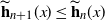 $\mathbf{\widetilde h}_{n+1}(x) \le \mathbf{\widetilde h}_{n}(x)$
for all
 $x \in X$
, we ahve
 $G_{\boldsymbol{\nu}}(\mathbf{\widetilde h}_n|x) = \mathbf{\widetilde h}_{n+1}(x)\le \mathbf{\widetilde h}_{n}(x)$
for all
 $x \not \in D$
. This implies that
 \begin{align*} \mathbb{E}_{\boldsymbol{\nu}}^x[\mathbb{E}_{\boldsymbol{\nu}}^x[t^{E_{n+1}(D)} \mid \mathcal{F}_1]] & = \sum_{f \in S_X} \nu_x(f) \prod_{y \in X}\mathbb{E}_{\boldsymbol{\nu}}^y[t^{E_{n}(D)}]^{f(y)} \\ & = G_{\boldsymbol{\nu}}(\mathbf{\widetilde h}_n|x) = \mathbf{\widetilde h}_n(x) \wedge G_{\boldsymbol{\nu}}(\mathbf{\widetilde h}_n|x). \end{align*}
We observe that
 $\mathbf{\widetilde h}_{0}=\mathbf{h}_{0}$
, since
 $\mathbb{E}_{\boldsymbol{\nu}}^x[E_0(D)] = 1_{x \in D}$
for all
 $x \in X$
; moreover, the sequences
 $\{\mathbf{\widetilde h}_n(x)\}_{n \in \mathbb{N}}$
and
 $\{\mathbf{h}_n(x)\}_{n \in \mathbb{N}}$
satisfy the same recursive equation, so
 $\mathbf{\widetilde h}_n=\mathbf{h}_n$
for all
 $n \in \mathbb{N}$
. This yields
 \begin{align*} \mathbb{E}_{\boldsymbol{\nu}}^x[t^{ 1_{L(A)>0}}] \ge \mathbb{E}_{\boldsymbol{\nu}}^x[t^{E(D)}] = \lim_{n \to +\infty} \mathbf{\widetilde h}_n(x) = \lim_{n \to +\infty} \mathbf{h}_n(x) = \mathbf{h}_\infty \ge \mathbf{v}_\infty. \\[-35pt] \nonumber \end{align*}
Proof of Lemma
4.2. Consider, as in the proof of Theorem 4.1(i), the space-time version
 $\{\eta^\mathrm{st}_n\}_{n \in \mathbb{N}}$
of the process. Clearly,
 $ \limsup_{n\to+\infty}\big\{\sum_{y\in A_n}\eta_n(y) > 0\big\} = \mathcal{S}^\mathrm{st}\big(\bigcup_{n\in\mathbb{N}}(A_n\times\{n\})\big) $
, where
 $\mathcal{S}^\mathrm{st}(\! \cdot \!)$
is the survival event of the space-time process. Recall that, for all
 $A \subseteq X$
,
 $\mathbf{q}^{\boldsymbol{\mu}}(x, A)=\mathbf{q}^{{\boldsymbol{\mu}}^\mathrm{st}}((x,n), A \times \mathbb{N})$
and
 $\mathbf{q}^{\boldsymbol{\nu}}(x, A)=\mathbf{q}^{{\boldsymbol{\nu}}^\mathrm{st}}((x,n), A \times \mathbb{N})$
for all
 $(x,n) \in X \times \mathbb{N}$
. (i) and (ii) follow from Theorem 4.1 applied to the space-time process. (iii) follows from (ii) by noting that
 $\limsup_{n \to +\infty}\big\{\sum_{y \in A_n}\eta_n(y)>0\big\} \subseteq \mathcal{S}(X)$
.
Acknowledgements
The authors are grateful to Elisabetta Candellero for useful discussions. They acknowledge support by INdAM–GNAMPA.
Funding information
There are no funding bodies to thank relating to the creation of this article.
Competing interests
There were no competing interests to declare which arose during the preparation or publication process of this article.


