1 Introduction
Much of the academic literature on performance measurement has focused on the persistence of returns or on the market timing abilities of managers of US mutual funds. This work has its roots in the early work of Jensen (Reference Jensen1968) and has been extended by Carhart (Reference Carhart1997) and Wermers (Reference Wermers2003), among many others. On the whole, the results of the vast majority of the studies in this area suggest that managers of US mutual funds neither display market timing ability, nor can they perform on a consistent basis over time. In the UK, studies by Blake and Timmermann (Reference Blake and Timmermann1998) and by Giles et al. (Reference Giles, Wilsdon and Worboys2002) find that positive performance persistence is absent amongst managers of UK mutual funds (known as unit trusts in the UK), though studies do indicate that negative performance persistence is common.
Our focus in this paper is on the performance of managers of UK pooled pension fund assets. Far fewer studies with respect to this aspect of the investment management industry have been conducted. Given the importance of the UK's occupational pension industry, it is perhaps surprising that so little work has focused on the performance of the fund managers charged with managing these assets. According to the last ONS release on the issue, the market value of the long-term assets held by the UK's pension funds is just over £800bn. At the same time, the pension assets that comprise these pooled funds had a market value of around £400bn (BNY Russell Mellon CAPS survey). This means that they account for around half of all pension assets in the UK. The need to focus on this important industry is perhaps even more crucial at the moment, given that the vast majority of defined benefit (DB) scheme's are in deficit. Watson Wyatt estimated that the combined deficit of the UK's defined benefit pensions industry is £130bn, which implies that the average UK scheme is now facing a deficit of around 15%.
Some studies have been conducted that look at the performance of individual pension schemes. Brown et al. (Reference Brown, Draper and McKenzie1997) investigate the performance persistence of UK pension fund managers.Footnote 1 Using a sample of 232 individual company pension schemes between 1986 and 1992 and another consisting of 409 funds from 1986 to 1992 that retained the same managers over these samples, Brown et al. conclude that there was limited evidence that the managers were able to achieve persistent performance. A result broadly in keeping with persistence studies conducted using alternative fund manager universes.
Bauer and Frehen (Reference Bauer and Frehen2008) analyse the net equity performance of US pension plans between 1992 and 2004. They find that the excess return generated by the fund managers was close to zero, but that it was superior to the performance of mutual funds. This superior performance did not seem to be due to better stock picking or to superior market timing skills by the US pension plan managers. Instead, the authors conclude that pension plans were less subject to hidden agency costs than their mutual fund manager colleagues. For example, the authors postulate that pension scheme clients have greater monitoring capacity than each individual investor in a mutual fund (unit trust).
In another related study, Blake et al. (Reference Blake, Lehmann and Timmermann1999) examine the asset allocation decisions of 364 individual, UK company pension schemes, using data that spanned the period from 1986 to 1994. The criterion they use in identifying the sample is that each fund should have been managed by the same manager over this period, and that this manager should also have been responsible for the asset allocation of the fund over this uninterrupted period, in other words these were balanced mandates. Using this sample, Blake et al. find ‘surprisingly’ little variation in the performance of these schemes, or in the strategic asset allocation decisions that they made over time. In addition, they find that the vast majority of time variation in returns was due to the strategic asset allocation decisions; very little of the variation was due to stock selection. They conclude that the empirical regularities that they observe were most likely due to the legal and economic environments under which these managers operated; for example, the fact that fees were paid on the basis of assets under management rather than on performance. Perhaps their most damning conclusion is that ‘most funds Footnote 2would have been better off with their strategic asset allocation decisions placed in passive index funds' rather than paying for active fund management.
Using the quarterly returns on a much larger sample (2,175) of segregated UK pension schemes spanning the period from 1983 to 1997, Thomas and Tonks (Reference Thomas and Tonks2001) investigate the performance of UK equity portfolios managed by investment managers in contrast to the performance of the balanced portfolios investigated by Blake et al. Thomas and Tonks' conclusions are consistent with those of Blake et al. The variety of techniques used to assess the quality of fund performance all suggest a very narrow cross-sectional dispersion in returns, which suggests that the managers were all ‘closet trackers’. They also conclude that, on the whole, there were negative returns both to selectivity and to market timing.
Finally, Tonks (Reference Tonks2005) suggests that the results of Brown et al. and of Blake et al., might suffer from survivorship bias, since both studies impose the restriction that the pension scheme examined should have the same manager over the sample period. Instead, Tonks looks at the performance of pension funds, irrespective of whether the management changed over the 1983 to 1997 sample period used. Examining the performance of 2,175 UK equity funds over this sample, Tonks finds evidence to suggest that there was indeed performance persistence, at least at the one-year horizon.
The poor performance of actively managed funds – both in the retail and institutional space – that has been reported in numerous studies suggests that investors should perhaps consider investing in passive vehicles rather than seeking to outperform the market by using actively managed vehicles. However, first even a very efficient passive investment technique will underperform the market index by the amount of the fees (though these can be very low for institutional pooled vehicles). And, second, some passive products are less successful than others at tracking their chosen financial market index. Svetina and Wahal (2008) show that passive investments, such as ETFs, can sometimes exhibit substantial tracking error and hence can underperform the target index. This means that choosing the right passive fund – or fund manager with the best tracking skills and techniques – may require some skill too.
In this paper, we investigate the ability of the UK's active pension fund managers to generate alpha for their clients and their ability to time the market. By ‘market timing’, we mean the ability of the manager to increase the risk exposure in the portfolio ahead of a rise in the market and to reduce it ahead of a decline in the market. A fixed-income fund manager could be said to be able to time the market in this sense by increasing the overall duration of the fund as yields generally fall, and reducing it as yields rise across the market. For an equity fund manager, the equivalent skill would be to increase the ‘beta’ of the fund ahead of a rally in equities and to reduce it as equities fall in value.
The evidence for successful market timing amongst mutual funds is very weak in the US and UK. Jiang (Reference Jiang2003) and Cuthbertson et al. (Reference Cuthbertson, Nitzsche and O'Sullivan2009) find no evidence that mutual fund managers can successfully time the market using monthly data for the US and UK respectively.
However, one issue with regression-based market timing models is the low power of the tests when monthly data are used. Bollen and Busse (Reference Bollen and Busse2001) show that the evidence for market timing can be influenced by the cash flows into and out of the fund. They argue that the daily cash flows of mutual funds tend to be positive when the market is rising, and hence that a better gauge of fund manager' market timing ability can be ascertained using daily data. While this may be true for mutual fund investments, it will be less relevant for pension fund investments. The investment committees of most trustee boards generally meet no more frequently than quarterly, so cash flows are more predictable and less sensitive to immediate market conditions. However, another implication of Bauer and Frehen's results is that the performance of pooled retail products (mutual funds and unit trusts) may be different to that of institutional pension funds.
The alternative focus of this paper – on pooled pension funds, rather than on pension schemes – reflects a change in the style of pension fund management over the last 20 years or so. Over this period, pension funds have made increasing use of these pooled funds offered by investment managers. Because of this, the performance of these funds is now of much more relevance to pension fund trustees than would have been the case during the sample periods studied by previous authors. In investigating this aspect of the industry it also means that we do not have to be concerned about changes in the fund management houses since, by definition, they do not change over time. In addition, our results encompass the turbulent equity market periods following the collapse of the high-tech bubble in 2000, whereas data used in previous studies end prior to this period.
The rest of this paper is organized as follows. In Section 2, we describe our data and calculate portfolio performance statistics; in Section 3 we outline the methodology that we employ to investigate the market timing ability of UK pension fund managers; we present the results of the market timing tests in Section 4; and, finally, we conclude the paper in Section 5.
2 Fund data and performance statistics
Because pension funds are exempt from taxation in the UK, the funds studied in this paper have been designed to match the specific legal and tax requirements of pension funds. They are not made available to retail investors, although they are made available to certain other institutional investors, such as charities. However, in essence these funds are analogous to the mutual funds made available to retail and other investors, although they are managed separately and are ring-fenced from all other assets that a fund manager might manage, either on their own behalf or for any third parties.
The Russell Mellon CAPs survey is the industry-standard source for performance information for the UK's pooled pension fund sector, and the source of the data for this study. For a fund to be included in the database, it must be available to UK institutional investors. The survey monitors and provides quarterly performance information on the following equity funds: UK, North American, European (ex UK), Japanese, Pacific, and Global/Overseas equities. The purpose of the Russell Mellon CAPs survey is to display the up-to-date performance of each of the various pooled funds by investment category. The returns in the survey are based upon time-weighted rates of return calculated on both a net and gross basis. Returns are calculated both net of fees from the fund offer prices and, where appropriate, income distributions as quoted by the participating fund management companies. Returns are also calculated gross of fees by adding the charges made against the fund back into the net performance record. However, since pension funds are interested in the returns net of fees, we use net rather than gross returns below. Finally, all the returns are denominated in sterling.
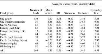
The data consist of the quarterly returns on an initial sample of 734 actively managed pooled equity funds between March 1980 and December 2004.Footnote 3 Of the 734 equity funds, 459 were still available for investment at the end of our sample in December 2004, whereas 275 were classified as dead funds at this date. Only those funds with at least 12 consecutive observations (three years of data) were included in the study of market timing. Of the funds, 593 out of 724 met this criteria. The average number of observations of funds with more than 12 observations was 40.54 quarters, just over ten years. Summary information about the sample is shown in Table 1.
Summary statistics
Only funds with a minimum of 12 observations have been included in the analysis. The maximum number of observations available for each fund has been used. The whole sample period is from June 1980 to December 2004 (99 observations). All statistics are means values of the corresponding statistics for each fund. The number of funds used to calculate the mean are given in column 2. The normality test, reported in the last column is χ2 distributed with 2 degrees of freedom. The critical value at 95% confidence is 5.99.

The summary statistics represent the averages of individual excess fund returns. The quarterly mean excess return of all funds is 0.39% per quarter or 1.56% p.a. It varies considerably between different investment categories, ranging from minus 2.78% p.a. for Japan to plus 5.24% p.a. for UK smaller companies. The variation of the individual fund returns is quite large, averaging 10.78 for all funds. Overall, our data also suggest that the fund returns are not normally distributed and have an average value for the normality test of 6.53 and being as high as 12.10 for the overseas equity category.
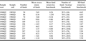
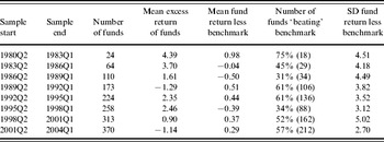
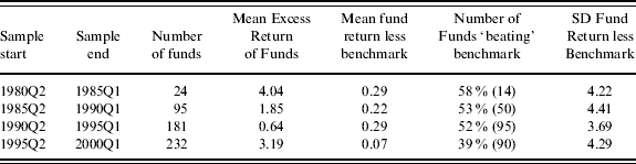
In addition to the summary statistics presented in Table 1, we have also calculated a series of performance-related statistics for the funds in our sample to provide a fuller picture of the risk and return characteristics of these pooled investment vehicles. We believe that this is the first of such analysis of these investment vehicles. In our analysis, we use all of the equity-based pooled funds, as can be seen in Table 1, and these invest in a range of geographic areas. For each geographic region, we have used the appropriate MSCI index measured in pounds sterling as the benchmark. These results are reported in Tables 2, 3, and 4.
Performance of pension funds (1980Q1 to 2004Q4) This table reports the performance of all equity funds in the funds described in Table 1 over a range of non-overlapping investment periods. The performance benchmark for each fund is the appropriate MSCI country/region index. All returns are quarterly returns. The mean excess return in column 4 is calculated as the fund's return less the risk free rate. Column 6 reports the percentage as well as the absolute number of funds (in brackets) over each investment horizon that outperform their benchmarks, while column 7 reports the average standard deviation of fund returns relative to their benchmark.

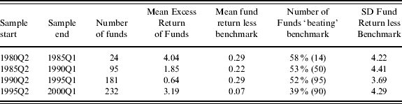
Table 2 details the average performance of these funds, relative to their benchmark over two-, three- and five-year non-overlapping samples, and also relative to the rate of return on cash, represented by the return on a UK government three-month T-bill. For some time periods and investment horizons, these excess returns are positive, suggesting some substantial outperformance on average. However, these excess returns are not statistically significant; the standard deviation of these returns is large as reported in the last column of Table 2.
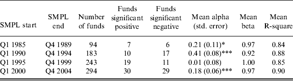
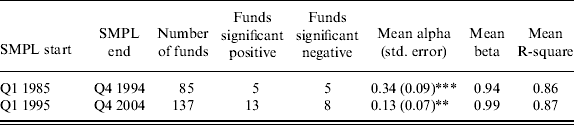
In Table 3, we report the results of CAPM-based regression analysis where the pooled fund returns have been regressed against their relevant benchmark index, over the full 20-year sample and over five- and ten-year sub-samples. We can see that very few funds generate a positive statistical alpha (less than 10% of the funds) – as shown in column 4. Over the full sample, for which we have uninterrupted data on 42 funds, we found that only three of these funds had an alpha which was both positive and statistically significant at conventional levels of confidence. In fact, over each sample we found that almost as many funds produce a statistically significant negative alpha as do a positive and statistically significant one. These results are shown in column 5 of Table 3. The final three columns of this table show the arithmetic mean alpha, beta, and R-squared for all funds from the regression estimates. The average alpha is 0.2% p.a. and is statistically significant from zero with a 10% level of significance and a test statistic of 1.7234. The alphas of four of the six sub-periods are statistically significant at least at the 5% level of significance. The average beta is just under 0.96 for the whole sample period and does not change much for the different sub-periods.
Summary statistics of the mean of CAPM estimation This table reports summary statistics for mean values obtained from CAPM regressions for different sample periods for the funds described in Table 1. The sample periods are indicated in column 1 and 2. In column 3 we report the number of funds available for analysis over each horizon; columns 4 and 5 report the proton of funds with significant positive and negative alphas respectively; while columns 6, 7 and 8 report average alphas, betas, and regression R-squared respectively. The number reported in parenthesis below the ‘mean of the alpha’ is the standard error of this statistic and the stars denote statistical significance at the 1% (***), 5% (**), and 10% (*) levels.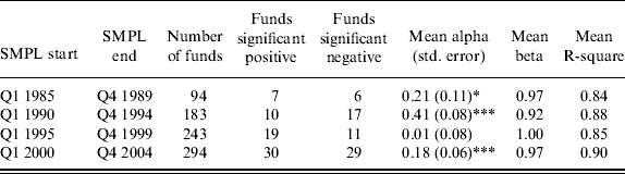
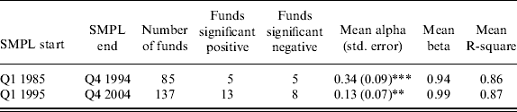

In contrast to most studies of mutual funds, we find that some of the average alphas shown in column 6 of Table 3, particularly over the shorter investment horizons, are significantly positive. However, even when we estimate alphas over a 20-year investment horizon from 1985Q1 to 2004Q4 (see panel C of Table 3), we calculate an average alpha of 0.21, which is significant at the 10% level of confidence. This could be taken to suggest that this part of the fund management industry, unlike the mutual fund sector, does produce positive alpha. But averages can be misleading. Of the 42 funds that comprise this sample, only three had a significant and positive alpha; the remaining 39 funds had no statistically significant alpha at all, or (in two cases) produced a significant, negative alpha. So a pension scheme choosing one fund randomly out of the 42 available back in 1985 had a one in 14 chance of achieving a positive alpha over the following 20-year period. Over the two ten-year sample periods (see panel B of Table 3), this ‘chance’ is one in 17 for the first ten-year sample period, and approximately one in ten for the second ten-year period. The statistical significance of the average alphas in column 6 of the table is, therefore, due to the presence of one or more extreme positive alphas. In other words, the distribution of alphas is skewed to the right. However, having said this, broadly comparable studies of mutual funds tend to find that the number of funds producing negative alphas tends to outnumber those that generate positive alphas.
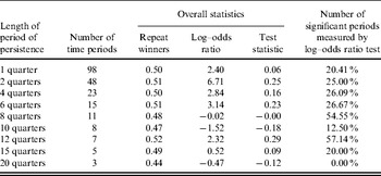
The results in Tables 2 and 3 show that there is limited evidence that these pooled funds outperform their benchmarks on a consistent basis. We extend this analysis now to see how persistent the returns on these funds are. Table 4 reports performance persistence results for these pooled pension funds based on contingency analysis. This analysis requires us to rank all funds by their performance in one period so that they can be divided into winners and losers. We then examine whether they remain as winners/losers over subsequent investment periods. We define a ‘winner’ fund as one that beats its benchmark over the chosen horizon and a ‘loser’ as one that underperforms its benchmark.
Persistence of pension fund performance (contingency tables)
This table reports summary statistics based on contingency analysis of the funds described in Table 1. Funds are categorized as being either winner or losers. A ‘winner’ fund is one that beats its benchmark over the chosen horizon and a ‘loser’ as one that underperforms its benchmark. Column 3 shows how many repeat winners there are over each horizon. Columns 4 and 5 present the log–odds ratio and the test statistic for this ratio, which tests for the presence of persistence in fund returns (see Brown and Goetzmann, 1995). Column 6 reports the proportion of log–odds tests for each individual fund that are statistically significant for specific investment periods.

The number of repeat winners ranges between 44% for the 20-quarter horizon to almost 52% for the 12-quarter investment horizon. Overall, these results indicate that roughly 50% of the funds beat the benchmark, a statistic that one would expect by chance alone.
Brown and Goetzmann (Reference Brown and Goetzmann1995) suggest the following log-odds ratio as a measure of the significance of performance persistence

where w represents a winner fund (i.e. one that has outperformed its benchmark) and l a loser fund (i.e. one that has underperformed). The standard error of the log–odds ratio statistics can be calculated as
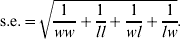
The log–odds ratio is shown in column 5 of Table 4. In column 5, we present the test statistic for the log–odds ratio using the standard error shown above. This test statistic shows no evidence of performance persistence amongst any of the pooled pension funds. We do, however, find some evidence for persistence for some specific time periods. Column 6 reports the proportion of individual log–odds tests that are statistically significant for specific investment horizon analysis. It suggests that there may be certain time periods – that is, certain market conditions – when more funds do better than usual.
3 Parametric and non-parametric tests of market timing
Standard statistical tests for market timing have been proposed by Henriksson and Merton (Reference Henriksson and Merton1981) (HM) and by Treynor and Mazuy (Reference Treynor and Mazuy1966) (TM) for market timing.Footnote 4 The tests are based on regression analysis and are extensions of the CAPM. They assume that the manager's timing ability is dependent upon the relevance of their information about the market. HM estimated the following model

whereas TM used the following regression model

where r i is the excess return of fund i, r m is the excess return on the market, and D is a dummy variable, which takes the value 1 if the excess return on the market is greater than zero, and 0 otherwise. The intuition behind these regression-based tests is that fund managers who do time the market generally increase their exposure to the market prior to the market going up and reduce exposure prior to a decline. This market timing ability is captured by the second term in equations (2a) and (2b).
Abrevaya and Jiang (Reference Abrevaya and Jiang2005) and Jiang (Reference Jiang2003) have suggested an alternative, non-parametric, test for market timing. Based on the CAPM, a fund manager with market timing ability would maintain a higher beta between periods 2 and 3 compared to periods 1 and 2, if r m, 1<r m, 2<r m, 3 for any triplet {r m, 1, r m, 2, r m, 3}. The beta for only two observations is calculated as (r i, t2 – r i, t1)/(r m, t2 – r m, t1). This implies that when the triplets are ordered from the smallest excess market return to the largest value, and the fund manager has market timing ability, one would expect that

Using probabilities, a summary statistic of market timing ability can be expressed as follows (see Jiang, Reference Jiang2003)

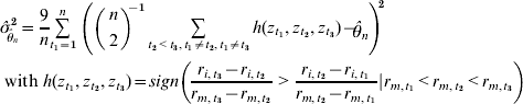
θ measures the probability that the fund return forms a convex relationship with the market return. For a sample, the analogue of θ is a U-statisticFootnote 5, with Kernel of order 3

where n is the number of observations and sign(.) is the sign function taking the values −1, 0 or 1, if the argument is negative, zero, or positive respectively. Abrevaya and Jiang (Reference Abrevaya and Jiang2005) derive a consistent estimator of the standard error of  as
Jiang (Reference Jiang2003) also shows that this unconditional test can be used for a conditional model where r i, t=f i(x) and r m, t=f m(x) and x are some macroeconomic variables which have some forecasting ability, such as the dividend yield, interest rate, or the yield curve. Instead of using r i and r m in equations (4) and (5), we have to use the ‘unexplained excess’ returns. For the baseline model which uses the unconditional excess returns, we would estimate the following regression model: r(i)=a(i)+e(i). The unexplained excess returns are the residuals from a regression model, where the excess returns are regressed on a number of explanatory variables, such as the dividend yield and short-term interest rates. By using these returns, instead of the unconditional excess returns, we can test the success of market timing using risk-adjusted returns.
4 Market timing results
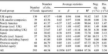
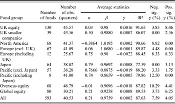
Tables 5 and 6 present the regression results from the Henriksson and Merton and Treynor and Mazuy parametric market timing models. All statistics are averages of all the individual regression results. Market timing is measured by the gamma coefficient, the coefficient on the squared excess return of the market (TM), or the positive excess market return variable (HM). The average explanatory power of either one of those two market timing models is very high with over 87% of the variation explained by the excess market return and the market timing variable. However, for individual funds the explanatory power can be as low as 25%. Comparing the R2 of the market timing models with the CAPM, we see only a slight improvement of the predictive power, less than 5%. The other statistics reported in Tables 5 and 6, are very similar, which indicates that there is not much to choose between these two different tests of market timing. The last two columns report the percentage of funds whose market timing coefficient is statistically significant at the 95% confidence level. Considering all equity funds, the statistics are 4.89% and 3.54% for the Henriksson and Merton model for negative and positive significant gammas respectively. For the Treynor and Mazuy model, the statistics are 7.59% (negative) and 4.05% (positive). Overall, we can conclude that there is not much evidence of successful market timing as these results are only slightly higher than what one would expect due to pure chance (2.5% using the normal distribution).
Parametric market timing test (Henriksson and Merton models)
This table reports the results from the Henriksson and Merton parametric market timing test. All the regression results are averages using the individual regression results. We have used the longest available sample period for each fund for the estimation. Column 3 shows the average length (in quarters) for the different subgroups. The last two columns show the percentage of funds with a significant γ coefficient which indicates market timing. A minimum number of 12 observations were required in order for the fund to be included in the analysis.

Parametric market timing test (Treynor and Mazuy models)
This table reports the results from the Treynor and Mazuy parametric market timing test. All the regression results are averages using the individual regression results. We have used the longest available sample period for each fund for the estimation. A minimum number of 12 observations were required in order for the fund to be included in the analysis.

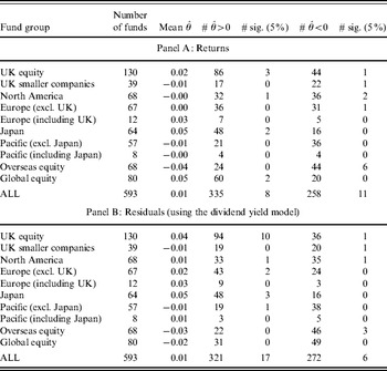
The results from the non-parametric market timing test as suggested by Jiang (Reference Jiang2003) are reported in Table 7. The results for the unconditional model (i.e. excess returns) and the results from the conditional model, where the conditioning variable is the dividend yield are very similar. Using excess returns 335 out of 593 funds reveal a positive market timing test statistic, but only eight funds are significant at the 95% confidence level. Two hundred and fifty eight funds have a negative test statistic with 11 being statistically significant. This means that less than 5% are significant which indicates that the managers of these funds are not able to time the market. The results from the conditional model using the dividend yield as the conditioning variable are very similar to the results from the unconditional model.Footnote 6 Three hundred and twenty one funds have a positive test statistic, and 272 a negative. The number of statistically significant funds are 17 (positive) and six (negative). This is almost the other way round to when returns have been used, but still within the 95% confidence level.
Non-parametric market timing test
This table reports the results from the non-parametric test proposed by Abrevaya and Jiang (Reference Abrevaya and Jiang2005). Panel A shows the market timing statistic using the returns, whereas panel B reports the results where the test is being performed on the residuals using a dividend yield model. Columns 4 and 6 report the number of funds which show a positive (negative) test statistic. The number of statistical significant funds are being reported in the following columns (column 5 for positive funds and column 7 for negative funds).

Looking at the individual funds, we find that only six funds have a positive non-parametric test statistic θ value, using both the unconditional and conditional non-parametric market timing test. Three of those funds have a statistically significant gamma from both of the regression-based tests. Another fund has a θ test statistic of 1.81 using the non-parametric test and statistically significant statistics using the other three tests. All funds that reveal positive market timing using all four tests are UK equity funds. Four funds, with negative market timing ability, have statistically significant negative values, using both versions of the non-parametric market timing test. Three of these funds also show statistically significant negative γs using the parametric test. None of those funds belongs to the UK equity classification. Overall, our results for UK pension funds are very similar to the findings of Jiang (Reference Jiang2003), who similarly found virtually no evidence of significant market timing amongst a large sample of US mutual funds. The fund managers in our sample do not seem to be able to add value to the funds under their management by timing the market.
5 Conclusions
In this paper, we have presented the first comprehensive performance analysis of the pooled pension funds offered to UK pension schemes in the UK. These vehicles comprise a significant proportion of total defined benefit (and defined contribution) pension assets and therefore they deserve attention. They are the UK pension world's equivalent of the retail sector's unit trusts. Although the performance of UK unit trusts has been undertaken in the past, the performance of their pension industry equivalents may differ for any number of reasons. For example, the returns (income and capital gains) from these unitized, pooled pension funds are not subject to tax. Furthermore, in many investment firms the retail and institutional funds are run by different managers.
First, using a range of different methodologies and tests we find limited evidence of positive performance persistence. The implication of this result is that pension schemes may be better off in the long-term investing in passive investment vehicles with their lower associated fees than those of their active equivalents, that is investing to achieve ‘beta’ and not paying for ‘alpha’ which seems illusive. Second, using the non-parametric test for market timing ability suggested by Jiang (Reference Jiang2003), we find virtually no evidence that the managers of these pooled equity funds can time the market. Our results were not materially affected by the use of a conditional version of the test. These results were confirmed by the more traditional, regression-based tests of market timing ability suggested by both Treynor and Mazuy (Reference Treynor and Mazuy1966) and Henriksson and Merton (Reference Henriksson and Merton1981).
Taken together these results suggest that pension fund trustees looking to enhance the value of scheme assets by choosing actively managed pooled investment vehicles rather than say passively managed equivalents, may ultimately be disappointed with the outcome. The ability to ‘add alpha’ and to ‘time the market’ is a crucial element of adding value to any investment portfolio. We find little evidence here that these pooled vehicles offer such return enhancement.