1. Introduction
Climate change is likely to create important negative effects on Brazilian agriculture. With a large part of Brazil's territory located in tropical and subtropical areas, the country will probably suffer serious setbacks as a result of the increase in temperature, as indicated by the most recent scenarios of the Intergovernmental Panel on Climate Change (IPCC).
The Stern Review (Stern, Reference Stern2007) does not provide information on the impacts of climate change on agriculture in developing countries due to uncertainties in the parameter values related to them. A series of studies in Brazil, however, tried to anticipate the effects of climate change scenarios on agriculture. These studies included those by Nobre and Assad (Reference Nobre and Assad2005), Marengo (Reference Marengo2007) and Pinto and Assad (Reference Pinto and Assad2008). The studies consider interactions between environmental parameters and essentially try to predict the percentage decrease in agricultural productivity and loss in agriculturally viable land area in different regions across the country.
In the international literature, Darwin et al. (Reference Darwin, Tsigas, Lewandrowski and Raneses1995) investigated the economic impacts in agriculture around the world, concluding that temperate areas would gain and tropical areas would lose. FAO (2000), in a partial equilibrium framework, points to positive effects in agriculture in developed countries, in contrast to losses in the developing world, especially Latin America and Africa. Fischer et al. (Reference Fischer, Shah and Van Velthuizen2002), Bierbaum et al. (Reference Bierbaum, Holdren, Maccracken, Moss and Raven2007), Cline (Reference Cline2007), Maddison (Reference Maddison2007), Quiroga and Iglesias (Reference Quiroga and Iglesias2007) and Eboli et al. (Reference Eboli, Parrado and Roson2010) also proposed that possible negative impacts would appear in developing countries. Lobell et al. (Reference Lobell, Burke, Tebaldi, Mastrandrea, Falcon and Naylor2008) and Brown and Funk (Reference Brown and Funk2008) analyzed the impacts on agricultural production worldwide, claiming that vulnerability in food security would increase. Ahmed et al. (Reference Ahmed, Diffenbaugh, Hertel, Lobell, Ramankutty, Rios and Rowhani2009) analyzed the effects on agriculture in Tanzania, and Hassan (Reference Hassan2010) has pointed out the difficulties for climate change policies implementation in Sub-Saharan countries.
Less frequent in the Brazilian literature are studies that try to economically assess climate change scenarios in agriculture. Among them is the study by Pinto and Assad (Reference Pinto and Assad2008), performed in a limited framework that considered only the first-order impact of a fall in agricultural productivity, and did not take into account the interaction between the agricultural sector and the rest of the economy. Other relevant studies on Brazil or different regions of the country using econometric methods are those of Sanghi et al. (Reference Sanghi, Alves, Everson and Mendelsohn1997), which focus on changes in land values; there is also a study by Mendelsohn and Dinar (Reference Mendelsohn and Dinar1999) on the evaluation of technological changes in agriculture in Brazil. Additionally, Margulis and Dubeux (Reference Margulis and Dubeux2010) published a general study that included data on agriculture. All of these studies were conducted in a partial equilibrium framework.
These interactions, however, are likely to be very important. Although primary agriculture and livestock production accounted for only 7 per cent of total value added to the Brazilian economy in 2008, it still accounted for 17.8 per cent of total employment in the country (IBGE, 2004), and this production is the basis for a large food and agricultural inputs industry. Ferreira Filho and Horridge (Reference Ferreira Filho, Horridge, Anderson, Cockburn and Martin2010a) also report that the percentage of unskilled labor in Brazilian agriculture is much higher than in other sectors, which suggests important potential effects on income distribution in agriculture that may result from climate change.
Few other studies have addressed the issue of climate change in a more detailed inter-regional model of Brazil and CGE framework. In a study focusing only on northeastern Brazil, Domingues et al. (Reference Domingues, Magalhães and Ruiz2008) used climate change shocks that were uniform across different agricultural activities. Domingues et al. (Reference Domingues, Magalhães and Ruiz2008) used a dynamic CGE model to analyze the problem, distinguishing between different regions and eight agricultural activities. This study, however, has little detail on the expenditure side of the model, and considers only one representative worker and one representative consumer; there are limitations to this method, because the effects of climate change on income distribution must be analyzed more thoroughly.
The purpose of this paper is to assess the potential economic effects of climate change on Brazilian agriculture scenarios in different regions in a general equilibrium framework. A detailed regional economic database for the year 2005 was built, and it was used to calibrate a CGE model of Brazil. Two different climate change impact scenarios are used in the simulations.
This paper differs from other studies in the Brazilian literature in three aspects. First, by considering detailed shocks by product and region, our scenarios take into account the beneficial effects that would come to sugar cane and cassava production in some forecasts. Second, it highlights the connections between the potential impacts of climate change on agriculture and the labor market, with an inter-regional focus. And finally, it specifies the links between climate change forecasts for agriculture and household expenditures, distinguishing between different household expenditure groups, which are also broken down by region. Our study then details the distributional side of the problem, explicitly outlining the links between individual wages and household incomes and expenditures.
In the following section, we present a concise description of the model used in our analysis. Section 3 explains the methodology used to build the impact scenarios. Section 4 includes the simulation results and, finally, the last section summarizes the main conclusions.
2. The TERM-BR model of Brazil
The model used in our analysis is the TERM-BR model, a CGE model of the Brazilian economy whose theoretical structure is based on previous work by Horridge et al. (Reference Horridge, Madden and Wittwer2005), Ferreira Filho and Horridge (Reference Ferreira Filho, Horridge, Hertel and Winters2006, Reference Ferreira Filho and Horridge2008) and Ferreira Filho et al. (Reference Ferreira Filho, Santos and Lima2010). The model's core databases are the 2005 Brazilian Input-Output table (IBGE, 2004), as well as the Brazilian National Household Survey (Pesquisa Nacional por Amostragens de Domicílios, or PNAD) for the year 2005 (IBGE, 2006a), and the Brazilian Expenditure Survey (Pesquisa de Orçamentos Familiares, or POF) for the year 2004 (IBGE, 2004).
The TERM-BR CGE model is static and inter-regional (bottom-up), and essentially consists of 27 separate CGE models (one for each of the states plus the federal district), linked through the markets for goods and factors. Every region, industry and final consumer combine Brazilian and imported versions of each commodity to produce a user-specific constant elasticity of substitution (CES) composite good.Footnote 1 Household consumption of these domestic/imported composites is modeled through the Linear Expenditure System, while intermediate demand has a Leontief (fixed proportions) structure. Industry demands for primary factors follow a CES pattern, while labor is itself a CES function of 10 different labor types.Footnote 2 These different labor types are classified according to wages as a proxy for skills. The model includes 35 separate sectors (or industries), 14 of which are agricultural and livestock sectors. Export volumes are determined by constant-elasticity foreign demand schedules.Footnote 3
These regional CGE models are linked by trade in goods, which is driven by large arrays of inter-regional trade. These arrays record source region and destination region, the values of Brazilian and foreign goods transported, and the associated transport or trade margins (this data is recorded separately for each commodity).
On the income generation side the 10 different wage classes are assigned to each regional industry in the model. The revenues from other endowments (capital and land rents) are combined with these wages to generate household incomes. Each activity uses a particular mix of the 10 different labor occupations (skills). Changes in activity level change employment by sector and region, which in turn drives changes in expenditure and income distribution. Using the POF data, the CGE model was extended to cover 270 different expenditure patterns, which were composed of 10 different income classes in 27 regions.
An important part of any CGE model behavior is determined by the closure rules, or the rules the model must follow in order to find a new equilibrium after a shock. In our simulations, we adopt a long-run closure granted by the capital mobility assumption. Capital stock in each activity changes endogenously, meaning that it can adjust to the new economic environment in order to equalize the rate of return to capital. Profit-increasing industries must attract capital in order to drive down their rates of return. Land is mobile across the agricultural sectors, also driven by rates of return and a constant of elasticity transformation frontier.
As for the labor market, the change in total employment is fixed at the national level, but labor is mobile between industries and regions, driven by changes in real wages. Labor qualification attributes are determined for each type of worker and are also considered fixed. The initial inter-industry and inter-regional wage differentials, although changing with the changes in relative wages, are not eliminated in the simulations. All the productivity parameters were fixed, except for those in agriculture, which were shocked in the simulations.
Total household consumption, government expenditure and investment by sector were determined by the model itself, while preference parameters were fixed. The changes in government expenditures are considered to be equal to the changes in household expenditures. Capital accumulates by sector to equalize the sectoral rates of return. Investment in each industry and region is determined by profits, but investment only affects current aggregate demand profile, and not current production capacity.
3. Climate change impacts on Brazilian agriculture
The criteria used for simulating the impacts of climate change on agriculture are based on the concept of agriculturally viable areas, or the loss of an area's viability for agriculture due to climate change. The papers from Assad et al. (Reference Assad, Pinto, Zullo, Dias, Costa and Nunes2007), Pinto and Assad (Reference Pinto and Assad2008) and Lobell et al. (Reference Lobell, Burke, Tebaldi, Mastrandrea, Falcon and Naylor2008) are the references for the shocks to agriculture used in our simulations. Among them, the most important study for our purposes is the paper by Pinto and Assad (Reference Pinto and Assad2008),Footnote 4 which presents detailed maps of agricultural land loss in different scenarios.
According to Pinto and Assad (Reference Pinto and Assad2008), the methodology for building such maps is based on the Brazilian Climate Risk Zoning of 2007, which is used as a tool for policy planning. An agricultural area is considered suitable for agriculture if the chances of a harvest success are greater than or equal to 80 per centFootnote 5 for the product under consideration (Nobre and Assad, Reference Nobre and Assad2005). In our simulations, we simply eliminated those areas from production, and we did not allow them to be used for other purposes. Our scenarios, then, are more severe than what would be seen in reality, since some different (though marginal) uses could develop in practice for some of those land areas.
Only the main agricultural activities are included in the scenarios developed by Pinto and Assad (Reference Pinto and Assad2008), who calculate the loss of agriculturally viable areas for eight agricultural activities in Brazil: beans, sugarcane, coffee, cassava, rice, cotton, corn and soybeans. Among these activities, only beans are included in a broad group named ‘other products’ in our model classification, while the others are distinguished individually. These authors also calculated the fall in productivity in the remaining areas; while production would still be possible, these areas would become less productive. Changes in land suitability for livestock use, however, were not calculated in Pinto and Assad's Reference Pinto and Assad2008 study. Livestock accounts for a large share of land use in Brazil and, in this sense, the results we describe are an underestimation. There are still no scenarios available for loss of viability for livestock areas in Brazil.
We simulate two different scenarios for two different time spans: the (IPCC) A2 scenario for years around 2020, and the B2 scenario for years around 2070. This choice is based on the idea of adaptation: the more severe scenario for 2020 means that no adaptation would take place in the short run, while the less severe scenario for 2070 means that some adaptation would take place over time.
The rationale behind this scenario choice is as follows. Scenarios are global and impacts are local. We simulated six scenarios (2020, 2050 and 2070, both A2 and B2) generated in the studies on agriculture in Brazil. Notice that the concentration of GHG around 2020/A2 is less than that around 2070/B2, even if B2 is a more adapted trajectory in comparison with A2 scenarios. This happens due to the longer time span around 2070 (an additional 50 years of concentration in GHG emissions in the atmosphere). Then, 2070/B2 is more impacting than 2020/A2. Along general lines GHG emissions are (in terms of concentration): 2020/B2 < 2020/A2 < 2050/B2 < 2050/A2 < 2070/B2 < 2070/A2. Additionally, in economic terms results from 2020/B2, 2020/A2 and 2050/B2 are roughly equivalent. These results are different from 2050/A2, 2070/B2 and 2070/A2, which constitute a second block of results, in our simulations.
The use of a static model to assess climate change implies that we are comparing the scenarios with the model's base year economy, that is, 2005. A dynamic CGE model would allow the comparison of the scenarios with a baseline for the economy, where the trend would be projected. The construction of a baseline, however, would entail difficult questions by itself. For this reason we have chosen to use the traditional static comparative method, with all the results in percentage change deviations from the 2005 economy. Then, this is vulnerability accountability, in opposition to mitigation or adaption strategies against climate change.
The development of shocks to agriculture in the model was done in several different steps. Initially, we used the maps supplied by Pinto and Assad (Reference Pinto and Assad2008) to identify regions which would lose suitability for agriculture, and organized them by state. This information was compared to a county grid map by IBGE (2009). This comparison allowed us to identify the way each micro-region and state would be affected by each product. Once the loss of areas was identified by the aforementioned process, the variation in land use and production loss by agricultural activity could be calculated using information from the Municipal Agricultural Survey, or the Pesquisa Agrícola Municipal (IBGE, 2006b), which is an annual survey of agricultural areas and production. In some cases, especially in northeastern states located north of the Sao Francisco River estuary, agriculture activity would be unfeasible for most agricultural products. In this case, to avoid a complete elimination of agriculture in those regions, an 80 per cent fall limit in agriculturally viable areas was imposed ad hoc in our calculations.Footnote 6
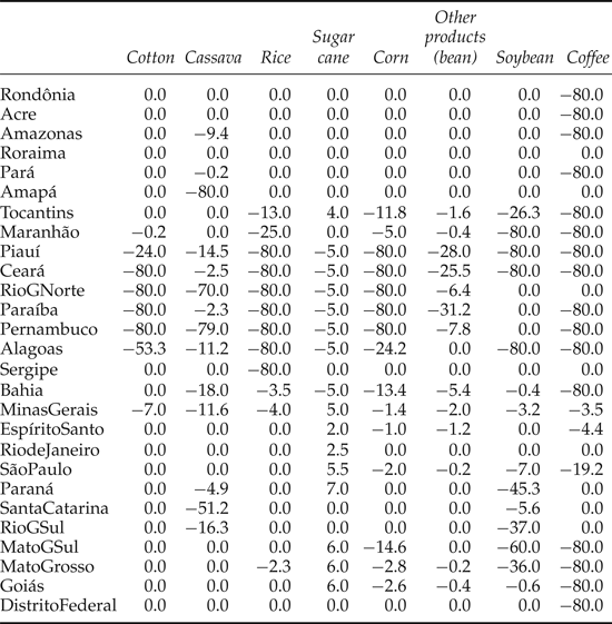
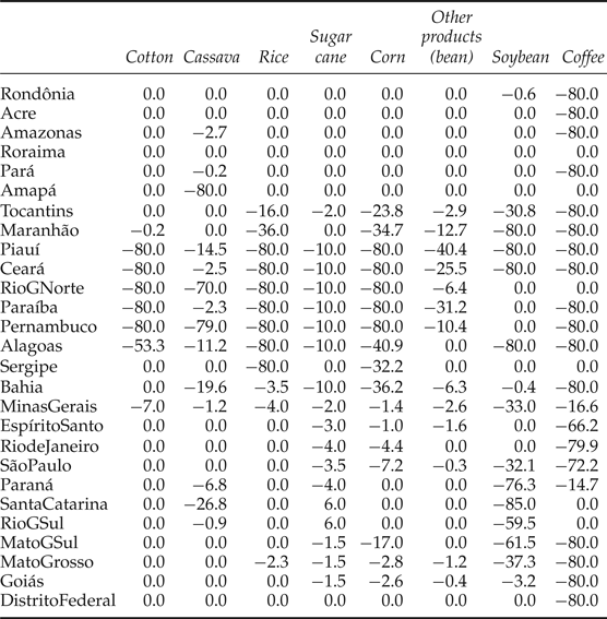
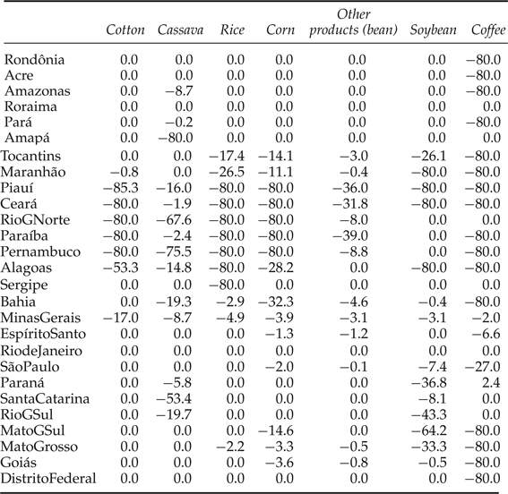
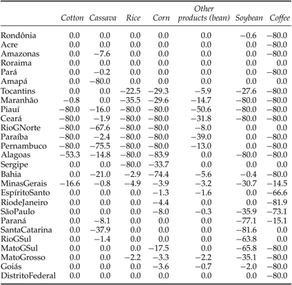
The scenarios include both a decrease in viable land areas and a fall in productivity. The final detailed scenarios, for both land use and production variations, can be seen in appendices A and B, where the regionally aggregated exogenous shocks are displayed. The shocks are particularly severe in the northeastern and center-western regions of Brazil, especially in the cultures of cotton, soybean, rice, corn and coffee. It is important to note that the center-west region is one of the most important soybean-producing regions in the country.
Notice that for the sugar cane crop, there is no direct loss of areas in the scenarios proposed by Pinto and Assad (Reference Pinto and Assad2008); that is to say, a reduction in the area under sugar cane would not be required in the absence of a general fall in total area that would be viable for agriculture. The aggregate fall in land availability, however, would require a decrease in sugar cane areas in the northern and northeastern regions, as well as a slight decrease in the sugar cane area in the southern region, according to the A2/2020 scenario. In the first scenario, there would actually be an increase in sugar cane productivity in some regions (not shown in the table), as a consequence of temperature and CO2 increases.Footnote 7 This increase would benefit the southeastern region of Brazil, where sugar cane production is concentrated.
It is important to note that, despite the strong regional shocks for particular agricultural activities, the southeastern region is considerably less affected than the other regions. This difference is due to the concentration of sugar cane production, which would remain almost completely unaffected by a loss of land viability due to the climate change scenarios. As the data will show, this disparity has important implications for our analysis of income distribution.
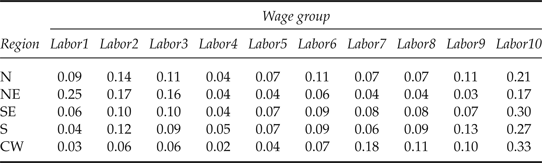
The structure of labor demand in the affected activities is central for this study, and it is analyzed in this section. We will focus our discussion on the labor structure of agricultural activities. The distribution of the aggregate payments for labor in agriculture can be seen in table 1, which displays the percentage of payments for labor that each occupational wage group receives in each macro-region, and which represents the intensity of skill demand in agriculture. In the table, Labor1 stands for the less skilled working group, whereas Labor10 represents the most skilled working group. It can be seen that, in agricultural activities in the northeastern region, there is more labor demand in the less skilled groups than there is in the other regions: the percentage of the three least skilled worker groups in the total agricultural labor bill amounts to 58 per cent in the northeast, but to only 26 per cent in the southeast, and 14 per cent in the center-west. As was seen before, the northeastern and the center-western regions will be more severely affected by the climate change scenarios than the southeast will. The center-west region, on the other hand, has a much more skill intensive labor demand profile in agriculture, with the three highest skills groups representing a 55 per cent share of the total agricultural labor bill in the region.
Labor demand structure in Brazilian agriculture by macro-region (wage bill shares)

Source: Model database.
In the northeast, the bulk of unskilled workers are concentrated in agriculture: the region pays 46.6 per cent of the country's aggregate payments for labor to the first occupational group, and only 8.8 per cent to the higher occupational group, while the richer southeastern Brazil pays only 21.5 per cent to the first occupational group, and 31.8 per cent to the last (more skilled) one. In terms of number of households, the northeast region concentrates 52.7 per cent of total households in the first two poorest income groups.
Finally, when we consider that the poorest workers tend to concentrate in the poorest households, we can conclude that, in the Brazilian agricultural industry, there is a strong possibility that climate change will negatively affect the poorest members of the economy through two main channels: the shrinking of the agricultural labor market in the affected regions; and the increase in the price of consumption bundles, which have the most adverse effects on the poor. These two factors will be discussed separately in the following sections.
4. Results
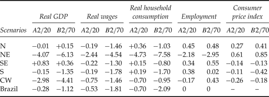
In this section, we present the results of our simulations for the two scenarios, starting with some aggregate variables in table 2. In this table, the results for the 27 states are aggregated in the six administrative Brazilian macro-regions. The heterogeneity of regional impacts becomes evident, with the bulk of the negative effects of the loss of regional gross domestic product (GDP) being concentrated in the northeastern region, one of the poorest regions in Brazil. The second most seriously affected region in terms of GDP loss would be the center-west, the main grain-producing area of Brazil. The negative result for the center-west region is largely determined by changes to the states of Mato Grosso and Mato Grosso do Sul, where soybean production represents a significant share of regional GDP.
Selected macro results (percentage change)

Source: Model results.
Table 3 shows the decrease in projected aggregate land use by macro-region, after scenarios were implemented. It is worth noticing that the numbers in table 3 represent the final changes in land use after the shocks were implemented. For this reason they show changes in land use of all agricultural activities, including those which were not directly affected by the initial exogenous shocks, as is the case of Live Animals. Once the exogenous shocks are implemented, the competition for land determines an adjustment of all agricultural areas in the economy.
Decrease in land use by macro region, two scenarios (percentage change)

Source: Model results.
Southeastern Brazil would benefit from both scenarios in terms of GDP variation. This result is caused by the increase in sugar cane production (in the first scenario), which particularly benefits Sao Paulo state, the main sugar cane producer in Brazil. It is also caused by the increase in the region's labor supply (to be discussed shortly), as well as by the exchange rate devaluation that the model generates. Southeastern Brazil is the most industrialized region in the country, and it sells manufactured products to the other Brazilian regions. A fall in income caused by climate change in the other regions would stimulate exports from southeast Brazil.
The model also points to a moderate decrease in GDP for Brazil: the total effect would be a 1.12 per cent accumulated loss of the Brazilian GDP around 2070 in the B2 scenario, and this loss would include some severe negative effects in different regions. This result illustrates the relatively small share of the affected regions, in terms of production, in the Brazilian economy. It is important to note that the northeast accounts for 12.4 per cent of total Brazilian GDP in the base year, and the center-west accounts for 7.3 per cent. The southeastern region, on the other hand, accounted for 57.5 per cent of Brazil's GDP in 2005. Scenario B2/2070 predicts different changes when compared to the A2/2020 scenario, although the trends observed do not change substantially. The main difference is due to the elimination of the positive effects on sugar cane production observed previously for the southeastern region. In the B2/2070 scenario, sugar cane would also be adversely affected by the increase in CO2 concentration and temperature. As in the A2/2020 scenario, cassava is the product that would benefit most in terms of production.
As table 3 shows, the results confirm the severity of the impacts of these climate change scenarios on the northeastern and center-western regions of Brazil. The southern region is also much more negatively affected in the B2/2070 scenario than it is in the A2/2020 scenario: as climate change progresses, its negative effects will start to have greater impacts on the southernmost regions of the country.
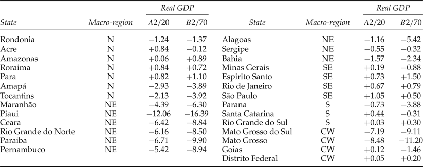
A closer look at a more disaggregated regional level is also possible, and can be seen in table 4, which displays information on GDP variation by state. The macro-region to which each state belongs is in brackets. It can be seen that the GDP losses in individual states are considerably larger in the B2/2070 scenario, with strong losses in some states in the northeastern (NE) and center-western (CW) regions. An example includes the state of Piaui, one of the poorest in Brazil, which would have a 16.39 per cent fall in accumulated GDP around 2070. The GDP loss for the state of Mato Grosso is also noteworthy, reaching an 11.20 per cent decrease around 2070.
Model results, GDP variation, by state (percentage change)

Source: Model results.
Some regional GDP loss results are comparable to those found by Fischer et al. (Reference Fischer, Shah and Van Velthuizen2002), who argued that the drop in production would be concentrated in developing countries. The fall in GDP of some Sub-Saharan African countries would be around 9 per cent, close to the value that was calculated in the Brazilian northeast.
Finally, the losses in GDP projected in scenarios A2/2020 and B2/2070 would amount to R$6.06 (US$ 2.6)Footnote 8 billion and R$24.27 (US$10.4) billion, respectively. For the sake of magnitude comparison, the FAO (2000) points to losses in the range of US$14–142 billion for Latin American countries in the year 2100.
The drop in regional economic activity would trigger important changes in labor markets, with impacts on welfare and income distribution. The effects on labor demand caused by the climate change shocks can be seen in more detail in table 5, in which labor demand variation is found to be disaggregated in the model's 10 occupational groups. These labor groups are classified according to wage groups, representing different labor skills: Labor 1 is the group with the least skilled workers in the model, while Labor 10 includes the most highly skilled workers. As the table shows, labor demand would fall for all labor skill groups in the Brazilian northeast, and for most skill groups in the center-west. The southeast and south of Brazil would see an increase in employment.
Labor demand variation by skill and state (percentage change)

Source: Model results.
Total labor was kept constant in the simulation, which means that the shock would generate an inter-regional labor migration toward the southeast of Brazil. Workers displaced by the drop in economic activities in the affected regions would tend to migrate to the other, less affected regions. It is important to note that this result would represent a change in the recorded migration flows in Brazil, which, in the first half of the last decade, revealed an inversion of a long-observed trend in Brazil. Ferreira Filho and Horridge (Reference Ferreira Filho and Horridge2010b) found that, from the year 2000 on, net migration flows occurred from southeastern Brazil toward northeastern Brazil, inverting the traditional and historical northeast–southeast migration flows.
It is also important to note that center-western Brazil would face a reduction in the employment of more highly skilled workers (labor group 5 and above), and an increase in the employment of the less skilled groups. This predicted change is related to the labor demand composition inside the region's agricultural sector, as well as to the change in product mix after the shocks. Soybean production would be strongly reduced in the region, while cassava production would likely increase. Soybean production is highly mechanized in Brazil, and demands proportionately more skilled labor than cassava, which requires a greater labor demand from the lowest skill groups.
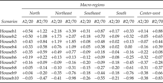
In the model, the change in production composition has impacts on food prices in the economy, leading to distinct consequences for household consumption, depending on each respective expenditure pattern. As mentioned previously, our model distinguishes between 270 different expenditure patterns. The shocks to agricultural production, therefore, would cause a more negative impact on food items, due to both the direct fall in agriculture production and to the indirect reduction in some other industry costs, which would, in turn, be due to the related fall in wages. The model's results can be seen in table 6, which displays the consumption bundle price index variation by income group and macro-region. In the table, Househ1 refers to the lowest household income group, and Househ10 refers to the highest household income group.
Consumption bundle prices variation (percentage changes)

Source: Model results.
The results in table 6 are a combination of the particular regional consumption bundles, and of each region's product price variation. In general, the service sectors account for the majority of household expenses from group 7 to group 10. Essentially, but not exclusively, the smaller variation in the expenditure bundle of the richest households is due to the service sector's price variation. This sector is one of the largest absorbers of unskilled labor in the Brazilian economy, and tends to hire labor as wages come down as a result of shrinking agricultural sectors in the affected regions.
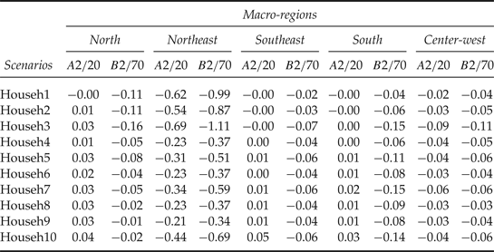
The changes in welfare generated by the shocks can be better summarized by money metric welfare variation indexes, as is the case of the Hicksian Equivalent Variation (EV), shown in Table 7 as a share of each state's GDP. As can be seen, Househ3 in northeast Brazil, for example, would face a welfare loss equivalent to 0.69 per cent and 0.99 per cent of regional GDP, respectively, in scenarios A2/2020 and B2/2070. Again, even though spread all over the economy, welfare losses are highly concentrated in northeast Brazil.
Equivalent variation change as a share of regional GDP

Source: Model results.
Finally, we performed a sensitivity analysis with three key parameters in the model: the elasticity of substitution between primary factors, the elasticity of substitution between labor types, and the imported/domestic elasticity of substitution, with values 20 per cent lower and higher than the ones used in the simulations. The results for national GDP are virtually the same as the ones observed in the main simulation. Even in regional terms the differences in results are not high and do not change the general conclusions of the main simulation. Regional GDP variation in northeast Brazil, for example, ranged from −3.85 to −4.01 per cent around 2020 (−4.07 per cent in the main simulation) and from −5.55 to −7.08 per cent around 2070 (−6.13 per cent in the main simulation). The same can be said about the EV variation. Taking as an example the EV as a share of GDP for the poorest household in northeast Brazil, the value ranged from −0.57 to 0.67 around 2020 (−0.62 in the main simulation) and from −0.91 to −0.15 around 2070 (−0.99 in the main simulation).
Our results, therefore, reinforce the conclusion that climate change impacts on agriculture in Brazil would affect the poorest members of society most dramatically, a result which agrees with results from the literature worldwide, as seen before.
5. Conclusion
Our results show that, in spite of the severe scenarios on land loss and agricultural productivity analyzed in this paper, climate change impacts on Brazilian agriculture would have a relatively small economic impact on the Brazilian economy in aggregate terms, in the long run. The negative shocks to land use and production are concentrated in regions where the percentage of agriculture from the national total is relatively small, leading to small GDP losses in aggregate terms. The really severe consequences, however, would appear at the regional level, and this paper highlights the importance of regional divisions when approaching such phenomena in large countries such as Brazil. Our results make a strong case for losses that would be concentrated in the poorest regions and, more specifically, for the poorest workers and households in those regions. This outcome is determined by labor composition in the agricultural sector in the most severely affected regions, as well as by the composition of the consumption bundle of those households. This prediction raises at least two lines of concern for public policy considerations, and these causes for concern are intertwined.
First, through the impacts on the agricultural industry, climate change has the potential to undermine the efforts made by the Brazilian government in the last decade to reduce poverty in the poorest regions of the country, precisely those where the most serious effects were seen using the scenarios simulated in this paper. Climate changes would create new challenges for poverty alleviation in Brazil. The second important point to consider is the potential surge of new waves of low-skilled migrants toward southeastern and southern Brazil. From a public policy standpoint, this potential migration is a key issue. The northeast–southeast waves of labor migration in Brazil in the past, which peaked in the 1970s and 1980s, supplied labor for industrialization and agriculture in the south-southeast and center-west of Brazil, but these waves also generated numerous social problems in the big cities that have yet to be resolved. Public policies managed to generate a faster rate of growth in northeastern Brazil in the last decade. The rate was above the national average and caused a decentralization of economic activity that resulted in a faster economic convergence among the Brazilian states. This decentralization was certainly an important (but not the only) element in the appearance of a net migration flow from the southeast toward the northeast of Brazil, and in some ways it alleviated congestion problems in the main cities. Trying to anticipate these effects and designing compensatory policies should be ranked high on the Brazilian research agenda.
And, finally, we recognize that the path of the adjustment to the climate change shocks can be important, but this analysis would require a dynamic model. Future research on the topic should be ranked high on the research agenda.
Appendix A
Supply shocks (production value) in the scenario 2020/A2 (percent changes)

Supply shocks (production value) in the scenario 2070/B2 (percent changes)

Appendix B
Land use changes (exogenous shocks) in scenario 2020/A2 (percent changes)

Land use changes (exogenous shocks) in scenario 2070/B2 (percent changes)