1.1 Objects of interest and scope

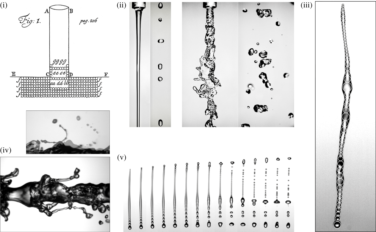
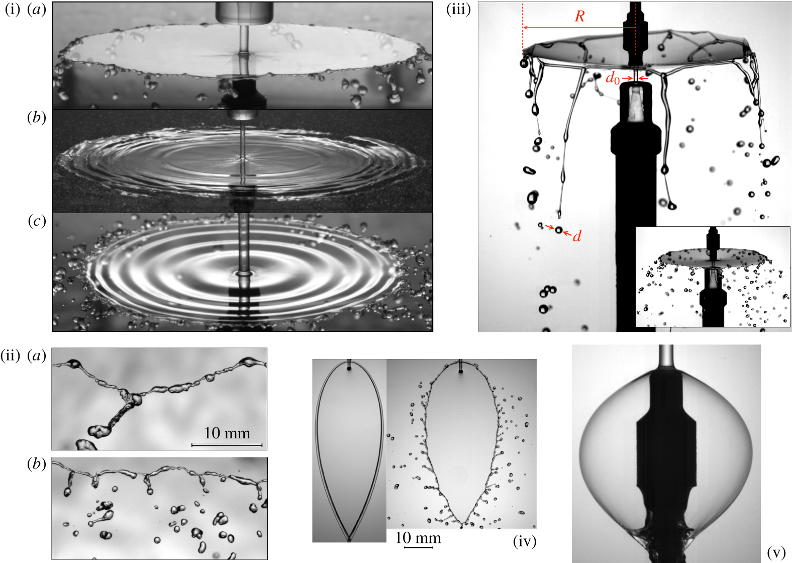
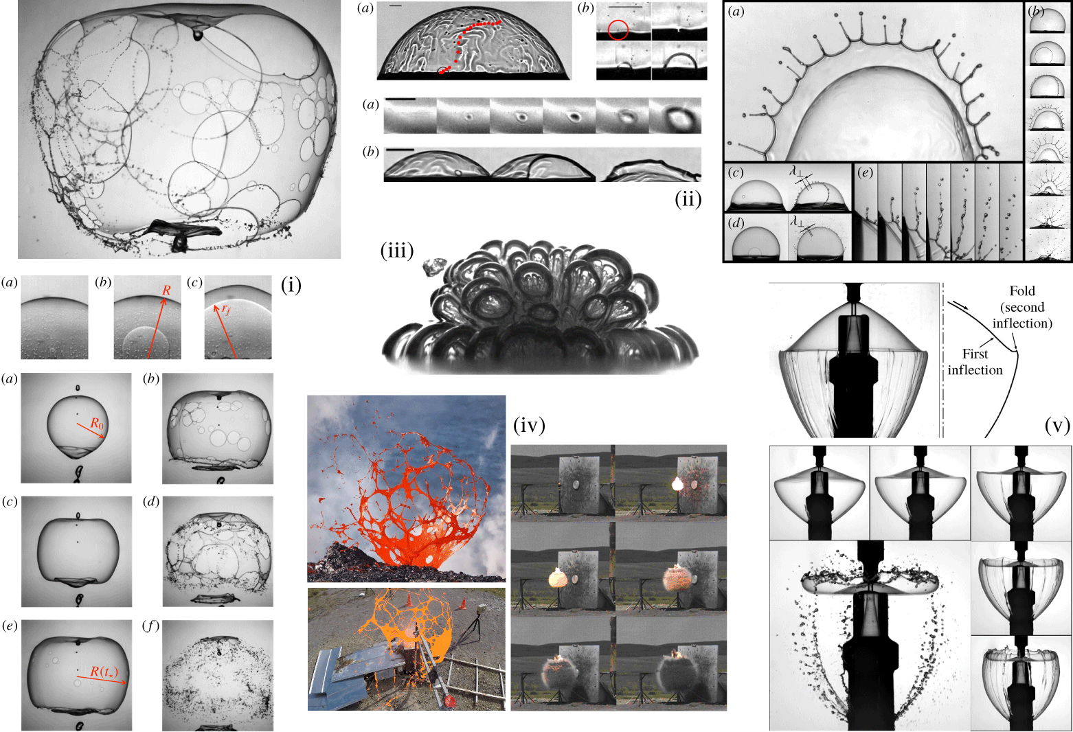
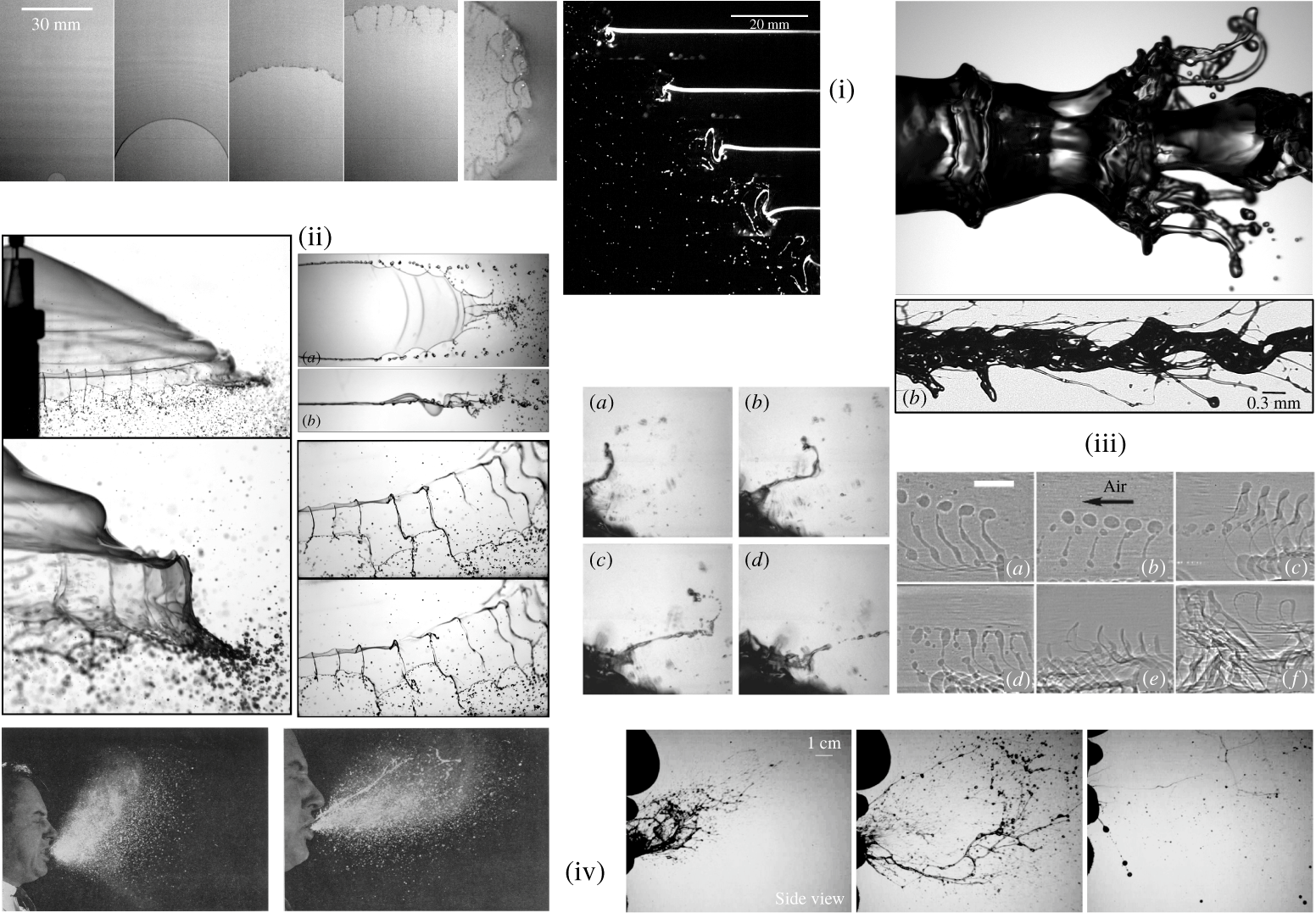
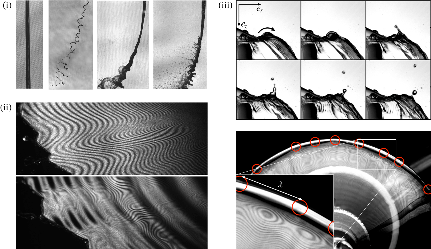
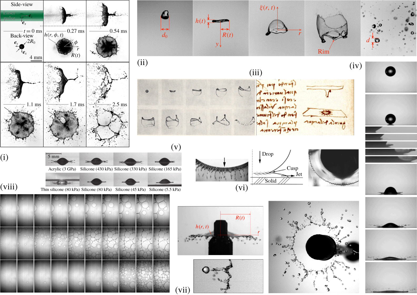
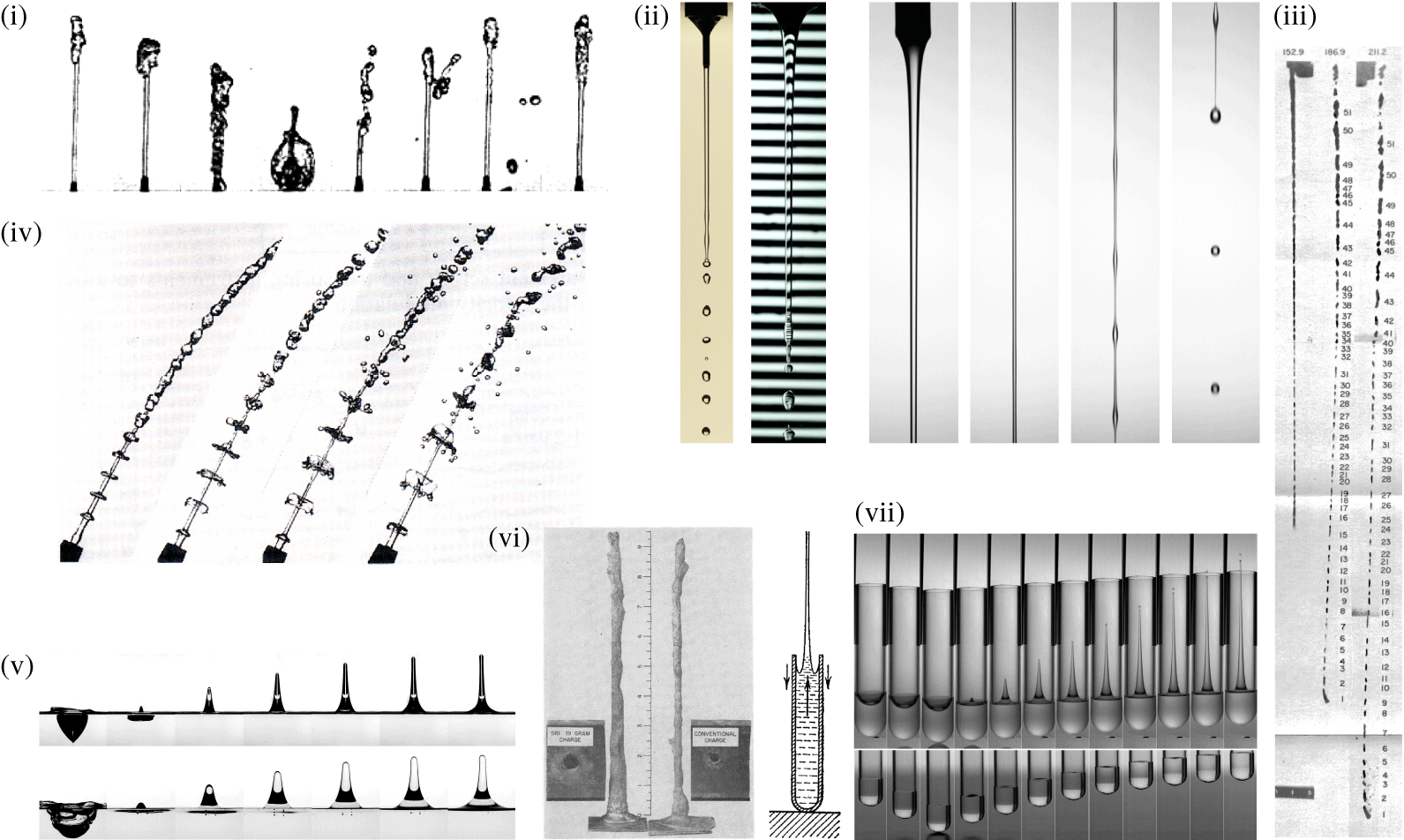
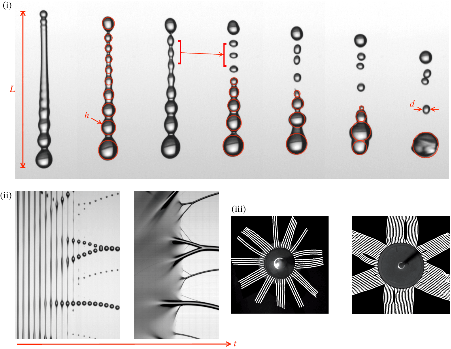
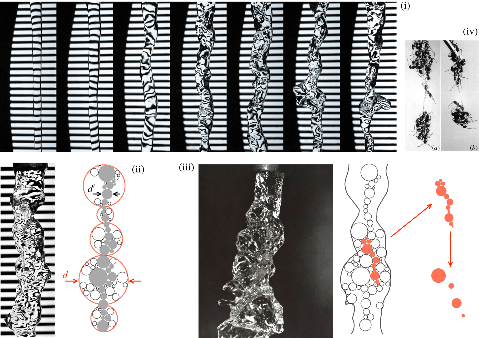
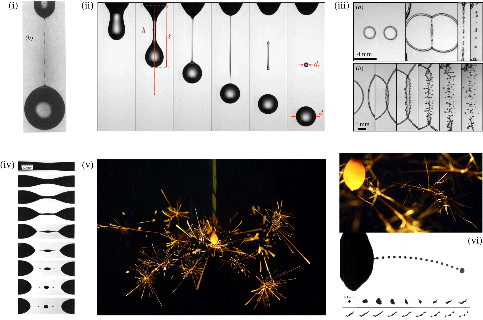
The subject matter, illustrated in figure 1, will be concerned with liquid sheets, shells, holes, jets and ligaments, those which ultimately break into stable fragments, namely the final drops. Since these ligaments, kind of elongated, finite sized rough columns will be shown to be the ‘sinews’ of liquid fragmentation (Villermaux Reference Villermaux2007), their formation will be tracked, and described along with the instabilities giving birth to them in a variety of different situations with applications ranging from liquid propulsion, agricultural spraying, to the formation of ocean spray, raindrops and human exhalations by violent respiratory events etc. … It will be shown that their dynamics, and final outcome, results from a trade-off between cohesion and fragmentation.

Figure 1.

Rome, Piazza del Popolo, the lions of the central fountain expectorate a turbulent water sheet. Random velocity fluctuations and possible bubbles inclusions in the liquid nucleate holes which, driven by surface tension, grow and merge, leaving the sheet as a set of connected ligaments. These corrugated ligaments further breakup into a collection of disjointed droplets broadly distributed in size.

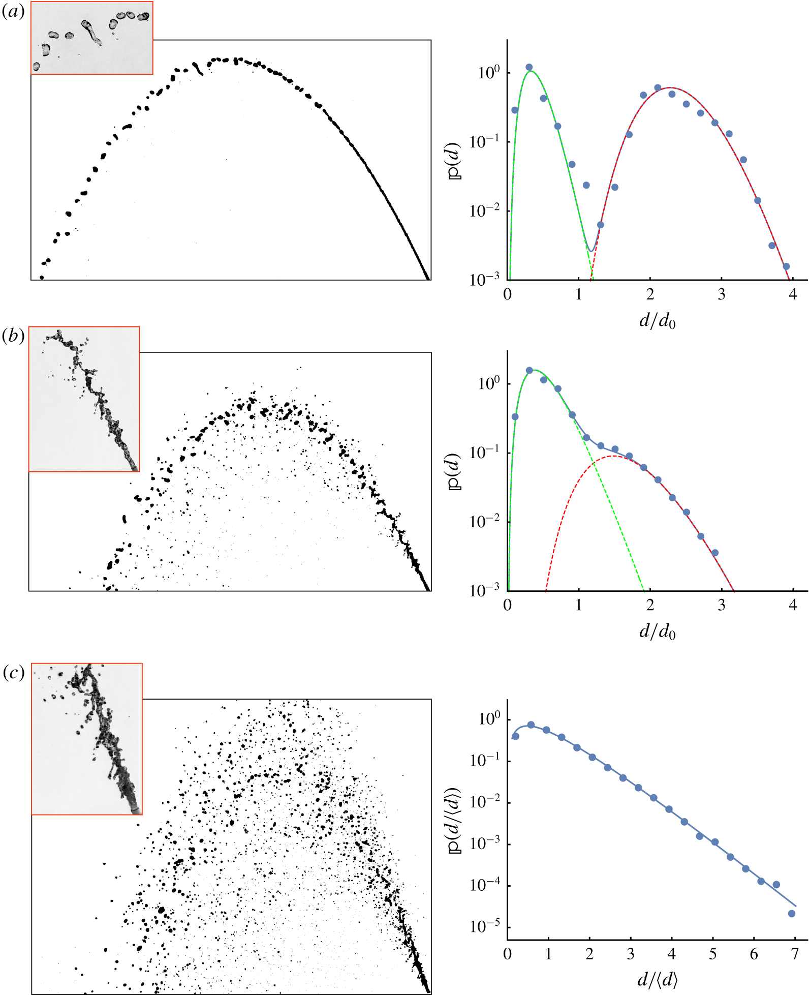
Attention will be paid in each case to understanding the overall drop size distribution, for at least two reasons: first because a satisfactory understanding of a physical phenomenon requires its complete statistical description, particularly when it is non-trivial, and second because most applications urge us to do so, as we explain next.

1.2 Distributions rather than just averages

We list below a number of situations taken from various fields showing the importance, in fragmentation, of understanding or controlling the overall drops size distribution, rather than just a mean size.

(i) Liquid propulsion, combustion, drying: fragmentation is a mandatory step in various industrial processes for example in furnaces, liquid propulsion engines or drying facilities, contexts where it is usually called atomization (i.e. literally, down to the atom size). Although produced in a swarm with other droplets densely packed in space at the atomization nozzle, it is nevertheless often the fate of an individual liquid droplet which is of practical interest: the length of a liquid propulsion combustion chamber, or the height of a drying tower depends on the distance from the injection nozzle for the last, biggest droplet of fuel, or solvent, to evaporate, burn (Marble Reference Marble1964) or solidify (Yule & Dunkley Reference Yule and Dunkley1994). Conversely, fine droplets burn too soon after their formation, and may damage the injectors. A better control of the fuel droplet size distribution at injection is one of the ways to improve car engine consumption (Taylor Reference Taylor2008).

(ii) Agricultural spraying, snow lances, painting and printing industry, dust control: spray drift is a major concern in agriculture. Standard flat fan atomizers used to spray fields with fertilizers and pesticides produce broad drops sizes distributions, with a notable fraction with diameter below 100 μm (called ‘fines’) likely to be swept by the wind, reaching the farmer’s neighbour’s field who may not like it, or the river next to it (Hewitt Reference Hewitt2000; Kooij et al. Reference Kooij, Sijs, Denn, Villermaux and Bonn2018). Strategies to reduce their relative number are the subject of active research (Hilz et al. Reference Hilz, Vermeer, Cohen Stuart and Leermakers2012; Vernay, Ramos & Ligoure Reference Vernay, Ramos and Ligoure2015a). The biggest droplets, however, soon fall by their own weight, are too heavy to hook on plants leaves or rebound on them, splash like raindrops do, favouring plant-to-plant contamination (Gilet & Bourouiba Reference Gilet and Bourouiba2015). Snow lances, whose popularity is indexed on the progress of global warming, suffer from the same flaw: light snowflakes from tiny droplets wander aloft, missing the targeted ski slope, while big droplets fall on the ground before freezing, finally producing undesired ice. For similar reasons, the rotary atomizers used in the automotive painting industry produce many droplets that fail to reach the car bodies they are supposed to coat (Wilson et al. Reference Wilson, Grib, Ahmad, Renfro, Adams and Salaimeh2018). Dust particles are routinely removed from air by sprays with a capturing efficiency depending critically on the droplet sizes (Swanson & Langefeld Reference Swanson and Langefeld2015). The formation of undesired small satellite droplets causes notorious difficulties in inkjet printing (Wijshoff Reference Wijshoff2010; Basaran, Gao & Bhat Reference Basaran, Gao and Bhat2013).

(iii) Geophysics, planetary sciences, precipitations: the Earth was built by high-energy impacts of planetesimals with metallic cores of their own. The composition of the Earth’s mantle depends critically on the time offered to metal–silicate chemical equilibration as the impactor material settles towards the Earth’s core. It fragments very much like raindrops form as they fall from clouds in the atmosphere (Villermaux & Bossa Reference Villermaux and Bossa2009), producing broad size distributions (Marshall & Palmer Reference Marshall and Palmer1948). Efficient equilibration is achieved with smaller fragments allowing fast metal–silicate mass transfer, while the fate of bigger ones is to accumulate in the – therefore iron-rich – core. The overall planet chemical composition relies on fragmentation (Deguen, Landeau & Olson Reference Deguen, Landeau and Olson2014; Landeau, Deguen & Olson Reference Landeau, Deguen and Olson2014; Wacheul et al. Reference Wacheul, Le Bars, Monteux and Aurnou2014).

(iv) Sea spray: the spray produced by wave breaking in the surf zone, or white caps at the ocean surface, is a superposition of different mechanisms which results in broadly distributed droplet sizes (nanometres to millimetres, see e.g. O’Dowd & de Leeuw (Reference O’Dowd and de Leeuw2007) and Veron (Reference Veron2015)). If they all contribute to the global air–sea exchanges, the fate of each droplet in this distribution is not identical: the smallest aerosols are long lived in the atmosphere, carry salt and diverse chemical/biological substances (Cochran et al. Reference Cochran2017; Pietsch et al. Reference Pietsch, Grothe, Hanlon, Powers, Jung, Ross and Schmale2018) over large distances inland while the biggest spume droplets carry momentum, heat and produce moisture by evaporation, feeding hurricanes for example, before settling by gravity.

(v) Exhalations, disease transmission, seeding: human exhalations like coughing or sneezing produce a broad spectrum of droplet sizes, possibly carrying pathogens and thus mediate disease transmission (Pasteur Reference Pasteur1861; Flügge Reference Flügge1897; Winslow & Robinson Reference Winslow and Robinson1910; Duguid Reference Duguid1946). This well known fact is currently re-examined in the light of modern methods and ideas (Turner, Jennison & Edgerton Reference Turner, Jennison and Edgerton1941; Bourouiba, Dehandschoewercker & Bush Reference Bourouiba, Dehandschoewercker and Bush2014). The contamination radius of an infected coughing individual is the distance needed for the last liquid droplet exhaled from his mouth and staying aloft in air to evaporate (Wells Reference Wells1955), but it is not clear which are the nastiest most long-lived droplets in the exhaled spectrum; it has been suggested that the finest are the nastiest, through a collective evaporation delay mechanism (Villermaux et al. Reference Villermaux, Moutte, Amielh and Meunier2017). Fungi reproduce by ejecting encapsulated seeds of different sizes, the biggest, heaviest and thus farthest reaching ones being responsible for substrate exploration, while the smallest exploit the substrate in the immediate emitter vicinity (Ingold Reference Ingold1971). These airborne spores, like pollens, can be carried over long distances, crossing oceans (Hirst, Stedman & Hogg Reference Hirst, Stedman and Hogg1967; Aylor Reference Aylor2017).

(vi) Medicine, forensic science, inhaled drugs, scents: some therapies rely on inhaled aerosols carrying drugs which should be embedded in particles whose size is critical to escape from the lung’s natural clearance mechanisms. Controlling particles sizes, and density is vital in this context (Edwards et al. Reference Edwards, Hanes, Caponetti, Hrkach, Ben-Jebria, Eskew, Mintzes, Deaver, Lotan and Langer1997). Experts in the forensic technique of blood pattern analysis routinely contemplate blood splats to decipher the circumstances of a homicide. These splats consist of myriads of stains on the floor which are meaningful only when the fragmentation process creating them has been understood (Attinger et al. Reference Attinger, Moore, Donaldson, Jafari and Stone2013). Electronic cigarettes (e-cigs) are efficient, cancer agent free, tobacco smoking alternatives. However, the nicotine-rich aerosol produced by e-cigs has a droplet size distribution appreciably more skewed towards small sizes than the tobacco smoke particles, with a fat tail towards ‘nano’ particles; they are, for this reason, considered as suspect (Glantz & Bareham Reference Glantz and Bareham2018). There is a, yet unexplored, relationship between the way a fragrance spray has been atomized, and the persistence of its scent, admittedly a fascinating question.

1.3 A fragmented world

The examples above suggest that we are indeed living in a fragmented world, in more than one sense. There are other sectors of science where the dilemma between cohesion and fragmentation has been identified as paramount: for example, the survival of colonies of living species is known to be influenced by their habitat fragmentation. While fragmentation is usually believed to have a deterring impact on wildlife colonies because it promotes species competition for limited resources and inbreeding, thus hampering bio-diversity (Betts et al. Reference Betts, Wolf, Pfeifer, Banks-Leite, Arroyo-Rodríguez, Ribeiro, Barlow, Eigenbrod, Faria and Fletcher2019), other aspects like long lasting adaptation to a given small perimeter substrate in an immigration/emigration-free isolation is known to favour persistence (Mac Arthur & Wilson Reference Mac Arthur and Wilson1967; Letcher et al. Reference Letcher, Nislow, Coombs, O’Donnell and Dubreuil2007). In sociology, spatial fragmentation and its cultural corollary have been identified to impede social cohesion, and are considered as a threat to democracy. These topics are, however, out of the scope of this review.

2.1 Founding idea of Laplace (Reference Laplace1805)

The founding idea is due to Laplace (Reference Laplace1805). Liquids rise spontaneously in narrow tubes. Well aware of Newton’s Query 31 (Newton Reference Newton1704), and of the subsequent experimental observations by Hawksbee and Jurin intended to solve this inadmissible exception to the theory of gravitation (see the detailed history in Rowlinson (Reference Rowlinson2002)), Laplace conjectured, a century later, the existence of a central force between nearby ‘molécules’ (or ‘particles’ as Hawksbee called them; this word has to be understood as a synonym of ‘small amount’, for instance, Newton (Reference Newton1687) refers to a particle of time to designate an infinitesimal time increment): two masses $m$ and $m^{\prime }$ distant by $f$ are attracted by a force $m\,m^{\prime }\unicode[STIX]{x1D719}(f)$ with $\unicode[STIX]{x1D719}(f)$ assumed to be very intense at short distance, and evanescent for large separation distances $f$, in Laplace’s notations. This formalism, exposed in his Traité de Mécanique Céleste is directly imported from the one operating for gravitational forces. The work of separation, or binding energy of the particles pair is $u(f)=\int _{f}^{\infty }\unicode[STIX]{x1D719}(f^{\prime })\,\text{d}f^{\prime }$. Lord Rayleigh (1890), in his exegesis of Laplace’s contribution, shows how successive summations provide the attraction from a half-space with density $\unicode[STIX]{x1D70C}$ on a unit mass at distance $z$ from its bounding plane $\unicode[STIX]{x1D713}(z)=2\unicode[STIX]{x03C0}\unicode[STIX]{x1D70C}\int _{z}^{\infty }fu(f)\,\text{d}f$, that the mutual attraction between two half-spaces separated by $x$ is $\unicode[STIX]{x1D703}(x)=\unicode[STIX]{x1D70C}\int _{x}^{\infty }\unicode[STIX]{x1D713}(z)\,\text{d}z$ per unit plane surface area, producing an internal bulk pressure $K=\unicode[STIX]{x1D703}(0)$, and that the separation work of the two planes from contact is $2\unicode[STIX]{x1D70E}=\int _{0}^{\infty }\unicode[STIX]{x1D703}(x)\,\text{d}x$.

Thus defined as an energy per unit surface, what is now called the surface tension of the material or, equivalently, its fracture energy (we will come back to this delicate question in § 11), is related to the hypothesized microscopic force $\unicode[STIX]{x1D719}(f)$ by the celebrated formulae

(2.1)$$\begin{eqnarray}\unicode[STIX]{x1D70E}=\frac{\unicode[STIX]{x03C0}}{8}\unicode[STIX]{x1D70C}^{2}\int _{0}^{\infty }f^{4}\unicode[STIX]{x1D719}(f)\,\text{d}f.\end{eqnarray}$$

Surface tension is a finite quantity provided the force $\unicode[STIX]{x1D719}(f)$ decays fast enough with $f$, and it is not the least of Laplace talents to have embarked in this description without, at the time, an empirical proof of the existence of molecules and ignoring that, more than a century later, quantum mechanics would rationalize the so-called van der Waals forces (Israelachvili Reference Israelachvili1991) by showing that $u(f)\sim f^{-6}$ and that therefore $\unicode[STIX]{x1D719}(f)\sim f^{-7}$, a decay making the integral in (2.1) convergent indeed (Laplace had envisaged, safely, an exponential decay).

2.2 Clausius disgregation (Reference Clausius1862)

Clausius (Reference Clausius1862) created the ephemeral concept of disgregation which he himself soon replaced by the notion of entropy. Clausius wanted to formalize the idea that a body mass exchanging heat or work with an outside source suffers an ‘alteration of arrangement’ of the ‘aggregation state’ of its constitutive molecules:

We would nowadays call disgregation the configurational part of the entropy but it is interesting to note that by ‘dispersed’, Clausius equally meant loosely aggregated (like molecules in a liquid), or completely disjointed (like in a gas). Cohesion, aggregation and fragmentation are thus notions which were thought at this time as parts of the same problem, or at least as having strong inter-relationships.

We have on purpose recalled the early ‘particulate’ description of matter cohesion first to underline its origin as an inspiration from the theory of gravitation and central forces between isolated bodies. It is also possible that Laplace, who knew well the experimental background of the Cambridge group, notably the one of Hawksbee, has been influenced by one of his drawings, reproduced in figure 2, where sizable ‘particles’ are clearly evidenced as the constitutive components of a liquid. And second, because this representation will be useful to understand the dynamics of fragmentation per se, and the origin of the multiplicity in fragment sizes, through considerations à la Clausius where disgregation and aggregation compete on an unstable substrate (§ 9). We examine such an example below.

Figure 2.

(i) A sketch from Hawksbee (Reference Hawksbee1709) where ‘particles’ are clearly singled out as the constitutive components of a liquid, here ascending in a capillary tube. (ii) Breakup of a laminar, falling smooth water jet ($h_{0}=4~\text{mm}$ and $v_{0}=1~\text{cm}~\text{s}^{-1}$) contrasted with the fragmentation of the same, but turbulent jet. (iii) The ‘particulate’ vision of the rearrangements occurring during ligament breakup (Villermaux, Marmottant & Duplat Reference Villermaux, Marmottant and Duplat2004). (iv) Stripping of ligaments at the surface of a water jet sheared by a fast coaxial stream (Marmottant & Villermaux Reference Marmottant and Villermaux2004b). (v) The time lapse of an isolated ligament featuring longitudinal rearrangements as it breakup.

2.3 Fragmentation of a necklace of magnets

In order to see how cohesion and disgregation compete, it is instructive as a starting exercise to work out the caricatural problem of the sudden forced radial expansion of an assembly of attracting particles arranged in a circle: the shatter of necklace of magnets (Vledouts, Vandenberghe & Villermaux Reference Vledouts, Vandenberghe and Villermaux2015, Reference Vledouts, Vandenberghe and Villermaux2016b).

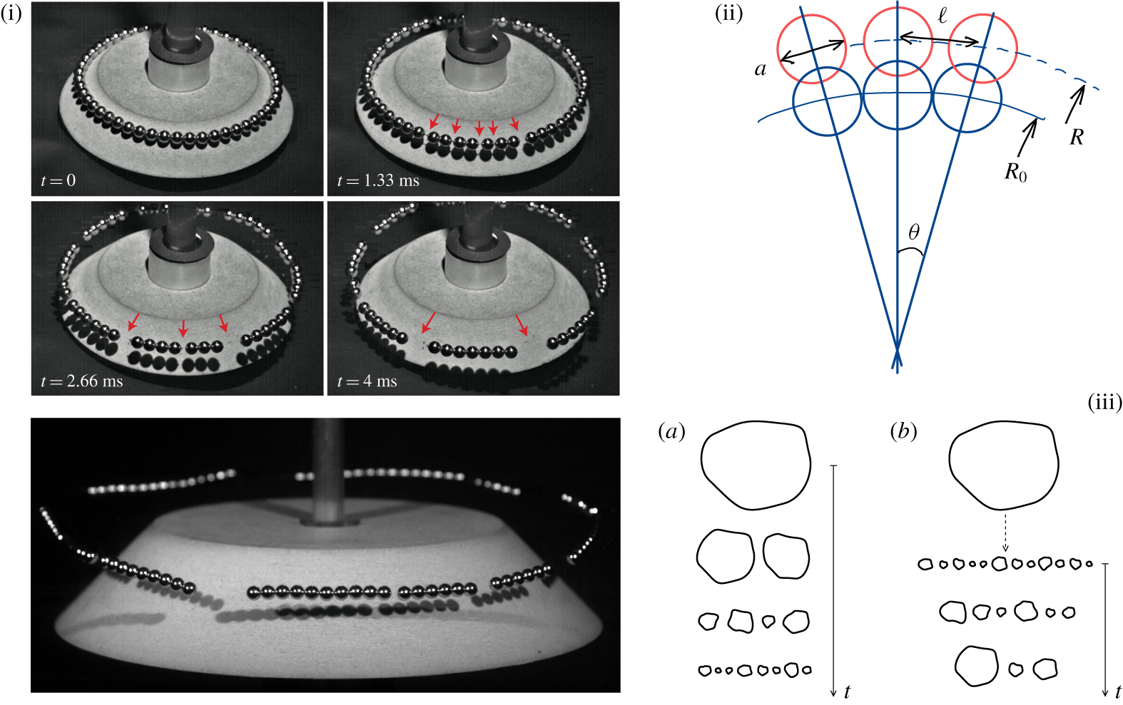
A set of spherical magnets is assembled in a necklace positioned on a cone with an incline at 45^°. The cone, guided by an axle, is released from rest at a given height and when it hits the ground, it is suddenly stopped. An initial impulse in the radial direction is communicated to each sphere, and the necklace expands at radial speed $V$. Consequently, the spheres separate from each other; the necklace is literally ‘atomized’. But, because of the attractive force linking them, the spheres start concomitantly to aggregate in bigger clusters, a process going on at an ever slowing down pace to finally stop when the clusters are too heavy, and distant from each other to aggregate. Fragments of various sizes are then irreversibly formed (the collision between clusters is inelastic, with virtually no rebound, see Hinch & Saint-Jean (Reference Hinch and Saint-Jean1999) for the opposite situation). The sequence of events, with the corresponding inverse cascade of aggregations is illustrated in figure 3.

Figure 3.

Fragmentation of a necklace of spherical magnets (Vledouts et al. Reference Vledouts, Vandenberghe and Villermaux2015, Reference Vledouts, Vandenberghe and Villermaux2016b). (i) A ring made of spherical magnets of diameter $a=5~\text{mm}$, mass $m=0.5~\text{g}$ and mutual contact force $\unicode[STIX]{x1D719}(a)$ is placed on a cone, which is let fall on the ground. At impact, each sphere is communicated a radial speed $V$ and the ring expands. The spheres separate from each other and start to aggregate, driven by the attractive magnetic force. The arrows indicate intervals between fragments. (ii) Sketch of the separation process. (iiia) The conventional direct, sequential cascade of breakups for which the arrow of time points towards ever smaller fragment sizes. (b) The inverse cascade of aggregations, occurring after the smallest sizes accessible by the system have been formed in a first step (dotted arrow). Fragment sizes get larger as time proceeds.

2.3.1 Radial deceleration

The central force between two spherical particles of diameter $a$, of magnetization density $M$ separated by a centre-to-centre distance $\ell$ is

(2.2)$$\begin{eqnarray}\unicode[STIX]{x1D719}(\ell )=\unicode[STIX]{x1D719}(a)\times \left(\frac{a}{\ell }\right)^{4},\end{eqnarray}$$

with $\unicode[STIX]{x1D719}(a)=\unicode[STIX]{x03C0}\unicode[STIX]{x1D707}_{0}M^{2}a^{2}/24$ where $\unicode[STIX]{x1D707}_{0}$ is the vacuum permeability (Jackson Reference Jackson1998). Spheres are essentially attracted by their nearest neighbours, and the first consequence of this triplet interactions along the curved necklace shape is the decrease of the expansion radial speed. Attractive forces on a curved substrate induce a Laplace, surface tension force decelerating the cohesive necklace. If $R$ is the necklace radius and $R(t=0)=R_{0}$, its equation of motion writes

(2.3)$$\begin{eqnarray}\displaystyle & \displaystyle m\ddot{R}=-\unicode[STIX]{x1D719}(R\unicode[STIX]{x1D703})\times 2\sin (\unicode[STIX]{x1D703}/2), & \displaystyle\end{eqnarray}$$

(2.4)$$\begin{eqnarray}\displaystyle & \unicode[STIX]{x1D703}=a/R_{0}\ll 1, & \displaystyle\end{eqnarray}$$

where $m$ is the sphere mass, integrating into

(2.5)$$\begin{eqnarray}{\dot{R}}^{2}=V^{2}-V_{c}^{2}\left(1-\left(\frac{R_{0}}{R}\right)^{3}\right),\quad \text{with}~V_{c}^{2}=\frac{2}{3}\frac{a\unicode[STIX]{x1D719}(a)}{m}.\end{eqnarray}$$

The critical velocity $V_{c}$ is the escape velocity of the process, meaning the velocity below which an initial expansion at velocity $V$ will coalesce back to the initial state $R_{0}$. For $V>V_{c}$, the expansion velocity ${\dot{R}}$ is strongly slowed down at short time, before reaching a steady value, smaller that $V$ as

(2.6a,b)$$\begin{eqnarray}\left(\frac{{\dot{R}}}{V}\right)^{2}\xrightarrow[{t\rightarrow 0}]{}1-\frac{V_{c}^{2}}{V}\frac{t}{R_{0}},\quad \text{and}\quad {\dot{R}}^{2}\xrightarrow[{R\rightarrow \infty }]{}V^{2}-V_{c}^{2}.\end{eqnarray}$$

This decay and final shift from $V$ reflects the transfer of kinetic energy into potential energy, the one which was spent at breaking the liaisons between the spheres. We will come back to these energetic considerations in § 11.

2.3.2 Ortho-radial aggregation

The other consequence of the central force $\unicode[STIX]{x1D719}(\ell )$ besides expansion slowing down is the concomitant aggregation of the spheres, and then of clusters of spheres. Two neighbour fragments with $p$ and $q$ spheres, respectively, separated by a distance $\ell$ between the centre of their facing end spheres interact through $\unicode[STIX]{x1D719}(\ell )$, the force between the end spheres. The equation of motion for $\ell$ then reads

(2.7)$$\begin{eqnarray}\ddot{\ell }=-\frac{\unicode[STIX]{x1D719}(a)}{m}\left(\frac{a}{\ell }\right)^{4}\left(\frac{1}{p}+\frac{1}{q}\right),\end{eqnarray}$$

whose first integral is again

(2.8)$$\begin{eqnarray}\dot{\ell }^{2}=u_{p,q}^{2}-\frac{p+q}{pq}V_{c}^{2}\left(1-\left(\frac{a}{\ell }\right)^{3}\right),\quad \text{with}~u_{p,q}=V\frac{a}{R_{0}}\frac{p+q}{2},\end{eqnarray}$$

where $u_{p,q}$ is the geometrical initial divergence velocity (i.e. in the ortho-radial direction) of two clusters of size $p$ and $q$. Making $\unicode[STIX]{x1D701}=\ell /a$ and $\unicode[STIX]{x1D70F}=u_{p,q}t/a$, we have

(2.9)$$\begin{eqnarray}\frac{\text{d}^{2}\unicode[STIX]{x1D701}}{\text{d}\unicode[STIX]{x1D70F}^{2}}=-\frac{3}{2}\frac{\unicode[STIX]{x1D716}_{p,q}}{\unicode[STIX]{x1D701}^{4}},\end{eqnarray}$$

with $\unicode[STIX]{x1D701}(0)=\dot{\unicode[STIX]{x1D701}}(0)=1$ and

(2.10)$$\begin{eqnarray}\unicode[STIX]{x1D716}_{p,q}=\left(\frac{u_{c}}{u_{p,q}}\right)^{2},\quad \text{with}~u_{c}^{2}=V_{c}^{2}\frac{p+q}{pq}.\end{eqnarray}$$

The critical velocity $u_{c}$ is the divergence velocity above which two cohesive fragments with sizes $p$ and $q$ will not reconnect. Initially, $p=q=1$ and successive cluster–cluster coalescences increase these numbers. Aggregation thus proceeds as long as $u_{p,q}<u_{c}$, or $\unicode[STIX]{x1D716}_{p,q}>1$, and the necklace fragmentation is completed as soon as $\unicode[STIX]{x1D716}_{p,q}<1$ for all neighbouring fragments of size $p$ and $q$. The fragment trajectories described by (2.9), the cluster coalescence time scales, the mean fragment growth and the details of the aggregation cascade are discussed by Vledouts et al. (Reference Vledouts, Vandenberghe and Villermaux2015); the role of pre-existing defects along the necklace is considered in Vledouts et al. (Reference Vledouts, Vandenberghe and Villermaux2016b).

2.3.3 The Weber number

In this necklace shattering example, as in all fragmentation problems, disgregation and cohesion compete and cooperate in building the overall fragment size distribution.

There is a number which measures the initial ratio of these two ingredients, namely the Weber number (it was, actually, introduced by Weber (Reference Weber1931) not even in the form of a dimensionless quantity, and in the very different context, examined in § 8, of jet stability, see also § A.5). In our example, fragmentation is completed at the end of the inverse coalescence cascade marked by $\unicode[STIX]{x1D716}_{p,q}=1$, a condition we will first write for the average fragment size $p=q=\langle n\rangle$, leaving the discussion about the distributions of fragment sizes to § 9. From (2.10), we see that

(2.11)$$\begin{eqnarray}\langle n\rangle ^{3/2}\sim \frac{V_{c}}{V}\frac{R_{0}}{a}.\end{eqnarray}$$

The surface tension $\unicode[STIX]{x1D70E}$ of the necklace is approximately such that $a^{2}\unicode[STIX]{x1D70E}\approx \int _{a}^{\infty }\unicode[STIX]{x1D719}(\ell )\,\text{d}\ell$ for this one-dimensional cohesive object so that $\unicode[STIX]{x1D70E}\approx \unicode[STIX]{x1D719}(a)/a$, and the mass of a sphere with density $\unicode[STIX]{x1D70C}$ is $m\sim \unicode[STIX]{x1D70C}a^{3}$. Introducing the particle Weber number

(2.12)$$\begin{eqnarray}We=\frac{\unicode[STIX]{x1D70C}u_{1,1}^{2}a}{\unicode[STIX]{x1D70E}},\end{eqnarray}$$

where $u_{1,1}=Va/R_{0}$ is the divergence velocity at the scale of the elementary molecule, or particle constitutive of the cohesive necklace, we can re-write (2.11) in terms of $We$ as

(2.13)$$\begin{eqnarray}\langle n\rangle \sim We^{-1/3}.\end{eqnarray}$$

This scaling relationship, in which $We$ can at most be equal to 1 for $\langle n\rangle \gtrsim 1$ can also be viewed as a simple (but flawed, see § 11) energy balance in which the kinetic energy $\frac{1}{2}\unicode[STIX]{x1D70C}\langle n\rangle a^{3}u_{\langle n\rangle ,\langle n\rangle }^{2}$ of the diverging motion $u_{\langle n\rangle ,\langle n\rangle }=\langle n\rangle u_{1,1}$ equilibrates the cohesion energy $a\unicode[STIX]{x1D719}(a)=a\unicode[STIX]{x1D70E}$. It was derived essentially in this form, and from the above reasoning, in different but related contexts (Grady Reference Grady1982, Reference Grady2006; Bazant & Caner Reference Bazant and Caner2013).

The relation (2.13) involves naturally the divergence velocity at the scale $a$ of the molecule and at that scale, $We<1$ when the necklace is not trivially atomized into single particles with $\langle n\rangle =1$. It is nevertheless customary in many applications to construct the Weber number on the sample length scale $R_{0}$, and on the injection, directly controllable velocity $V$ (Lefebvre Reference Lefebvre1989; Bayvel & Orzechowski Reference Bayvel and Orzechowski1993; Ashgriz Reference Ashgriz2011). This large-scale Weber number $\unicode[STIX]{x1D70C}V^{2}R_{0}/\unicode[STIX]{x1D70E}$ is typically very large indeed since

(2.14)$$\begin{eqnarray}We=\frac{\unicode[STIX]{x1D70C}V^{2}R_{0}}{\unicode[STIX]{x1D70E}}\left(\frac{a}{R_{0}}\right)^{3},\end{eqnarray}$$

with $a/R_{0}\ll 1$ in a macroscopic sample. Even if we will mostly use the (de facto much larger than unity) macroscopic Weber number in the sequel, one has to remember that it is the one in (2.12) which is dynamically relevant regarding fragmentation (see in particular § 11 about energetics).

2.4 Outline

We are now equipped with the essential concepts to apprehend fragmentation phenomena. After recalling classical results concerning static and dynamic equilibria in § 3, we will consider the fragmentation of liquid sheets and films in § 4, the case of shells in § 5, the specific aspects associated with a shear with a gas phase in § 6 and those with impacts in § 7. The spontaneous fragmentation of jets and threads will be discussed in § 8 and the important case of corrugated ligaments will be shown to be the key to understand drops size distributions in § 9. Direct cascades and the formation of fines will be illustrated in § 10 before we end by considerations on the energetics of fragmentation in § 11. Appendix A is a catalogue of instabilities relevant to the discussion.

3.1 Shapes of liquid volumes at rest: bubbles, films, minimal surfaces, puddles, menisci, capillary ascent, capillary length

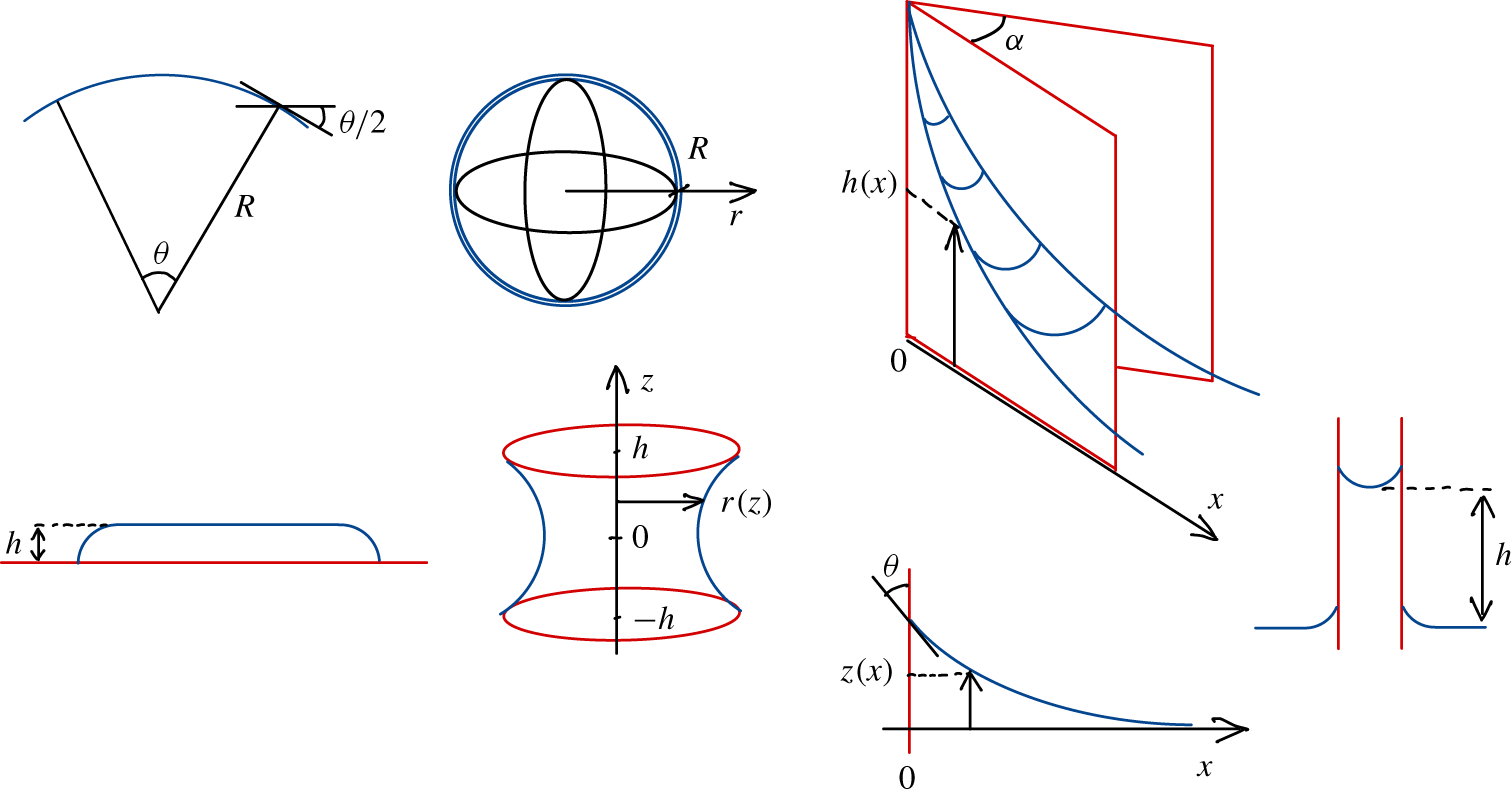
The shapes discussed below are all reported in figure 4.

Figure 4.

Classical static shapes discussed in § 3.1. From left to right and top to bottom: the Segner representation of surface tension; a spherical liquid shell of radius $R$; ascent in a wedge; a puddle lying on a solid floor; a liquid film stretched between two opened rings separated by $h$; a menisci at a solid wall (wetting angle $\unicode[STIX]{x1D703}$); capillary ascent in a tube.

3.1.1 Segner (1751) surface tension

The energy per unit surface $\unicode[STIX]{x1D70E}$ is also a force per unit length, hence the name surface tension since $\unicode[STIX]{x1D70E}\,\text{d}\boldsymbol{s}$ is the force acting tangent to the interface perpendicular to the arc length $\text{d}\boldsymbol{s}$ as first suggested by Segner in 1751 (cited by Maxwell (Reference Maxwell1875), see also Pomeau & Villermaux (Reference Pomeau and Villermaux2006)). From there, the structure of the Laplace law in (3.3) is readily recovered since, in two dimensions like in our necklace example in § 2.3, the pressure force $pR\unicode[STIX]{x1D703}$ acting on an interface arc length $R\unicode[STIX]{x1D703}$ is equilibrated by the projection of the surface tension force $2\unicode[STIX]{x1D70E}\sin (\unicode[STIX]{x1D703}/2)$ perpendicular to the interface, leading to

(3.4)$$\begin{eqnarray}p=\frac{\unicode[STIX]{x1D70E}}{R}.\end{eqnarray}$$

3.1.2 Bubble

Similarly, the surface energy $E$ of a spherical soap bubble can also be computed from the work spent by the pressure force $p(r)=4\unicode[STIX]{x1D70E}/r$ (since in (3.3) $R_{1}=R_{2}=r$ if $r$ is the current bubble radius, and the bubble shell is bounded by two sides) while inflating it up to its final radius $R$ as

(3.5)$$\begin{eqnarray}\displaystyle E & = & \displaystyle \int _{0}^{R}4\unicode[STIX]{x03C0}r^{2}p(r)\,\text{d}r\end{eqnarray}$$

(3.6)$$\begin{eqnarray}\displaystyle & = & \displaystyle 2\times 4\unicode[STIX]{x03C0}R^{2}\unicode[STIX]{x1D70E}\quad \text{(two sides)}.\end{eqnarray}$$

A soap bubble is an example of liquid shells whose fragmentation modes will be studied in § 5. Under gravity, their structure is constantly evolving, large bubbles are not even spheres, but the spheroidal shape is a good approximation for centimetric bubbles and the reason is that this shape minimizes the surface area (and therefore the surface energy) for a given volume (see the isoperimetric problem in Courant, Robbins & Stewart (Reference Courant, Robbins and Stewart1996), chapter VII, § 8 for a simple geometrical justification). It is a nice realization of the principle of least action (see e.g. Isenberg (Reference Isenberg1978) for a straightforward application to axisymmetric shapes).

3.1.3 Minimal surface

The catenoid obtained by stretching a film between two circular rings is another celebrated example of an optimal surface. The rings are opened (hence $p=0$), their radius is $R$ and they are separated by a distance $2h$. The radius of the film along the axis of revolution $z$ is $r(z)$ and $r^{\prime }=\text{d}r/\text{d}z$. The surface energy $E$ and its variation $\unicode[STIX]{x1D6FF}E$ upon modulations $\unicode[STIX]{x1D6FF}r$ from the sought optimal shape are

(3.7)$$\begin{eqnarray}\displaystyle & \displaystyle E=2\unicode[STIX]{x1D70E}\int _{-h}^{h}f(r,r^{\prime })\,\text{d}z,\quad \text{with}~f(r,r^{\prime })=2\unicode[STIX]{x03C0}r\sqrt{1+r^{\prime 2}} & \displaystyle\end{eqnarray}$$

(3.8)$$\begin{eqnarray}\displaystyle & \displaystyle \unicode[STIX]{x1D6FF}E=2\unicode[STIX]{x1D70E}\int _{-h}^{h}\left\{\frac{\unicode[STIX]{x2202}f}{\unicode[STIX]{x2202}r}-\frac{\text{d}}{\text{d}z}\frac{\unicode[STIX]{x2202}f}{\unicode[STIX]{x2202}r^{\prime }}\right\}\unicode[STIX]{x1D6FF}r\,\text{d}z. & \displaystyle\end{eqnarray}$$

The optimal shape corresponds to $\unicode[STIX]{x1D6FF}E=0$ whatever $\unicode[STIX]{x1D6FF}r$, a condition which cancels the integrand in (3.8), thus providing the Euler–Lagrange equation whose solution is the film shape

(3.9a,b)$$\begin{eqnarray}\frac{r(z)}{r_{m}}=\cosh \left(\frac{z}{r_{m}}\right),\quad \text{and}\quad \frac{R}{r_{m}}=\cosh \left(\frac{h}{r_{m}}\right)\end{eqnarray}$$

a solution (in fact a couple of solutions with one having a lower surface energy), which does exist as long as $h/R\lesssim 0.66$ for $h/r_{m}\approx 1.2$. The net curvature of the catenoid is indeed zero (Plateau Reference Plateau1873), and Delaunay (Reference Delaunay1841) has generalized this result to any non-zero constant curvature (like if the sections of the end rims were closed, and the film were either inflated, or deflated with $p\neq 0$).

3.1.4 Puddle, meniscus

A circular liquid puddle (radius $R$) lying on a flat horizontal solid surface is another illustration of the energetic cost associated with interface creation: we assume for simplicity that the liquid is indifferent to the solid, meaning that it has no tendency to wet it, or to be repelled by it (the complete problem involves a wetting angle, first introduced by Young (Reference Young1805), taken here as equal to $\unicode[STIX]{x03C0}/2$; the subtleties of wetting phenomena are very well discussed in de Gennes (Reference de Gennes1985), for example). Two kinds of energies compete, the potential energy $\unicode[STIX]{x03C0}R^{2}\int _{0}^{h}\unicode[STIX]{x1D70C}gz\,\text{d}z$ of the liquid in the gravitation field if $h$ is the puddle height, and the surface energy $\unicode[STIX]{x03C0}R^{2}\unicode[STIX]{x1D70E}$. For a given puddle volume $\unicode[STIX]{x1D6FA}=\unicode[STIX]{x03C0}R^{2}h$, the puddle height $h$ makes the net energy $E$

(3.10)$$\begin{eqnarray}\frac{E}{\unicode[STIX]{x1D6FA}}=\frac{1}{2}\unicode[STIX]{x1D70C}gh+\frac{\unicode[STIX]{x1D70E}}{h}\end{eqnarray}$$

minimum ($\unicode[STIX]{x2202}E/\unicode[STIX]{x2202}h=0$, $\unicode[STIX]{x2202}^{2}E/\unicode[STIX]{x2202}h^{2}>0$), when

(3.11)$$\begin{eqnarray}h=\sqrt{\frac{2\unicode[STIX]{x1D70E}}{\unicode[STIX]{x1D70C}g}}\equiv a,\end{eqnarray}$$

where $a$ is called the capillary length scale (Landau & Lifshitz Reference Landau and Lifshitz1987). It is, for the same reason, this length scale which sets the typical dimensions of the liquid meniscus wetting a vertical solid wall at an angle $\unicode[STIX]{x1D703}$. The expression of the meniscus profile $z(x)$ is complicated (see e.g. Landau & Lifshitz (Reference Landau and Lifshitz1987) and de Gennes, Brochard-Wyart & Quere (Reference de Gennes, Brochard-Wyart and Quere2004)), but the maximal elevation of the meniscus above the flat interface level far from it ($x\gg a$) is given by $h=a\sqrt{1-\sin \unicode[STIX]{x1D703}}$ while, when $\unicode[STIX]{x1D703}\lesssim \unicode[STIX]{x03C0}/2$, one has $z(x)\approx h\text{e}^{-x/a}$; the meniscus is localized indeed.

3.1.5 Capillary ascents

Menisci are one example of the famous shapes, which had remained paradoxical before he rationalized them, solved by Laplace. Others are the ascent of a wetting liquid in the sharp interstice between two plates forming a dihedral (Taylor Reference Taylor1712; Bouasse Reference Bouasse1924; Higuera, Medina & Liñán Reference Higuera, Medina and Liñán2008), whose profile is $z(x)\sim a^{2}/(\unicode[STIX]{x1D6FC}x)$ with $\unicode[STIX]{x1D6FC}$ the angle of the dihedral, and $x$ the distance from its apex, and of course the celebrated capillary ascent in a narrow tube: the weight of the liquid column $\unicode[STIX]{x1D70C}gh\unicode[STIX]{x03C0}r^{2}$ is balanced by the capillary force $2\unicode[STIX]{x03C0}r\unicode[STIX]{x1D70E}\cos \unicode[STIX]{x1D703}$ at the capillary circumference, if $r$ is its radius, and $\unicode[STIX]{x1D703}$ the wetting angle. The liquid elevation is given by Jurin’s law (Jurin (Reference Jurin1719), who quantified the inverse relationship $h\sim r^{-1}$)

(3.12)$$\begin{eqnarray}\frac{h}{a}=\frac{a}{r}\cos \unicode[STIX]{x1D703}\end{eqnarray}$$

and is equal to zero when the liquid is indifferent to the solid (i.e. $\unicode[STIX]{x1D703}=\unicode[STIX]{x03C0}/2$ like for water on a surface of silanized glass).

3.2 Dynamic equilibria: film edge recession, Taylor–Culick formulae, paradox, holes, Savart sheets and bells

Equilibrium does not mean absence of motion. Capillary forces may be balanced by inertial and viscous forces, as in the situations we describe below.

3.2.1 Rim recession: straight edges

Liquid sheets extruded through slits are bordered by a rim, which has its own dynamics. Holes may nucleate in liquid films, sheets or shells (see § 4), and open spontaneously. The reason is that at the edge of a ruptured film, surface tension forces are no more balanced, and communicate inertia to the liquid. We discuss below the nature of this transfer, its sensitivity to the liquid properties, geometry (planar or circular), starting first by the integral formulation of Taylor (Reference Taylor1959c).

A film of uniform thickness $h$ and surface tension $\unicode[STIX]{x1D70E}$ is bounded by a free straight edge with velocity $v={\dot{x}}$. As the edge recedes under the action of capillary traction, it accumulates a mass $m$ initially constitutive of the undisturbed film, in a region of size $L$, which is the typical distance from the edge where fluid particles are accelerated irreversibly from $v=0$ (the film is at rest), to $v$. This region defines the extent of the sheet rim. The force, and mass balances (per unit rim length) over this region write

(3.13a,b)$$\begin{eqnarray}{\dot{P}}=2\unicode[STIX]{x1D70E},\quad \text{and}\quad {\dot{m}}=\unicode[STIX]{x1D70C}hv,\end{eqnarray}$$

where $P=mv$ is the rim momentum. The factor 2 stands for the two sides of the film. Expanding the first relation in (3.13) as $m\dot{v}+v{\dot{m}}=2\unicode[STIX]{x1D70E}$ we seek a constant receding velocity (as suggested by experiments, see Ranz (Reference Ranz1959), Koros, Deckers & Boudart (Reference Koros, Deckers and Boudart1960), Frankel & Mysels (Reference Frankel and Mysels1969), McEntee & Mysels (Reference McEntee and Mysels1969a) and Pandit & Davidson (Reference Pandit and Davidson1990)), leading to

(3.14)$$\begin{eqnarray}v=\sqrt{\frac{2\unicode[STIX]{x1D70E}}{\unicode[STIX]{x1D70C}h}},\end{eqnarray}$$

called the Taylor–Culick velocity. It was established along the above lines by Taylor (Reference Taylor1959c) in the context of freely expanding liquid sheets and independently, in the circular geometry suitable to holes opening on a soap film, by Culick (Reference Culick1960), himself inspired by experiments of Ranz (Reference Ranz1959). Equations (3.13) can be written

(3.15)$$\begin{eqnarray}\frac{\text{d}}{\text{d}t}\left(v\int _{0}^{t}\unicode[STIX]{x1D70C}hv\,\text{d}t\right)=2\unicode[STIX]{x1D70E},\end{eqnarray}$$

which, for a film with constant thickness indeed leads to $x\,{\dot{x}}=v^{2}t$, or $x=vt$ when $m(0)=0$. The velocity is constant, given by (3.14), from the start. Although the pulling force $2\unicode[STIX]{x1D70E}$ is permanent, it is the rim velocity which is constant, and not its acceleration, because the mass $m$ is itself increasing on the way. The cases of an initial non-uniform film profile $h(x)$ was considered by Keller, King & Ting (Reference Keller, King and Ting1995) and Raufaste et al. (Reference Raufaste, Celestini, Barzyk and Frisch2015), and non-zero mass by Lhuissier & Villermaux (Reference Lhuissier and Villermaux2011).

Culick offered a deeper understanding of (3.14) in correcting a notable, but interesting mistake by Dupré (Reference Dupré1867, Reference Dupré1869), echoed in plain words by Lord Rayleigh (1891). The model of Dupré consisted in attributing the entire surface energy consumed when the rim has travelled a distance $x$ to the kinetic energy of the rim mass $m=\unicode[STIX]{x1D70C}hx$, that is $\frac{1}{2}mv^{2}\neq 2\unicode[STIX]{x1D70E}x$, a flawed equality leading to an over-estimated velocity $\sqrt{2}v$ when $v$ is given by the (correct) value in (3.14). The reason why this ‘sentimental’ energy balance (on which we come back in § 11) fails is that it disregards the energy sink of the inelastic process of accelerating the fluid in the undisturbed film up to the velocity of the edge, a fraction of the available energy dissipated by internal viscous fluid friction which represents exactly half the consumed surface energy. Equivalently, this sink represents the energy loss at a sudden expansion when the fluid particles pass from the film to the thicker rim (see § 11).

Estimating the viscous dissipation rate $\int \unicode[STIX]{x1D702}(\unicode[STIX]{x1D735}\boldsymbol{v})^{2}\,\text{d}\unicode[STIX]{x1D6FA}$ by $\unicode[STIX]{x1D702}(v/\unicode[STIX]{x1D6FF})^{2}\unicode[STIX]{x1D6FA}$ for a dissipation volume $\unicode[STIX]{x1D6FA}\approx h\ell \unicode[STIX]{x1D6FF}$ and equating it to the rate of energy loss $\frac{1}{2}(2\unicode[STIX]{x1D70E}\ell v)$ along a rim portion length $\ell$, Culick (Reference Culick1960) further computed the dissipation length scale $\unicode[STIX]{x1D6FF}$ as

(3.16)$$\begin{eqnarray}\displaystyle \frac{\unicode[STIX]{x1D6FF}}{h} & {\sim} & \displaystyle \frac{\unicode[STIX]{x1D702}v}{\unicode[STIX]{x1D70E}}\end{eqnarray}$$

(3.17)$$\begin{eqnarray}\displaystyle & {\sim} & \displaystyle \frac{\unicode[STIX]{x1D702}}{\sqrt{\unicode[STIX]{x1D70C}h\unicode[STIX]{x1D70E}}}\equiv Oh,\end{eqnarray}$$

thus defining the Ohnesorge number $Oh$.

Figure 5.

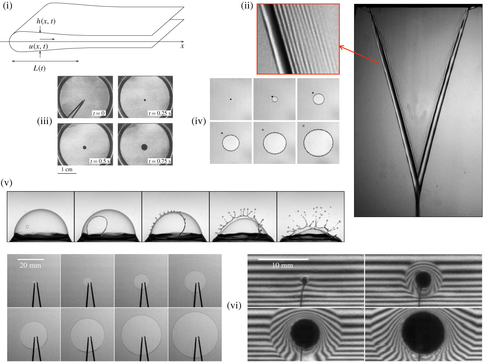
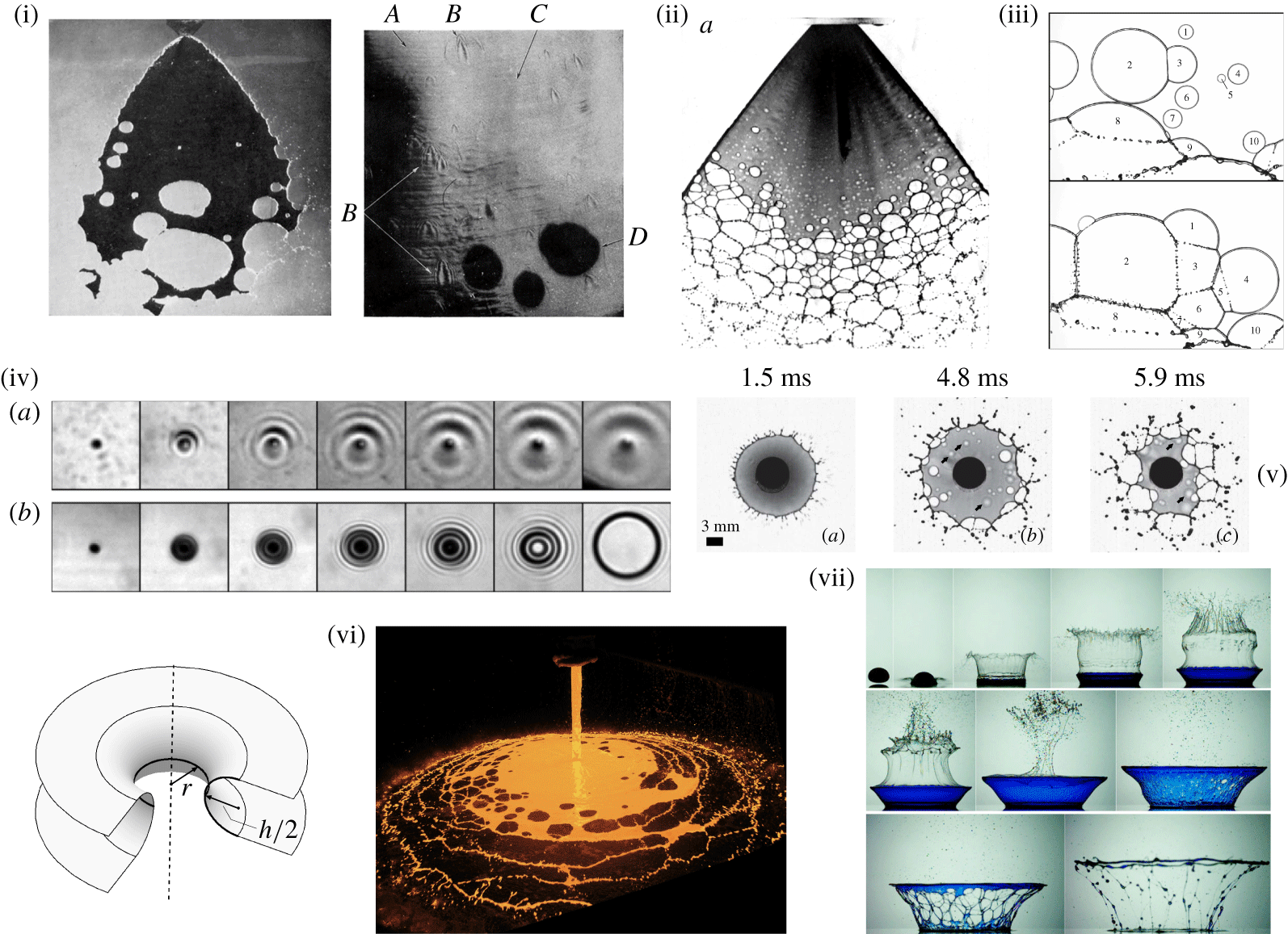
Bounded liquid sheets: rim recession and hole opening. (i) Sketch of a receding rim. (ii) A liquid sheet formed from a slit with edges receding at the constant Taylor–Culick velocity. Short capillary waves propagate ahead from the front. (iii) Hole expansion on a viscous film (Debrégeas, Martin & Brochard-Wyart Reference Debrégeas, Martin and Brochard-Wyart1995). (iv) Hole expansion on a water film. (v) Hole expansion on a surface bubble (Lhuissier & Villermaux Reference Lhuissier and Villermaux2012a). (vi) Hole expansion on a soap film seen in transparency (left) and in interferometry, highlighting the characteristic ‘aureole’ (Lhuissier & Villermaux Reference Lhuissier and Villermaux2009a).

The problem of a receding rim is thus one of the rare instances in Fluid Mechanics where the net amount of dissipation can be computed exactly from first principles, even in the presence of inertia. Like in turbulent flows, the dissipative scale self-adapts to make the energy dissipation finite and independent of the fluid viscosity $\unicode[STIX]{x1D702}$ (thus including when $\unicode[STIX]{x1D702}\rightarrow 0$). It is, in this respect, the analogue of Taylor’s microscale (Taylor (Reference Taylor1935), or Liepmann–Taylor scale if one likes to view it as the thickness of internal shear layers (Dimotakis Reference Dimotakis2000)) in turbulent flows obtained by equating the viscous dissipation rate per unit mass $\unicode[STIX]{x1D708}(u/\unicode[STIX]{x1D6FF})^{2}$ with the – viscosity independent – kinetic energy injection rate $u^{2}/(L/u)$ with $L$ and $u$ the stirring scale and velocity, respectively, leading to the familiar relation $\unicode[STIX]{x1D6FF}/L\sim Re^{-1/2}$ if $Re=uL/\unicode[STIX]{x1D708}$ is the Reynolds number based on the kinematic viscosity $\unicode[STIX]{x1D708}$ of the fluid. The end of the ‘cascade’ towards smaller scales where now $u(\unicode[STIX]{x1D6FF})\sim u(\unicode[STIX]{x1D6FF}/L)^{1/3}$ is marked by the Kolmogorov scale $\unicode[STIX]{x1D6FF}/L\sim Re^{-3/4}$ (Kolmogorov Reference Kolmogorov1941a). Like in the rim problem, $\unicode[STIX]{x1D6FF}\rightarrow 0$ when $\unicode[STIX]{x1D702}\rightarrow 0$ while the energy dissipation rate remains finite.

Viscosity does impact this problem, however, through a not yet alluded to quantity, namely the rim extent $L$. We just saw that the dissipation scale $\unicode[STIX]{x1D6FF}$ in (3.17) adapts to fulfil the mass and momentum constraints in (3.13). The rim extent follows a qualitatively similar trend. For $Oh\ll 1$, the liquid collects in a rim with a close-to-circular cross-section with radius $L\sim h[1+(vt/h)^{2}]^{1/4}\rightarrow \sqrt{vht}$ given by mass conservation (see e.g. Gordillo et al. Reference Gordillo, Agbaglah, Duchemin and Josserand2011) and where recirculation motions dissipate the necessary amount of energy at a scale $\unicode[STIX]{x1D6FF}\ll L$.

For $Oh\gg 1$, however, the picture is different. There is no collecting rim anymore, because $\unicode[STIX]{x1D6FF}$ is larger than $h$ from the start. Dissipation is spread out diffusively along the – essentially flat – film which is now set into motion by longitudinal viscous stresses. Savva & Bush (Reference Savva and Bush2009) have shown that in this limit, a fair, short time, slender slope ($h^{\prime }\ll 1$) description of the velocity $u(x,t)$ along the film (with ${\dot{x}}_{0}=u(x_{0},t)$ the film edge velocity) is given by

(3.18)$$\begin{eqnarray}\unicode[STIX]{x2202}_{t}u=4\unicode[STIX]{x1D708}\unicode[STIX]{x2202}_{x}^{2}u+v^{2}\unicode[STIX]{x1D6FF}(x-x_{0}),\end{eqnarray}$$

valid for $x>h$. The film curvature $\unicode[STIX]{x1D705}$ is of order $h^{-1}$ for distances to the edge of order $h$ and essentially zero elsewhere, so that its spatial variation at the edge location $x_{0}$ is caricatured as a Dirac Delta, that is $\unicode[STIX]{x2202}_{x}\unicode[STIX]{x1D705}\approx (2/h)\unicode[STIX]{x1D6FF}(x-x_{0})$. The velocity along the film is thus given by the impulse response of a diffusion equation, providing

(3.19a,b)$$\begin{eqnarray}\displaystyle & \displaystyle {\dot{x}}_{0}\sim v\sqrt{\frac{t}{\unicode[STIX]{x1D70F}_{vis}}},\quad \text{and}\quad L\sim h\left(\frac{t}{\unicode[STIX]{x1D70F}_{vis}}\right)^{3/2}, & \displaystyle\end{eqnarray}$$

(3.20)$$\begin{eqnarray}\displaystyle & \displaystyle \text{where}~\unicode[STIX]{x1D70F}_{vis}=\frac{\unicode[STIX]{x1D702}h}{2\unicode[STIX]{x1D70E}}\equiv \frac{\unicode[STIX]{x1D708}}{v^{2}}, & \displaystyle\end{eqnarray}$$

with $v$ the Taylor–Culick velocity in (3.14) above. The relaxation distance $L$ of the viscous stress from the film edge does depend on the liquid viscosity $\unicode[STIX]{x1D702}$, but this short-time behaviour is a transient, and the film edge finally relaxes towards $v$, independent of $\unicode[STIX]{x1D702}$ (see also Chepushtanova & Kliakhandler Reference Chepushtanova and Kliakhandler2007). During the transient as the edge accelerates, the global momentum balance ${\dot{P}}=2\unicode[STIX]{x1D70E}$ in (3.13) is, however, always fulfilled, provided the film momentum $P=\unicode[STIX]{x1D70C}\int hu\,\text{d}x$ is fully integrated, from the film edge in $x_{0}$ to distances far away from it, namely larger than $L$, which itself increases in time.

3.2.2 Circular geometry: holes

Liquid films and sheets may nucleate holes. We devote the entire § 4.2 to the cause of the piercing event, but we describe here the opening dynamics of the hole once it has been formed. The circular geometry offers a slight complication in the sense that the border of the film curvature presents now two contributions, of opposite sign, reading $\unicode[STIX]{x1D705}=1/h-1/r_{0}(t)$ where $r_{0}(t)$ is the hole radius. The classical study by Taylor & Michael (Reference Taylor and Michael1973) has elegantly shown that the shape of the hole envelope is analogous to the catenary discussed in § 3.1.3 and that the condition for hole opening coincides with the condition for the catenoid stability: the hole has to be large enough ($r_{0}/h>1.32$) to open spontaneously, otherwise it heals (i.e. $r_{0}(t)\rightarrow 0$ in a finite time, see Courbin & Stone (Reference Courbin and Stone2006) for an experimental illustration). The axisymmetric version of the balances in (3.13) is approximately given, in the inviscid limit for the scaled hole radius $\unicode[STIX]{x1D709}=r_{0}(t)/h$ with $t\equiv vt/h$, by

(3.21)$$\begin{eqnarray}\dot{\unicode[STIX]{x1D709}}^{2}+\frac{1}{2}\unicode[STIX]{x1D709}\ddot{\unicode[STIX]{x1D709}}=1-\frac{\unicode[STIX]{x03C0}}{4\unicode[STIX]{x1D709}},\end{eqnarray}$$

which both restores the planar limit in (3.14), that is $\dot{\unicode[STIX]{x1D709}}=1$, and describes hole healing $\unicode[STIX]{x1D709}\sim (1-t)^{2/3}$ depending on $\unicode[STIX]{x1D709}$ being much larger or smaller than $\unicode[STIX]{x03C0}/4\approx 0.78$, respectively (see also Lv, Eigenbrod & Hard (Reference Lv, Eigenbrod and Hard2018) for the healing dynamics in the presence of gravity).

The circular geometry has nevertheless a real consequence on this rim recession problem in the viscous limit. The analogue of the initial dynamics (3.18) describing now the radial velocity field $u(r,t)$ in the film for $r_{0}/h\gg 1$ is

(3.22)$$\begin{eqnarray}\unicode[STIX]{x2202}_{t}(ur)=4\unicode[STIX]{x1D708}\left(\unicode[STIX]{x2202}_{r}^{2}(ur)-\frac{\unicode[STIX]{x2202}_{r}(ur)}{r}\right)+v^{2}r_{0}\unicode[STIX]{x1D6FF}(r-r_{0})\end{eqnarray}$$

a two-dimensional diffusion equation which solves for the hole radius velocity ${\dot{r}}_{0}(t)=u(r_{0},t)$ as

(3.23)$$\begin{eqnarray}r_{0}(t)=r_{0}(0)\text{e}^{t/2\unicode[STIX]{x1D70F}_{vis}},\end{eqnarray}$$

an exponential growth in contrast to the power law found in (3.19a,b) for the planar limit (Savva & Bush Reference Savva and Bush2009). Geometry thus impacts the form of laws.

Debrégeas et al. (Reference Debrégeas, Martin and Brochard-Wyart1995), Debrégeas, de Gennes & Brochard-Wyart (Reference Debrégeas, de Gennes and Brochard-Wyart1998) have given an ‘à la Dupré’ description of this problem, by attributing the entire film surface energy consumed by the hole opening to the dissipation of energy by viscous stresses, an equality which fails quantitatively in the inertial limit as recalled above, but which is legitimate for $Oh\gg 1$ when inertia is sub-dominant. Equating the rate of viscous dissipation

(3.24)$$\begin{eqnarray}\int _{r_{0}(t)}^{\infty }2\unicode[STIX]{x03C0}rh\frac{\unicode[STIX]{x1D702}}{2}[(\unicode[STIX]{x2202}_{r}u)^{2}+(u/r)^{2}]\,\text{d}r,\end{eqnarray}$$

with $u(r,t)={\dot{r}}_{0}r_{0}/r$ to the rate of surface energy destruction $2\unicode[STIX]{x03C0}\unicode[STIX]{x1D70E}h{\dot{r}}_{0}^{2}$ over an essentially constant in thickness film actually leads to (3.23).

Equation (3.23) is the axisymmetric response to a genuine diffusive, viscous dynamics and should not, as noted by Debrégeas et al. (Reference Debrégeas, Martin and Brochard-Wyart1995), be confused with a viscoelastic effect. When the mechanical response of the material is elastic, the initial stress propagation along the film is mediated by a shock wave, a phenomenon also observed in soap films coated by a rigid layer of surfactants (McEntee & Mysels Reference McEntee and Mysels1969b; Frankel & Mysels Reference Frankel and Mysels1969) and responsible for the formation of a so-called ‘aureole’ propagating upstream from the hole edge with a dramatic consequence on its stability (see Lhuissier & Villermaux (Reference Lhuissier and Villermaux2009a) and § 6). When released, the extremity of a stretched rubber band recedes at constant velocity, proportional to the speed of sound in the material, and to a function of the initial stretch (Vermorel, Vandenberghe & Villermaux Reference Vermorel, Vandenberghe and Villermaux2007) while an isotropically stretched rubber sheet will, when ruptured at a point, more likely dissipate energy by opening radial fractures (Moulinet & Adda-Bedia Reference Moulinet and Adda-Bedia2015).

3.2.3 Savart sheet

The premonitory intuition of Savart was that by diverting promptly a liquid stream, one would gain information on the nature of the liquid itself. The configuration, declined in two memoirs (Savart Reference Savart1833c,Reference Savartd) out of four (the two others being Savart (Reference Savart1833a,Reference Savartb), all published in 1833 in the Annales de Chimie Physique), consists in letting a jet impacting normally onto a small solid disk (figure 6). It has indeed proved to be an extraordinary laboratory to study the consequence of liquid cohesion on the sensible world.

The incident momentum flux (per unity liquid density $\unicode[STIX]{x1D70C}$) carried by the jet $\unicode[STIX]{x03C0}d_{0}^{2}/4u_{0}^{2}$ is cancelled by the reaction force of the impactor, and is distributed radially in an isotropic fashion. It is, however, reduced by an amount of order $\unicode[STIX]{x03C0}d_{i}\unicode[STIX]{x1D6FF}u_{0}u$, lost in the boundary layer at the surface of the impactor (with diameter $d_{i}$). The thickness of that boundary layer is of order (Schlichting Reference Schlichting1987)

(3.25)$$\begin{eqnarray}\unicode[STIX]{x1D6FF}\sim \sqrt{\frac{\unicode[STIX]{x1D708}d_{i}}{u_{0}}}.\end{eqnarray}$$

If $\unicode[STIX]{x1D6FF}$ is usually small compared to the diameter of the impactor, it may compare with the sheet thickness itself whose inviscid value at the impactor lip is given by mass conservation

(3.26)$$\begin{eqnarray}h_{inv}=\frac{d_{0}^{2}}{8d_{i}}.\end{eqnarray}$$

It is only when the Reynolds number $Re=ud_{0}/\unicode[STIX]{x1D708}$ is much larger than unity that the ratio

(3.27)$$\begin{eqnarray}\unicode[STIX]{x1D6FD}=\frac{\unicode[STIX]{x1D6FF}}{h_{inv}}=2\sqrt{\frac{(d_{i}/d_{0})^{3}}{Re}}\end{eqnarray}$$

is appreciably small.

Figure 6.

Savart sheets and bell. (i) Axisymmetric liquid sheet states: (a) smooth regime. (b) Flapping regime for larger Weber number (higher than 1000). (c) Perturbation of the smooth regime by imposing vertical oscillations of the impact rod. (ii) Close-up views of the free rim of a smooth liquid sheet, for cases (a) and (b) above, adapted from Bremond, Clanet & Villermaux (Reference Bremond, Clanet and Villermaux2007). (iii) An instantaneous view of a viscous Savart sheet with a liquid 320 more viscous than water (the water case with the same injection parameters is shown in the insert, adapted from Villermaux, Pistre & Lhuissier (Reference Villermaux, Pistre and Lhuissier2013)). (iv) Collision at an angle (90^°) of two jets of ethanol (left) and water (right), adapted from Bremond & Villermaux (Reference Bremond and Villermaux2006). (v) A stationary Savart bell exhibiting the characteristic catenoid shape.

The step velocity across the sheet profile at the impactor lip relaxes by viscous smoothing as it leaves the impactor over a short radial distance of order $u_{0}h^{2}/\unicode[STIX]{x1D708}$ towards a uniform (shear-less) profile with velocity $u$ and thickness $h$, carrying the rest of momentum $2\unicode[STIX]{x03C0}rhu^{2}$, and the jet flow rate $\unicode[STIX]{x03C0}d_{0}^{2}/4u_{0}=2\unicode[STIX]{x03C0}rhu$, thus providing (Villermaux et al. Reference Villermaux, Pistre and Lhuissier2013)

(3.28a,b)$$\begin{eqnarray}u=\frac{u_{0}}{1+\unicode[STIX]{x1D6FD}}\quad \text{and}\quad h(r)=\frac{d_{0}^{2}}{8r}(1+\unicode[STIX]{x1D6FD}).\end{eqnarray}$$

The ratio of the impulse carried by the sheet in a given radial direction (the average over the $2\unicode[STIX]{x03C0}$ angular directions is zero for an axisymmetric sheet), to the incident impulse is thus

(3.29)$$\begin{eqnarray}\frac{\text{sheet impulsion}}{\text{incident impulsion}}\sim \frac{u^{2}hd_{i}}{u_{0}^{2}d_{0}^{2}}=\frac{1}{1+\unicode[STIX]{x1D6FD}},\end{eqnarray}$$

indeed smaller than unity. The above relations interpolate between the thin boundary layer limit ($\unicode[STIX]{x1D6FD}\ll 1$) for which $u\approx u_{0}(1-\unicode[STIX]{x1D6FD})$ and the viscous limit ($\unicode[STIX]{x1D6FD}\gg 1$) which involves corrections in $\unicode[STIX]{x1D6FD}^{2}$ (Watson Reference Watson1964).

Although the surface area of an element of volume travelling radially increases in proportion of $r/d_{0}$ (or of $d_{0}/h(r)$, equivalently), surface tension plays no role in its radial dynamics, which is purely ballistic. The reason is that the net force in the plane of the (essentially flat) sheet integrated over any closed contour

(3.30)$$\begin{eqnarray}\oint \unicode[STIX]{x1D70E}\,\text{d}\boldsymbol{s}=\mathbf{0}\end{eqnarray}$$

is exactly zero, as long as $\unicode[STIX]{x1D70E}$ is constant over the sheet, as noted by Marmottant, Villermaux & Clanet (Reference Marmottant, Villermaux and Clanet2000). In the absence of other ingredients like the interaction with the surrounding ambient medium, or heterogeneous hole nucleation processes studied in the next sections, the velocity $u$ is thus purely radial, and conserved. Cohesion only compensates for the radial divergence of the streamlines in thinning the sheet for volume conservation, but at the expense of no net work (see in this respect the historical mistake of Hagen reported literally in Bouasse (Reference Bouasse1923), § 107).

Following Taylor (Reference Taylor1959c), it is admitted that the radial expansion is halted by capillary confinement when the Taylor–Culick velocity in (3.14) equals the radial speed $u$ or, equivalently, when the momentum flux of the sheet equilibrates surface tension forces, that is

(3.31)$$\begin{eqnarray}\unicode[STIX]{x1D70C}u^{2}h(R_{TC})=2\unicode[STIX]{x1D70E}.\end{eqnarray}$$

We will see in § 4 that this is not exactly true and that the corresponding sheet radius anticipated from (3.31)

(3.32)$$\begin{eqnarray}\displaystyle & \displaystyle R_{TC}=d_{0}\frac{We}{16}\frac{1}{1+\unicode[STIX]{x1D6FD}} & \displaystyle\end{eqnarray}$$

(3.33)$$\begin{eqnarray}\displaystyle & \displaystyle \xrightarrow[{\unicode[STIX]{x1D6FD}\rightarrow 0}]{}d_{0}\frac{We}{16}\quad \text{with}~We=\frac{\unicode[STIX]{x1D70C}u_{0}^{2}d_{0}}{\unicode[STIX]{x1D70E}} & \displaystyle\end{eqnarray}$$

actually represents an upper bound. As $We$ increases by an increase of the injection velocity $u_{0}$, the Reynolds number increases as well, and hence $\unicode[STIX]{x1D6FD}$ decreases. The overall dependence of $R_{TC}$ on $We$ is thus a steeper than the one known for the inviscid case ($R_{TC}/d_{0}\sim We$), precisely because the relative momentum loss due to viscosity progressively fades away for larger $Re$. Also, viscosity delays the transition to the flapping regime to be analysed in § 6. There are two concomitant reasons for this delay: the liquid is slowed down, and the sheet is conversely thickened (3.28). For instance, the sheet thickness at the maximal smooth radial extension is

(3.34)$$\begin{eqnarray}h(R_{TC})=\frac{d_{0}}{We}(1+\unicode[STIX]{x1D6FD})^{2}.\end{eqnarray}$$

It is thus doubly difficult for the weakened shear $u$ (by a factor $1+\unicode[STIX]{x1D6FD}$, see (3.28)) to move a heavier because thicker sheet (by a factor $(1+\unicode[STIX]{x1D6FD})^{2}$) perpendicular to its plane and trigger an undulatory motion (even if the transit time has been augmented) hence the mandatory recourse to higher Weber numbers for it to be possible (see § 6).

Note finally that the same concepts apply to non-axisymmetric impacts like those made from the collision of two identical jets at an angle, forming an elongated, bay leaf kind of shape which is well represented by elementary mass and momentum balances, as long as the rim does not fragment. The global extent of the sheet, its width and length, are both proportional to $We$, like the radius of a circular sheet (Hasson & Peck Reference Hasson and Peck1964; Bremond & Villermaux Reference Bremond and Villermaux2006).

3.2.4 Savart bell

Making a perfectly flat sheet from the impact of a perpendicular jet on a solid disk is actually difficult (see the method of Clanet & Villermaux (Reference Clanet and Villermaux2002) to achieve this singular limit). The angle $\unicode[STIX]{x1D6FC}$ with which the sheet leaves the impactor may not be equal to $\unicode[STIX]{x03C0}/2$. In that case, for instance when $\unicode[STIX]{x1D6FC}<\unicode[STIX]{x03C0}/2$, the sheet bends in an axisymmetric way, forming a so-called bell, eventually closing at some downstream distance from the impact point (Savart Reference Savart1833c; Boussinesq Reference Boussinesq1869a,Reference Boussinesqb; Taylor Reference Taylor1959a). The reason for the bending is liquid cohesion, through Laplace pressure, balanced by the sheet centrifuge force. If $r(z)$ is the radius of the bell at the axial position $z$ from the impact point, the sheet presents two components of curvature, namely $R_{1}^{-1}=1/r\sqrt{1+r^{\prime 2}}$ and the other $R_{2}^{-1}=r^{\prime \prime }/(1+r^{\prime 2})^{3/2}$ in the plane containing the $z$-axis. When gravity is negligible and when the pressure difference between the inside and the outside of the bell is zero, equilibrium is described by

(3.35)$$\begin{eqnarray}\frac{\unicode[STIX]{x1D70C}u^{2}h(r)}{2\unicode[STIX]{x1D70E}}\frac{1}{R_{2}}=\frac{1}{R_{1}}+\frac{1}{R_{2}},\end{eqnarray}$$

where $u$ and $h(r)$ are both given in (3.28). Unlike for a bubble where the two radii of curvature are both equal to the bubble radius, the equilibrium above is not left unchanged by the substitution $R_{1}\leftrightarrow R_{2}$ (Clanet Reference Clanet2007). Symmetry is broken, and the bell is not spherical; it is actually a catenoid (Boussinesq Reference Boussinesq1869a,Reference Boussinesqb)

(3.36)$$\begin{eqnarray}\frac{L-r(z)}{L-r_{m}}=\cosh \left(\frac{z-z_{m}}{L-r_{m}}\right),\end{eqnarray}$$

with $z_{m}$ being the distance at which the maximal radius $r_{m}$ is reached, both functions of the initial sheet deflection $r^{\prime }(0)=\tan \unicode[STIX]{x1D6FC}$ and of the length scale $L=d_{0}We/16$ setting the overall size of the bell, which closes on the axis at $2z_{m}$. The influence of gravity, when aligned with the $z$-axis, can be quantified (Clanet Reference Clanet2007), and Lhuissier & Villermaux (Reference Lhuissier and Villermaux2012b) have studied the important case where the bell is pressurized with respect to its environment, leading to a singular, unstable shape studied in § 5.2.

4.1 Phenomena at the rim: cusps

The main shortcoming of Taylor’s representation in (3.31) is that it is solely grounded on momentum equilibrium, disregarding the fate of the liquid accumulating in the rim. Another flaw is that in nature, the rims bordering liquid sheets do not remain straight for long, and soon present a series of indentations, particularly obvious on the steady state configuration of the Savart sheet.

In reality, the liquid does not accumulate in the rim, and is always removed in some way; there are plenty of mechanisms serving this purpose: by gravity dripping from stationary rims as those found in Savart sheets (Clanet & Villermaux Reference Clanet and Villermaux2002; Villermaux et al. Reference Villermaux, Pistre and Lhuissier2013), by centripetal forces when the liquid flows along a curved rim (Bush & Hasha Reference Bush and Hasha2004; Bremond & Villermaux Reference Bremond and Villermaux2006) or when the rim trajectory is curved like in spinning cups or bursting bubbles (Eisenklam Reference Eisenklam1964; Lhuissier & Villermaux Reference Lhuissier and Villermaux2012a), by non-Galilean body forces when the rim is decelerated (Villermaux & Bossa Reference Villermaux and Bossa2011), by an electric field for charged liquids (Rozhkov, Prunet-Foch & Vignes-Adler Reference Rozhkov, Prunet-Foch and Vignes-Adler2015; Brosseau & Vlahovska Reference Brosseau and Vlahovska2017) etc. … In all cases, the liquid is torn off from the rim at a length scale prescribed by a corresponding instability, thus altering its straight shape, which gets distorted.

de Gennes (Reference de Gennes1996) had a very clever proposal to solve the Dupré–Rayleigh paradox recalled in § 3.2.1, by offering a non-dissipative solution to the rim recession problem, involving droplet ejection from the rim, at 45^° out of the sheet plane. In that vision, both mass and momentum are conserved (as well as kinetic energy), with no mass accumulation by the rim. de Gennes was not truthfully convinced by his scenario which indeed proved to be incorrect (he writes: ‘Up to now, as far as I know, nobody has seen droplets escaping during film rupture!’ which is also incorrect, but for other reasons discussed in § 6), a scenario which has nevertheless the right flavour of the true scenario.

Figure 7.

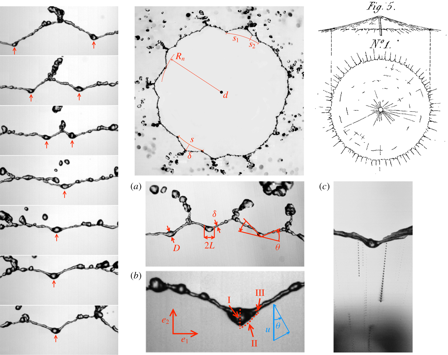
Cusps at the border of Savart sheets: shape and dynamics. Instantaneous views from above and a comparison with Savart’s drawings, made by eye. There are in the mean of the order of $N\approx 10$ cusps around the sheet, at the tip of which droplets are formed. Their mean shape is well defined, but they also nucleate, coalesce as they move along the sheet (adapted from Gordillo, Lhuissier & Villermaux (Reference Gordillo, Lhuissier and Villermaux2014) and Villermaux & Almarcha (Reference Villermaux and Almarcha2016)).

The liquid is evacuated from the rim essentially in the sheet plane (modulo weak ejection orientation variations due to the turbulent motions in the rim) from singular structures called cusps by Gordillo et al. (Reference Gordillo, Lhuissier and Villermaux2014). These were already visible from Savart’s drawings (figure 7). Like in the de Gennes scenario, the cusp structure accommodates for both mass and momentum conservation although it leads, unlike in the de Gennes scenario, to a slightly shifted equilibrium condition compared to the Taylor equilibrium (3.33).

These cusps represent the saturated state of the rim instabilities caused by the various effects distorting the rim, like turbulent fluctuations and drop detachment for instance, and their robust geometry is constrained by both mass and momentum conservation principles. A sheet border is indented, each indentation presenting a bulge-like stagnation point at its base called node which drain the liquid through side jets towards the apex where these jets connect with the jets of their two adjacent cusps; there, the liquid is ejected in the form of a corrugated ligament, whose breakup produces the final drops.

If $h_{n}$ is the thickness of the sheet, and $\unicode[STIX]{x1D703}$ the angle at the node of the cusp in the $(\boldsymbol{e}_{\mathbf{1}},\boldsymbol{e}_{\mathbf{2}})$ frame, Gordillo et al. (Reference Gordillo, Lhuissier and Villermaux2014) have shown that the momentum exiting the stagnation bulge (of size $L$, proportional to $h_{n}$) is

(4.1)$$\begin{eqnarray}\boldsymbol{m}\simeq \unicode[STIX]{x1D70C}u^{2}h_{n}L\boldsymbol{e}_{\mathbf{2}}-2\unicode[STIX]{x1D70E}L\boldsymbol{e}_{\mathbf{2}}+\unicode[STIX]{x1D70E}L\boldsymbol{e}_{\mathbf{1}}.\end{eqnarray}$$

The rim orientation satisfies the condition for a stationary inclined shock, so that $\unicode[STIX]{x1D703}$ and $h_{n}$ are linked by the condition that the momentum flux $\unicode[STIX]{x1D70C}u^{2}h_{n}\cos ^{2}\unicode[STIX]{x1D703}$ absorbed per unit length of the rim is balanced by the capillary forces $2\unicode[STIX]{x1D70E}$ acting perpendicularly to it, and thus

(4.2a,b)$$\begin{eqnarray}\cos ^{2}\unicode[STIX]{x1D703}=\frac{2\unicode[STIX]{x1D70E}}{\unicode[STIX]{x1D70C}u^{2}h_{n}},\quad \text{or}\quad \tan \unicode[STIX]{x1D703}=\sqrt{\frac{\unicode[STIX]{x1D70C}u^{2}h_{n}}{2\unicode[STIX]{x1D70E}}-1}.\end{eqnarray}$$

Since the momentum flux exiting the node has the same direction as that of the rim, it follows from (4.1) and (4.2) that

(4.3)$$\begin{eqnarray}\displaystyle \tan \unicode[STIX]{x1D703} & = & \displaystyle \frac{\boldsymbol{m}\boldsymbol{\cdot }\boldsymbol{e}_{\mathbf{2}}}{\boldsymbol{m}\boldsymbol{\cdot }\boldsymbol{e}_{\mathbf{1}}}\nonumber\\ \displaystyle & = & \displaystyle 2(\unicode[STIX]{x1D70C}u^{2}h_{n}/2\unicode[STIX]{x1D70E}-1)=2\tan ^{2}\unicode[STIX]{x1D703},\end{eqnarray}$$

giving the corner angle of the cusp at its node (see figure 7a)

(4.4)$$\begin{eqnarray}\tan \unicode[STIX]{x1D703}={\textstyle \frac{1}{2}},\quad \text{that is}~\unicode[STIX]{x1D703}\simeq 26.6^{\circ }.\end{eqnarray}$$

When applied to a Savart sheet where the thickness $h_{n}$ and radius $R_{n}$ at the node location are linked by (3.28), and further making use of relations (4.2) and (4.4), the radial position of the node is expressed as a function of the Taylor–Culick radius (with, say, $\unicode[STIX]{x1D6FD}=0$ as suitable for water), as

(4.5a,b)$$\begin{eqnarray}\frac{1}{\cos ^{2}\unicode[STIX]{x1D703}}=\frac{\unicode[STIX]{x1D70C}u_{0}^{2}d_{0}^{2}}{16\unicode[STIX]{x1D70E}R_{n}}=\frac{5}{4},\quad \text{or}\quad R_{n}=\frac{4}{5}\,R_{TC}.\end{eqnarray}$$

The node radius is smaller than $R_{TC}$ as is the radius $R_{e}$ at which the cusps side jets collide, ejecting ligaments at velocity $u_{e}$. Gordillo et al. (Reference Gordillo, Lhuissier and Villermaux2014) have documented quantitatively the hierarchy

(4.6)$$\begin{eqnarray}R_{n}<R_{e}<R_{TC}\end{eqnarray}$$

and have explained why, because the oriented side jets at the node carry momentum, thus cooperating with capillary retraction, equilibrium occurs for a sheet thickness $h_{n}$ larger than the one expected by the naive balance (3.31). Because of this kick back to the rim, the ‘effective’ recession speed of an indented sheet is larger than the Taylor–Culick speed in (3.14), by a modest factor $\sqrt{5/4}$. Along the same lines, the ejection velocity of the ligaments is found to be approximately $u_{e}\lesssim u_{0}\sin ^{2}\unicode[STIX]{x1D703}$, that is

(4.7)$$\begin{eqnarray}\frac{u_{e}}{u_{0}}\lesssim 1-\frac{R_{n}}{R_{TC}}=\frac{1}{5},\end{eqnarray}$$

independent of $We$, in relative agreement with the measurements reported by Taylor (Reference Taylor1959c) whose ratio is closer to 0.15, and those of Clanet & Villermaux (Reference Clanet and Villermaux2002) who report values ranging between 0.05 and 0.25 depending on $We$. The ejection velocities are, moreover, distributed in intensity around the above estimate, and direction, scattered above and below the sheet plane. Section 11 considers the energetics of the process.

These cusps are not stationary. They are dynamic structures which evolve in time, are born, move, merge and die randomly along the sheet edge. However, their lifetime is much longer than the transit time of the liquid particles flowing through them for which they are frozen stationary structures, hence the description above. Their steady-state size distribution has been studied by Villermaux & Almarcha (Reference Villermaux and Almarcha2016); elementary geometry shows that there are, in the mean $N\approx 10$ cusps at the periphery of a Savart sheet, so that the mean drop size from the breakup of the ejected ligaments is

(4.8)$$\begin{eqnarray}\langle d\rangle \sim d_{0}\sqrt{\frac{u_{0}/u_{e}}{N}}\sim d_{0}\end{eqnarray}$$

unless they are stripped by gravity or centrifuge forces before reaching the cusps tips (Clanet & Villermaux Reference Clanet and Villermaux2002).

We finally emphasize that these indentations are intrinsic to the dynamics of the sheet edge and are not the result of any extrinsic forcing. The fact that they have random and moving locations on the edge means that they do not result from some asymmetries in the jet or in the impact disk, unlike in the study of Taylor (Reference Taylor1959c) and Dressaire et al. (Reference Dressaire, Courbin, Delancy, Roper and Stone2013), where the location and number of the cusps was forced by imposing large amplitude azimuthal modulations of the sheet thickness at the impactor, or in Lhuissier, Neel & Limat (Reference Lhuissier, Neel and Limat2014) where these modulations result from a viscoelastic instability in the impacting region.

4.2 Spontaneous hole formation

Liquid films also happen to puncture far from their boundaries, nucleating a hole, or a collection of adjacent holes on the plane of the film. We have seen in § 3.2.2 that holes need to be large enough in radius compared to the film thickness to open irreversibly (Taylor & Michael Reference Taylor and Michael1973). The criterion is identical for polymeric membranes (Ilton, DiMaria & Dalnoki-Veress Reference Ilton, DiMaria and Dalnoki-Veress2016) and is somewhat different for charged liquids which feature electrostatic repulsion at the hole lip (Betterton & Brenner Reference Betterton and Brenner1999).

While the sequence of phenomena occurring after a hole has been formed and opens in the plane of a film is well described and relatively well understood (see § 4.1), the fundamental question of the hole nucleation process itself has been less explored. There are in fact many answers to this question, because there are many ways a film may puncture.

4.2.6 Thick, spontaneously puncturing films

Yet, if the case of extremely, or very thin films (§§ 4.2.1 and 4.2.2) is satisfactorily understood, the case of thick films being neither sensitive to thermal fluctuations, nor to a disjoining pressure, in the absence of sustained temperature, or pollutant concentration gradient (§ 4.2.5), remains an enigma. Even the precise role of defects (§ 4.2.4), when they are temperature or soluble chemical agent spots localized in space in, or at the surface of the film, needs to be clarified. A fundamental issue is to know whether a localized surface inhomogeneity spontaneously leads to film rupture in a finite time (Bowen & Tilley Reference Bowen and Tilley2013), or not (Kitavtsev, Fontelos & Eggers Reference Kitavtsev, Fontelos and Eggers2018), besides the possible role of surfactants (Jensen & Grotberg Reference Jensen and Grotberg1992, Reference Jensen and Grotberg1993). The problem is particularly acute for liquid films with high surface tension like water (Lhuissier & Villermaux Reference Lhuissier and Villermaux2012a) or mercury (Dombrowski & Fraser Reference Dombrowski and Fraser1954) whose surface is easily contaminated by ambient pollutants, those films being known to puncture spontaneously even if paradoxically thick in the sense of the above classification (Aljedaani et al. Reference Aljedaani, Wang, Jetly and Thoroddsen2018).

Néel & Villermaux (Reference Néel and Villermaux2018) have uncovered a mechanism solving the paradox, relying on the extreme sensitivity of the film to surface tension inhomogeneities. The surface tension of a free liquid film is lowered by an amount $\unicode[STIX]{x0394}\unicode[STIX]{x1D70E}$ over a size $a$ by chemical or thermal contamination. At the same time this spot diffuses (within a time $a^{2}/D$, with $D$ the diffusion coefficient of the pollutant in the substrate), the Marangoni stress $\unicode[STIX]{x0394}\unicode[STIX]{x1D70E}/a$ induces an inhomogeneous outward interstitial flow which digs the film within a time

(4.9)$$\begin{eqnarray}\displaystyle \unicode[STIX]{x1D70F}_{0}\sim \sqrt{\frac{\unicode[STIX]{x1D70C}ha^{2}}{\unicode[STIX]{x0394}\unicode[STIX]{x1D70E}}}, & & \displaystyle\end{eqnarray}$$

with $\unicode[STIX]{x1D70C}$ the density of the liquid. When the Péclet number

(4.10)$$\begin{eqnarray}Pe=\frac{a^{2}}{D\unicode[STIX]{x1D70F}_{0}}\end{eqnarray}$$

is larger than unity, the liquid substrate motion reinforces the surface tension gradient, triggering a self-sustained instability insensitive to diffusional regularization. The paradigm is that liquid surfaces are always somewhat dirty to some extent (Poulain, Villermaux & Bourouiba Reference Poulain, Villermaux and Bourouiba2018), and that even a minute amount of dirt is enough to initiate puncture. The criterion in (4.9)–(4.10) makes precise what ‘dirt’ means.

4.3 Kinematic thinning

By contrast with a round jet, a flat liquid sheet initially at rest, or animated with a uniform translational velocity along its plane will not amplify thickness corrugations spontaneously, because surface tension is stabilizing for a flat sheet (see §§ 8 and A.5). However, a liquid sheet may be prepared in such a way that the velocity $u(x,t)$ of the fluid particles averaged over its thickness $h(x,t)$ is initially inhomogeneous along $x$, namely when $u(x,t=0)$ is not a constant. Analogously, the velocity at the origin of space $u(0,t)$ may be fluctuating in time, as it is notoriously the case for flat fan injectors used in the agricultural spraying context for which the liquid is turbulent at the nozzle exit. In that instance, the sheet will locally thin or thicken depending on the sign of the initial velocity gradient $(\unicode[STIX]{x2202}u/\unicode[STIX]{x2202}x)_{t=0}$ when spatial modulations of $u(x,0)$ are imposed to the sheet, or of the sign of the acceleration $(\unicode[STIX]{x2202}u/\unicode[STIX]{x2202}t)_{x=0}$ when the velocity $u(0,t)$ is modulated in time at the injector exit. This results from trivial kinematics: if a slow particle released in $x=0$ is preceded by a fast particle, their separation distance will further increase, thus thinning the sheet in-between them. Conversely, a fast particle will catch up a slow particle ahead to form a shock. This phenomenology applies to jets also (Meier, Klöpper & Grabitz Reference Meier, Klöpper and Grabitz1992). The sheet thickness $h(t)$ in Lagrangian time $t$ reads

(4.11)$$\begin{eqnarray}\displaystyle & \displaystyle \frac{h(0)}{h(t)}=1-t\times \left.\frac{1}{u}\frac{\unicode[STIX]{x2202}u}{\unicode[STIX]{x2202}t}\right|_{x=t=0}, & \displaystyle\end{eqnarray}$$

(4.12)$$\begin{eqnarray}\displaystyle & \displaystyle t=\frac{x}{u(0,0)}. & \displaystyle\end{eqnarray}$$

It blows up in finite time at concentrated shocks when $(\unicode[STIX]{x2202}u/\unicode[STIX]{x2202}t)_{x=0}>0$, and decays like $t^{-1}$ around large valleys when $(\unicode[STIX]{x2202}u/\unicode[STIX]{x2202}t)_{x=0}<0$, as seen in figure 9 which also shows how the thin, stretched sheet in the valleys nucleate holes spontaneously, holes which expand preferentially along the valleys, where the liquid film is the thinnest. There, the sheet thickness, computed from Taylor–Culick velocity in (3.14) is found to be about $1~\unicode[STIX]{x03BC}\text{m}$, a value often encountered with clean water which coincides, at least quantitatively, with its Debye screening length (Israelachvili Reference Israelachvili1991), although no precise connection has been made yet (see the different scenarios discussed in Yaminsky et al. (Reference Yaminsky, Ohnishi, Vogler and Horn2010)).

Of course, surface tension comes into play in the strongly distorted regions of the film interface, namely around the neck between valleys and shocks. Burton & Taborek (Reference Burton and Taborek2007) have shown that the inviscid, slender slope conservation equations

(4.13)$$\begin{eqnarray}\displaystyle & \displaystyle \unicode[STIX]{x2202}_{t}u+u\unicode[STIX]{x2202}_{x}u=\frac{\unicode[STIX]{x1D70E}}{\unicode[STIX]{x1D70C}}\unicode[STIX]{x2202}_{x}^{3}h, & \displaystyle\end{eqnarray}$$

(4.14)$$\begin{eqnarray}\displaystyle & \unicode[STIX]{x2202}_{t}h+\unicode[STIX]{x2202}_{x}(hu)=0 & \displaystyle\end{eqnarray}$$

are compatible with a finite-time singularity $h(t)\sim (t_{\star }-t)^{\unicode[STIX]{x1D6FC}}$ with $\unicode[STIX]{x1D6FC}\approx 0.7$, presumably due to a Bernoulli suction effect at the neck.

4.4 ‘Effervescent’ atomization

The terminology ‘effervescent’, or ‘aerated liquid’ atomization and the corresponding technique was introduced by A. H. Lefebvre in the late eighties (see Sovani, Sojka & Lefebvre (Reference Sovani, Sojka and Lefebvre2001) for a review). It consists in dispersing a minute fraction of a gas phase within the liquid to be atomized when the mixture is pressurized prior to its injection in a low pressure chamber. As the pressure suddenly drops, the gas bubbles expand and fragment the liquid into small volumes, typically much smaller than those which would have been obtained if the same quantity of gas had been used to shear the liquid, as in common co-flow atomizers (Lefebvre Reference Lefebvre1989), like coaxial jets (Marmottant & Villermaux Reference Marmottant and Villermaux2004b). This ‘effervescent’ process, though not routinely used yet is thus a smart alternative for which a small cause (the addition of a small quantity of gas), has dramatic effects (substantially reduced drop sizes), even under modest driving pressures. Its efficiency relies on one hand in the change of topology of the liquid in the injection stream resulting from the presence of the bubbles, and on the other hand in the fast bubble expansion dynamics as the pressure suddenly releases. The coupling between these two effects, and the associated detailed mechanisms were investigated by Lhuissier & Villermaux (Reference Lhuissier and Villermaux2013) using a Savart sheet seeded with small air bubbles, themselves inspired by the work of Dombrowski & Fraser (Reference Dombrowski and Fraser1954) who were using a fan spray nozzle and a water/oil emulsion (see figures 8 and 9).

Figure 8.

Nucleation of holes on thick (larger than a micron) liquid sheets. (i) Holes on a mercury sheet formed from flat fan atomizer, (ii) holes on a water sheet punctured by oil droplets dispersed in the liquid (adapted from Dombrowski & Fraser (Reference Dombrowski and Fraser1954)). (iii) A network of holes punctured by bubbles in a water Savart sheet shown at two consecutive instant of time (Lhuissier & Villermaux Reference Lhuissier and Villermaux2013). (iv) A water droplet coalesces in a water sheet (a) while an ethanol droplet punctures it (Néel & Villermaux Reference Néel and Villermaux2018). (v) Impact of a drop loaded with partially miscible oil droplets, nucleating many holes as it expands (adapted from Vernay et al. Reference Vernay, Ramos and Ligoure2015a). (vi) Disintegration of a liquid iron jet poured onto a refractory brick (Lhuissier & Villermaux Reference Lhuissier and Villermaux2013). (vii) Impact of a glycerine drop onto a thin substrate film of isopropanol. The ejecta sheet punctures in a myriad of holes (Aljedaani et al. Reference Aljedaani, Wang, Jetly and Thoroddsen2018).

Figure 9.

Kinematic thinning leads to film rupture. (i) Agricultural flat fan nozzles (Albuz) produce a turbulent sheet, possibly loaded with bubbles. Initial injection velocity modulations lead to thinning of the sheet along large valleys which, when they are thin enough (of the order of $1~\unicode[STIX]{x03BC}\text{m}$ or less), nucleate holes spontaneously. The arrows indicate the regions where this scenario occurs. This case has to be contrasted with hole nucleation on very thin sheets where van der Waals forces are at play: (ii) 40 nanometre thick polymer film on a solid substrate (Reiter Reference Reiter1992) and (iii) bursting of relatively thin (250 nm) air films (Thoroddsen et al. Reference Thoroddsen, Thoraval, Takehara and Etoh2012b).

Note that the presence of a dispersed phase within the liquid to atomize is not mandatory for the realization of the first step listed above, that is the nucleation of holes. A similar effect is obtained by using a mixture of surfactants inducing Marangoni stresses, which eventually puncture the sheet (see Rozhkov, Prunet-Foch & Vignes-Adler (Reference Rozhkov, Prunet-Foch and Vignes-Adler2010), Vernay et al. (Reference Vernay, Ramos and Ligoure2015a) in the context of drop impact). This mechanism is also similar to the spontaneous de-wetting (through hole nucleation, or spinodal decomposition) of a thin film from a solid surface (Reiter Reference Reiter1992) even if it leads to a very different drop sizes population. The impact of fine droplets of another liquid mediates the nucleation of holes as a result of Marangoni localized stresses (Thoroddsen, Etoh & Takehara Reference Thoroddsen, Etoh and Takehara2006; Aljedaani et al. Reference Aljedaani, Wang, Jetly and Thoroddsen2018). Hole formation on a liquid film may also be the result of an inertial instability, as when the film is violently accelerated perpendicular to its plane (see §§ 5 and 7), leading to patterns very like those in Bremond & Villermaux (Reference Bremond and Villermaux2005). In the industrial practice, figure 8 illustrates that the two former steps leading to the spray are for instance observed in the GranShot process (Uddeholm AB Sweden) where a single-phase iron melt is fragmented through the disintegration of a planar liquid sheet. This process is a major industrial method for granulation of melts at large output, up to several tons per minute. It is, however, reputed to be ‘… not very flexible in term of particle size and shape, these being largely determined by the physical and chemical characteristics of the melt’ according to Yule & Dunkley (Reference Yule and Dunkley1994, p. 216), and one could therefore expect ‘effervescence’ to give more flexibility, if not control, to the process.

Figure 10.

Rupture of liquid shells. (i) Explosive fragmentation of a liquid shell expanded by an exothermic chemical reaction (Vledouts et al. Reference Vledouts, Quinard, Vandenberghe and Villermaux2016a). (ii) Nucleation of a hole at the foot of a water bubble at the surface of a pool, and its fragmentation (adapted from Lhuissier & Villermaux (Reference Lhuissier and Villermaux2012a) and Poulain et al. (Reference Poulain, Villermaux and Bourouiba2018)). (iii) Explosive boiling (van Limbeek et al. Reference van Limbeek, Lhuissier, Prosperetti, Sun and Lohse2013). (iv) Explosion of magma bubbles recorded in nature (Gonnermann Reference Gonnermann2005) and re-created artificially (Sonder et al. Reference Sonder, Harp, Graettinger, Moitra, Valentine, Büttner and Zimanowski2018). (iv) Explosion of a cohesive ball of metal spheres (Frost et al. Reference Frost, Ornthanalai, Zarei, Tanguay and Zhang2007). (v) Fragmentation of a crumpled water bell (Lhuissier & Villermaux Reference Lhuissier and Villermaux2012b).

Overall, whatever the precise hole piercing mechanism may be, the process features the following successive steps:

1. (i) nucleation of holes across the sheet, in a more or less synchronous way;

2. (ii) growth of these holes followed by the junction of the rims bordering them into a web of ligaments which concentrates all the liquid constitutive of the sheet;

3. (iii) break up of this ligament web into the collection of drops.

The key quantity is the surface density of the holes, or inter-hole centre distance $\unicode[STIX]{x1D706}$. It is easy to see that, by volume conservation, the average diameter $\langle d\rangle$ of the ligaments formed from a sheet with thickness $h$ is

(4.15)$$\begin{eqnarray}\langle d\rangle \sim \sqrt{\langle \unicode[STIX]{x1D706}\rangle h},\end{eqnarray}$$

a diameter which also sets the mean drop size, as will be seen in § 8. Lhuissier & Villermaux (Reference Lhuissier and Villermaux2013) have further shown that the overall drop size distribution from this ‘effervescent’ process is universal provided the holes are not too distant (Néel, Lhuissier & Villermaux (Reference Néel, Lhuissier and Villermaux2020) have quantified what ‘distant’ means and how the drop size distribution is correspondingly altered, see § 10), and that it is solely related to the breakup dynamics of the ligaments, irrespective of the geometric disorder of the holes at the surface of the sheet (i.e. of the distribution of $\unicode[STIX]{x1D706}$). This drop size distribution will be discussed in § 9.

5.1 Exploding bubbles and drops

We consider envelopes of cohesive material enclosing a substance or a mixture of substances whose internal pressure increases rapidly, in other words, an explosion. This configuration is the three-dimensional analogue with liquids of the ring configuration initially imagined by Mott (Reference Mott1947) for solids in two dimensions (see also Grady (Reference Grady2006) and Zhang & Ravi-Chandar (Reference Zhang and Ravi-Chandar2007, Reference Zhang and Ravi-Chandar2008), and § 2.3 for its discrete version with magnets). This problem, in which the envelope fragment distribution is the result of a competition between deformation and cohesion, is relevant to a collection of phenomena spanning over a broad range of length scales, among which are: exploding blood cells and bacteria (antibiotics like penicillin disrupt cell walls by explosive lysis, Flores-Kim et al. (Reference Flores-Kim, S., Fenton, Rudner and Bernhardt2019)), spore dispersal from plants (Ingold Reference Ingold1971; Hassett et al. Reference Hassett, Fischer, Sugawara, Stolze-Rybczynski and Money2013), boiling droplets (Frost Reference Frost1988; van Limbeek et al. Reference van Limbeek, Lhuissier, Prosperetti, Sun and Lohse2013; Antonov, Piskunov & Strizhak Reference Antonov, Piskunov and Strizhak2019), underwater explosions (Cole Reference Cole1948), magma eruption in volcanoes (Kedrinskii Reference Kedrinskii2009; Sonder et al. Reference Sonder, Harp, Graettinger, Moitra, Valentine, Büttner and Zimanowski2018), up to the torn patterns of supernovae in the Universe (Burrows Reference Burrows2000), among other examples. Case shells, bombs are obvious examples where one would like an a priori knowledge of the final fragments as a function of the energy released by the explosion, and of the physical properties of the enclosing envelope (Zeldovich & Raizer Reference Zeldovich and Raizer2002; Kedrinskii Reference Kedrinskii2005; Frost et al. Reference Frost, Ornthanalai, Zarei, Tanguay and Zhang2007).

The problem examined here is best discussed in the spherical geometry, and admits two limits, from the strong, supersonic version involving a detonation (Sedov Reference Sedov1946), a ‘very intense explosion’ in the words of Taylor (Reference Taylor1950a), to the milder deflagration version consisting, in expanding a liquid bubble filled with a gas mixture undergoing an exothermic reaction, like a hydrogen/oxygen mixture for instance (Marangoni & Stefanelli Reference Marangoni and Stefanelli1873), which propagates at low Mach number within the bubble. The interest of this configuration is that the course of events can be followed step by step and in real time, from an initially connex cohesive material (here a liquid shell), to its dispersion into a collection of stable fragments, each step being subjected to a precise description (Vledouts et al. Reference Vledouts, Quinard, Vandenberghe and Villermaux2016a).

5.1.1 Explosive fragmentation of a liquid shell

A reactive mixture is ignited inside a liquid bubble. A flame propagates at constant velocity ${\dot{r}}_{f}$, converting the fresh mixture with density $\unicode[STIX]{x1D70C}_{u}$ into burnt gases with density $\unicode[STIX]{x1D70C}_{b}$. Since the burnt gases are much lighter than the fresh mixture and are released on the inner confined side of the flame, they must expand, and by doing so, push the different phases ahead of the flame front. These are, successively at increasing distances from the flame, the envelope of the remaining fresh gases, the liquid shell, and the ambient air. The radial motion of these inertial phases is thus made at the expense of an elevation of pressure in the burnt gases with respect to the initial ambient pressure. The important quantity is the shell radius acceleration $\ddot{R}$. Vledouts et al. (Reference Vledouts, Quinard, Vandenberghe and Villermaux2016a) have shown that it is related to the pressure at the flame front by

(5.1)$$\begin{eqnarray}p(r_{f})=\unicode[STIX]{x1D70C}_{u}\ddot{R}\left(\frac{R^{2}}{r_{f}}+\frac{\unicode[STIX]{x1D70C}}{\unicode[STIX]{x1D70C}_{u}}h+\frac{\unicode[STIX]{x1D70C}_{\infty }}{\unicode[STIX]{x1D70C}_{u}}R\right),\end{eqnarray}$$

where $\unicode[STIX]{x1D70C}$ is the density of the liquid shell, $h$ its thickness and $\unicode[STIX]{x1D70C}_{\infty }$ the density of the outside medium (air). The pressure at the flame front is of the order of the recoil pressure $\unicode[STIX]{x1D70C}_{u}{\dot{r}}_{f}^{2}$ and since the first term dominates in the right-hand side of (5.1) for short times after ignition when $r_{f}={\dot{r}}_{f}t\ll R$, the shell radius acceleration is such that

(5.2)$$\begin{eqnarray}\unicode[STIX]{x1D70C}_{u}\frac{R_{0}^{2}\ddot{R}}{r_{f}}=\frac{3}{2}\unicode[STIX]{x1D70C}_{u}{\dot{r}}_{f}^{2},\end{eqnarray}$$

where $R_{0}$ is its initial radius, giving

(5.3)$$\begin{eqnarray}\frac{R}{R_{0}}=1+\frac{1}{4}\left(\frac{r_{f}}{R_{0}}\right)^{3}.\end{eqnarray}$$

The shell radius expands like $R(t)\sim t^{3}$, with an acceleration $\ddot{R}\sim t$ itself strengthening in time, a violent explosion indeed.

5.1.2 Stability

The dense spherical shell is sandwiched between two media with lighter densities (the inner unburnt gases, and the outer ambient air), so that, being accelerated radially, it is liable to develop an inertial instability in the sense of Rayleigh–Taylor (see §§ A.1 and A.2). The development of this instability is, however, altered by the presence of two close-by density interfaces, a proximity which is stabilizing (Keller & Kolodner Reference Keller and Kolodner1954), as first demonstrated experimentally by Bremond & Villermaux (Reference Bremond and Villermaux2005). If $\ddot{R}$ is the acceleration of a density interface, the cutoff wavenumber of the instability is

(5.4)$$\begin{eqnarray}k_{c}=\sqrt{\frac{\unicode[STIX]{x1D70C}\ddot{R}}{\unicode[STIX]{x1D70E}}},\end{eqnarray}$$

whose inverse must be compared to the shell thickness $h$. If $k_{c}h\gg 1$, the standard analysis of Lord Rayleigh (1883) holds, for which both the most amplified wavenumber $k_{c}/\sqrt{3}$, and its growth rate ${\sim}(\unicode[STIX]{x1D70C}\ddot{R}^{3}/\unicode[STIX]{x1D70E})^{1/4}$ are independent of $h$. But when

(5.5)$$\begin{eqnarray}k_{c}h\ll 1\end{eqnarray}$$

the coupled distortions of the nearby interfaces hinders the instability development, which now occurs around a wavenumber given by (see § A.2)

(5.6)$$\begin{eqnarray}k\approx \frac{1}{2}k_{c}^{2}h,\quad \text{with a growth rate}~\unicode[STIX]{x1D714}=\sqrt{\frac{\unicode[STIX]{x1D70C}\ddot{R}^{2}h}{2\unicode[STIX]{x1D70E}}}\end{eqnarray}$$

going to zero as $h\rightarrow 0$. The rear and front (in the direction of the shell expansion) interfaces amplify disturbances inducing thickness modulations of the shell, piercing it when they are of the order of its initial mean thickness.

Using the expression for the growth rate in (5.6), and further defining the relevant Weber number

(5.7)$$\begin{eqnarray}We=\frac{\unicode[STIX]{x1D70C}\,{\dot{r}}_{f}^{2}h}{\unicode[STIX]{x1D70E}},\end{eqnarray}$$

we find the instability time $t_{\star }$ and destabilization radius $R(t_{\star })$

(5.8a,b)$$\begin{eqnarray}\frac{{\dot{r}}_{f}t_{\star }}{R_{0}}\sim We^{-1/4},\quad \text{and}\quad \frac{R(t_{\star })}{R_{0}}-1\sim We^{-3/4}.\end{eqnarray}$$

It follows that the instability wavelength $\unicode[STIX]{x1D706}$ at the piercing time is (Vledouts et al. Reference Vledouts, Quinard, Vandenberghe and Villermaux2016a)

(5.9)$$\begin{eqnarray}\frac{\unicode[STIX]{x1D706}}{R_{0}}\approx \frac{2\unicode[STIX]{x03C0}}{We^{3/4}},\end{eqnarray}$$

defining the inter-distance between the growing holes which, through the ‘effervescent’ mechanism described in § 4.4, also sets the mean drop size as in (4.15). The shape of the drop size distributions is discussed in §§ 9 and 10.

5.2 Singular Savart bell

A liquid film flowing along a curved path experiences centripetal acceleration, as in Savart bells, a particular liquid shell resulting from the dynamical equilibrium described in § 3.2.4.

Stationary axisymmetric pressurized bells (i.e. with internal pressure larger than the ambient) can exhibit sharp pointed shapes. They are characterized by a double inflection of the bell generator profile (with curvature $R_{2}^{-1}$), corresponding to not globally convex bells. Lhuissier & Villermaux (Reference Lhuissier and Villermaux2012b) have shown that this shape is incompatible with the usual assumption that the detail of the flow across the liquid sheet constitutive of the bell is unimportant. They have considered the equilibrium of a curved liquid sheet of finite thickness, that is when

(5.10)$$\begin{eqnarray}\frac{h}{R_{2}}\end{eqnarray}$$

is small, but non-zero, sustaining a pressure difference between both sides, and have shown that several curvatures may be a solution under given flow conditions. The inflection of the bell profiles is then explained in terms of a spontaneous transition from a ‘negative’ to a ‘positive’ curvature which conserves mass flow, linear and angular momenta. That inflection is also a transition from a super to a subcritical flow (with respect to capillary waves with velocity given by (3.14)), having the status of a capillary hydraulic jump on a freely suspended sheet, a novel object in fluid mechanics.

The local curvature of the sheet along a streamline can be very large at the critical condition. This is the cause for the azimuthal wrinkles forming at the jump which result from the inertial destabilization of the sheet (a finite-thickness Rayleigh–Taylor instability as described above and in § A.2), due to the centripetal acceleration fluid particles experience as they flow along the highly curved bell profile in the vicinity of the singular sheet fold. This finding, explaining why the bells are so fragile in these conditions and rupture easily, also explains the singular shape at the edge of freely flapping sheets, discussed in § 6.

5.3 Surface bubbles

A surface bubble is an out-of-equilibrium, close-to-hemispherical liquid shell sitting at the surface of a liquid pool in which it progressively empties. Its shape depends on both gravity and capillary while its cap continuously drains down to rupture. It is one of the most common objects in nature since an immensely large number of bubbles burst every second at the surface of the ocean, feeding the atmosphere in a considerable amount of water vapor, salt and a collection of chemical/biological material (Veron Reference Veron2015; Cochran et al. Reference Cochran2017).

A bubble bursts because its cap (the liquid shell) spontaneously nucleates a hole on its surface, preferentially close to its foot. At burst, two distinct processes (discovered by Knelman, Dombrowski & Newitt (Reference Knelman, Dombrowski and Newitt1954)) further produce fragments, the ‘jet drops’ emitted from the collapse of the unbalanced cavity left by the bubble cap burst (Blanchard Reference Blanchard1963; Ghabache & Séon Reference Ghabache and Séon2016), and the ‘film drops’ resulting from the destabilization of the cap itself (Blanchard & Sysdek Reference Blanchard and Sysdek1988; Resch & Afeti Reference Resch and Afeti1991; Spiel Reference Spiel1998).

Lhuissier & Villermaux (Reference Lhuissier and Villermaux2012a) have depicted the complete evolution of an air bubble formed in a water bulk, from the time it emerges at the liquid surface, up to its fragmentation in dispersed drops. From the description of the drainage of the bubble cap film of tap water bubbles, they discovered that the mechanism of marginal pinching at the bubble foot and associated convection motions in the bubble cap, known as marginal regeneration drive both the bubble cap drainage rate, and are responsible for its puncture. Indeed, a bubble is sustained by a surface tension gradient between its foot (where $\unicode[STIX]{x1D70E}$ is smaller) and its pole. Surface tension differences are due to the presence of impurities and surface contaminants of various kinds, in a small amount in water; it is not possible to make a bubble from distilled water, but the water surface is readily contaminated at the contact with ambient air. For a bubble with radius $R$, the cap film thickness $h$ is set by an equilibrium between Marangoni convection moving the liquid upwards, and viscous drainage at the bubble foot. It decays in time $t$ as (Lhuissier & Villermaux Reference Lhuissier and Villermaux2012a)

(5.11)$$\begin{eqnarray}h\sim a\left(\frac{\unicode[STIX]{x1D702}a}{\unicode[STIX]{x1D70E}t}\right)^{2/3}\left(\frac{R}{a}\right)^{7/3},\end{eqnarray}$$

a law which is distinct from the drainage law in soap films (Isenberg Reference Isenberg1978), or in very viscous bubbles (Debrégeas et al. Reference Debrégeas, de Gennes and Brochard-Wyart1998). The convection motions opposing the viscous drainage of the liquid along the cap also introduce periodically spots of ‘dirt’ in the sense of § 4.2.6 over the bubble cap, thus possibly triggering the mechanism discovered by Néel & Villermaux (Reference Néel and Villermaux2018), for film bursting. It was, along these lines, argued by Poulain et al. (Reference Poulain, Villermaux and Bourouiba2018) that the celebrated relationship between the cap thickness at bursting $h_{b}$ and the bubble radius

(5.12)$$\begin{eqnarray}h_{b}\propto \frac{R^{2}}{{\mathcal{L}}}\end{eqnarray}$$

discovered by Spiel (Reference Spiel1998) could be interpreted from (5.11) as the manifestation of a competition between Marangoni and mixing effects at the bubble foot, leading to

(5.13)$$\begin{eqnarray}{\mathcal{L}}=a\,Sc^{2/3},\end{eqnarray}$$

with $Sc=\unicode[STIX]{x1D708}/D$ the Schmidt number of the impurities in the water if $D$ denotes their diffusion coefficient.

The mean bubble lifetime $\langle t_{b}\rangle$ is an increasing function of its radius

(5.14)$$\begin{eqnarray}\langle t_{b}\rangle \sim t_{v}\times Sc\left(\frac{R}{a}\right)^{1/2},\end{eqnarray}$$

where $t_{v}=\unicode[STIX]{x1D702}a/\unicode[STIX]{x1D70E}$ is a viscous time. Lhuissier & Villermaux (Reference Lhuissier and Villermaux2012a) have further shown that hole piercing at the bubble foot is a random Poisson process, and determined the (broad) distribution of bubbles lifetimes of which Poulain et al. (Reference Poulain, Villermaux and Bourouiba2018) have provided extensive measurements in different conditions.

Subsequent to a hole nucleation event, the cap bursting dynamics conditions the resulting spray. Lhuissier & Villermaux (Reference Lhuissier and Villermaux2012a) have given the details of the processes leading to the (Rayleigh–Taylor) centrifuge destabilization of the hole rim expanding along the curved bubble cap, the mean drop sizes $\langle d\rangle$ and their number $N$ as

(5.15a,b)$$\begin{eqnarray}\langle d\rangle \sim (R^{3}h_{b}^{5})^{1/8},\quad \text{and}\quad N\sim \left(\frac{R}{a}\right)^{2}\left(\frac{R}{h_{b}}\right)^{7/8},\end{eqnarray}$$

as well as the distribution of the droplet sizes emanating from one bubble burst, thus offering, combined with known bubbles production rates over the ocean, an adjustable parameter free prediction for the aerosol flux and spray structure (for droplets ${\gtrsim}1~\unicode[STIX]{x03BC}\text{m}$) caused by bubble bursting in this precise context (see also Veron (Reference Veron2015) for a collection of recent data).

In sum, natural and ubiquitous water contaminants enable the birth of a bubble and sustain it as it ages, but they ultimately also kill it. Dirtiness thus conditions the entire life of surface bubbles. But if there is a bad, there is also a good dirt regarding the bubbles lifetime expectancy: it was found by Poulain & Bourouiba (Reference Poulain and Bourouiba2018) that some specific bacterial secretions in the liquid enhance the lifetime of bubbles, hindering hole nucleation like surfactants do (see also figure 6 in Néel & Villermaux (Reference Néel and Villermaux2018)). Initially, marginal regeneration governs the bubbles cap thinning rate, similarly to water bubbles as in (5.12). However, due to their enhanced lifetime, it is eventually evaporation that governs their thinning, thus also dramatically decreasing the cap thickness at burst (Champougny et al. Reference Champougny, Miguet, Henaff, Restagno, Boulogne and Rio2018). Miguet et al. (Reference Miguet, Pasquet, Rouyer, Fang and Rio2020) have nevertheless underlined the importance, in order to lock to this final regime, of working with surfactants exempt from impurities, these triggering the classical Marangoni piercing mechanism described above.

While still in need of a full rationalization, such observations are certainly relevant to understand how very fine particles are introduced in the atmosphere from the ground/sea level.

6.1 Shear at the interface

By shear, we do not only mean the simple drag force exerted, for instance, on receding rims opening on soap films at low Reynolds number in a still atmosphere (Mysels & Vijayendran Reference Mysels and Vijayendran1973; Frens Reference Frens1974; Reyssat & Quere Reference Reyssat and Quere2006), we mean something else, a new ingredient responsible for the destabilization of the interface of a liquid volume in relative motion with its environment, triggering a subsequent sequence of events leading to its fragmentation.

The interface separating two initially parallel streams having different velocities $u_{1}$ and $u_{2}$ is naturally unstable: this is the Kelvin–Helmholtz paradigm recalled in § A.3. The shear $\unicode[STIX]{x0394}u=|u_{2}-u_{1}|$ is always destabilizing and, in the absence of other length scales in the problem, destabilization of the interface occurs around a wavelength given by

(6.1)$$\begin{eqnarray}\unicode[STIX]{x1D706}\sim \frac{\unicode[STIX]{x1D70E}}{\unicode[STIX]{x1D70C}_{2}(\unicode[STIX]{x0394}u)^{2}},\end{eqnarray}$$

where $\unicode[STIX]{x1D70C}_{2}$ is the density of the lightest stream. However, the above results only applies in the rare situations where a sharp velocity discontinuity at the interface is a good description. It may be relevant to the initial destabilization of high speed jets issuing into a quiescent environment from a nozzle at very high Reynolds number (Hoyt & Taylor Reference Hoyt and Taylor1977) and is also found to be a good model for the flapping instability of fast thin liquid sheets for which the boundary layers have no time to form (§ 6.3 below).

For a large class of other systems, the existence of boundary layers at the interface has to be taken into account. Producing a shear between parallel streams implies conveying channels separated by a splitter plate at the wall of which boundary layers form. Therefore, in addition to the intrinsic length scale in (6.1) are the two boundary layer thicknesses $\unicode[STIX]{x1D6FF}_{1}$ and $\unicode[STIX]{x1D6FF}_{2}$ of each stream. These two are linked to each other by the continuity of stress at the interface and in practice, only the one in the fastest stream (say, $u_{2}$) matters (see Eggers & Villermaux Reference Eggers and Villermaux2008). Generalizing Rayleigh’s treatment of the shear instability of a smooth velocity profile (see § A.3) to the case with density differences between the phases, Villermaux (Reference Villermaux1998a) has shown that the most amplified wavelength and its growth rate are (when $u_{2}\gg u_{1}$)

(6.2a,b)$$\begin{eqnarray}\unicode[STIX]{x1D706}\sim \unicode[STIX]{x1D6FF}_{2}\left(\frac{\unicode[STIX]{x1D70C}_{1}}{\unicode[STIX]{x1D70C}_{2}}\right)^{1/2},\quad \text{and}\quad Re(-\text{i}\unicode[STIX]{x1D714})\sim \frac{\unicode[STIX]{x1D70C}_{2}}{\unicode[STIX]{x1D70C}_{1}}\frac{u_{2}}{\unicode[STIX]{x1D6FF}_{2}}\end{eqnarray}$$

provided

(6.3)$$\begin{eqnarray}\displaystyle We_{\unicode[STIX]{x1D6FF}} & = & \displaystyle \frac{\unicode[STIX]{x1D70C}_{2}(\unicode[STIX]{x0394}u)^{2}\unicode[STIX]{x1D6FF}_{2}}{\unicode[STIX]{x1D70E}}\end{eqnarray}$$

(6.4)$$\begin{eqnarray}\displaystyle & {>} & \displaystyle \left(\frac{\unicode[STIX]{x1D70C}_{2}}{\unicode[STIX]{x1D70C}_{1}}\right)^{1/2}.\end{eqnarray}$$

Mode selection and growth rate are now independent of surface tension but are solely given by the shape of the velocity profile of the fast stream. Even in the presence of surface tension, the shear does not affect the layer for wavelengths shorter than $\unicode[STIX]{x1D706}$ given in (6.2). The Rayleigh mode selection thus overcomes the selection of the Kelvin–Helmholtz mode as long as $\unicode[STIX]{x1D70E}/\unicode[STIX]{x1D70C}_{2}u_{2}^{2}<\unicode[STIX]{x1D6FF}_{2}(\unicode[STIX]{x1D70C}_{1}/\unicode[STIX]{x1D70C}_{2})^{1/2}$, resulting in (6.4) above.

As recalled in § A.3, this instability mechanism of inflexional velocity profiles is inviscid, as opposed to the viscous mechanism of boundary layer profiles. Viscous corrections do exist, however, for $u_{2}\unicode[STIX]{x1D6FF}_{2}/\unicode[STIX]{x1D708}_{2}$ smaller than about 100 (Betchov & Szewczyk Reference Betchov and Szewczyk1963). They were considered for jets by Gordillo & Pérez-Saborid (Reference Gordillo and Pérez-Saborid2005), in particular.

6.2 Viscoelastic fluids

The case of viscoelastic fluids is, however, more dramatic (Rallison & Hinch Reference Rallison and Hinch1995). As explained by J. Hinch in an appendix to Azaiez & Homsy (Reference Azaiez and Homsy1994), large non-Newtonian stresses are confined to the shear layer at the interface only, and thus one anticipates that the stabilizing effect of the normal stresses on the long unstable waves is just that of an elastic membrane or (dynamical, shear sustained) surface tension on the Kelvin–Helmholtz instability. For a viscoelastic liquid with elastic shear modulus $G$ and relaxation time $\unicode[STIX]{x1D70F}$, the effective surface tension writes, according to J. Hinch, as

(6.5)$$\begin{eqnarray}\unicode[STIX]{x1D70E}\sim \frac{G\unicode[STIX]{x1D70F}^{2}(\unicode[STIX]{x0394}u)^{2}}{\unicode[STIX]{x1D6FF}_{1}}\end{eqnarray}$$

in our notations where $\unicode[STIX]{x1D6FF}_{1}$ stands for the boundary layer thickness in the liquid. The most amplified wavelength and its growth rate are given, mutatis mutandis, by (A 20) in § A.3.

The phenomenology of shear instabilities with viscoelastic liquids is qualitatively similar to those with normal fluids (primary shear destabilization, ligament formation, broad droplet size distribution, see e.g. Keshavarz et al. (Reference Keshavarz, Houze, Moore, Koerner and McKinley2016)), but a systematic experimental study is still lacking. It would, however, be welcome: many exhalations in nature involve non-Newtonian fluids, including human exhalations (Scharfman et al. Reference Scharfman, Techet, Bush and Bourouiba2016). The postillions expelled from the mouth at a cough, or sneeze have been torn off by a rapid air flow from a layer of mucus in the lung, a mucus whose rheological properties are far from Newtonian. Understanding better their mode of production is necessary to make sense of the inherently very broad size distribution of particles sizes released at a sneeze (Duguid Reference Duguid1946; Morawska et al. Reference Morawska, Johnson, Ristovski, Hargreaves, Mengersen, Corbett, Chao, Li and Katoshevski2009; Zayas et al. Reference Zayas, Chiang, Wong, Macdonald, Lange, Senthilselvan and King2012) which has, to date, not received a satisfactory description.

6.3 Thin films: flapping

The case of thin fast liquid sheets projected in a gaseous environment at rest is the closest to ideal realization of the pure Kelvin–Helmholtz scenario, albeit in its thin layer limit, which favours a sinusoidal mode of instability, conferring to the sheet a characteristic flapping motion. This is the Squire instability explained in § A.4. The sheets are formed, for instance, by the deflection of a jet impacting a solid surface, or by extruding the liquid through a thin slit, as with standard flat fan agricultural nozzles.

The growth rate of the corresponding Squire instability $t_{squire}^{-1}\sim \sqrt{\unicode[STIX]{x1D70C}_{2}/\unicode[STIX]{x1D70C}_{1}}\times u_{1}/\sqrt{\unicode[STIX]{x1D706}h}$ depends on the sheet thickness $h$, and on the gas to liquid density ratio whereas the most amplified wavelength $\unicode[STIX]{x1D706}$ is given by (6.1) above (see § A.4 and Hagerty & Shea (Reference Hagerty and Shea1955), Dombrowski & Johns (Reference Dombrowski and Johns1963), Crapper et al. (Reference Crapper, Dombrowski, Jepson and Pyott1973) and Villermaux & Clanet (Reference Villermaux and Clanet2002)).

As for the ‘liquid intact length’ of jets in (8.16) in § 8.2 below, the distance, or ‘radius of intact sheet’ (for a Savart sheet) is given by $R=u_{1}t_{squire}$ with $u_{1}$ the conserved liquid velocity. This is the distance it takes for the flapping amplitude motion to be intense enough for a secondary mechanism, involving a thin-film Rayleigh–Taylor instability called the ‘wavy corridor mechanism’ examined below, to operate. This distance reflects the time of growth of the primary undulations amplitude, the second mechanism being comparatively much shorter, hence the proportionality of $R$ to $t_{squire}$. The breakup radius of a Savart sheet for which $h(R)\sim d_{0}^{2}/R$ is thus, in the Squire regime and in place of (3.33)

(6.6)$$\begin{eqnarray}\frac{R}{d_{0}}\sim \left(\frac{\unicode[STIX]{x1D70C}_{2}}{\unicode[STIX]{x1D70C}_{1}}\right)^{-2/3}We^{-1/3}\end{eqnarray}$$

holding for $We\gtrsim 40\sqrt{\unicode[STIX]{x1D70C}_{1}/\unicode[STIX]{x1D70C}_{2}}$ of order $10^{3}$ for a water sheet moving in air (density ratio $\unicode[STIX]{x1D70C}_{2}/\unicode[STIX]{x1D70C}_{1}\approx 10^{-3}$) with velocity $u_{1}$ (Huang Reference Huang1970; Villermaux & Clanet Reference Villermaux and Clanet2002).

Figure 12.

Illustrations of the wavy corridor mechanism: (i) liquid jet in a transverse cross-flow of air. The centripetal acceleration imparted to the liquid flowing along its curved path destabilizes the jet (Sallam, Aalburg & Faeth Reference Sallam, Aalburg and Faeth2004). (ii) Undulated Savart sheet in the flapping regime. For large enough amplitudes, primary undulations undergo a transverse destabilization (thickness modulations seen by interferometry) caused by the accelerations imposed to the liquid at the passage of the primary undulations (Bremond et al. Reference Bremond, Clanet and Villermaux2007). (iii) Evidence for the centrifugation of liquid particle at the passage of a sharp cusp on a crumpled Savart bell, and the consequence of this acceleration on the transverse thickness field of the sheet (Lhuissier & Villermaux Reference Lhuissier and Villermaux2012b).

To the primary Squire undulated pattern of the sheet is superimposed, via the mechanism described next in § 6.4, a thickness modulation field. On a bounded liquid sheet, these thickness modulations induce a differential recession speed at their edge, which may lead to a periodic cutting of the sheet into periodic spanwise strips of width $\unicode[STIX]{x1D706}$ given in (6.1) above (see figure 9 and Kim & Sirignano (Reference Kim and Sirignano2000)). These strips further recoil into a ligament of diameter

(6.7)$$\begin{eqnarray}\langle d\rangle \sim \sqrt{\unicode[STIX]{x1D706}h},\end{eqnarray}$$

which also sets the average droplet sizes formed by this process, with viscous corrections when applicable (Dombrowski & Johns Reference Dombrowski and Johns1963; Han, Durst & Zeilmann Reference Han, Durst and Zeilmann2004; Kooij et al. Reference Kooij, Sijs, Denn, Villermaux and Bonn2018).

6.4 The wavy corridor mechanism

The shear instability generates the characteristic waves extending spanwise, perpendicular to the direction of the mean flow with a wavelength given either by (6.1) or by (6.2) depending on $We_{\unicode[STIX]{x1D6FF}}$. It is the first step of the inertial destabilization of the interface, leading to its fragmentation. The second step consists in the destabilization of these primary waves themselves, through a mechanism we explain now (figure 12).

As they grow in amplitude, the primary shear waves destabilize in the spanwise direction to form streamwise ligaments separated by a well defined wavelength $\unicode[STIX]{x1D706}_{\bot }$. The mechanism responsible for this secondary instability was first proposed by Marmottant & Villermaux (Reference Marmottant and Villermaux2004b) to describe the fragmentation of a slow liquid stream (density $\unicode[STIX]{x1D70C}_{1}$) by a fast gas stream (density $\unicode[STIX]{x1D70C}_{2}$). The fundamental idea exploits the fact that, in shear instabilities, the group velocity $u_{c}\approx u_{2}\sqrt{\unicode[STIX]{x1D70C}_{2}/\unicode[STIX]{x1D70C}_{1}}$ of the most amplified perturbation is intermediate between the velocity of the slow stream $u_{1}$ and that of the fast stream $u_{2}$. Fluid particles in the slow stream are thus periodically accelerated perpendicular to the interface (as if transported in a wavy corridor) which, therefore, suffers a Rayleigh–Taylor instability. In the reference frame of the liquid, the interface with elevation $\unicode[STIX]{x1D709}\sim a\sin (\unicode[STIX]{x1D714}t)$ experiences an oscillatory acceleration of intensity

(6.8)$$\begin{eqnarray}|g|\sim a\,\unicode[STIX]{x1D714}^{2},\end{eqnarray}$$

with $\unicode[STIX]{x1D714}\sim u_{c}/\unicode[STIX]{x1D706}$ and $a$ the amplitude of the primary shear waves. The transverse instability of the primary wave crests occurs when the Rayleigh–Taylor instability time scale $(\unicode[STIX]{x1D70E}/\unicode[STIX]{x1D70C}_{1}|g|^{3})^{1/4}$ (see (A 8) in § A.1) gets shorter than the residence time of the waves $\unicode[STIX]{x1D714}^{-1}$, setting both the critical amplitude $a_{c}$ and transverse wavelength $\unicode[STIX]{x1D706}_{\bot }$ as

(6.9)$$\begin{eqnarray}\displaystyle & \displaystyle \frac{a_{c}}{\unicode[STIX]{x1D706}}\sim \frac{\unicode[STIX]{x1D706}_{\bot }}{\unicode[STIX]{x1D706}}\sim We_{\unicode[STIX]{x1D706}}^{-1/3}, & \displaystyle\end{eqnarray}$$

(6.10)$$\begin{eqnarray}\displaystyle & \displaystyle \text{where}~We_{\unicode[STIX]{x1D706}}=We_{\unicode[STIX]{x1D6FF}}\times \frac{\unicode[STIX]{x1D706}}{\unicode[STIX]{x1D6FF}}. & \displaystyle\end{eqnarray}$$

From the resulting protrusions of the – now indented – waves crests emerge liquid ligaments which are further accelerated in the fast gas stream where they fragment in stable droplets. The volume of the ligaments is of order $\unicode[STIX]{x1D706}_{\bot }^{3}$ and they typically produce broad droplet size distributions with average size $\langle d\rangle \sim 0.1\unicode[STIX]{x1D706}_{\bot }$.

This process is sometimes called shear assisted atomization in the context of liquid propulsion engines. It is responsible for the formation of sea spray by strong winds over sharp crested waves (Anguelova & Barber Reference Anguelova and Barber1999; Veron et al. Reference Veron, Hopkins, Harrison and Mueller2012).

The above wavy corridor mechanism operates more generally when a liquid flows through a curved path and experiences therefore a centripetal acceleration. As such, it also applies to liquid films and sheets. Depending on the intensity of the centripetal acceleration and on the thickness of the film, either the infinite depth (§ A.1), or the finite thickness (§ A.2) versions of the Rayleigh–Taylor instability apply. This mechanism explains the cellular fragmentation of liquid jets bent in a cross-flow (see the experiments by Sallam et al. (Reference Sallam, Aalburg and Faeth2004) and the corresponding theory in § 3.11.3 of Eggers & Villermaux (Reference Eggers and Villermaux2008)), the transverse indentations of undulated liquid sheets (Bremond et al. Reference Bremond, Clanet and Villermaux2007) and the fragmentation of soap films by the transverse instability of their flapping receding rim (Lhuissier & Villermaux Reference Lhuissier and Villermaux2009b), as well as the spontaneous burst of crumpled water bells (Lhuissier & Villermaux Reference Lhuissier and Villermaux2012b). It is distinct from the mass concentration mechanism in a vibrating, non-flowing soap film discussed by Boudaoud, Couder & Amar (Reference Boudaoud, Couder and Amar1999).

7.1 Hard impacts

By ‘hard’, we mean a cohesive but deformable object (a liquid volume) impacted by another rigid object, the paradigm of this being the crushing of a drop on a solid surface.

7.1.1 Drop impact on solid surface

Among the relevant studies documenting fragmentation on impacts are those of Ashgriz & Poo (Reference Ashgriz and Poo1990) and Qian & Law (Reference Qian and Law1997) who have quantified the conditions for coalescence or satellite formation in binary collisions of drops, Stow & Stainer (Reference Stow and Stainer1977) who have measured the number of fragments of a water drop colliding with various solid surfaces, dry, wet, smooth and rough, and measured their size distribution, Mundo, Sommerfeld & Tropea (Reference Mundo, Sommerfeld and Tropea1995) who performed similar measurements with liquids of different surface tension and viscosity, Yarin & Weiss (Reference Yarin and Weiss1995) who measured the fragment size distributions of a drop impacting a shallow layer of the same fluid, Roisman, Horvat & Tropea (Reference Roisman, Horvat and Tropea2006) who made various measurements on the spray resulting from an impact on a dry solid and Xu, Barcos & Nagel (Reference Xu, Barcos and Nagel2007) who singled out the importance of the solid surface texture, and ambient gas conditions on splashing and resulting fragment distribution while more recently Thoroddsen, Takehara & Etoh (Reference Thoroddsen, Takehara and Etoh2012a) and Riboux & Gordillo (Reference Riboux and Gordillo2015) or Wang & Bourouiba (Reference Wang and Bourouiba2018) measured some ejection velocities and drops sizes, and Burzynski, Roisman & Bansmer (Reference Burzynski, Roisman and Bansmer2020) also some distributions.

As for all fragmentation processes, a broad collection of fragment sizes is produced following drop impact, with a typical positively skewed size distribution presenting many small drops, and fewer larger drops. Despite a recent important activity on the topic (drops impacts on hydro-phillic, -phobic, textured, rough, heated etc. … surfaces), the remark made by Stow & Stainer (Reference Stow and Stainer1977) more than 40 years ago is still largely topical:

Almost without exception, recent investigations of splashing have concentrated on the observation of the hydrodynamics of the impact itself with little or no attention being paid to the final consequences of the event.

Fragmentation indeed remains the poor cousin of drops impact. For instance, there is not a single section devoted explicitly to this aspect in the recent review by Josserand & Thoroddsen (Reference Josserand and Thoroddsen2016). This is not new; as noted by Rowlinson (Reference Rowlinson2002) (p. 56):

… the study of cohesion failed to prosper in the 18th century under the internal difficulties of its own subject matter and the external competition of other more exciting branches. ‘Everything has its fashions, even philosophy has its own’, wrote Réaumur in 1749, and cohesion became an unfashionable subject for many of the leading figures of the day.

The problem can, however, be apprehended with relatively simple guidelines: we consider a droplet with radius $r_{0}$ impacting at speed $u_{0}$ normally onto a rigid, flat surface which absorbs its momentum, and redistributes it radially in an axisymmetric fashion, into an expanding sheet. The Savart sheet in § 3.2.3 is the strict analogue, continuous and steady version of this problem. Because they resort to slightly different phenomena, we distinguish two regimes, one before the crushing time $r_{0}/u_{0}$, and the other after, starting with the latter.

(i) After the crushing time ($t>r_{0}/u_{0}$): the main droplets

After the drop has crushed on the solid (this steps lasts for about $r_{0}/u_{0}$), its volume $\unicode[STIX]{x1D6FA}=\frac{4}{3}\unicode[STIX]{x03C0}r_{0}^{3}$ is entirely converted into a circular sheet with radius $R(t)$. Note that a spherical drop deposited on a surface at zero velocity keeps its shape, and that its initial radius $r_{0}$ is not affected. Hence, the effect of an impact at velocity $u_{0}$ results for $R(t)-r_{0}$ in a correction $F(u_{0},t,\unicode[STIX]{x1D70E}\ldots )$ which must vanish for $u_{0}\rightarrow 0$. In other words, The expanded drop radius $R(t)$ must write

(7.1)$$\begin{eqnarray}R(t)=r_{0}+F(u_{0},t,\unicode[STIX]{x1D70E}\ldots ).\end{eqnarray}$$

The interesting case is obviously not the limit $u_{0}\rightarrow 0$, but rather when the effect of the impact results in a strong shape change with a maximal radius extension $R_{max}\gg r_{0}$. In that case, the liquid constitutive of the drop shapes into a radially expanding, and recoiling sheet, whose typical thickness $h$ is such that the aspect ratio $h/R$ is very small. We call $u(r,t)$ and $h(r,t)$ the radial velocity and thickness of the expanding drop (figure 13), for which we write the Euler equations in the slender slope approximation $|\unicode[STIX]{x2202}_{r}h(r,t)|\ll 1$,

(7.2)$$\begin{eqnarray}\displaystyle & \unicode[STIX]{x2202}_{t}u+u\unicode[STIX]{x2202}_{r}u=0\quad \text{Ballistic motion}, & \displaystyle\end{eqnarray}$$

(7.3)$$\begin{eqnarray}\displaystyle & r\unicode[STIX]{x2202}_{t}h+\unicode[STIX]{x2202}_{r}(ruh)=0\quad \text{Mass conservation}. & \displaystyle\end{eqnarray}$$

We do not consider any interaction with the surrounding environment, nor viscous effects, a limit which suits to the configuration of a drop impacting a solid target matching its own size in opened air, ingeniously pioneered by Rozhkov, Prunet-Foch & Vignes-Adler (Reference Rozhkov, Prunet-Foch and Vignes-Adler2002).

Figure 13.

Hard and soft impacts. (i) Impact of a laser pulse on a liquid drop which flattens, expands, is transpierced by holes and fragments (adapted from Klein et al. (Reference Klein, Kurilovich, Lhuissier, Versolato, Lohse, Villermaux and Gelderblom2020)). (ii) Series of events of the fragmentation of a $d_{0}=6~\text{mm}$ water drop falling in an ascending air stream showing the flattening of the drop into a pancake shape with radius $R(t)$ and thickness $h(t)$, the inflation of a bag with shape $\unicode[STIX]{x1D709}(r,t)$ bordered by a thicker corrugated rim, whose breakup leads the final drop sizes $d$ (Villermaux & Bossa Reference Villermaux and Bossa2009). (iii) Two historically important pictures featuring the soft impact of a drop deforming in air (Lane & Green Reference Lane, Green, Batchelor and Davies1956), and the drawing of a water drop crushed on a flat hard substrate by Leonardo da Vinci (da Vinci Reference da Vinci1508). (iv) Impact of a drop on a solid substrate (adapted from Riboux & Gordillo Reference Riboux and Gordillo2015). (v) Drop impact on gradually softer materials, and rarefied ambient pressures (Howland et al. Reference Howland, Antkowiak, Castrejon-Pita, Howison, Oliver, Style and Castrejon-Pita2016). (vi) Micro-splashing from the first ejecta sheet at drop impact a solid (Thoroddsen et al. Reference Thoroddsen, Takehara and Etoh2012a). (vii) A water drop impaling on a solid target, expanding and featuring multi-sized radial ligaments at its rim, from which drops form (Villermaux & Bossa Reference Villermaux and Bossa2011). (viii) Time series of liquid films impacted by a shock wave for three different Mach numbers $M=1.03$, 1.07 and 1.21 pierced by holes colliding to form ligament webs (Bremond & Villermaux Reference Bremond and Villermaux2005).

The pressure $p(r,t)$ in the liquid is essentially zero after the crunching time. At the impact point in $r=0$, it is roughly

(7.4)$$\begin{eqnarray}p(0,t)\approx \unicode[STIX]{x1D70C}u_{0}r_{0}\unicode[STIX]{x1D6FF}(t),\end{eqnarray}$$

the Dirac Delta contribution $\unicode[STIX]{x1D70C}u_{0}^{2}\unicode[STIX]{x1D6FF}(t)\times (r_{0}/u_{0})$ standing for the duration of the momentum transfer giving rise to the pressure surge, the source of the sheet radial motion. It lasts for the crushing time $r_{0}/u_{0}$ which is safely taken as zero provided the resulting overall evolution of $R(t)$ lasts for a time much larger than $r_{0}/u_{0}$, as is checked a posteriori.

We seek for a time-dependent solution of the form (Villermaux & Bossa Reference Villermaux and Bossa2011)

(7.5a,b)$$\begin{eqnarray}h(r,t)=\frac{f(t)}{r},\quad \text{and}\quad u(r,t)=-\frac{{\dot{f}}}{f}\,r,\end{eqnarray}$$

where ${\dot{f}}$ denotes $\text{d}f(t)/\text{d}t$. The solution for $R(t)$ is constrained by two conditions which express that:

1. (a) the radially expanding fluid particles are arrested at some distance from the impact point $R(t)$ by capillary confinement;

2. (b) these fluid particles feed the sheet rim where they progressively all collect.

Global mass conservation thus writes

(7.6)$$\begin{eqnarray}\int _{0}^{R}2\unicode[STIX]{x03C0}rh(r,t)\,\text{d}r=\unicode[STIX]{x1D6FA}-\int _{0}^{t}2\unicode[STIX]{x03C0}R(t)(u(R,t)-{\dot{R}})h(R,t)\,\text{d}t,\end{eqnarray}$$

where the second term in the right hand side of (7.6) is the net volume accumulated at time $t$ in the rim.

Momentum conservation at the rim approximately complies to the standard Taylor–Culick’s law (modulo a time-varying correction involving $\ddot{R}$ which we discard for clarity)

(7.7)$$\begin{eqnarray}\unicode[STIX]{x1D70C}\,h(R)(u(R,t)-{\dot{R}})^{2}\approx 2\unicode[STIX]{x1D70E}\end{eqnarray}$$

from which, using (7.5) and (7.6), we have

(7.8)$$\begin{eqnarray}f(t)R(t)=\frac{\unicode[STIX]{x1D6FA}}{2\unicode[STIX]{x03C0}}\left(1-\frac{t}{\unicode[STIX]{x1D70F}}\right)^{2},\quad \text{with}~\unicode[STIX]{x1D70F}=\sqrt{\frac{\unicode[STIX]{x1D70C}\unicode[STIX]{x1D6FA}}{\unicode[STIX]{x03C0}\unicode[STIX]{x1D70E}}}.\end{eqnarray}$$

The ballistic motion in the absence of pressure gradient along $r$ expressed by (7.2) translates, given the form of $u(r,t)$ chosen in (7.5), to $f(t)=A/t$ with $A=\unicode[STIX]{x1D6FA}/(2\unicode[STIX]{x03C0}u_{0})$ a (dimensional) constant whose value is set by the initial sheet expansion velocity, given by ${\dot{R}}(0)=u_{0}$ (see next paragraph, where we detail the crushing dynamics itself). The sheet radius is finally

(7.9)$$\begin{eqnarray}R(t)\sim u_{0}\unicode[STIX]{x1D70F}\,\frac{t}{\unicode[STIX]{x1D70F}}\left(1-\frac{t}{\unicode[STIX]{x1D70F}}\right)^{2},\end{eqnarray}$$

describing an asymmetric one-period oscillatory motion lasting $\unicode[STIX]{x1D70F}$, and providing a representation for the motion within the sheet $u(r,t)$ and of its thickness $h(r,t)$ as

(7.10a,b)$$\begin{eqnarray}u(r,t)=\frac{r}{t},\quad h(r,t)\sim \frac{\unicode[STIX]{x1D6FA}}{u_{0}rt},\end{eqnarray}$$

relations which were found to be adequate by, successively, Villermaux & Bossa (Reference Villermaux and Bossa2011), Vernay, Ramos & Ligoure (Reference Vernay, Ramos and Ligoure2015b) and Wang & Bourouiba (Reference Wang and Bourouiba2017) for $t\gg r_{0}/u_{0}$. The maximal amplitude of the motion, reached at $t/\unicode[STIX]{x1D70F}=1/3$, is

(7.11)$$\begin{eqnarray}R_{max}/r_{0}\sim \sqrt{We},\end{eqnarray}$$

where the impact Weber number is $We=u_{0}\unicode[STIX]{x1D70F}/r_{0}$, a well-known scaling dependency (see e.g. Chandra & Avedisian (Reference Chandra and Avedisian1991), Roisman, Riobo & Tropea (Reference Roisman, Riobo and Tropea2002), Rozhkov et al. (Reference Rozhkov, Prunet-Foch and Vignes-Adler2002), Mehdizadeh, Chandra & Mostaghimi (Reference Mehdizadeh, Chandra and Mostaghimi2004) and Ukiwe & Kwok (Reference Ukiwe and Kwok2005)). Two remarks are in order:

1. (a) This model for $R(t)$ holds provided the Weber number $\sqrt{We}\sim \unicode[STIX]{x1D70F}/(r_{0}/u_{0})$ is large, expressing a clear separation between the drop crushing time (lasting $r_{0}/u_{0}$), and the comparatively long inertia–capillary expansion and recoil dynamics of the deformed drop (lasting $\unicode[STIX]{x1D70F}$).

2. (b) Although the scaling in (7.11) can be derived equating kinetic energy with surface energy, the evolution of $R(t)$ is highly dissipative. Dissipation does not occur at the impact location, nor in the sheet whose motion is conservative, but at the rim where all the incoming kinetic energy of the particles arrested at the rim is absorbed. It is overall a fixed fraction of the initial drop kinetic energy (see § 11).

The kinematics of $R(t)$ explains why and how the liquid initially constitutive of the drop, which progressively accumulates in a toroidal ligament (the sheet rim), will degenerate into radial ligaments (first witnessed by da Vinci (Reference da Vinci1508), see figure 13 and also Marmanis & Thoroddsen (Reference Marmanis and Thoroddsen1996)), finally forming drops.

The fundamental ingredient is that the rim sits on a non-Galilean frame which is ever decelerated ($\ddot{R}<0$ until $t/\unicode[STIX]{x1D70F}=2/3$, see (7.9)), thus forcing the radial expulsion of liquid masses with respect to the rim, through a Rayleigh–Taylor-like process (see Allen (Reference Allen1975) and § A.1). The rim, because of its toroidal shape, is primarily sensitive to the familiar capillary instability, the very one responsible for its destabilization (see references in § 4.1 and Zhang et al. (Reference Zhang, Brunet, Eggers and Deegan2010)), which occurs, however, here on a stretched substrate (see § 8.2) because the radius $R(t)$ expands, with stretching rate ${\dot{R}}/R$. Once articulated together, these ingredients provide quantitative predictions to understand the fragmentation scenario: the body force $-\unicode[STIX]{x1D70C}\ddot{R}$ pushes the unstable bulges constitutive of the rim outwards at a length scale matching the rim’s diameter, thus forming the radial ligaments whose breakup produce a droplet size distribution characteristic of very corrugated ligaments (see figure 13 and § 9). The average droplet size is

(7.12)$$\begin{eqnarray}\frac{\langle d\rangle }{r_{0}}\sim We^{-1/4}.\end{eqnarray}$$

Of course, in this slowed down, expanding rim destabilization mechanism, ligament shedding occurs from the start (Wang & Bourouiba Reference Wang and Bourouiba2018) when $-\ddot{R}$ is maximal, and proceeds all the way via the turning point of the sheet radius trajectory (when ${\dot{R}}=0$, as the stretching cancels) when most of the liquid has piled up in the corrugated rim, up to the cancellation of expulsion force when $\ddot{R}=0$. Fragmentation is thus typically completed at $t/\unicode[STIX]{x1D70F}\approx 2/3$.

(ii) Before the crushing time: ejecta sheet and ‘fines’

We have explained in § 3.2.1 that because viscous dissipation occurs at a very small scale when $Oh\ll 1$, the momentum transfer at a collision may lead to the formation of tiny objects, which may also be formed before the drop crunch is completed (i.e. for $t<r_{0}/u_{0}$). We analyse this fine-grained aspect of the phenomenon here, exploring what happens ‘inside’ the Dirac Delta of the pressure surge mentioned in the previous section. Two regimes are distinguished:

(I) The geometrical penetration radius of a spherical droplet on a rigid floor is initially $a\sim \sqrt{u_{0}r_{0}t}$. The induced flow $\boldsymbol{u}(\boldsymbol{r},t)$ ruled by $\unicode[STIX]{x2202}_{t}\boldsymbol{u}+\boldsymbol{u}\boldsymbol{\cdot }\unicode[STIX]{x1D735}\boldsymbol{u}=-\unicode[STIX]{x1D735}p/\unicode[STIX]{x1D70C}$ and $\unicode[STIX]{x1D735}\boldsymbol{\cdot }\boldsymbol{u}=0$ obeys initially, when the velocity amplitude $|\boldsymbol{u}|$ is small enough to neglect the cross-term $\boldsymbol{u}\boldsymbol{\cdot }\unicode[STIX]{x1D735}\boldsymbol{u}$ (see Lamb (Reference Lamb1932), Art. 11 and Cooker & Peregrine (Reference Cooker and Peregrine1995))

(7.13)$$\begin{eqnarray}\displaystyle & \displaystyle \unicode[STIX]{x2202}_{t}\boldsymbol{u}=-\frac{1}{\unicode[STIX]{x1D70C}}\unicode[STIX]{x1D735}p, & \displaystyle\end{eqnarray}$$

(7.14)$$\begin{eqnarray}\displaystyle & \text{and thus}~\unicode[STIX]{x1D6FB}^{2}p=0. & \displaystyle\end{eqnarray}$$

In other words, if the liquid has moved over a distance $a$ in the $r$-direction, then it has moved over the same distance in the direction perpendicular to the impact plane. The consequence of the Laplacian character of the pressure is that since $a$ is the only initial length scale of the problem (besides $r_{0}\gg a$), the net volume of liquid whose motion is slowed down is of order $a^{3}$, setting its mass $m\sim \unicode[STIX]{x1D70C}a^{3}$ (not to be confused with the deflected mass $\unicode[STIX]{x1D70C}u_{0}t\,a^{2}$, feeding a radially ejected lamella). The cancellation of the corresponding momentum initially carried in the impact direction gives rise to a force $f=u_{0}{\dot{m}}$, and therefore to an isotropic pressure at the impact point given by

(7.15)$$\begin{eqnarray}\displaystyle \displaystyle p(0) & {\sim} & \displaystyle \frac{f}{a^{2}}\end{eqnarray}$$

(7.16)$$\begin{eqnarray}\displaystyle & {\sim} & \displaystyle \unicode[STIX]{x1D70C}u_{0}^{2}\sqrt{\frac{r_{0}}{u_{0}t}},\end{eqnarray}$$

an early time divergence familiar in impact problems (Wagner Reference Wagner1932; Cointe & Armand Reference Cointe and Armand1987; Philippi, Lagrée & Antkowiak Reference Philippi, Lagrée and Antkowiak2016). The pressure gradient $\unicode[STIX]{x2202}_{r}p$ in the radial direction is of order $p(0)/a$ so that, from the dynamics in (7.13), $u/t\sim u_{0}/t$, giving simply

(7.17)$$\begin{eqnarray}u\sim u_{0},\end{eqnarray}$$

hence the initial condition ${\dot{R}}(0)=u_{0}$ leading to the sheet trajectory in (7.9) after the crushing time.

The rate of increase of the mass in motion ${\dot{m}}$ is proportional to the driving force $p(0)\times a^{2}$, so that the velocity is constant. With this estimate for $u$, the amplitude of the discarded nonlinear term $|\boldsymbol{u}\boldsymbol{\cdot }\unicode[STIX]{x1D735}\boldsymbol{u}|$ in the Euler equation above is of order $u_{0}^{2}/a\sim 1/\sqrt{t}$, indeed smaller than $1/t$ as $t\rightarrow 0$. The intensity of this induced flow is smaller than the geometrical expansion velocity of the penetration region ${\dot{a}}\sim \sqrt{u_{0}r_{0}/t}$ as long as $t<r_{0}/u_{0}$, consistent with the empirical observation that a lamella is seen to emerge from the impact region when the penetration distance is a fraction of $r_{0}$, and that the ejection velocity of the resulting lamella (and detached droplets), is of order $u_{0}$ when complications with liquid viscosity, ambient medium and substrate roughness are negligible (see Xu et al. (Reference Xu, Barcos and Nagel2007), Riboux & Gordillo (Reference Riboux and Gordillo2015)).

(II) The linear pressure impulse solution in (7.13) does not, however, apply everywhere in the penetration region. Close to the contact line between the drop and the solid, the radial velocity $u$ is itself of order ${\dot{a}}$, making the nonlinear term $|\boldsymbol{u}\boldsymbol{\cdot }\unicode[STIX]{x1D735}\boldsymbol{u}|$ of order $u^{2}/\unicode[STIX]{x1D6FF}(t)$ where $\unicode[STIX]{x1D6FF}(t)$ is some length scale setting the width of the pressure and velocity gradients close to the contact line. If $\unicode[STIX]{x1D6FF}(t)$ is itself initially zero and an increasing function of time, the nonlinear term is more singular than $u_{0}^{2}/t$, suggesting that the early time dynamics balances inertia with pressure, at least in a small region of size $\unicode[STIX]{x1D6FF}$. Writing $p\sim f/(a\unicode[STIX]{x1D6FF})$ so that $\unicode[STIX]{x2202}_{r}p\sim f/(a\unicode[STIX]{x1D6FF}^{2})$, the balance between $|\boldsymbol{u}\boldsymbol{\cdot }\unicode[STIX]{x1D735}\boldsymbol{u}|$ and $|\unicode[STIX]{x1D735}p|/\unicode[STIX]{x1D70C}$ at the contact line writes

(7.18a,b)$$\begin{eqnarray}\displaystyle & \displaystyle \frac{u^{2}}{\unicode[STIX]{x1D6FF}}\sim \frac{1}{\unicode[STIX]{x1D70C}}\frac{f}{a\unicode[STIX]{x1D6FF}^{2}},\quad \text{or}\quad u\sim u_{0}\frac{a}{\unicode[STIX]{x1D6FF}}, & \displaystyle\end{eqnarray}$$

(7.19)$$\begin{eqnarray}\displaystyle \text{providing}~\unicode[STIX]{x1D6FF}\sim u_{0}t,\quad (\text{since}~u\sim {\dot{a}}) & & \displaystyle\end{eqnarray}$$

so that the local pressure in the contact line region (Mandre, Mani & Brenner Reference Mandre, Mani and Brenner2009) is now of order $f/(a\unicode[STIX]{x1D6FF})\sim \unicode[STIX]{x1D70C}u_{0}r_{0}/t$, indeed more singular than $p(0)$ in (7.16). Detailed calculations (Birkhoff et al. Reference Birkhoff, MacDougall, Pugh and Taylor1948; Riboux & Gordillo Reference Riboux and Gordillo2014) show that the contact line velocity is closer to $u=2{\dot{a}}$ (see Howinson et al. (Reference Howinson, Ockendon, Olivier, Purvis and Smith1991), and Philippi et al. (Reference Philippi, Lagrée and Antkowiak2016) for a fully self-similar description), albeit affected by viscous corrections when a non-slip condition applies at the solid surface. Expressing that the deflected mass $\unicode[STIX]{x1D70C}u_{0}ta^{2}$ all enters the ejected lamella which carries its momentum provides the lamella thickness $h$ as $u_{0}\unicode[STIX]{x2202}_{t}(\unicode[STIX]{x1D70C}u_{0}ta^{2})\sim \unicode[STIX]{x1D70C}u^{2}ah$, that is $h\sim (u_{0}/r_{0})a^{2}/{\dot{a}}\sim t^{3/2}$ (see e.g. Riboux & Gordillo (Reference Riboux and Gordillo2014); consistently $h<\unicode[STIX]{x1D6FF}$ as $t\rightarrow 0$).

This very early dynamics produces a fast (${\dot{a}}\sim 1/\sqrt{t}$), thin ($h\sim t^{3/2}$) lamella, sometimes called the ‘first-ejecta sheet’ (figure 13) which, because it is decelerated by the necessary capillary confinement ($\ddot{R}<0$ as above) produces tiny droplets by a process similar to the one described for the main droplets after the crushing time. This regime prevails as long as $\unicode[STIX]{x1D6FF}<a$, that is $t<r_{0}/u_{0}$, then leaving place to the one in (7.17). The small droplets are called ‘fines’ in contexts where they are feared for their long persistence in air, and associated large contamination radius when they drift in the wind (see § 1.3). Their occurrence has been precisely documented by Néel et al. (Reference Néel, Lhuissier and Villermaux2020) for the collision of liquid rims in the effervescent atomization process.

7.1.2 Liquid film hit by a shock wave

Liquid sheets, especially when they are embedded in an explosion (§ 5.1.1), or are flowing rapidly in a gas phase in which they flap (§ 6.4), suffer accelerations perpendicular to their plane. We have emphasized the importance of this phenomenon on their destabilization, through thickness modulations, prelude of holes nucleation (§ A.2).

A paradigm of this phenomenon is the case of a soap film impulsively accelerated perpendicular to its plane, when hit by a parallel shock wave in air (qualitatively similar observations are made when the film is curved, like for a bubble, see Layes, Jourdan & Houas (Reference Layes, Jourdan and Houas2003)). The shock strength is measured by the Mach number $M=v/c$, the ratio of the shock velocity $v$ to the sound speed $c$. Since the acoustic impedance of water is much larger than that of air, the shock is nearly completely reflected at the liquid film surface, a rebound which communicates an impulse setting the film into motion. Elementary gas dynamics (Henderson Reference Henderson1989) provides the film velocity $u(t)$ and the acceleration time $\unicode[STIX]{x1D70F}$ as

(7.20)$$\begin{eqnarray}\displaystyle & \displaystyle u(t)=u\left(1-\frac{\text{e}^{-t/\unicode[STIX]{x1D70F}}}{2(M^{2}-1)}\right),\quad \text{with}~\frac{u}{c}=\frac{2(M^{2}-1)}{2\unicode[STIX]{x1D6FE}M^{2}-\unicode[STIX]{x1D6FE}-1}, & \displaystyle\end{eqnarray}$$

(7.21)$$\begin{eqnarray}\displaystyle & \displaystyle \unicode[STIX]{x1D70F}=\frac{\unicode[STIX]{x1D70C}hc}{P}\frac{\unicode[STIX]{x1D6FE}+1}{2\unicode[STIX]{x1D6FE}M^{2}-\unicode[STIX]{x1D6FE}+1}, & \displaystyle\end{eqnarray}$$

where $P$ is the gas ambient pressure in front of the shock and $\unicode[STIX]{x1D6FE}\approx 1.4$ for air. The final velocity coincides with the gas velocity behind the shock, while the acceleration time, reflecting the liquid inertia, depends on the film thickness $h$.

Even at a moderate Mach number $M$ of order unity, the acceleration time $\unicode[STIX]{x1D70F}$ is, for a few microns thick film, extremely short (of the order of $10^{-5}~\text{s}$), much shorter than the development time of the thin-film Rayleigh–Taylor instability responsible for its burst. The acceleration $g$ (in the notation of § A.2) is thus essentially impulsive

(7.22)$$\begin{eqnarray}g=u\unicode[STIX]{x1D6FF}(t)\end{eqnarray}$$

and a transient gain analysis (because the acceleration is, strictly speaking, time dependent) predicts the wavelength whose amplitude matches the film thickness $h$, thus piercing the film into a collection of holes, as a function of $M$ along with the time it takes to do so (see figure 13). Holes are denser in the film plane, and nucleate sooner for a stronger shock (Bremond & Villermaux Reference Bremond and Villermaux2005). This academic set-up, which confronts precise predictions with a simple – yet not straightforward – especially designed experiment, demonstrates the importance of the thin-film limit description of liquid sheet stability.

7.2 Soft impacts

By ‘soft’, we mean a cohesive but deformable object (a liquid volume) impacted by, or projected into, another medium which deforms as well; the paradigm of this being the formation of raindrops.

7.2.1 Raindrops

Like many natural objects, raindrops are distributed in size. By extension of what is known to occur inside the clouds, where small droplets grow by accretion of vapour and coalescence, raindrops in the falling rain at the ground level were believed to result from a complex mutual interaction with their neighbours. Villermaux & Bossa (Reference Villermaux and Bossa2009) suggested that the raindrops polydispersity, generically represented according to the Marshall–Palmer law (Marshall & Palmer Reference Marshall and Palmer1948), can be quantitatively understood from the fragmentation products of non-interacting, isolated drops. Both the shape of the drop size distribution, and its parameters are related from first principles to the dynamics of a single drop deforming as it falls in air, ultimately breaking into a dispersion of smaller fragments containing the whole spectrum of sizes observed in rain.

Large liquid globules fall by their own weight from the base of the clouds (Hobbs & Rangno Reference Hobbs and Rangno2004), experiencing a drag resistance from the air, the deforming medium in which they fall. This net drag force results from an inhomogeneous pressure repartition at the surface of the globule, which thus deforms in a pancake shape whose radius $R(t)$ is only limited by capillary confinement. From an analysis very similar to the one in § 7.1.1 (which also proved to be useful for drops hit by a laser pulse, see § 7.1.3 above and Gelderblom et al. (Reference Gelderblom, Lhuissier, Klein, Bouwhuis, Lohse, Villermaux and Snoeijer2016)), it is easily shown that the dynamics of $R(t)$ is ruled by

(7.23)$$\begin{eqnarray}\frac{\ddot{R}}{R}=\frac{1}{\unicode[STIX]{x1D70F}^{2}}\left(1-\frac{6}{We}\right),\end{eqnarray}$$

where $\unicode[STIX]{x1D70F}$ is a characteristic time familiar in the aerodynamics of drops (Ranger & Nicholls Reference Ranger and Nicholls1969) and $We$ is based on the air density $\unicode[STIX]{x1D70C}_{a}$, free-fall velocity $U\sim \sqrt{(\unicode[STIX]{x1D70C}/\unicode[STIX]{x1D70C}_{a})gd_{0}}$ and size of the globule $d_{0}$ as

(7.24a,b)$$\begin{eqnarray}\unicode[STIX]{x1D70F}=\frac{d_{0}}{2U}\,\sqrt{\frac{\unicode[STIX]{x1D70C}}{\unicode[STIX]{x1D70C}_{a}}},\quad \text{and}\quad We=\frac{\unicode[STIX]{x1D70C}_{a}U^{2}d_{0}}{\unicode[STIX]{x1D70E}}.\end{eqnarray}$$

Viscous corrections can be incorporated in (7.23), but are superfluous for a low viscosity liquid such as water and millimetric drops (Kulkami & Sojka Reference Kulkami and Sojka2004).

The maximal size $d_{max}$ of a stable drop at terminal velocity in quiescent air for which both $U=\sqrt{(\unicode[STIX]{x1D70C}/\unicode[STIX]{x1D70C}_{a})gd_{max}}$ and $We=6$ (see (7.23)) is

(7.25)$$\begin{eqnarray}d_{max}=a\,\sqrt{6},\end{eqnarray}$$

with $a\sim \sqrt{\unicode[STIX]{x1D70E}/\unicode[STIX]{x1D70C}g}$ the capillary length, giving $d_{max}\approx 6~\text{mm}$, a value which indeed coincides with the cutoff sizes recorded in natural rain (Marshall & Palmer Reference Marshall and Palmer1948; Mason Reference Mason1971). Larger globules bursts in a catastrophic manner (figure 13), involving the inflation of a bag bordered by a thick rim which collects most of the liquid, and whose breakup forms a continuous, exponential-like (${\sim}\text{e}^{-d/\langle d\rangle }$) distribution of fragment sizes (see § 9) parametrized by its mean $\langle d\rangle$, called the Marshall–Palmer distribution.

It was known since Bentley (Reference Bentley1904), and von Lenard (Reference von Lenard1904) that the size distribution steepness $\langle d\rangle ^{-1}$ is solely related to the rate of rainfall ${\mathcal{R}}$ (typically measured in millimetres per hour): drops sizes are more broadly distributed in heavy storms than in fine mists. Villermaux & Bossa (Reference Villermaux and Bossa2009) have shown, on the basis of the above single drop fragmentation scenario supplemented by a simple mass balance, that these two quantities are related to each other by

(7.26)$$\begin{eqnarray}\langle d\rangle ^{-1}\sim {\mathcal{R}}^{-2/9},\end{eqnarray}$$

thus giving a status to the scaling exponent 0.21 originally measured by Marshall & Palmer ($2/9=0.222\ldots$). This scenario also gave the clue to rationalize the puzzling observation that apparent fall velocities of some drops can be larger than the terminal velocity expected from their size (Villermaux & Eloi Reference Villermaux and Eloi2011).

Of course, raindrops occasionally collide as they fall towards the ground. However, the topological change from a big drop into smaller stable fragments – the raindrops – is accomplished within a time scale much shorter than the typical collision time between the falling drops. One swallow does not a summer make: the effects of these rare, decorative events is completely screened by the single drop, spontaneous breakup phenomenon, which in itself contains the whole spectrum of drop sizes (Villermaux & Bossa Reference Villermaux and Bossa2010).

7.3 Chemical synthesis by impact

Impacts are clearly associated with fragmentation, with the dismantling of macroscopic ensembles, but less obviously with the synthesis of complex architectures from elementary pieces. This is only true at first sight since we have already mentioned that, as a tradeoff between disgregation and cohesion, fragmentation amounts to an aggregation process (§ 2), a fact we will further emphasize in § 9. It is both surprising, and intriguing to realize that this phenomenology also occurs at the molecular scale.

In the views of Lavoisier, the founder of chemistry as a discipline (Lavoisier Reference Lavoisier1789), there is an essential difference between mechanical and chemical forces (Tome II, chapter V), and there is no way that any kind of Trituration, Porphirisation & Pulverisation (Tome II, chapter IV) could alter the chemical nature of a constituent. This is not true; it is, however, only in the course of the 19th century that it was realized, mostly in a piecemeal fashion, by chance, that the effect of a mechanical action like grinding and milling (‘dry’ chemistry in the words of Faraday, meaning solvent free) could produce a chemical transformation. Takacs (Reference Takacs2013) gives an extensive historical account of what is now known as Mechanochemistry: new chemical compounds are formed when constituents in gas phase are sealed in an agitated box where solid balls collide repetitively. Do & Friscic (Reference Do and Friscic2017) and Howard, Cao & Browne (Reference Howard, Cao and Browne2018) explain the required technology (very rudimentary mixer mills, oscillating vessels enclosing grinding balls, see also the method of Kroto et al. (Reference Kroto, Heath, O’Brien, Curl and Smalley1985)), the type of reactions concerned, and show how this method is sometimes advantageous compared to the standard one (consisting in heating a stationary vessel), because it is faster, and less energy consuming.

What these authors do not explain, however, is the principle of the method, which is still unknown and, to some extent, controversial. Tenants of the orthodox chemistry advocate the ‘hot spot’ theory which says that Arrhenius activation (the rate of reaction is usually proportional to $\text{e}^{-U/k_{B}T}$) is solely responsible for chemical conversion, and that high temperatures $T$ are reached at the collision points between the balls (which is true), favouring the reaction there; that phenomenon has indeed been known for a long time with shock waves (Vielle Reference Vielle1900), or imploding bubbles (sonochemistry). Others claim that mechanochemistry is unique in that mechanical action is capable of effecting chemical changes that are significantly different from the familiar thermochemical reactions. Triboelectricity, plasma formation, light emission from the cracks at the surface of the colliding balls are evoked as primary causes (see Takacs Reference Takacs2013).

While many causes may contribute to the same effect, it is certainly an exciting endeavour to decipher which is dominant in this fascinating problem. A collision between spherical balls generates an outward radial expulsion flow from the impact point and it is maybe not completely coincidental that the complex structures formed by this process are usually planar, with an ortho-radial symmetry, as if they had been formed on a plane, the one perpendicular to the collision direction (see e.g. Grätz et al. (Reference Grätz, Beyer, Tkachova, Hellmann, Berger, Feng and Borchardt2018a,Reference Grätz, Oltermann, Troschke, Paasch, Krause, Brunner and Borchardtb) and figure 15); this might be fortuitous.

8.1 Production of jets

8.1.1 Steady injection

A standard jet is produced by extruding a liquid at constant flow rate $q=\unicode[STIX]{x03C0}h_{0}^{2}v_{0}$ through a circular orifice of radius $h_{0}$ at velocity $v_{0}$ (non-circular jets present peristaltic pulsations studied by Lord Rayleigh (1879) and others, see § 6 in Eggers & Villermaux (Reference Eggers and Villermaux2008) for a historical perspective). The very existence of a jet assumes than it has not fragmented before having formed, in other words, that the breakup time $t_{c}$, say, is longer than the transit time $2h_{0}/v_{0}$ of the fluid particles over at least one jet diameter from the nozzle exit: the critical Weber number $\unicode[STIX]{x1D70C}v_{0}^{2}h_{0}/\unicode[STIX]{x1D70E}$ of the jetting/dripping transition is approximately 4 (Le Dizès Reference Le Dizès1997), with gravity corrections (Clanet & Lasheras Reference Clanet and Lasheras1999). The resulting column in uniform translation remains as such (up to its capillary destabilization) as long as it does not interact with its environment, nor with external fields like gravity for instance. If gravity $\boldsymbol{g}=-g\boldsymbol{e}_{\boldsymbol{z}}$ is aligned with the direction of the ejection velocity $\boldsymbol{v}_{\mathbf{0}}=\pm v_{0}\boldsymbol{e}_{\boldsymbol{z}}$, then the jet velocity slows down when $\boldsymbol{v}_{\mathbf{0}}$ is oriented upwards (the jet falls back on itself in a pulsating motion typical of fountains, see Villermaux (Reference Villermaux1994)), and accelerates when it is oriented downwards (the jet stretches) since

(8.5)$$\begin{eqnarray}v\unicode[STIX]{x2202}_{z}v=\pm g.\end{eqnarray}$$

The jet radius remains essentially unaffected for distances from the orifice of the order of $v_{0}^{2}/g$, and thins (with $v_{0}$ downwards) for larger distances, by conservation of the flow rate $q$ as

(8.6)$$\begin{eqnarray}\displaystyle & \displaystyle h(z)=\sqrt{\frac{q}{\unicode[STIX]{x03C0}v(z)}}, & \displaystyle\end{eqnarray}$$

(8.7)$$\begin{eqnarray}\displaystyle & \text{with}~v(z)=\sqrt{v_{0}^{2}+2gz}. & \displaystyle\end{eqnarray}$$

Because the jet gets thinner and slenderer as it accelerates, viscous stresses become soon negligible (for $z$ larger than $\sqrt{\unicode[STIX]{x1D708}v_{0}/g}$), as well as curvature effects, and is therefore well described by the inertial dynamics in (8.5).

When the direction of the ejection velocity is at an angle with respect to $\boldsymbol{g}$, the jet trajectory forms a parabola as long as shear with the environment does not alter it. This alteration results in a slowing down of the fluid particles which happens sooner when the jet has fragmented into droplets, either by its own capillary instability, or because the Kelvin–Helmholtz instability has peeled off its surface (see § 6). The spreading jet from the fire hoses of firefighters and the Geneva lake jet are notorious examples of jets trajectories influenced by ambient air drag. For the same reason, jets of very small particles like spores are arrested at a finite distance from their ejection location by viscous air drag, describing, instead of a parabola, the well know ‘sporabola’ (Buller Reference Buller1909–1950; Noblin, Yang & Dumais Reference Noblin, Yang and Dumais2009). There was, besides, at some point, a competition to make the ‘fastest’ jet (Yafetto et al. Reference Yafetto2008; Tagawa et al. Reference Tagawa2012; Avila, Song & Ohl Reference Avila, Song and Ohl2015); it is true that reaching high velocities, and therefore high jet momentum is mandatory for applications to needle-free micro-jet injection (Cu et al. Reference Cu, Bansal, Mitragotri and Fernadez Rivas2019), water jet cutting or perforation (Poulter & Caldwell Reference Poulter and Caldwell1957).

Viscous stresses induced by a faster coaxial stream can also be used to accelerate tiny jets for making them even thinner, a technique sometimes called ‘flow focusing’ (Gañán-Calvo Reference Gañán-Calvo1998; Gañán-Calvo & Gordillo Reference Gañán-Calvo and Gordillo2001), or ‘selective withdrawal’ (Cohen et al. Reference Cohen, Li, Hougland, Mrksich and Nagel2001) which is widespread in microfluidics to produce mono-size droplets, or encapsulations (Utada et al. Reference Utada, Lorenceau, Link, Kaplan, Stone and Weitz2005).

Strong focusing is achieved by applying an electric field to conducting liquids interfaces thanks to the divergence of the electric field intensity at sharp points, competing with surface tension forces to give rise to the celebrated static ‘Taylor cone’ solution (see Gañán-Calvo (Reference Gañán-Calvo1997) and the review in Eggers & Villermaux (Reference Eggers and Villermaux2008)). A thin jet emanates at the tip of these cones to form all sorts of very thin threads and fibres which possibly breakup into droplets (so-called ‘electrosprays’) or are used for themselves in various applications with considerable technical importance (Yarin, Pourdeyhimi & Ramakrishna Reference Yarin, Pourdeyhimi and Ramakrishna2014).

8.1.2 Unsteady injection

There is a broad class of jets in nature which are not formed from a continuous source, but whose injection flow rate is time dependent, and is often an impulse. This is in particular the case for explosions from shaped charges (Birkhoff et al. Reference Birkhoff, MacDougall, Pugh and Taylor1948; Pugh, Eichelberger & Rostocker Reference Pugh, Eichelberger and Rostocker1952; Poulter & Caldwell Reference Poulter and Caldwell1957; DiPersio et al. Reference DiPersio, Simon and Martin1960), or in some inkjet printing technologies (Wijshoff Reference Wijshoff2010; Basaran et al. Reference Basaran, Gao and Bhat2013). The common principle in all these situations is the violent collapse of a cavity at the surface of a liquid, concentrating the fluid impulse into a narrow region of space at the base of the cavity from which a fast jet emerges with radius $h(z,t)$ and velocity $v(z,t)$. The cavity may crunch by the collision of surface waves (Zeff et al. Reference Zeff, Kleber, Fineberg and Lathrop2000), the capillary (Ghabache et al. Reference Ghabache, Antkowiak, Josserand and Séon2014a), or gravitational relaxation of a hollow (Ghabache et al. Reference Ghabache, Seon and Antkowiak2014b), or because it is impulsively shocked (Dear, Field & Walton Reference Dear, Field and Walton1988; Antkowiak et al. Reference Antkowiak, Bremond, Dizès and Villermaux2007), among other examples.

The injection flow rate $q(t)\sim h(0,t)^{2}v(0,t)$ at the base of the jet is now time dependent, typically decaying in time, and is a function of the jet radius at its base $h(0,t)\equiv h_{0}$ and of the injection velocity $v(0,t)\equiv v_{0}$, these two quantities having, in general, no reason to be linked to each other.

The determination of the jet shape $h(z,t)$ from a given set of initial conditions is still an open problem. A. Antkowiak (personal communication, 2013) has made a promising remark that may help to find a path to the solution. The reasoning is as follows: a particle injected at the base of the jet at time $\unicode[STIX]{x1D70F}$ with velocity $v_{0}(\unicode[STIX]{x1D70F})$ will be, under a purely ballistic motion along the jet, at distance $z$ at time $t$ such that

(8.8)$$\begin{eqnarray}\displaystyle & z=(t-\unicode[STIX]{x1D70F})v_{0}(\unicode[STIX]{x1D70F}) & \displaystyle\end{eqnarray}$$

(8.9)$$\begin{eqnarray}\displaystyle & \displaystyle \text{or}\quad t=\unicode[STIX]{x1D70F}+\frac{z}{v_{0}(\unicode[STIX]{x1D70F})}. & \displaystyle\end{eqnarray}$$

At a given location $z$, the temporal variation of the velocity $v(z,t)=v_{0}(\unicode[STIX]{x1D70F})$ with $t$ and $\unicode[STIX]{x1D70F}$ linked by (8.9) is thus

(8.10)$$\begin{eqnarray}\left.\frac{\unicode[STIX]{x2202}v}{\unicode[STIX]{x2202}t}\right|_{z}=\frac{\dot{v_{0}}(\unicode[STIX]{x1D70F})}{1-z{\displaystyle \frac{\dot{v_{0}}(\unicode[STIX]{x1D70F})}{v_{0}^{2}(\unicode[STIX]{x1D70F})}}},\end{eqnarray}$$

where $\dot{v_{0}}(\unicode[STIX]{x1D70F})=\unicode[STIX]{x2202}_{\unicode[STIX]{x1D70F}}v_{0}(\unicode[STIX]{x1D70F})$.

The interest of the above relation is that it demonstrates the consequences of the decay rate of the injection velocity $v_{0}(\unicode[STIX]{x1D70F})$ on the resulting jet’s fate. Let, for instance, $v_{0}(\unicode[STIX]{x1D70F})\sim \unicode[STIX]{x1D70F}^{-\unicode[STIX]{x1D6FD}}$ where $\unicode[STIX]{x1D6FD}$ is a positive exponent (we are generically interested in situations where the injection flow rate $q(t)$ decays in time because of the base injection velocity decay). We have two regimes:

1. (i) Either the decay of $v_{0}(\unicode[STIX]{x1D70F})$ is fast, with $\unicode[STIX]{x1D6FD}>1$ and in that case we have asymptotically $t\propto z/v_{0}(\unicode[STIX]{x1D70F})$ and $\unicode[STIX]{x2202}_{t}v\propto -v_{0}^{2}(\unicode[STIX]{x1D70F})/z$ so that

   (8.11)$$\begin{eqnarray}v(z,t)\sim \frac{z}{t},\end{eqnarray}$$
   a self-similar form trivially expressing ballistic motion ($\unicode[STIX]{x2202}_{t}v+v\unicode[STIX]{x2202}_{z}v=0$) found in several instances involving impacts (Villermaux & Bossa Reference Villermaux and Bossa2011; Ghabache et al. Reference Ghabache, Seon and Antkowiak2014b; Vernay et al. Reference Vernay, Ramos and Ligoure2015b).

2. (ii) Or, the decay of $v_{0}(\unicode[STIX]{x1D70F})$ is slow, with $\unicode[STIX]{x1D6FD}<1$ and in that case $t\propto \unicode[STIX]{x1D70F}$ and $\unicode[STIX]{x2202}_{t}v\propto \dot{v_{0}}(\unicode[STIX]{x1D70F})$ so that

   (8.12)$$\begin{eqnarray}v(z,t)\sim v_{0}(t),\end{eqnarray}$$
   meaning that there is, at large time, a memory of the injection condition in the jet which adapts adiabatically to $v_{0}(t)$ at any downstream location, in a succession of quasi steady states.

This elegant result does not solve alone, however, for the jet shape $h(z,t)$ which is, along the same one-dimensional description, ruled by mass conservation as

(8.13)$$\begin{eqnarray}\unicode[STIX]{x2202}_{t}h+v\unicode[STIX]{x2202}_{z}h=-{\textstyle \frac{1}{2}}h\unicode[STIX]{x2202}_{z}v.\end{eqnarray}$$

In the adiabatic regime in (8.12), one has simply $h(z,t)=h_{0}(t)$, which requires the knowledge of the radius at its base, not a priori given, and which should be interpreted case by case from additional ingredients. In the self-similar regime of (8.11), looking for solutions in the form of monomials like $h(z,t)\sim z^{a}t^{b}$ fulfilling (8.13), we have $a+b=-1/2$, but again, nothing constrains the form of the jet (i.e. the exponent $a$) from the above local conservation principles, even if its shape, and dynamics (the exponent $b$) are linked (Ghabache et al. Reference Ghabache, Seon and Antkowiak2014b). Equation (8.13) can be solved (see e.g. Gekle & Gordillo Reference Gekle and Gordillo2010) along the same lines as for (8.10) to provide

(8.14)$$\begin{eqnarray}h(z,t)=\frac{h_{0}(t)}{\sqrt{1+z{\displaystyle \frac{\unicode[STIX]{x2202}_{z}v_{0}(\unicode[STIX]{x1D70F})}{v_{0}(\unicode[STIX]{x1D70F})}}}},\end{eqnarray}$$

where $h_{0}(t)\equiv h(0,t)$ and $\unicode[STIX]{x2202}_{z}v_{0}(\unicode[STIX]{x1D70F})\equiv \unicode[STIX]{x2202}_{z}v(z,\unicode[STIX]{x1D70F})|_{z=0}=-\dot{v_{0}}(\unicode[STIX]{x1D70F})/v_{0}(\unicode[STIX]{x1D70F})$, making it clear that even if the stretching rate at the base of the jet $\unicode[STIX]{x2202}_{z}v(z,\unicode[STIX]{x1D70F})|_{z=0}$ is known once a form of the injection velocity $v_{0}(\unicode[STIX]{x1D70F})$ has been conjectured, the unknown base jet radius $h_{0}(t)$ leaves the jet radius $h(z,t)$ undetermined.

Additional principles, or conservation laws, are needed to close the problem and understand the empirical fact that fast impulsive jets ultimately look like needles with a uniform radius shrinking in time, independent of the precise mechanism which has generated them.

8.2 Mode selection on a varying substate

It is clear from the examples discussed above that the capillary stability of smooth jets and threads has to be, in general, considered on a moving substrate. This means that the thinning of the jet radius, in time, space or both has to be accounted for in the instability analysis. This seemingly simple question is in fact not so easy to answer quantitatively. Consider as a canonical example a liquid thread, falling from a nozzle by its own weight under the action of gravity. As it falls, the thread eventually fragments into drops, a fact that we understand because it has locally a columnar shape, and thus suffers a capillary instability (§ A.5). How far from the nozzle exit does breakup occur? Even a distracted look at the possible scenarios lets one glimpse the potential difficulties of a precise analysis:

A distance $z$ is the product of a velocity $v$ by a time $t$ (see (8.9))

(8.15)$$\begin{eqnarray}z=vt.\end{eqnarray}$$

Capillary breakup occurs within a residence time along the jet which depends on the thread radius $h$ and on the physical properties of the liquid. This time is either the capillary time $t_{c}=\sqrt{\unicode[STIX]{x1D70C}h^{3}/\unicode[STIX]{x1D6FE}}$ when inertia and surface tension are solely at play, or the viscous capillary time $t_{v}=\unicode[STIX]{x1D702}h/\unicode[STIX]{x1D6FE}$ if viscous effects dominantly slow down the unstable dynamics. We also know that most of the time for breakup is spent at developing the instability about the quasi-columnar shape of the thread, the subsequent phenomena occurring around the pinching instant at the drops separation being comparatively much faster. When the jet issues from the nozzle ballistically, keeping its velocity $v_{0}$ and radius $h_{0}$ constant, the problem is indeed simple, and amounts to estimate the relevant time scale to compute the so-called ‘liquid intact length’ of the jet. For instance, this length is $L=v_{0}t_{c}$ in the inertial limit (see Eggers & Villermaux (Reference Eggers and Villermaux2008) for other cases), giving

(8.16)$$\begin{eqnarray}\frac{L}{h_{0}}\sim \sqrt{We},\quad \text{with}~We=\frac{\unicode[STIX]{x1D70C}v_{0}^{2}h_{0}}{\unicode[STIX]{x1D70E}}.\end{eqnarray}$$

Subtleties arise when the axial velocity of the jet depends on axial distance $z$. A jet falling in the direction of gravity accelerates. If fed at a constant flow rate at the nozzle, stationarity implies that the thread radius thins with increasing distances from the exit (see (8.6)). Therefore, if both $v$ and $h$ depend on downstream distance, which estimates will correctly represent the breakup distance $L$? Those at the nozzle exit, those at the breakup distance, or a mixture of the two? As the radius thins, the instability may switch from an inertia to a viscous dominated regime (the Ohnesorge number $Oh=t_{v}/t_{c}$ increases). Then, which time scale, $t_{c}$ or $t_{v}$ should be considered to compute $L$?

The detailed problem is even more subtle: the capillary instability amplifies preferentially a varicose perturbation (§ A.5). The most amplified wavelength is proportional to the local radius $h$, the other wavelengths having a weaker growth rate. Since the jet stretches, mass conservation also implies that the distance between two adjacent instability crests increases with distance from the nozzle exit, thus weakening the growth rate of a mode initially close to maximal amplification. Concomitantly, the most amplified mode shifts towards smaller wavelengths because the jet radius diminishes, also contributing to amplification damping. The capillary instability has thus to compete with another phenomenon, namely jet stretching, characterized by another time scale $(\unicode[STIX]{x2202}_{z}v)^{-1}$.

There are thus in fine three time scales potentially influencing the instability time: $t_{c}$, $t_{v}$ and $(\unicode[STIX]{x2202}_{z}v)^{-1}$ which all depend intrinsically on the distance to the nozzle $z$. Deciding a priori which one will dominate and how is a hazardous exercise.

Deciphering the relative importance of the coupled effects mentioned above requires an instability analysis accounting for both the substrate deformation (jet stretching), and for the modification of the local instability dispersion relation as the jet thins (to describe the growing relative influence of viscosity). That question has been first envisaged in the very viscous limit by Tomotika (Reference Tomotika1936) using an original Lagrangian formulation. The particular case where $v$ increases linearly with $z$ was considered by Frankel & Weihs (Reference Frankel and Weihs1985, Reference Frankel and Weihs1987), and by Clarke (Reference Clarke1969), Senchenko & Bohr (Reference Senchenko and Bohr2005), Sauter & Buggish (Reference Sauter and Buggish2005), Javadi et al. (Reference Javadi, Eggers, Bonn, Habibi and Ribe2013) and Le Dizès & Villermaux (Reference Le Dizès and Villermaux2017) for a gravitationally accelerated jet.

The method consists in computing, by a WKBJ technique, the amplitude gain a perturbation can reach at a given location as it is transported along the jet, and look for the wavelength for which amplification is maximum. These detailed calculations answer our questions above:

This is the operational criterion for reaching the appropriate scaling laws of breakup lengths $L$:

1. (i) When the jet, fed at constant flow rate $q$ is initially viscous ($Oh>1$), the local stretching rate is given by $\unicode[STIX]{x2202}_{z}v(z)\sim \sqrt{g/(2z)}$ (see (8.7)) while the viscous capillary growth rate based on the current radius is of order $\unicode[STIX]{x1D70E}/(\unicode[STIX]{x1D702}h)=\unicode[STIX]{x1D6FE}(2gz)^{1/4}/(\unicode[STIX]{x1D702}\sqrt{q})$. The latter overcomes the former at a distance $L$ of order

   (8.17)$$\begin{eqnarray}L\sim (q^{2}g)^{1/3}\left(\frac{\unicode[STIX]{x1D702}}{\unicode[STIX]{x1D70E}}\right)^{4/3},\end{eqnarray}$$
   first obtained by Javadi et al. (Reference Javadi, Eggers, Bonn, Habibi and Ribe2013), fitting approximately well their experiments.

2. (ii) For an initially non-viscous jet ($Oh\ll 1$), the local jet stretching rate is still $\unicode[STIX]{x2202}_{z}v(z)\sim \sqrt{g/(2z)}$ while the inviscid capillary growth rate based on the current radius is now of order $\sqrt{\unicode[STIX]{x1D70E}/\unicode[STIX]{x1D70C}h^{3}}=\sqrt{\unicode[STIX]{x1D70E}/\unicode[STIX]{x1D70C}}\,(2gz)^{3/8}/q^{3/4}$. The latter overcomes the former at a distance $L$ of order

   (8.18)$$\begin{eqnarray}L\sim (q^{6}g)^{1/7}\left(\frac{\unicode[STIX]{x1D70C}}{\unicode[STIX]{x1D70E}}\right)^{4/7}\end{eqnarray}$$
   as inferred by Le Dizès & Villermaux (Reference Le Dizès and Villermaux2017) who have also discussed how these scalings are affected by the way the initial perturbation noise is introduced, either at the orifice exit (localized perturbation), or all along the jet (ambient noise). Mean droplet sizes follow from this analysis.

Let us finally mention that the above breakup criterion had been anticipated by Tjahjadi & Ottino (Reference Tjahjadi and Ottino1991) in the formation of emulsions by stirring and by Villermaux (Reference Villermaux2012) in the context of the filamentation of molten silicates like clinker (a mixture of limestone and clay used in the production of cement), angel hair, glass wool or Pele’s hair (named after Pele, the Hawaiian goddess of volcanoes), those long and thin solid fibre formed during the eruptions of volcanoes, at the flank of which they are found. These objects are so violently stretched during eruptions that they thin down to fractions of a millimetre, and solidify before having broken up.

9.1 Paradigm of the corrugated ligament

The smooth, infinitely long columnar structure with uniform cross-section is an idealization of nature. Even an approximation of such a long uniform cylinder is actually difficult to produce experimentally; Plateau (Reference Plateau1849) used soap films to minimize the role of gravity but a fast jet emanating from a nozzle smaller than the capillary length scale is a safer means. However, in nature, drops commonly form from the breakup of ligaments which have a finite length, and are corrugated with an uneven cross-section. Since they represent the last but one step before the formation of drops, understanding their dynamics is paramount to understand the ubiquitous diversity of drop sizes in sprays.

Besides their tendency to give rise to the standard capillary instability, corrugations have an intrinsic dynamics, and are continuously produced on a finite-size ligament: on an initially rough ligament, small sections feed larger adjacent sections but as they shrink in size, their associated growth rate changes. Also, the Taylor–Culick recession of the ligament ends feeds the core of the ligament with capillary waves (Schulkes Reference Schulkes1996; Clasen et al. Reference Clasen, Bico, Entov and McKinley2009; Hoepffner & Paré Reference Hoepffner and Paré2013). These waves are dispersive (see e.g. Duchemin et al. (Reference Duchemin, Le Dizès, Vincent and Villermaux2015)) and travel long distances when their wavelength is smaller than the ligament (mean) radius because they are stable, with a non-zero group velocity (see § A.4). These waves possibly overlap with other preexisting waves (Driessen et al. Reference Driessen, Sleutel, Dijksman, Jeurissen and Lohse2014; Doméjean, Bibette & Bremond Reference Doméjean, Bibette and Bremond2016), thus altering dynamically the corrugations landscape of the ligament, and broadening its spectrum (Stone & Leal Reference Stone and Leal1989), a phenomenon also known for gravity waves (Falcon, Laroche & Fauve Reference Falcon, Laroche and Fauve2007; Redor et al. Reference Redor, Barthélemy, Michallet, Onorato and Mordant2019). Corrugations may also be due to internal motions within the ligament, as these remnant from the liquid bulk from which the ligament has been stripped off either because the bulk is already turbulent (Goodridge, Tao Shi & Lathrop Reference Goodridge, Tao Shi and Lathrop1996), or as a result of the instability causing the stripping, as a shear for instance. Being constantly ‘hesitant’ between local amplification, and longitudinal propagation (Villermaux Reference Villermaux2009), the capillary instability thus develops on a ‘noisy’ substrate, a fact known to broaden the drops sizes distribution after breakup (see Zhao, Sprittles & Lockerby (Reference Zhao, Sprittles and Lockerby2019) for thermally activated noise).

The result of all these contributions is a landscape of random corrugations which, because they have diverse origins, are essentially uncorrelated with each other. In particular, the correlation length along a ligament does not exceed its local radius. This legitimates the caricature of a ligament as made of a collection of adjacent blobs with random diameters $d$, each interacting with its neighbours in which it possibly empties, or on which it possibly feeds though an aggregation type of dynamics driven by capillary forces (figure 15).

9.2 Inverse cascade of aggregations: lessons from a necklace of magnets

We have inaugurated our discussion by noticing that in fragmentation matters, one must wonder about aggregation in the first place. The magnets necklace was our starting example in § 2.3. We have seen how the fragments are produced from an inverse cascade of aggregation of clusters, each carrying an increasing number of beads $n$ through the cascade. We now describe briefly the construction mechanism of their distribution.

In the limit of a continuous spectrum for the fragment size $n$, the rate of change of $b(n,t)\,\text{d}n$, the number of fragments having sizes between $n$ and $n+\text{d}n$ at time $t$ is given by (von Smoluchowski Reference von Smoluchowski1917)

(9.1)$$\begin{eqnarray}\displaystyle \unicode[STIX]{x2202}_{t}b(n,t) & = & \displaystyle {\textstyle \frac{1}{2}}\int _{0}^{\infty }K(n^{\prime },n-n^{\prime },t)b(n^{\prime },t)b(n-n^{\prime },t)\,\text{d}n^{\prime }\nonumber\\ \displaystyle & & \displaystyle -\,b(n,t)\int _{0}^{\infty }K(n,n^{\prime },t)b(n^{\prime },t)\,\text{d}n^{\prime },\end{eqnarray}$$

which describes how the distribution changes by the aggregation operation $n-n^{\prime }+n^{\prime }\rightarrow n$, at a rate given by the so-called kernel $K(n-n^{\prime },n^{\prime },t)$. This formulation involves the cluster sizes only when the physical problem does not present strong spatial correlations and/or segregation phenomena forcing, for instance, small clusters to interact preferentially with other small clusters. On the contrary, all clusters are liable to interact with the entire population of clusters in the Smoluchovski formulation. This limit corresponds to an absence of correlation between the sizes of the aggregating fragments, that is when the correlation coefficient (the sum applies to all $i$ fragments along the necklace)

(9.2)$$\begin{eqnarray}C(p,t)=\frac{\displaystyle \mathop{\sum }_{i}(n_{i}-\langle n\rangle )(n_{i+p}-\langle n\rangle )}{\displaystyle \mathop{\sum }_{i}(n_{i}-\langle n\rangle )^{2}}\end{eqnarray}$$

vanishes at all times and for all neighbouring clusters (i.e. for $p>1$), a condition indeed fulfilled in the necklace problem.

A solution to this equation is known for a limited number of kernels only and in general one relies on asymptotic techniques to study the asymptotic behaviour of $b(n,t)$ at long times (Leyvraz Reference Leyvraz2003). In typical applications, such as aggregation in chemical reactors (Curl Reference Curl1963) or aggregation of dust grains in the atmosphere (Friedlander Reference Friedlander2000) or in a turbulent interstellar domain, collisions occur because particles are set to move at random by the agitation of the underlying medium (Ilievski et al. Reference Ilievski, Mani, Whitesides and Brenner2011), but may also move on their own driven by attractive forces (Bleibel et al. Reference Bleibel, Dietrich, Dominguez and Oettel2011).

Equation (9.1) can be written in terms of the probability density function $p(n,t)=b(n,t)/B(t)$ where $B(t)=\int _{0}^{\infty }b(n,t)\,\text{d}n$ is the total number of fragments. The equation of evolution of $B(t)$ can be deduced from (9.1),

(9.3)$$\begin{eqnarray}\unicode[STIX]{x2202}_{t}B(t)={\textstyle \frac{1}{2}}\int _{0}^{\infty }b(n,t)\int _{0}^{\infty }K(n,n^{\prime },t)b(n^{\prime },t)\,\text{d}n^{\prime }\,\text{d}n.\end{eqnarray}$$

Introducing the rate of aggregation

(9.4)$$\begin{eqnarray}r(n,n^{\prime },t)={\textstyle \frac{1}{2}}K(n,n^{\prime },t)B(t),\end{eqnarray}$$

we obtain for $p(n,t)$

(9.5)$$\begin{eqnarray}\displaystyle \unicode[STIX]{x2202}_{t}p(n,t) & = & \displaystyle p(n,t)\left\{\int _{0}^{\infty }\int _{0}^{\infty }r(m,n^{\prime },t)p(m,t)p(n^{\prime },t)\,\text{d}n^{\prime }\,\text{d}m\right.\nonumber\\ \displaystyle & & \displaystyle -\left.2\int _{0}^{\infty }r(n,n^{\prime },t)p(n^{\prime },t)\,\text{d}n^{\prime }\right\}\nonumber\\ \displaystyle & & \displaystyle +\int _{0}^{\infty }r(n-n^{\prime },n^{\prime },t)p(n-n^{\prime },t)p(n^{\prime },t)\,\text{d}n^{\prime },\end{eqnarray}$$

which does not look more engaging than the original formulation in (9.1) except that, in this problem like in others (Villermaux & Almarcha Reference Villermaux and Almarcha2016), the rate of aggregation decreases with the fragment sizes: small fragments are lighter and reconnect at a much faster pace than massive fragments. We thus make the following caricature: large fragments are massive and thus only contribute to the global dynamics by attracting small fragments while small fragments are likely to aggregate to any other fragment in the current distribution. Large/small depends on the fragment size $n$ compared to a threshold $n_{\star }$, to be determined by an extra criterion, a function of the details of the interaction between the clusters. In this idealization, aggregation up to $n_{\star }$ complies with Smoluchowski’s dynamics at a constant rate $r$ while it is zero among sizes larger than $n_{\star }$. Thus (9.5) reduces to

(9.6)$$\begin{eqnarray}\unicode[STIX]{x2202}_{t}p(n,t)=-rp(n,t)\int _{0}^{n_{\star }}p(n^{\prime },t)\,\text{d}n^{\prime }+r\int _{0}^{n_{\star }}p(n-n^{\prime },t)p(n^{\prime },t)\,\text{d}n^{\prime },\end{eqnarray}$$

which expresses the partial convolution of $p(n^{\prime },t)$ with itself. For $n_{\star }\rightarrow \infty$ (all sizes aggregate at a constant rate $r$) we recover the classical kinetic aggregation equation whose solution is an exponential distribution $p(n)=\text{e}^{-n/\langle n\rangle }/\langle n\rangle$ with $\langle n\rangle \sim \text{e}^{rt}$ (von Smoluchowski Reference von Smoluchowski1917; Leyvraz Reference Leyvraz2003). Introducing the Laplace transform $p(s,t)$ of $p(n,t)$

(9.7)$$\begin{eqnarray}p(s,t)=\int _{0}^{\infty }\text{e}^{-ns}p(n,t)\,\text{d}n\end{eqnarray}$$

we have from (9.6)

(9.8)$$\begin{eqnarray}\unicode[STIX]{x2202}_{t}p=rp\left(-\int _{0}^{n_{\star }}p(n,t)\,\text{d}n+\int _{0}^{n_{\star }}\text{e}^{-ns}p(n,t)\,\text{d}n\right).\end{eqnarray}$$

This equation has no analytical solution but is, when $n_{\star }$ is finite as first noticed by Villermaux & Duplat (Reference Villermaux and Duplat2003) in the context of scalar mixing, tangent to

(9.9)$$\begin{eqnarray}\unicode[STIX]{x2202}_{t}p=r^{\prime }(-p+p^{1+1/\unicode[STIX]{x1D708}}),\end{eqnarray}$$

with $\unicode[STIX]{x1D708}$ and $r^{\prime }$ yet unknown, both being a function of $n_{\star }$ and $r$. The distribution of the cluster sizes relative to their mean $x=n/\langle n\rangle$ such that $p(n,t)=f(x)/\langle n\rangle$ tends asymptotically towards a gamma distribution of order $\unicode[STIX]{x1D708}$

(9.10)$$\begin{eqnarray}f(x)=\frac{\unicode[STIX]{x1D708}^{\unicode[STIX]{x1D708}}}{\unicode[STIX]{x1D6E4}(\unicode[STIX]{x1D708})}x^{\unicode[STIX]{x1D708}-1}\text{e}^{-\unicode[STIX]{x1D708}x},\end{eqnarray}$$

which constitutes the first important result of this partial convolution theory since it provides the shape of the cluster distribution.

In order to compute the – still unknown – parameter $\unicode[STIX]{x1D708}$, we further expand $\text{e}^{-sn}\approx 1-ns+n^{2}s^{2}/2+O(s^{3})$ and write (9.8) as

(9.11)$$\begin{eqnarray}\unicode[STIX]{x2202}_{t}p=r\left(-\langle n_{p}\rangle s+\left(\frac{\langle n_{p}^{2}\rangle }{2}+\langle n\rangle \langle n_{p}\rangle \right)s^{2}\right)+O(s^{3}),\end{eqnarray}$$

with

(9.12a,b)$$\begin{eqnarray}\langle n_{p}\rangle =\int _{0}^{n_{\star }}np(n,t)\,\text{d}n,\quad \langle n_{p}^{2}\rangle =\int _{0}^{n_{\star }}n^{2}p(n,t)\,\text{d}n.\end{eqnarray}$$

Since $p(s,t)$ is also the generating function of the moments of $p(n,t)$, that is $p(s,t)=1-\langle n\rangle s+\langle n^{2}\rangle s^{2}/2+O(s^{3})$, term by term identification in (9.9) and (9.11) yields at order $s$

(9.13)$$\begin{eqnarray}\frac{r^{\prime }}{r}=\unicode[STIX]{x1D708}\frac{\langle n_{p}\rangle }{\langle n\rangle }\end{eqnarray}$$

and at order $s^{2}$, using the previous result,

(9.14)$$\begin{eqnarray}\frac{\langle n_{p}\rangle }{\langle n\rangle }\left(\frac{\langle n^{2}\rangle }{\langle n\rangle ^{2}}+\frac{1-\unicode[STIX]{x1D708}}{\unicode[STIX]{x1D708}}\right)=\frac{\langle n_{p}^{2}\rangle }{\langle n\rangle ^{2}}\end{eqnarray}$$

so that, in the scaled units of $f(x)$, we have

(9.15)$$\begin{eqnarray}\langle x^{2}\rangle +\frac{1}{\unicode[STIX]{x1D708}}-1=\frac{\langle x_{p}^{2}\rangle }{\langle x_{p}\rangle },\end{eqnarray}$$

with

(9.16a,b)$$\begin{eqnarray}\langle x_{p}\rangle =\int _{0}^{x_{\star }}xf(x)\,\text{d}x,\quad \langle x_{p}^{2}\rangle =\int _{0}^{x_{\star }}x^{2}f(x)\,\text{d}x.\end{eqnarray}$$

Since for $f(x)$ given by the gamma distribution in (9.10) we have $\langle x\rangle =1$ by construction and $\langle x^{2}\rangle =1+1/\unicode[STIX]{x1D708}$, we obtain finally

(9.17)$$\begin{eqnarray}\unicode[STIX]{x1D708}=2\frac{\displaystyle \int _{0}^{x_{\star }}xf(x)\,\text{d}x}{\displaystyle \int _{0}^{x_{\star }}x^{2}f(x)\,\text{d}x}\approx \frac{2}{x_{\star }},\end{eqnarray}$$

which is the second important result of this partial convolution theory since it relates the width of the distribution (the gamma order $\unicode[STIX]{x1D708}$) with a dynamical parameter of the physical system, namely the cutoff size for aggregation relative to the mean cluster size $x_{\star }=n_{\star }/\langle n\rangle$ (the approximate value $\unicode[STIX]{x1D708}\approx 2/x_{\star }$ is all the more valid that $x_{\star }$ is large).

The last step consists in linking the critical size $n_{\star }$ to the microscopic dynamics of the interacting beads. Vledouts et al. (Reference Vledouts, Vandenberghe and Villermaux2015) have shown that the aggregation time between two clusters of sizes $p$ and $q$ (see § 2.3) is

(9.18)$$\begin{eqnarray}t_{p,q}\approx \frac{a}{u_{p,q}}(\unicode[STIX]{x1D716}_{p,q}-1)^{-5/6}.\end{eqnarray}$$

A fragment of size $n$ will aggregate with another of size $2\langle n\rangle -n$ to form a fragment of size $2\langle n\rangle$ if the typical aggregation time for these two fragments is less than the aggregation time between two typical fragments of the distribution, say of sizes $\langle n\rangle \pm \langle n\rangle /\sqrt{\unicode[STIX]{x1D708}}$, with $\langle n\rangle /\sqrt{\unicode[STIX]{x1D708}}$ standing for the standard deviation of the cluster size population. This criterion reads

(9.19)$$\begin{eqnarray}\frac{t_{n,2\langle n\rangle -n}}{t_{\langle n\rangle +\langle n\rangle /\sqrt{\unicode[STIX]{x1D708}},\langle n\rangle -\langle n\rangle /\sqrt{\unicode[STIX]{x1D708}}}}\lesssim O(1),\end{eqnarray}$$

which provides from (9.18) with $x_{\star }=n_{\star }/\langle n\rangle$

(9.20a,b)$$\begin{eqnarray}x_{\star }=1/4\quad \text{and}\quad \unicode[STIX]{x1D708}=8,\end{eqnarray}$$

fitting well the observed gamma distribution in the $n/\langle n\rangle$ units. The rate of increase of the mean itself is given by

(9.21)$$\begin{eqnarray}\frac{\text{d}\langle n\rangle }{\text{d}t}=\frac{\langle n\rangle }{t_{\langle n\rangle ,\langle n\rangle }},\end{eqnarray}$$

which saturates when $\unicode[STIX]{x1D716}_{\langle n\rangle ,\langle n\rangle }\rightarrow 1$ as the inverse cascade interrupts because $t_{\langle n\rangle ,\langle n\rangle }\rightarrow \infty$, thus marking the end of the fragmentation process of the necklace.

The lessons to be drawn from this necklace exercise are the following:

1. (i) In a process where cohesion and disgregation forces compete at the initial advantage of the later, aggregation of the fragments proceeds at an ever slowing down pace up to equilibrium.

2. (ii) The corresponding inverse cascade is well represented by a partial convolution scenario where only fragments which aggregate sufficiently fast are allowed to recombine within the evolution time of the mean. This convolution route selects gamma distributions.

3. (iii) The threshold size in units of the mean $x_{\star }$ resulting from the above time scale ratio sets the width of the distribution (i.e. the gamma order $\unicode[STIX]{x1D708}\sim 1/x_{\star }$).

9.3 Rough ligaments: rearrangements versus instability time scales

We consider a ligament with volume $\unicode[STIX]{x1D6FA}=\unicode[STIX]{x03C0}h_{0}^{2}L$ and average radius

(9.22)$$\begin{eqnarray}\langle h\rangle =h_{0}(1-\unicode[STIX]{x1D716}^{2}),\end{eqnarray}$$

where $\unicode[STIX]{x1D716}^{2}=\langle (h-\langle h\rangle )^{2}\rangle /\langle h\rangle ^{2}$ denotes the mean squared relative corrugations amplitude along the ligament. We have seen in § 8 that such a jet destabilizes within the capillary time

(9.23)$$\begin{eqnarray}t_{c}=\sqrt{\frac{\unicode[STIX]{x1D70C}h_{0}^{3}}{\unicode[STIX]{x1D70E}}}.\end{eqnarray}$$

We want to describe the dynamics of the corrugations of the ligament, and notably that of their amplitude. These involve longitudinal, and radial rearrangements of fluid particles from which concentrated blobs progressively built by growing or decaying in size, each separated from its neighbours by bridges conducting the longitudinal rearrangements, and whose breakup freezes the blob size repartition, thus setting the final drops.

The rearrangements are made at constant volume, and the arrow of time of the evolution of the blob assembly points towards the decay of its surface area, in compliance with the Plateau argument. The length of the ligament, and the number of blobs is not a priori constrained by any principle, but empirical evidence indicates that both decay in time.

Corrugations develop on an unstable substrate, whose growth rate is maximum for longitudinal sizes of the order of the local ligament radius. Blobs have thus the size of the local radius, which itself fluctuates along the ligaments. This is confirmed by the observation that the correlation length of the radius fluctuations is of the order of the ligament average radius.

We thus portray the ligament as an assembly of spherical adjacent blobs, somewhat like beads on a string with the notable difference that these beads are not isolated but interact, may feed, or be fed by their environing beads. The driving force of the mass transfers between the beads is obviously the Laplace capillary pressure. With this in mind, a simple (inviscid) dynamical model for the longitudinal velocity $v(z,t)$ and ligament radius $h(z,t)$ is

(9.24)$$\begin{eqnarray}\displaystyle & \unicode[STIX]{x1D70C}\unicode[STIX]{x2202}_{t}v=-\unicode[STIX]{x2202}_{z}p, & \displaystyle\end{eqnarray}$$

(9.25)$$\begin{eqnarray}\displaystyle & \unicode[STIX]{x2202}_{t}h^{2}+\unicode[STIX]{x2202}_{z}(h^{2}v)=0 & \displaystyle\end{eqnarray}$$

giving $v\approx {\dot{h}}$ (the blob’s aspect ratio is of order unity) and

(9.26)$$\begin{eqnarray}\ddot{h}=-\frac{1}{\unicode[STIX]{x1D70C}}\frac{\unicode[STIX]{x0394}p}{h}\end{eqnarray}$$

once derivatives along $z$ have been coarse grained at the correlation length $h$ (i.e. $\unicode[STIX]{x2202}_{z}\equiv 1/h$), the local radius. In this blob description, the pressure is simply inversely proportional to the local radius (namely $\unicode[STIX]{x1D70E}/h$) and if a blob is connected with much bigger blobs with weak internal pressure, then $\unicode[STIX]{x0394}p\approx \unicode[STIX]{x1D70E}/h$. The blob empties in that case according to the familiar (see § 8 and Eggers & Villermaux (Reference Eggers and Villermaux2008) for references and many more details) finite-time singularity

(9.27)$$\begin{eqnarray}h\sim \langle h\rangle (1-t/t_{c})^{2/3}\end{eqnarray}$$

for a blob with initial radius of order, say, $\langle h\rangle$.

This is not, however, the typical situation occurring along a ligament. A given blob is more likely connected to alike blobs, whose radii $h\pm \unicode[STIX]{x1D6FF}$ are affected by a random fluctuation of order $\unicode[STIX]{x1D6FF}$ such that $\langle \unicode[STIX]{x1D6FF}\rangle =0$ and $\langle \unicode[STIX]{x1D6FF}^{2}\rangle =\langle h\rangle ^{2}\unicode[STIX]{x1D716}^{2}$. The value of $\unicode[STIX]{x1D6FF}$ is random, but is assigned positively, and negatively to the radius of each adjacent blobs, thus describing a local radius gradient along the ligament, of intensity $\unicode[STIX]{x1D6FF}/h$. We thus account for the adverse presence of adjacent blobs through a mean field correction involving a pressure term averaged over the positive, and negative excursions of the typical corrugations noting that $\frac{1}{2}[(h+\unicode[STIX]{x1D6FF})^{-1}+(h-\unicode[STIX]{x1D6FF})^{-1}]=h/(h^{2}-\unicode[STIX]{x1D6FF}^{2})^{-1}$. The driving pressure writes

(9.28)$$\begin{eqnarray}\displaystyle \unicode[STIX]{x0394}p & = & \displaystyle \unicode[STIX]{x1D70E}\left(\frac{1}{h}-\frac{1}{h(1-\unicode[STIX]{x1D6FF}^{2}/h^{2})}\right)\end{eqnarray}$$

(9.29)$$\begin{eqnarray}\displaystyle & = & \displaystyle -\frac{\unicode[STIX]{x1D70E}}{h^{3}}\unicode[STIX]{x1D6FF}^{2}.\end{eqnarray}$$

Obviously, $\unicode[STIX]{x0394}p=0$ for a stationary array of all identical blobs when $\unicode[STIX]{x1D6FF}=0$ and for $\unicode[STIX]{x1D6FF}\neq 0$, a longitudinal flow sets-in (Sierou & Lister Reference Sierou and Lister2004; Brasz, Bemy & Bird Reference Brasz, Bemy and Bird2018) which interferes with the capillary instability (Decent & King Reference Decent and King2008). The dynamics of a blob radius $h(t)$ in the assembly, now incorporating the influence of the adjacent blobs, is thus given by

(9.30)$$\begin{eqnarray}\ddot{h}=\frac{\unicode[STIX]{x1D70E}}{\unicode[STIX]{x1D70C}}\frac{\unicode[STIX]{x1D6FF}^{2}}{h^{4}}>0.\end{eqnarray}$$

Its acceleration is positive reflecting the coarsening process through which blobs feed on their smaller adjacent neighbours. The environment of a blob with radius $h$ averaged over the blob assembly $(\unicode[STIX]{x1D70E}/\unicode[STIX]{x1D70C})\langle \unicode[STIX]{x1D6FF}^{2}/h^{4}\rangle \approx (\unicode[STIX]{x1D70E}/\unicode[STIX]{x1D70C})\unicode[STIX]{x1D716}^{2}/\langle h\rangle ^{2}$ is thus such that its average time of growth $t_{h}^{-2}=\langle \ddot{h}/h\rangle$ is given by

(9.31)$$\begin{eqnarray}\frac{1}{t_{h}^{2}}=\frac{1}{t_{c}^{2}}\frac{\langle h\rangle }{h}\unicode[STIX]{x1D716}^{2}\end{eqnarray}$$

at leading order in $\unicode[STIX]{x1D716}^{2}$.

Along a ligament, longitudinal rearrangements compete with the capillary instability which, as seen from (9.27) for instance, occurs within $t_{c}$. However, all blob sizes smaller than $h_{\star }=\unicode[STIX]{x1D716}^{2}\langle h\rangle$ have, according to (9.31), a growth time $t_{h}$ smaller than the capillary time $t_{c}$. These blobs have thus time to coarsen, to participate to the inverse cascade, while larger sizes grow at a slower pace, and suffer the capillary instability.

In view of the partial convolution theory recalled in § 9.2 above, the critical size $h_{\star }$ sets the extent of the convolution range: the blob’s sizes will grow by the addition of, at most, an increment $h_{\star }$ within the time interval $t_{c}$. If $\unicode[STIX]{x1D6FF}$ is distributed randomly along the ligament, the additions are made at random between adjacent blobs and their size distribution is a gamma distribution as in (9.10) of order given by (9.17)

(9.32)$$\begin{eqnarray}\displaystyle \unicode[STIX]{x1D708} & {\sim} & \displaystyle \frac{\langle h\rangle }{h_{\star }}=\unicode[STIX]{x1D716}^{-2}\end{eqnarray}$$

(9.33)$$\begin{eqnarray}\displaystyle & = & \displaystyle \frac{\langle h\rangle ^{2}}{\langle h^{2}\rangle -\langle h\rangle ^{2}}.\end{eqnarray}$$

We comment further on this blob’s representation, and on the meaning of the limit values of $\unicode[STIX]{x1D708}$ in the next section.

9.4 Blobs on a ligament: fractional convolutions, gamma distributions

The longitudinal rearrangements period in a ligament lasts for a time of the order of $t_{c}$, a time which serves as the reference time scale in what follows

(9.34)$$\begin{eqnarray}t=\frac{t}{t_{c}}.\end{eqnarray}$$

Let $b(d,t)$ be the distribution of the number of blobs of size $d$ constitutive of a ligament at time $t$ (i.e. $b(d,t)\,\text{d}d$ is the number of blobs with size between $d$ and $d+\text{d}d$), and its Laplace transform

(9.35)$$\begin{eqnarray}b(s,t)=\int _{0}^{\infty }b(d,t)\text{e}^{-sd}\,\text{d}d.\end{eqnarray}$$

The total number of blobs, irrespective of their size $B(t)$, the length of the ligament (the sum $L(t)$ of the blobs’ diameters $d$), its surface area (the sum $S(t)$ of the blobs’ projected area $d^{2}$) and its volume (the sum $\unicode[STIX]{x1D6FA}(t)$ of the blobs’ volumes $d^{3}$) are obtained from the generating function $b(s,t)$ as (we denote $b^{\prime }(0,t)=\unicode[STIX]{x2202}_{s}b(s,t)|_{s=0}$)

(9.36)$$\begin{eqnarray}\displaystyle & \displaystyle B(t)=\int _{0}^{\infty }b(d,t)\,\text{d}d=b(0,t), & \displaystyle\end{eqnarray}$$

(9.37)$$\begin{eqnarray}\displaystyle & \displaystyle L(t)=\int _{0}^{\infty }db(d,t)\,\text{d}d=-b^{\prime }(0,t), & \displaystyle\end{eqnarray}$$

(9.38)$$\begin{eqnarray}\displaystyle & \displaystyle S(t)=\int _{0}^{\infty }d^{2}b(d,t)\text{d}d=b^{\prime \prime }(0,t), & \displaystyle\end{eqnarray}$$

(9.39)$$\begin{eqnarray}\displaystyle & \displaystyle \unicode[STIX]{x1D6FA}(t)=\int _{0}^{\infty }d^{3}b(d,t)\,\text{d}d=-b^{\prime \prime \prime }(0,t). & \displaystyle\end{eqnarray}$$

Corrugations, whose dynamics is driven by surface tension obey, for the reasons explained in § 9.1, a self-convolution rule analogous to (9.9), described by Villermaux et al. (Reference Villermaux, Marmottant and Duplat2004)

(9.40)$$\begin{eqnarray}\unicode[STIX]{x2202}_{t}b=-B^{\unicode[STIX]{x1D6FE}-1}b+\frac{1}{3\unicode[STIX]{x1D6FE}-2}b^{\unicode[STIX]{x1D6FE}},\end{eqnarray}$$

where the parameter $\unicode[STIX]{x1D6FE}\gtrsim 1$ is very sensibly related to the corrugation state of the ligament. The factor $3\unicode[STIX]{x1D6FE}-2$ reflects the conservation of the ligament volume. If its surface were conserved (as for rearrangements in two dimensions), this factor would be $2\unicode[STIX]{x1D6FE}-1$. The blob population is left unchanged through (9.40) when $\unicode[STIX]{x1D6FE}=1$.

The convolution operates on the blob size distribution $b(d,t)$, expressing an addition in sizes space, while to total volume $\unicode[STIX]{x1D6FA}=-b^{\prime \prime \prime }(0,t)$ is conserved through the evolution of the size assembly ($\unicode[STIX]{x2202}_{t}\unicode[STIX]{x1D6FA}=0$); it writes

(9.41)$$\begin{eqnarray}\unicode[STIX]{x1D6FA}=\frac{\unicode[STIX]{x1D6FE}}{2}((\unicode[STIX]{x1D6FE}-2)L^{3}B^{-2}+3LSB^{-1})\end{eqnarray}$$

so that, since $\unicode[STIX]{x1D6FA}$ is independent of time, so are $L^{3}B^{-2}$ and $LSB^{-1}$, giving

(9.42)$$\begin{eqnarray}\displaystyle & \displaystyle L=\left(\frac{\unicode[STIX]{x1D6FA}}{\unicode[STIX]{x1D6FE}(2\unicode[STIX]{x1D6FE}-1)}\right)^{1/3}B^{2/3}, & \displaystyle\end{eqnarray}$$

(9.43)$$\begin{eqnarray}\displaystyle & \displaystyle S=\unicode[STIX]{x1D6FE}\left(\frac{\unicode[STIX]{x1D6FA}}{\unicode[STIX]{x1D6FE}(2\unicode[STIX]{x1D6FE}-1)}\right)^{2/3}B^{1/3}, & \displaystyle\end{eqnarray}$$

with the total number of blobs given by

(9.44)$$\begin{eqnarray}B(t)=B(0)\left(1-3\frac{(\unicode[STIX]{x1D6FE}-1)^{2}}{3\unicode[STIX]{x1D6FE}-2}\frac{t}{B(0)^{1-\unicode[STIX]{x1D6FE}}}\right)^{1/(1-\unicode[STIX]{x1D6FE})}.\end{eqnarray}$$

Random additions between adjacent blobs coarsen the population of blobs (when $\unicode[STIX]{x1D6FE}>1$) whose average size increases in time, at the expense of the number of blobs $B$ which decreases in time as well as the length $L$ and surface area $S$ of their support.

The average blob size $\langle d\rangle =L/B$ and variance, with $\langle d^{2}\rangle =S/B$ are such that

(9.45)$$\begin{eqnarray}\displaystyle \frac{\langle d^{2}\rangle -\langle d\rangle ^{2}}{\langle d\rangle ^{2}} & = & \displaystyle \unicode[STIX]{x1D6FE}-1\end{eqnarray}$$

(9.46)$$\begin{eqnarray}\displaystyle & = & \displaystyle \unicode[STIX]{x1D716}^{2}\quad \text{from}~(9.33)\end{eqnarray}$$

at all times during the coarsening process provided $\unicode[STIX]{x1D6FE}$ is itself constant in time, which happens to be an experimental fact (see figure 18 in Marmottant & Villermaux (Reference Marmottant and Villermaux2004a)). In other words, the relative corrugation state of the ligament is preserved during the coarsening process and will therefore set the relative width of the drop size distribution $b(d,t=1)$ obtained at the breakup time $t=1$.

The distribution of blob sizes $b(d,t)$ is itself a solution of the evolution (9.40). A change of variables (see e.g. Friedlander Reference Friedlander2000)

(9.47)$$\begin{eqnarray}\displaystyle & \displaystyle b(d,t)=\frac{B^{4/3}}{\unicode[STIX]{x1D6FA}^{1/3}}f(\unicode[STIX]{x1D702},\unicode[STIX]{x1D70F}) & \displaystyle\end{eqnarray}$$

(9.48)$$\begin{eqnarray}\displaystyle & \displaystyle \text{with}~\unicode[STIX]{x1D702}=d\left(\frac{B}{\unicode[STIX]{x1D6FA}}\right)^{1/3}\!\!,\text{and}~\unicode[STIX]{x1D70F}=\left(\frac{B(t)}{B(0)}\right)^{2}\!, & \displaystyle\end{eqnarray}$$

which consists in counting blob sizes $d$ in units of their current average $\langle d\rangle \sim (\unicode[STIX]{x1D6FA}/B)^{1/3}$ and measuring time through the evolution of the number of blobs, links the Laplace transform $f(s^{\prime },\unicode[STIX]{x1D70F})=\int _{0}^{\infty }f(\unicode[STIX]{x1D702},\unicode[STIX]{x1D70F})\text{e}^{-s^{\prime }\unicode[STIX]{x1D702}}\,\text{d}\unicode[STIX]{x1D702}$ of the scaled distribution $f(\unicode[STIX]{x1D702},\unicode[STIX]{x1D70F})$ to the one of the original distribution as $b(s,t)=Bf(s^{\prime },\unicode[STIX]{x1D70F})$ with $s^{\prime }=(\unicode[STIX]{x1D6FA}/B)^{1/3}s$. Though (9.40), $f(s^{\prime },\unicode[STIX]{x1D70F})$ converges towards

(9.49)$$\begin{eqnarray}f(s^{\prime })=(1+(\unicode[STIX]{x1D6FE}-1)s^{\prime })^{-1/(\unicode[STIX]{x1D6FE}-1)}\end{eqnarray}$$

independent of $\unicode[STIX]{x1D70F}$. Its inverse in sizes space defines $b(d)$ as a gamma distribution

(9.50)$$\begin{eqnarray}b(d/\langle d\rangle )=B(1)\frac{\unicode[STIX]{x1D708}^{\unicode[STIX]{x1D708}}}{\unicode[STIX]{x1D6E4}(\unicode[STIX]{x1D708})}\left(\frac{d}{\langle d\rangle }\right)^{\unicode[STIX]{x1D708}-1}\text{e}^{-\unicode[STIX]{x1D708}(d/\langle d\rangle )}\end{eqnarray}$$

of order (Villermaux et al. Reference Villermaux, Marmottant and Duplat2004; Villermaux Reference Villermaux2007)

(9.51)$$\begin{eqnarray}\unicode[STIX]{x1D708}=\frac{1}{\unicode[STIX]{x1D6FE}-1}.\end{eqnarray}$$

The surface tension driven coarsening process of the ligament, accompanying its destabilization into disjointed droplets gives rise to a self-preserving blob size distribution identical, for the same reason, to the cluster size distribution of the exploding magnets necklace. The capillary time marks the end of the inverse coalescence process between adjacent blobs which are at $t=1$de facto too distant to exchange fluid particles anymore since they are separated. The capillary time $t_{c}$ is the equivalent of the escape time in the necklace problem.

The blob size distribution at $t=1$ provides the drops size distribution $p(d)$ at the end of the aggregation process, and is given by

(9.52)$$\begin{eqnarray}\displaystyle p(d) & = & \displaystyle f(d/\langle d\rangle )/\langle d\rangle\end{eqnarray}$$

(9.53)$$\begin{eqnarray}\displaystyle & = & \displaystyle b(d/\langle d\rangle )/B(1)\end{eqnarray}$$

identically to (9.10). The width of this distribution relative to its mean is given by $1/\sqrt{\unicode[STIX]{x1D708}}$, a property of the central limit theorem (see also (9.45)). To conclude,

1. (i) Rough ligament: an initially corrugated ligament with $\unicode[STIX]{x1D6FE}\gtrsim 1$ will give rise to the positively skewed distribution of sizes customary found in sprays described by (9.50) with a finite $\unicode[STIX]{x1D708}$, larger than unity. Given the link between the values of $\unicode[STIX]{x1D708}=1/(\unicode[STIX]{x1D6FE}-1)=\unicode[STIX]{x1D716}^{-2}$ and the geometry of the ligament made in § 9.3, a corrugation amplitude is unlikely to be larger than half a ligament mean radius so that $\unicode[STIX]{x1D708}$ is typically equal to 4 in a very rough, but still cohesive ligament, and otherwise larger.

2. (ii) Smooth ligament: an initially uniform thread with $\unicode[STIX]{x1D6FE}\rightarrow 1$ will give rise to a uniform collection of drops $f(d/\langle d\rangle )\rightarrow \unicode[STIX]{x1D6FF}(d/\langle d\rangle -1)$, the Dirac delta distribution being indeed the limit of a gamma distribution with order $\unicode[STIX]{x1D708}\rightarrow \infty$. In that special limit, the number of drops $B(1)$ is identical to the initial number of blobs $B(0)$ covering the thread, since this number is left invariant through (9.40); in the language of § 9.3, this results from the absence of a net longitudinal flow, and thus of any ligament coarsening in that case.

9.4.1 Integer convolution and physical blobs ‘à la Hauksbee’

Figure 16.

(i) When lit from behind through a comb grid, a water jet is hardly discerned as its smooth surface leaves the projected grid unaltered. Increasing the flow rate causes turbulent hieratic motions to set in, which distort and corrugate the jet. Gridlines caustics are more distorted for higher flow rates, revealing ever smaller surface corrugations, varying on length scales smaller than the jet diameter. Eventually, turbulent fluctuations are intense enough to overcome surface tension confinement, and the jet fragments. (ii) The decomposition of a ligament into blobs, themselves composed of sub-blobs. (iii) Stripping of sub-blob from a ligament, and its rupture into stable drops illustrating how liquid fragmentation results from a trade-off between disaggregation, and cohesion forces. The pictures are also a tribute to Edgerton, whose first Moment of Vision, in 1932, was a turbulent jet from a faucet (Edgerton Reference Edgerton1979). (iv) The dripping of a cohesive ‘liquid’ made of active particles (ants grabbing each other) hanging on a rod; the falling droplets are distributed in size (Thereulaz et al. Reference Thereulaz, Bonabeau, Sauwens, Deneubourg, Lioni, Libert, Passera and Solé2001).

The fractional convolution dynamics in (9.40) has a clear meaning when $\unicode[STIX]{x1D6FE}$ is interpreted as a ratio of length scales (9.45) which itself reflects a ratio of time scales (9.31). However, its meaning in terms of addition of blob sizes is not immediately apparent, precisely because $\unicode[STIX]{x1D6FE}$ is typically not an integer and that the relationship between partial convolution and the addition of random variables is not immediately apprehensible. In fact, it is, if one views the exchanges between the adjacent blobs defining the ligament cross-section thickness as mediated by smaller, physically identified blobs, somewhat ‘à la Hauksbee’ like in the drawing of in figure 2. In this vision, the ligament section is composed of $\unicode[STIX]{x1D708}$ parallel independent layers inside which the physical sub-blobs truly add their sizes at random during the coarsening process. Two adjacent sub-blob sizes $d_{1}^{\prime }$ and $d_{2}^{\prime }$ in one of the $\unicode[STIX]{x1D708}$ layers add up as (figure 16)

(9.54)$$\begin{eqnarray}d_{1}^{\prime }+d_{2}^{\prime }=d^{\prime }\end{eqnarray}$$

thus thickening the layer. The sub-blobs are independent so that $\langle d_{1}d_{2}\rangle =\langle d^{\prime }\rangle ^{2}$. Obviously, $\langle d\rangle =\unicode[STIX]{x1D708}\langle d^{\prime }\rangle$, and since the layers are independent, the blob size distribution $b(d,t)$ results from the sub-blob size distribution $q(d^{\prime },t)$ by a simple convolution process

(9.55)$$\begin{eqnarray}b(d,t)=q(d^{\prime },t)^{\otimes \unicode[STIX]{x1D708}}.\end{eqnarray}$$

The analogue of the dynamics in (9.40) for the Laplace transform of $q(d^{\prime },t)$ now reads (Villermaux et al. Reference Villermaux, Marmottant and Duplat2004)

(9.56)$$\begin{eqnarray}\displaystyle & q(s,t)=b(s,t)^{\unicode[STIX]{x1D6FE}-1}, & \displaystyle\end{eqnarray}$$

(9.57)$$\begin{eqnarray}\displaystyle & \displaystyle \unicode[STIX]{x2202}_{t}q=-(\unicode[STIX]{x1D6FE}-1)B^{\unicode[STIX]{x1D6FE}-1}q+\frac{\unicode[STIX]{x1D6FE}-1}{3\unicode[STIX]{x1D6FE}-2}q^{2}, & \displaystyle\end{eqnarray}$$

which defines a complete, integer convolution equation of order 2 consistent with the complete sum in (9.54) leading, as is well known since von Smoluchowski (Reference von Smoluchowski1917), to a pure exponential distribution

(9.58)$$\begin{eqnarray}q(d)=\frac{\unicode[STIX]{x1D708}}{\langle d\rangle }\text{e}^{-\unicode[STIX]{x1D708}(d/\langle d\rangle )}\end{eqnarray}$$

for the sub-blob distribution $q(d)$ and therefore, by $\unicode[STIX]{x1D708}=1/(\unicode[STIX]{x1D6FE}-1)$ convolutions, to the gamma distribution in (9.50) for the ligament blob distribution.

The mean layers thickness $h_{0}/\unicode[STIX]{x1D708}=(\unicode[STIX]{x1D6FE}-1)h_{0}$ is the mean free path of the internal motions across the ligament, those producing the random additions. This mean free path is necessarily smaller than $h_{0}$ itself as long as cohesion preserves the ligament integrity in the rearrangement period, thus suggesting the following bounds: $\unicode[STIX]{x1D6FE}<2$ and $\unicode[STIX]{x1D708}>1$.

9.5 Dissection of a jet

The model we have described consists in visualizing a liquid ligament as a collection of interacting blobs, themselves made of sub-blobs aggregated at random. In this view, the number $\unicode[STIX]{x1D708}$ of virtual sub-blobs per ligament average radius is a function of the ligament roughness $\unicode[STIX]{x1D716}^{2}\sim \unicode[STIX]{x1D708}^{-1}$. Since, according to this vision, the whole is the sum of its parts, it is tempting to extract from a ligament a fraction of its volume and see how this dissected part has contributed to the construction of the whole.

Imagine a process by which smaller ligaments are stripped from a main ligament. After complete breakup, a fraction $\unicode[STIX]{x1D6FC}$ of the drops will come from the stripped ligament, and the other fraction $1-\unicode[STIX]{x1D6FC}$ from the main ligament. If the sub-ligament has been stripped at random from the main ligament core, the size distribution of its droplets is a gamma distribution; let $\langle d^{\prime }\rangle$ be its average, $\unicode[STIX]{x1D708}$ its order and denote