1. Introduction
According to the National Oceanic and Atmospheric Administration (NOAA), more than 1200 tornadoes touch down in the United States each year. The annual number of tornadoes has increased steadily over the past few decades. They are more frequent than hurricanes and can cause severe damage over small areas, as well as many deaths (the wind speeds of the most powerful tornadoes can reach 300 mph). In the decade 1965–1974, they were responsible for an average of 141 deaths per year, compared to 57 in the decade 1995–2004. The peak of the tornado season is between April and June or July. Spring tornadoes tend to be more severe and cause more deaths than those in the summer months.
Standard homeowner insurance policies cover damage caused by tornadoes and severe weather. They can also cover the cost of temporary housing and other daily necessities. Damage to vehicles is covered under the comprehensive section of standard auto insurance policies, but this insurance is not mandatory. In recent years, the largest tornadoes which have struck the United States have had a significant impact on the bottom line of US insurers, causing them to re-evaluate coverage and pricing considerations and to seek reinsurance products that specifically address these risks. Understanding the extreme costs generated by these events is crucial for insurers and requires a thorough understanding of the distribution tail of aggregate loss amounts.
A central topic in extreme value statistics is the estimation of the tail index that is directly related to the tail behavior of random events. It is often assumed that this tail index is a constant independent of explanatory variables while it is observed in many applied fields that covariates play an important role in leading to extreme events. In this paper, we are interested in the tail index estimation for heavy-tailed (i.e., Pareto-type) models when a multivariate random covariate
 $\mathbf{X}$
is observed simultaneously with the variable of interest Y. We assume that the tail index function takes a finite number of values over a partition of the covariate space. Property and casualty insurance pricing typically makes use of risk factors to construct tariff classes, that is classes that represent certain combinations of levels of the risk factors such that the average cost of claims is roughly constant within the classes. The intuition is the same here and consists in assuming that the tail index is constant in certain regions of the covariate space.
Non-parametric local estimators of the tail index function using Kernel regression methods and classical estimators of the tail index without covariates have already been proposed for a decade. Local Hill type estimators have been introduced and studied in Goegebeur et al. (Reference Goegebeur, Guillou and Schorgen2013, Reference Goegebeur, Guillou and Stupfler2015), Gardes and Stupfler (Reference Gardes and Stupfler2013). Stupfler (Reference Stupfler2013) considered the moment estimator introduced in Dekkers et al. (Reference Dekkers, Einmahl and Haan1989) and provided estimators for the three domains of attraction. Daouia et al. (Reference Daouia, Gardes, Girard and Lekina2010) studied the estimation of extreme quantiles under a conditional Pareto-type model with random covariates and plugged a fixed number of such quantile estimates in Pickands and Hill estimators (Pickands, Reference Pickands1975; Hill, Reference Hill1975). Gardes and Girard (Reference Gardes and Girard2012) generalized their method to the case when the covariate space is infinite-dimensional.
Some authors assume that the conditional distribution of Y given
 $\mathbf{X}=\mathbf{x}$
belongs to the family of Generalized Pareto distributions whose tail index parameter depends on
 $\mathbf{x}$
. Chavez-Demoulin et al. (Reference Chavez-Demoulin, Embrechts and Hofert2015) estimated it with spline smoothing via penalized maximum likelihood estimation. However, the traditional spline smoothing method cannot directly be applied in this case, but the authors suggested an efficient algorithm based on orthogonal parameters (with respect to the Fisher information metric). More recently, Farkas et al. (Reference Farkas, Lopez and Thomas2021) have proposed a regression tree method where the quadratic loss used in the “growing” phase of the tree has been replaced by a log-likelihood loss based on the log-likelihood of Generalized Pareto distributions.
However, such previous non-parametric estimators of the tail index function are not able to take into account the assumption that this function only takes a finite number of values over the covariate space. The aim of this paper is to provide a method to estimate both the partition subsets of the covariate space as well as the values of the tail index function.
Rule-based methods are a popular class of techniques in machine learning and data mining that share the goal of finding regularities in data that can be expressed in the form of simple rules. The most common example is the IF-THEN rule which, from a condition based on the covariate
 $\mathbf{X}$
, provides an associate estimated value for Y. Regression trees typically generate such rules where the condition is built from intersections of sub-conditions like “ the ith component of
 $\mathbf{X}$
is larger or smaller than a specific threshold.” Although these conditional statements can easily be understood by humans, they generate a partition of the covariate space composed of rectangles that are not necessarily suitable to depict specific features of the data.
In this paper, we are interested in a partition-based method which, from a small-size partition of the covariate space, provides an accurate prediction for Y for any subset of the partition. We propose a partition-based rules extraction method that combines two steps: first, an additive tree ensemble based on a specific deviance is fitted (which includes random forest and gradient tree boosting), and second, a hierarchical clustering with spatial constraints is used to estimate the subsets of the partition.
Although our procedure provides a finite number of subsets of the covariate space and can make accurate predictions by modeling the complex structure of the partition, it can be viewed as a black-box model producing predictions without explaining how the partition subsets have been made from the covariate vector
 $\mathbf{X}$
and how this construction influences the predictions. Interpretability techniques can then come into play by providing a lens through which the complex structure of the partition can be viewed. Therefore, we also propose a global tree surrogate model to approximate the partition-based rules while providing an explainable model from the initial covariates. This surrogate model combines a binary encoder representation of the additive tree ensemble with a regression tree.
The rest of this paper is structured as follows. Section 2 presents the model and its assumptions and then details the methodology. Section 3 first illustrates our approach on simulated data and then provides an application to insurance that is valuable for wind damage caused by tornadoes. Section 4 concludes this paper.
2. Methodology
The goal of supervised learning is to predict a scalar random variable Y by a covariate vector
 $\mathbf{X}$
. This vector takes values in
 $\mathcal{X}$
called the covariate space that is assumed to be included in
 $\mathbb{R}^{p}$
. We denote by
 $\mathcal{P}=\{\mathcal{A}_{i}\;:\;i=1,\ldots ,I\}$
a small-size partition of
 $\mathcal{X}$
.
2.1. Model
Let Z be a positive, real-valued and heavy-tailed random variable. We assume that its conditional distribution given
 $\mathbf{X}$
satisfies
 \begin{equation*}P\!\left( \left. Z \gt z\right\vert \mathbf{X}=\mathbf{x}\right) = z^{-\alpha\left( \mathbf{x}\right) }L\!\left( z;\;\mathbf{x}\right) ,\quad z \gt 0,\mathbf{x}\in \mathcal{X},\end{equation*}
where
 \begin{equation}\alpha \!\left( \mathbf{x}\right) = \sum_{i=1}^{I}\alpha _{i}\mathbb{I}_{\{\mathbf{x}\in \mathcal{A}_{i}\}} \gt 0,\quad \mathbf{x}\in \mathcal{X},\end{equation}
is the (unknown) tail index function that characterizes the dependence of the tail behavior of Z on
 $\mathbf{X}$
, and
 $L\!\left( z;\;\mathbf{x}\right) $
are slowly varying functions in the sense that
 $\lim_{z\rightarrow \infty}L\!\left( tz;\;\mathbf{x}\right) /L\!\left( z;\;\mathbf{x}\right) = 1$
for any
 $t \gt 0$
and
 $\mathbf{x}\in \mathcal{X}$
(see e.g., p. 37 and Appendix A3.1 in Embrechts et al., Reference Embrechts, Kluppelberg and Mikosch1997 for properties of slowly varying functions). Wang and Tsai (Reference Wang and Tsai2009) considered the same type of model but assumed that the tail index is related to the covariates through a log-linear link function (see also Li et al., Reference Li, Leng and You2020).
The tail index function takes a small number of values
 $\left( \alpha_{i}\right) _{i\in I}$
over a partition of the covariate space. Such an assumption may appear as practically irrelevant. It should first be kept in mind that a small number of values does not mean that the differences between these values cannot be large. This model is able to take into account strong heterogeneity. Second, since the tail index function is very important for risk management but at the same time difficult to estimate, it is interesting for the insurers to have a clear view on this function and to assume that the number of possible values is limited such they may have a good understanding of the combinations of covariates generating the smallest and the largest tail indexes. Equation (2.1) provides a parsimonious model of the tail index for an insurer wishing to use a model with low model risk, but high goodness-of-fit thanks to a suitable partition. The estimation of such a model is, however, more complex than a classical model with a fine grid partition of the covariate space for which a limited number of values would be included as a penalty, or for which the heterogeneity of estimated values would be limited (like the ridge regression-like penalty). Indeed, we impose here a spatial proximity of the areas for which the values are identical. We now present the estimation approach.
We seek to estimate the Hill index function
 $\xi \!\left( \mathbf{x}\right)=\alpha ^{-1}\!\left( \mathbf{x}\right) $
from a set of independent random variables
 $\mathcal{D}_{n}=\{\left( Z_{i},\mathbf{X}_{i}\right) _{i=1,\ldots,n}\}$
distributed as the independent pair
 $\left( Z,\mathbf{X}\right) $
. To do this, we introduce a family of positive threshold functions
 $t_{u}\!\left(\mathbf{\cdot }\right) = ut\!\left( \mathbf{\cdot }\right) $
with
 $u \gt 0$
and where
 $t\;:\;\mathcal{X}\rightarrow \mathbb{R}_{\mathbb{+}}$
satisfies
 $\inf_{\mathbf{x}\in \mathcal{X}}t\!\left( \mathbf{x}\right) \gt0$
. We only keep the observations
 $\left( Z_{i},\mathbf{X}_{i}\right) $
for which
 $Z_{i} \gt t_{u}\!\left( \mathbf{X}_{i}\right) $
for a large u. Let us define
 $Y^{(u)}=\ln \!\left( Z/t_{u}\!\left( \mathbf{X}\right) \right) $
given
 $Z \gt t_{u}\!\left( \mathbf{X}\right) $
and note that the distribution of
 $Y^{(u)}$
given
 $\mathbf{X}=\mathbf{x}$
may be approximated by an Exponential distribution with mean
 $\xi \!\left(\mathbf{x}\right) $
since
 \begin{equation*}\lim_{u\rightarrow \infty }P(Y^{(u)} \gt y|\mathbf{X}=\mathbf{x)}=e^{-\alpha\left( \mathbf{x}\right) y},\quad y \gt 0\text{.}\end{equation*}
We will therefore work with the set of observations
 $\mathcal{D}_{n}^{(u)}=\{(Z_{i},\mathbf{X}_{i})\in \mathcal{D}_{n}\;:\;Z_{i} \gt t_{u}\!\left( \mathbf{X}_{i}\right) \}$
in order to build an estimate
 $\xi_{n}^{(u)}\;:\;[0,1]^{p}\rightarrow \mathbb{R}_{+}$
of the Hill index function
 $\xi $
, and we will use an appropriate loss function adapted to Exponential distributions. We denote by
 $n^{(u)}$
the cardinal number of
 $\mathcal{D}_{n}^{(u)}$
.
For this purpose, we consider the Gamma deviance. A deviance D is a bivariate function that satisfies the following conditions:
 $D\!\left(y,y\right) = 0$
and
 $D\!\left( y,\xi \right) \gt0$
for
 $y\neq \xi $
. In statistics, the deviance is used to build goodness-of-fit statistics for a statistical model. It plays an important role in Exponential dispersion models and generalized linear models. Let
 $f\!\left( y;\;\xi \right) $
be the density function of an Exponential random variable with mean
 $\xi $
. The Gamma deviance function is defined by
 \begin{equation*}D\!\left( y,\xi \right) = 2\!\left( \ln f\!\left( y;\;y\right) -\ln f\!\left( y;\;\xi\right) \right) = 2\left[ \frac{y-\xi }{\xi }-\ln \!\left( \frac{y}{\xi }\right) \right] ,\quad y,\xi \gt0.\end{equation*}
Note that
 $D\!\left( y,\xi \right) \sim \!\left( y-\xi \right) ^{2}/\xi^{2}$
as
 $y\rightarrow \xi $
, and therefore, the Gamma deviance and the
 $L^{2}$
distance are equivalent when y is close to
 $\xi $
. The Gamma deviance is not only more appropriate than the
 $L^{2}$
distance because the observations
 $Y_{i}^{(u)}$
are asymptotically distributed as Exponential random variables, but also because it prevents the estimates from taking negative values.
Thereafter, we will consider families of estimators satisfying
 \begin{equation*}\xi _{n}^{\left( u\right) }\left( \mathbf{\cdot }\right) = \arg \min_{f\in\mathcal{F}_{n}^{(u)}}\sum_{i\in \mathcal{I}_{n}^{(u)}}D(Y_{i}^{(u)},f\!\left(\mathbf{X}_{i}\right)\! )\end{equation*}
where
 $\mathcal{I}_{n}^{(u)}=\{i\;:\;(Z_{i},\mathbf{X}_{i})\in \mathcal{D}_{n}^{(u)}\}$
and
 $\mathcal{F}_{n}^{(u)}=\mathcal{F}_{n}(\mathcal{D}_{n}^{(u)})$
are a class of functions
 $f\;:\;\mathcal{X}\rightarrow \mathbb{R}_{+} $
that may depend on the data
 $\mathcal{D}_{n}^{(u)}$
.
2.2. Tree-based tail index estimators
Tree-based algorithms, such as Classification and Regression Trees (CART) (Breiman et al., Reference Breiman, Friedman, Olshen and Stone1984), random forests (Breiman, Reference Breiman2001) and boosted regression trees (Friedman, Reference Friedman2001), are popularly used in all kinds of data science problems because they are considered to be among the best supervised learning methods. They constitute a class of predictive models with high accuracy and capability of interpretation (see e.g., Chapters 9 and 10 in Hastie et al., Reference Hastie, Tibshirani and Friedman2009 for a general introduction).
The CART algorithm is the cornerstone of this class of algorithms. It makes a tree by splitting the sample into two or more homogeneous subsets based on most significant splitter/differentiator in explanatory variables. Both random forests and boosted regression trees create tree ensembles by using randomization during the tree creations. However, a random forest builds the trees in parallel and average them on the prediction, whereas a boosted regression tree creates a series of trees, and the prediction receives incremental improvement by each tree in the series.
2.2.1. Tail regression trees
A decision tree is derived from a rule-based method that generates a binary tree through a recursive partitioning algorithm that splits subsets (called nodes) of the data set into two subsets (called subnodes) according to the minimization of a split/heterogeneity criterion computed on the resulting sub-nodes. The root of the tree is
 $\mathcal{X}$
itself. Each split involves a single variable. While some variables may be used several times, others may not be used at all.
For tail index regression, the split criterion will be based on the Gamma deviance. To properly define it, we let A be a generic node and
 $n^{(u)}\!\left( A\right) $
be the number of data points of
 $\mathcal{I}_{n}^{(u)}$
such that
 $\mathbf{x}$
belongs to A. A cut in A is a pair (j, x), where j is an element of
 $\{1,...,p\}$
, and x is the position of the cut along coordinate j, within the limits of A. Let
 $\mathcal{C}_{A}$
be the set of all such possible cuts in A. Then, for any
 $(j,x)\in \mathcal{C}_{A}$
, the Gamma deviance split criterion takes the form
 \begin{eqnarray*}L_{n}\!\left( j,x\right) &=&\frac{1}{n^{(u)}\!\left( A\right) }\sum_{i\in\mathcal{I}_{n}^{(u)}}D\!\left( Y_{i}^{(u)},\bar{Y}(A)\right) \mathbb{I}_{\{\mathbf{X}_{i}\in A\}}-\frac{1}{n^{(u)}\!\left( A\right) }\sum_{i\in \mathcal{I}_{n}^{(u)}}D\!\left( Y_{i}^{(u)},\bar{Y}(A_{L})\right) \mathbb{I}_{\{\mathbf{X}_{i}\in A,X_{i}^{(j)}\leq x\}} \\[5pt] &&-\frac{1}{n^{(u)}\!\left( A\right) }\sum_{i\in \mathcal{I}_{n}^{(u)}}D\!\left(Y_{i}^{(u)},\bar{Y}(A_{U})\right) \mathbb{I}_{\{\mathbf{X}_{i}\in A,X_{i}^{(j)} \gt x\}},\end{eqnarray*}
where
 $A_{L}=\{\mathbf{x}\in A\;:\;x^{(j)}\leq x\}$
,
 $A_{U}=\{\mathbf{x}\in A\;:\;x^{(j)} \gt x\}$
and
 $\bar{Y}(A)$
(resp.,
 $\bar{Y}(A_{L})$
,
 $\bar{Y}(A_{U})$
) is the average of the
 $Y_{i}^{(u)}$
’s such that
 $\mathbf{X}_i$
belongs to A (resp.,
 $A_{L}$
,
 $A_{U}$
). Note that
 $L_{n}\!\left( j,x\right) $
simplifies in the following way
 \begin{equation*}L_{n}\!\left( j,x\right) = \ln \!\left( \bar{Y}(A)\right) -\frac{n^{(u)}\!\left(A_{L}\right) }{n^{(u)}\!\left( A\right) }\ln \!\left( \bar{Y}(A_{L})\right) -\frac{n^{(u)}\!\left( A_{U}\right) }{n^{(u)}\!\left( A\right) }\ln \!\left( \bar{Y}(A_{U})\right) .\end{equation*}
At each node A, the best cut
 $\left( j_{n}^{\ast },x_{n}^{\ast }\right) $
is finally selected by maximizing
 $L_{n}\!\left( j,x\right) $
over
 $\mathcal{C}_{A}$
. The best cut is always performed along the best cut direction
 $j_{n}^{\ast }$
, at the middle of two consecutive data points.
Let us denote by
 $\mathcal{T}_{n}^{(u)}=\{A_{i,n}^{(u)}\;:\;i=1,\ldots,I_{n}^{(u)}\}$
the partition of
 $\mathcal{X}$
obtained where
 $I_{n}^{(u)}$
is the total number of leaf nodes in the tree. Then, the estimate of
 $\xi $
takes the form of a piecewise step function
 \begin{equation*}\xi _{n}^{\left( u\right) }(\mathbf{x};\;\mathcal{T}_{n}^{(u)})=\sum_{i=1}^{I_{n}^{(u)}}\bar{Y}(A_{i,n}^{(u)})\mathbb{I}_{\left\{\mathbf{x}\in A_{i,n}^{(u)}\right\}},\end{equation*}
where
 $\mathbb{I}_{\{\mathbf{x}\in A_{i,n}^{(u)}\}}$
is the indicator function that
 $\mathbf{x}$
is in leaf node
 $A_{i,n}^{(u)}$
of the tree partition.
Decision tree output is very easy to understand and does not require any statistical knowledge to read and interpret it. Decision tree is one of the fastest way to identify most significant variables and relationships between two or more variables. One of the most practical issues is overfitting. A first way to solve it is to set constraints on model parameters: the users may for example fix the minimum number of observations which are required in a node to be considered for splitting, or the maximum depth of the tree (the number of edges from the root node to the leaf nodes of the tree), or else the maximum number of terminal nodes or leaves in the tree. A second way is to use pruning that consists in reducing the size of the decision tree by removing sections of the tree that are non-critical. By reducing the complexity, pruning improves predictive accuracy and mitigates overfitting.
2.2.2. Tail random forest
A random forest is a predictor consisting of a collection of several randomized regression trees which are built on different subsets of covariates and observations (see e.g., Scornet et al., Reference Scornet, Biau and Vert2015 for a formal presentation with the precise description of the algorithm). Let
 $\Theta $
be a random variable independent of
 $\mathcal{D}_{n}^{(u)}$
that will characterize the set of covariates among the components of
 $\mathbf{X}=(X^{(1)},...,X^{(p)})$
and the set of observations among
 $\mathcal{D}_{n}^{(u)}$
that will be used to build a tail regression tree. Let
 $\Theta _{1},\ldots ,\Theta _{M}$
be independent random variables, distributed as
 $\Theta $
and independent of
 $\mathcal{D}_{n}^{(u)}$
. For the j-th tail regression tree partition
 $\mathcal{T}_{n}^{(u)}\!\left( \Theta_{j}\right) $
obtained from the subset of covariates and observations characterized by
 $\Theta _{j}$
, we denote by
 $\xi _{n}^{\left( u\right) }(\mathbf{\cdot};\Theta _{j},\mathcal{D}_{n}^{(u)})$
the estimate of
 $\xi $
.
For our tail index regression problem, the trees will be combined through a harmonic mean to form the forest estimate (see Maillart and Robert, Reference Maillart and Robert2021)
 \begin{equation}\frac{1}{\xi _{M,n}^{\left( u\right) }(\mathbf{x};\;\Theta _{1},\ldots ,\Theta_{M})}=\frac{1}{M}\sum_{j=1}^{M}\frac{1}{\xi _{n}^{\left( u\right) }\left(\mathbf{x};\;\Theta _{j},\mathcal{D}_{n}^{(u)}\right)},\end{equation}
or equivalently
 \begin{equation*}\alpha _{M,n}^{\left( u\right) }\left(\mathbf{x};\;\Theta _{1},\ldots ,\Theta _{M},\mathcal{D}_{n}^{(u)}\right)=\frac{1}{M}\sum_{j=1}^{M}\alpha _{n}^{\left( u\right)}\left(\mathbf{x};\;\Theta _{j},\mathcal{D}_{n}^{(u)}\right),\end{equation*}
where
 $\alpha _{M,n}^{\left( u\right) }$
and
 $\alpha _{n}^{\left( u\right) }$
denote the respective tail index estimates. Note that such an aggregation is different from the one done for the usual random forest and ensures that the Gamma deviance loss of
 $\xi _{M,n}^{\left( u\right) }$
will be smaller than the average of the individual Gamma deviance losses of the
 $\xi _{n}^{\left(u\right) }$
’s (see Maillart and Robert, Reference Maillart and Robert2021). Let us denote by
 $\mathcal{R}_{n}^{(u)}=\{B_{j,n}^{(u)}\;:\;j=1,\ldots ,J_{n}^{(u)}\}$
the partition of rectangles of
 $\mathcal{X}$
obtained from crossing the partitions of the regression trees
 $\mathcal{T}_{n}^{(u)}\!\left( \Theta _{1}\right) ,\ldots ,\mathcal{T}_{n}^{(u)}\!\left( \Theta _{M}\right) $
. The tail random forest estimate of
 $\xi $
also takes the form of a piecewise step function
 \begin{equation*}\xi _{M,n}^{\left( u\right) }(\mathbf{x};\;(\Theta_{m}))=\sum_{j=1}^{J_{n}^{(u)}}b_{j,n}\mathbb{I}_{\{\mathbf{x}\in B_{j,n}^{(u)}\}},\end{equation*}
where
 \begin{equation*}\frac{1}{b_{j,n}}=\frac{1}{M}\sum_{j=1}^{M}\frac{1}{\xi _{n}^{\left(u\right) }(\mathbf{x};\;\Theta _{j},\mathcal{D}_{n}^{(u)})}\mathbb{I}_{\{\mathbf{x}\in B_{j,n}^{(u)}\}}\text{.}\end{equation*}
As for the usual random forests, the algorithm needs two additional parameters: the number of pre-selected covariates for splitting, the number of sampled data points in a tree. Tail random forests can be used to rank the importance of variables in a natural way as described in Breiman’s original paper (Breiman, Reference Breiman2001). Tail random forests achieve higher accuracy than a single tail regression tree and suffer less from the overfitting issue, but they sacrifice the intrinsic interpretability present in decision trees and may appear as a black-box approach for statistical modelers.
2.2.3. Tail gradient tree boosting
Tail gradient tree boosting combines weak tree “learners” (small depth tail regression trees) into a single strong learner in the following iterative way:
-
– Initialize the model with a small depth tail regression tree
 $\xi_{0,n}^{\left( u\right),g }$
. Let M be an integer.
-
– For
$m=1,\ldots ,M$
, compute the pseudo-residuals
\begin{equation*}r_{i,m}^{(u)}=-\left. \frac{\partial D\!\left( y_{i},\xi \right) }{\partial\xi }\right\vert _{\xi = \xi _{m-1,n}^{\left( u\right),g }(\mathbf{x}_{i})},\quad i\in \mathcal{I}_{n}^{(u)}\text{.}\end{equation*}
-
– At the m-th step, the algorithm fits a regression tree
$h_{m,n}^{(u)}\!\left( \mathbf{x}\right) $
to pseudo-residuals
$(r_{i,m}^{(u)})_{i\in \mathcal{I}_{n}^{(u)}}$
such that
\begin{equation*}h_{m,n}^{(u)}\!\left( \mathbf{x}\right) = \sum_{k=1}^{K_{m,n}^{(u)}}c_{k,m}\mathbb{I}_{\{\mathbf{x}\in C_{k,m,n}^{(u)}\}},\end{equation*}


where
 $\mathcal{G}_{m,n}^{(u)}=\{C_{k,m,n}^{(u)}\;:\;k=1,\ldots ,K_{m,n}^{(u)}\}$
is the associated partition of the tree and
 $\left( c_{k,m}\right)_{k=1,\ldots ,K_{m,n}^{(u)}}$
are the predicted values in each region.
-
– The model update rule is then defined as
where
\begin{equation*}\xi _{m,n}^{\left( u\right),g }(\mathbf{x})=\xi _{m-1,n}^{\left( u\right),g }(\mathbf{x})+\sum_{k=1}^{K_{m,n}^{(u)}}\gamma _{k,m}\mathbb{I}_{\{\mathbf{x}\in C_{k,m}\}}\end{equation*}
\begin{equation*}\gamma _{k,m}=\arg \min_{\gamma }\sum_{\mathbf{x}_{i}\in C_{k,m}}D\!\left(y_{i},\xi _{m-1,n}^{\left( u\right),g }(\mathbf{x}_{i})+\gamma \right) .\end{equation*}


One of the outputs of this algorithm is a partition of rectangles of the covariate space:
 $\mathcal{G}_{n}^{(u)}=\{C_{j,n}^{(u)}\;:\;j=1,\ldots,K_{n}^{(u)}\}$
such that the gradient tree boosting estimate of
 $\xi $
takes the form of a piecewise step function
 \begin{equation*}\xi _{M,n}^{\left( u\right),g }(\mathbf{x})=\sum_{j=1}^{K_{n}^{(u)}}c_{j}\mathbb{I}_{\{\mathbf{x}\in C_{j,n}^{(u)}\}}\end{equation*}
where the superscript g is used to refer to the gradient approach.
The number of gradient boosting iterations M appears as a regularization parameter. Increasing M reduces the error on training set, but setting it too high may lead to overfitting. An optimal value of M is often selected by monitoring prediction error on a separate validation dataset. At each iteration of the algorithm, it is also possible to only consider a subsample of the training set (drawn at random without replacement) to fit the weak tree learner. Friedman (Reference Friedman2001) observed a substantial improvement accuracy with this modification in the case of the usual gradient boosting. Subsampling may introduce randomness into the algorithm and help prevent overfitting, acting also as a kind of regularization. Another useful regularization techniques for gradient-boosted trees is to penalize model complexity of the learned model. The model complexity is in general defined as the number of leaves in the learned trees.
2.2.4. Choice of a threshold function
The choice of a threshold function
 $t_{u}\!\left( \mathbf{\cdot }\right)=ut\!\left( \mathbf{\cdot }\right) $
to define the set of observations
 $\mathcal{D}_{n}^{(u)}$
used by the additive tree ensemble algorithms (i.e., the shape of
 $t\!\left( \mathbf{\cdot}\right) $
and the value of u) is important in practice since this can affect the results significantly.
What approaches have been developed in the literature on tail index regression? The choice of a threshold in Wang and Tsai (Reference Wang and Tsai2009) is quite simplistic: the authors take a uniform threshold regardless of the value of the covariates; that is,
 $t\!\left( \mathbf{\cdot }\right) $
is assumed to be a uniformly constant function. The choice of the sample fraction of the data used for the regression is made by selecting the smallest discrepancy between the empirical distribution of transformed residuals and the uniform distribution. In Li et al. (Reference Li, Leng and You2020), an additional non-parametric component in the log-linear specification of Wang and Tsai (Reference Wang and Tsai2009) is added for the tail index regression. The choice of the threshold function is similar to Wang and Tsai (Reference Wang and Tsai2009).
In the two papers cited in Introduction that assumed that the conditional distribution of Y given
 $\mathbf{X}=\mathbf{x}$
belongs to the family of Generalized Pareto distributions (Farkas et al., Reference Farkas, Lopez and Thomas2021 and Chavez-Demoulin et al., Reference Chavez-Demoulin, Embrechts and Hofert2015), the choice is made rather graphically. In Section 4.2 of Farkas et al. (Reference Farkas, Lopez and Thomas2021), the authors explain that they chose graphically a uniform threshold that corresponds to a stabilization of the Hill plot and led them to keep the 1000 highest observations (around 16% of the observations). In Chavez-Demoulin et al. (Reference Chavez-Demoulin, Embrechts and Hofert2015), the authors chose the threshold as the 0.5-quantile (median) above by graphically evaluating the general behavior of the model residuals.
In this paper, we propose to consider two types of threshold functions: the function t is either uniformly constant over the covariate space (as in Wang and Tsai, Reference Wang and Tsai2009) or is uniformly constant per region where the regions are obtained from products of quantile intervals of the covariates. To choose the value of u, we use the same discrepancy measure as in Wang and Tsai (Reference Wang and Tsai2009). In Appendix A, we provide a comparison of both threshold functions through a simulation study in the case of the tail gradient boosting algorithm. We observe that the best results are obtained with the second choice of the threshold function. Therefore this is the function we keep in our case study.
2.3. Hierarchical clustering with spatial constraints
2.3.1. The ClustGeo algorithm
The tail random forest as well as the tail gradient tree boosting provide as outputs large-size partitions of the covariate space that divide it into a very fine structure which does not however reflect the partition
 $\mathcal{P}=\{\mathcal{A}_{i}\;:\;i=1,\ldots ,I\}$
on which the Hill index function
 $\xi $
is constant. We must now gather subsets of these too-fine partitions to reveal the partition
 $\mathcal{P}$
.
Many methods have been proposed to find a partition according to a dissimilarity-based homogeneity criterion, but in our case, it is necessary to impose contiguity constraints (in the covariate space). Such restrictions are needed because the objects in a cluster are required not only to be similar to one other but also to comprise a contiguous set of objects. How to create contiguous set of objects?
A first approach consists in defining a contiguity matrix
 $\textrm{C}=\left(c_{ij}\right) $
where
 $c_{ij}=1$
if the i-th and the j-th objects are regarded as contiguous, and 0 if they are not. A cluster C is then considered to be contiguous if there is a path between every pair of objects in C (the subgraph is connected). Several classical clustering algorithms have been modified to take into account this type of constraint. A survey of some of these methods can be found in Murtagh (Reference Murtagh1985) and in Gordon (Reference Gordon1996). When considering the ordinary hierarchical clustering procedure as a particular case, the relational constraints introduced by the contiguity matrix can however lead to reversals (i.e., inversions, upward branchings in the tree). It was proven that only the complete link algorithm is guaranteed to produce no reversals. Recent implementation of strict constrained clustering procedures is available in the R package constr.hclust (Legendre, Reference Legendre2011).
A second approach consists in introducing soft contiguity or spatial constraints. It has been proposed to run clustering algorithms on a modified dissimilarity matrix which would be a combination of the matrix of spatial distances and the dissimilarity matrix computed from non-spatial variables. According to the weight given to the spatial dissimilarities in this combination, the solution will have more or less spatially contiguous clusters. A typical example is the Ward-like hierarchical clustering algorithm including spatial/geographical constraints proposed in Chavent et al. (Reference Chavent, Kuentz-Simonet, Labenne and Saracco2018). The authors introduce two dissimilarity matrices
 $D_{0}$
and
 $D_{1}$
and consider a convex combination as the criterion to minimize. The first matrix gives the dissimilarities in the feature space, and the second matrix gives the dissimilarities in the spatial space. The value of the weight parameter
 $\gamma \in \lbrack 0,1]$
is determined to increase the spatial contiguity without deteriorating too much the quality of the solution based on the variables of the feature space. The procedure is available in the R package ClustGeo (Chavent et al., Reference Chavent, Kuentz-Simonet, Labenne and Saracco2018).
It is noteworthy that packages which implement tree additive ensemble methods do not provide the associated large-size partitions, but only the set of generated trees. When the number of trees increases, the number of rectangles generated by the intersections of the tree partitions increases tremendously. In practice, a naive approach which consists in testing the crossing of each rectangle with all the other rectangles is computationally too heavy. Another approach is required: we used a classical method from computational geometry known as segment trees. By constructing a tree composed of segments that represent the edges of rectangles, it is possible to infer very efficiently what the rectangles with a non-empty intersection are. This method is described in Zomorodian and Edelsbrunner (Reference Zomorodian and Edelsbrunner2000). An implementation in C++ is available in the CGAL library (The CGAL Project, 2021).
2.3.2. ClustGeo algorithm by-products
ClustGeo algorithm of Chavent et al. (Reference Chavent, Kuentz-Simonet, Labenne and Saracco2018) provides a partition of the covariate space:
 $\mathcal{P}_{n^{(u)}}=\{\mathcal{A}_{i,n^{(u)}}\;:\;i=1,\ldots ,I_{n^{(u)}}\}$
. For each subset
 $\mathcal{A}_{i,n^{(u)}}$
of the partition, it can be assumed that the distribution of
 $Y_{j}^{(u)}=\ln \!\left( Z_{j}/t_{u}\!\left( \mathbf{X}_{j}\right) \right) $
given
 $Z_{j}>t_{u}\!\left( \mathbf{X}_{j}\right) $
is approximately an Exponential distribution with parameter
 $\hat{\alpha}_{i,n^{(u)}}$
(obtained as the reciprocal of the average of the Hill index predictions over the subset
 $\mathcal{A}_{i,n^{(u)}}$
). We can then derive several interesting by-products.
First, we can propose from the Central Limit Theorem a 95% confidence interval for
 $\hat{\alpha}_{i,n^{(u)}}$
 \begin{equation*}\left( \hat{\alpha}_{i,n^{(u)}}-1.96\frac{\hat{\alpha}_{i,n^{(u)}}}{\sqrt{n_{i}^{(u)}}},\hat{\alpha}_{i,n^{(u)}}+1.96\frac{\hat{\alpha}_{i,n^{(u)}}}{\sqrt{n_{i}^{(u)}}}\right)\end{equation*}
where
 $n_{i}^{(u)}$
is the number of the
 $\mathbf{X}_{j}$
’s belonging to
 $\mathcal{A}_{i,n^{(u)}}$
such that
 $Z_{j}>t_{u}\!\left( \mathbf{X}_{j}\right) $
. Indeed,
 $\hat{\alpha}_{i,n^{(u)}}$
is very close to the reciprocal of the averages of the
 $Y_{j}^{(u)}$
’s.
Second, it is possible to build tail-quantile estimates. For
 $z>t_{u}\!\left( \mathbf{x}\right) $
, the probability of exceedance is given by
 \begin{eqnarray*} P\!\left( Z\gt z|\mathbf{X}=\mathbf{x}\right) &=&P\!\left( Z\gt t_{u}\!\left( \mathbf{x}\right) |\mathbf{X}=\mathbf{x}\right)P(Z \gt z|\mathbf{X}=\mathbf{x},Z \gt t_{u}\!\left( \mathbf{x}\right)\!\mathbf{)} \\[5pt] &=&P\!\left( Z \gt t_{u}\!\left( \mathbf{x}\right) |\mathbf{X}=\mathbf{x}\right)P(\!\ln \!\left( Z/t_{u}\!\left( \mathbf{x}\right) \right) \gt\ln \!\left(z/t_{u}\!\left( \mathbf{x}\right) \right) |\mathbf{X}=\mathbf{x},Z \gt t_{u}\!\left(\mathbf{x}\right)\! \mathbf{)}.\end{eqnarray*}
Since, for large u,
 \begin{equation*}P(\!\ln \!\left( Z/t_{u}\!\left( \mathbf{x}\right) \right) \gt y |\mathbf{X}=\mathbf{x},Z>t_{u}\!\left( \mathbf{x}\right) \mathbf{)}\simeq e^{-\alpha _{i}y},\quad y>0,\mathbf{x}\in \mathcal{A}_{i},\end{equation*}
we deduce that, for
 $\mathbf{x}\in \mathcal{A}_{i}$
, this probability is approximated for large u by
 \begin{equation*}P\!\left( Z \gt t_{u}\!\left( \mathbf{x}\right) |\mathbf{X}=\mathbf{x}\right) \left(\frac{z}{t_{u}\!\left( \mathbf{x}\right) }\right) ^{-\alpha _{i}}.\end{equation*}
The probability
 $P\!\left( Z>t_{u}\!\left( \mathbf{x}\right) |\mathbf{X}=\mathbf{x}\right) $
may be estimated by an empirical probability based on observations for which the covariate
 $\mathbf{X}$
belongs to a neighborhood of
 $\mathbf{x}$
. Then, for a large probability level (close to one), an estimate of its associated quantile is then easily derived by inverting the previous formula with respect to z and replacing
 $P\!\left( Z>t_{u}\!\left( \mathbf{x}\right) |\mathbf{X}=\mathbf{x}\right) $
by its empirical counterpart and
 $\alpha _{i}$
by its estimate
 $\hat{\alpha}_{i,n^{(u)}}$
.
2.4. Equivalent tree: a tail tree surrogate
Our procedure described in the previous subsections provides a small-size partition of the covariate space and ultimately makes accurate predictions by modeling the complex structure of the partition. However, it is not able to explain easily how the partition subsets are made from the covariate vector
 $\mathbf{X}$
, and then, it can be viewed as a black-box model producing predictions. Therefore, we attach to our procedure a global tree surrogate model that approximates the partition-based rules while providing an explainable model using the initial covariates. This surrogate model combines a binary encoder representation of the additive tree ensemble with a regression tree. It is called the equivalent tree model.
Let us denote by
 $R_{g}$
a rectangle of the partition of the covariate space obtained from the additive tree ensemble. We are interested in a binary representation of
 $R_{g}$
. We assume that the additive tree ensemble has L internal nodes/splits of the form
 $X_{i_{l}}>z_{l}$
for
 $l=1,\ldots ,L$
. The rectangle
 $R_{g}$
may then be represented by the binary vector
 $\boldsymbol{\eta }_{g}\in \{0,1\}^{L}$
such that
 $\mathbf{x}\in R_{g}$
if
 $x_{i_{l}}>z_{l}$
for
 $l=1,\ldots ,L$
. Figure 1 illustrates this representation on a simple example where
 $p=2$
and
 $L=4$
.
A simple example of the binary representation of the rectangles of the covariate space obtained from an additive tree ensemble.

We now propose an alternative partition based on a regression tree and proceed as follows:
-
1. we associate to each rectangle
$R_{g}$
its predicted value (as a new label), its binary representation (as a new feature vector) and a weight corresponding to the proportion of the observations
$(Y_{i}^{(u)},\mathbf{X}_{i})$
such that
$\mathbf{X}_{i}$
belongs to it; -
2. we build a maximal regression tree from these new data.


By choosing an appropriate depth, we obtain an approximation of the large-size partition of the additive tree ensemble with a reasonable explanation. Note that the fidelity measured by the
 $R^{2}$
measure (i.e., the percentage of variance that our surrogate model is able to capture from the additive tree ensemble) increases at each split. Since the regression tree method is applied to binary predictors that are linked to the splits made by the tree-based model, it divides the covariate space from the same rectangles as the tree-based model. The regression tree method thus provides a nested set of trees that approximates faithfully the large-size partition.
It should be noted that additive tree ensemble models natively provide local model interpretations for analyzing predictions. Actually, the vector of covariates associated to a prediction belongs to a unique rectangle of the large-size partition whose edges are intervals belonging to the support of the covariate components. Such local explanations can be used to answer questions like: why did the model make this specific prediction? or what effect did this specific feature value have on the prediction?. But additive tree ensemble models need additional surrogate models for good global explanations.
3. Numerical experiments
3.1. Simulation studies
This section investigates how our approach performs on simulated data. We consider two toy models where
 $p=2$
,
 $\mathcal{X}=[0,1]\times \lbrack 0,1]$
,
 $X_{1}$
and
 $X_{2}$
are two independent random variables uniformly distributed over [0, 1],
 \begin{equation*}P\!\left( \left. Z>z\right\vert \mathbf{X}=\mathbf{x}\right) = z^{-\alpha\left( \mathbf{x}\right) },\quad z>1,\mathbf{x}\in \mathcal{X},\end{equation*}
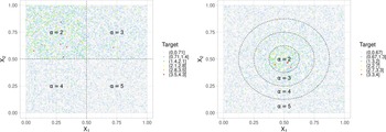
and the partition subsets are squares for Model 1 and parts of nested discs for Model 2. More specifically, the respective partitions
 $\mathcal{P}^{\left( 1\right) }$
and
 $\mathcal{P}^{\left( 2\right) }$
of
 $\mathcal{X}$
are of size 4 and are depicted in Figure 2.
Partitions
 $\mathcal{P}^{\left( 1\right) }$
and
 $\mathcal{P}^{\left( 2\right) }$
of
 $\mathcal{X}$
with their associated tail index values.

Geometric figures such as squares are a priori easily identified by gradient tree boosting algorithms. However, disks do not appear to be natural partitions for this type of algorithms. These two extreme cases will allow us to observe the efficiency of our approach for sets of partitions with potentially complex shapes.
Since the slowly varying functions of the family of conditional survival distribution functions of Z are equal to 1, it is not necessary to choose a family of thresholds for these datasets or to select observations whose values are higher than the thresholds. The sizes of the datasets are chosen to be equal to
 $n=50,000$
. The datasets
 $\mathcal{D}^{(1)}$
and
 $\mathcal{D}^{(2)}$
are given by the sets of values
 $\{\left( Z_{i},\mathbf{X}_{i}\right) _{i=1,\ldots ,n}\}$
for each model. In Figure 2, each point represents an observation (the color of a point is given by the value of its associated observation).
We choose the tail gradient tree boosting method to build the large-size partitions. The gradient tree boosting combines 100 weak tree learners. We performed a grid search with a 5-fold cross-validation to find a set of good hyper-parameters. We evaluated the performance of the models with the Gamma deviance. The values of the hyper-parameters are presented in Table 1 (see https://docs.h2o.ai/h2o/latest-stable/h2o-docs/data-science/gbm.html for the definitions of the hyper-parameters). We simulated test datasets with the same size to understand how the models generalize.
Choice of the hyper-parameters.

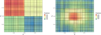
Figure 3 provides the large-size partitions obtained for
 $\mathcal{D}^{(1)}$
and
 $\mathcal{D}^{(2)}$
. The color inside a rectangle represents the value of the prediction of the Hill index function for this rectangle. The tail gradient tree boosting model performs well on
 $\mathcal{D}^{(1)}$
which is not surprising because the subsets of the partition
 $\mathcal{P}^{\left( 1\right) }$
are characterized by intersections of conditions that only depend on
 $X_{1}$
or
 $X_{2}$
, but not both. The learning task is more difficult and challenging for
 $\mathcal{D}^{(2)}$
because the subsets of the partition
 $\mathcal{P}^{\left( 2\right) }$
depend on an intricate way of
 $X_{1}$
and
 $X_{2}$
.
Tail gradient tree boosting partitions for
 $\mathcal{D}^{(1)}$
and
 $\mathcal{D}^{(2)}$
.

We then run ClustGeo to gather the rectangles of the tail gradient tree boosting partitions in order to reveal the partitions
 $\mathcal{P}^{\left( 1\right) }$
and
 $\mathcal{P}^{\left( 2\right) }$
. The matrix
 $D_{1}$
which gives the dissimilarities in the spatial space is defined in the following way: if two rectangles are adjacent, the distance value is set to
 $0.1,$
and if this is not the case, the distance value is set to a large value
 $d=9.10^{6}$
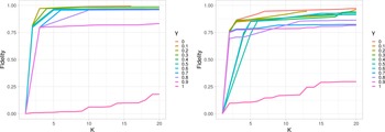
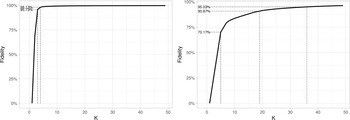
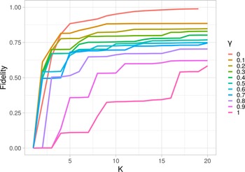
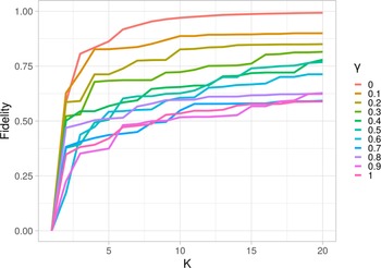
. Figure 4 shows the fidelity curves (which are defined as the curves of the
 $R^{2}$
measures between the aggregated partition and the initial partition created by the tail gradient tree boosting for different values of the weight parameter
 $\gamma \in \lbrack 0,1]$
). On the basis of these curves, we choose
 $\gamma = 0.3$
for
 $\mathcal{D}^{(1)}$
and
 $\gamma = 0.1$
for
 $\mathcal{D}^{(2)}$
, while fixing the size K of the small-size partitions to 4. The fidelity is then equal to
 $94.91$
% for
 $\mathcal{D}^{(1)}$
and
 $91.18$
% for
 $\mathcal{D}^{(2)}$
.
Fidelity curves for
 $\mathcal{D}^{(1)}$
and
 $ \mathcal{D}^{(2)}$
.

Estimated small-size partitions for
 $\mathcal{D}^{(1)}$
and
 $\mathcal{D}^{(2)}$
.

QQ-plots comparing the distributions of the normalized observations inside each subsets of the estimated partitions with the unit Exponential distribution.

Fidelity curves of the equivalent tree models for
 $\mathcal{D}^{(1)}$
and
 $\mathcal{D}^{(2)}$
.

Approximated small-size partitions of the equivalent tree models for
 $\mathcal{D}^{(1)}$
and
 $\mathcal{D}^{(2)}$
.

QQ-plots comparing the distributions of the normalized observations inside each subsets of the estimated partitions with the unit Exponential distribution.

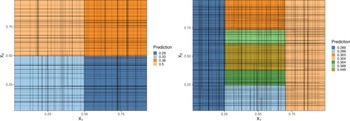
Figure 5 provides the estimated small-size partitions for
 $\mathcal{D}^{(1)}$
and
 $\mathcal{D}^{(2)}$
. For
 $\mathcal{D}^{(1)}$
, we observe that the hierarchical clustering algorithm has some difficulties in separating the region where the Hill index is equal to
 $0.2$
from the one where it is equal to
 $0.25$
. This reason is that these values are actually too close. Moreover, it creates a fourth small subset for the partition in the region where the Hill index is equal to
 $0.25$
without providing a very different predicted value. A partition with three subsets would therefore be sufficient here. Nevertheless, the shapes of the estimated subsets of the partition are close to the shapes of the true subsets. For
 $\mathcal{D}^{(2)}$
, we observe that the circular subsets for the tail indexes equal to
 $0.25$
,
 $0.33$
and
 $0.5$
are relatively well estimated, but the subset for the value
 $0.25$
is the union of two disjoint subsets. We conclude that ClustGeo does a good job for identifying the small-size partitions.
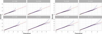
In Figure 6, QQ-plots compare the distributions of the normalized observations inside each subsets of the estimated partitions (they have been divided by their mean) with the unit Exponential distribution. The alignment of the points in the 95% pointwise confidence intervals (based on order statistics of the unit Exponential distribution) shows good fits and validates the assumption of Exponential distributions for
 $\log \!\left( Z\right) $
. The tail indexes for the orange and yellow subsets are very well estimated.
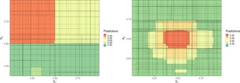
Finally, we compare the estimated partitions with the outputs of the equivalent tree model. Figure 7 provides the fidelity curves (
 $R^{2}$
measure) between the approximated partitions and the initial partition created by the tail gradient tree boosting. We decide to choose
 $K=4$
subsets for
 $\mathcal{D}^{(1)}$
with a high fidelity (
 $98.10$
%) and
 $K=7$
subsets for
 $\mathcal{D}^{(2)}$
with a good fidelity (
 $79.24$
%). Figure 8 shows the approximated small-size partitions for
 $\mathcal{D}^{(1)}$
and
 $\mathcal{D}^{(2)}$
. The equivalent tree model provides the exact partition for
 $\mathcal{D}^{(1)}$
, doing better than the hierarchical clustering algorithm. Although the approximated small-size partition differs from the true one for
 $\mathcal{D}^{(2)}$
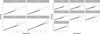
, the explanations that could be made would be very convincing. In Figure 9, QQ-plots compare the distributions of the normalized observations inside each subsets of the approximated partitions with the unit Exponential distribution. The alignment of the points also shows good fits.
3.2. A case study for the insurance industry
We consider a NOAA tornado dataset containing 60,652 events from 1950 to 2011. The variables that we kept from this dataset are given in Table 2 (the other variables were quantitative variables with too many missing values or categorical variables). We combined the variables PROPDMGEXP and PROPDMG to a single variable PROPERTY DAMAGE containing the estimated costs (in dollars) of the damages caused by tornadoes. We only retained strictly positive amounts of PROPERTY DAMAGE and ended up with 39,036 observations. We finally extracted YEAR and MONTH from the variable DATE.
Descriptive table of variables.

We are interested in characterizing the extremal behavior of property damages caused by tornadoes. The documentation provided with the dataset does not mention whether inflation has been taken into account to evaluate property damages, but after analyzing the amounts of damages, we concluded that it was not the case and decided to adjust these amounts for inflation (we used the historic American inflation based upon the consumer price index because it was the only index with a large enough history). We also decided to add contextual information about the population densities since the damages caused by tornadoes are correlated to the human constructions in the area they strike. We used a shapefile containing geographical frontiers of US counties that we linked with the census data to extract population densities by year and county (DENSITY) (we did not have information on the populations affected by the tornadoes, and therefore, we assumed that the affected population densities were proportional to the population densities). We thereafter consider as our variable of interest the following variable: DAMAGE BY DENSITY
 $=$
PROPERTY DAMAGE DENSITY.
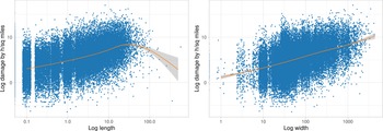
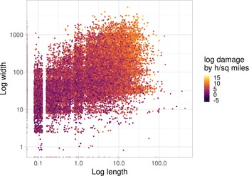
Figure 10 illustrates the linear relationships between
 $\log \!\left( \text{DAMAGE BY DENSITY}\right) $
with respectively
 $\log \!\left( \text{LENGTH}\right) $
and
 $\log \!\left( \text{WIDTH}\right) $
, while Figure 11 provides a scatter plot showing that the longer and the wider a tornado track, the greater the damage will be.
Linear relationships between
 $\log \!\left( \text{DAMAGE BY DENSITY}\right) $
with respectively
 $\log \!\left( \text{LENGTH}\right) $
and
 $\log \!\left( \text{WIDTH}\right) $
.

Scatter plot of
 $\log \!\left( \text{LENGTH}\right) $
and
 $\log \!\left( \text{WIDTH}\right) $
.

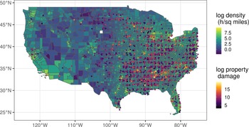
Figure 12 displays a map of the United States with the population density per county as well as the locations of a random subsample of the tornadoes depicted with different colors depending on the amount of damages.
Population density in the US and tornado locations.

After a detailed study of the tails of the distributions of the variable DAMAGE BY DENSITY, we concluded that it was necessary to make a deterministic transformation of this variable so that the observations are compatible with the hypothesis of a Pareto-type distribution. The tails of the distributions are in fact of Weibull-type with a coefficient
 $\theta $
that can be estimated following the approach developed in Girard (Reference Girard2004). The values of the estimators of the Weibull tail-coefficient
 $\hat{\theta}_{n}$
based on the
 $k_{n}$
upper order statistics are given in the left panel of Figure 13. In practice, the choice of the parameter
 $k_{n}$
is the key problem to obtain a correct estimation of
 $\theta $
. If
 $k_{n}$
is too small, the variance of
 $\hat{\theta}_{n}$
may be high and conversely, if
 $k_{n}$
is too large, the bias may be important. We retained the approach proposed in Girard (Reference Girard2004) and selected the values
 $k_{n}=5000$
and
 $\hat{\theta}_{n}=4$
. Therefore, we transform the variable DAMAGE BY DENSITY in the following way
 \begin{equation*}Z=\exp \!\left( \left( \text{DAMAGE BY DENSITY}\right)^{1/4}\right) .\end{equation*}
Figure 13 displays a QQ-plot comparing the distribution of
 $Y=\log \!\left(Z\right) $
with an Exponential distribution. It should be kept in mind that the threshold exceedance distribution of Y is expected to be a mixture of Exponential distributions with different parameters in different subsets of the covariate space. It is therefore not possible to obtain a perfect alignment of the points as in the case of a simple Exponential distribution. However, this graph allows us to think that the choice of
 $\hat{\theta}_{n}$
is consistent with our working hypothesis.
Left panel: Weibull tail-coefficient estimator
 $\hat{\theta}_{n}$
; Right panel: QQ-plot comparing the distributions of the observations with the Exponential distribution.

The covariates that have been retained for building an additive tree model are MAG, LENGTH, WIDTH, LATITUDE, LONGITUDE, YEAR. We divided the observations into two subsets : a training set (80% of observations) and a validation set (20% of observations). As mentioned previously, we chose the threshold function for which the function t is uniformly constant per region where the regions were obtained from products of median class intervals of the covariates. In a first step, we fitted several tail gradient tree boosting models on all the data with not optimized hyper-parameters to choose the best threshold function. The selected threshold function was the one that retains 90% of the largest values in each region. Then, we fitted again tail gradient tree boosting models on the subset of data to optimize the values of the hyper-parameters. The choice of the hyper-parameters are given in Table 3.
The grid search for the hyper-parameters was performed with a 5-fold cross-validation. We selected the model with the smallest Gamma deviance, and we denote by GBM Gamma this model (the Gamma deviance on the train set is equal to
 $0.8389$
, on the validation set
 $0.8488$
and by cross-validation
 $0.8422$
).
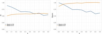
We then run ClustGeo to gather subsets of the tail gradient tree boosting partition. We first choose
 $D_{1}$
as the distance which is set to
 $0.1$
if two rectangles are adjacent and to a large value if this is not the case. To help us choose the mixing parameter
 $\gamma $
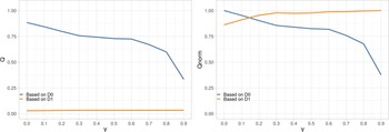
, we plot the proportions (resp. normalized proportions) of explained pseudo-inertia of the partitions in K clusters obtained with the ClustGeo procedure for a range of
 $\gamma $
(the pseudo-inertia of a cluster is calculated from the dissimilarity matrix and not from the data matrix). When the proportion (resp. normalized proportion) of explained pseudo-inertia based on
 $D_{0}$
decreases, the proportion (resp. normalized proportion) of explained pseudo-inertia based on
 $D_{1}$
increases. The plots are given in Figure 14.
We also compute the fidelity curves with respect to
 $\gamma$
(see Figure 15). On the basis of these plots, we choose
 $\gamma = 0.1$
and
 $K=12$
(
 $R^{2}$
measure is equal to
 $88.38$
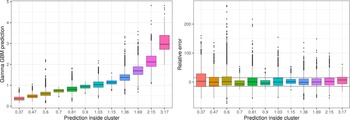
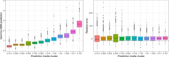
%.). Figure 16 displays box plots of the predicted values by GBM Gamma for each subset of the estimated partition, as well as box plots of their relative differences with their averages (i.e., by taking the averages as the reference values). For almost every subsets, more than 50% of the predictions have relative differences less than 15% in absolute value.
Selected model.

Proportions (resp. normalized proportions) of explained pseudo-inertias according to
 $\gamma $
in the left panel (resp. in the right panel).

Fidelity curves according to
 $\gamma $
.

Left panel: GBM Gamma predictions by subset of the partition; Right panel: Relative differences.

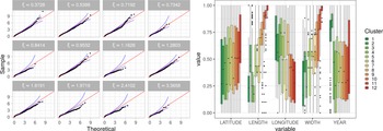
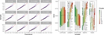
We finally provide in the left panel of Figure 17 the QQ-plots comparing the distributions of the normalized observations inside each subsets of the estimated partitions with the unit Exponential distribution and in the right panel the box plots of the predicted values for each subset of the estimated partitions and for the covariates: LATITUDE, LENGTH, LONGITUDE, WIDTH, YEAR. We note that the empirical distributions inside the subsets of the estimated partition are not all well approximated by Exponential distributions. We observe that the covariates LENGTH and WIDTH are the covariates that most influence the means of observations through the subsets of the estimated partition.
Left panel: QQ-plots comparing the distributions of the normalized observations inside each subset of the estimated partitions with the unit Exponential distribution; Right panel: Box plots of the predicted values for each subset of the estimated partitions and for the covariates:
 $\text{LATITUDE, LENGTH, LONGITUDE, WIDTH, YEAR}$
.

Proportions (resp. normalized proportions) of explained pseudo-inertias according to
 $\gamma $
in the left panel (in the right panel).

Fidelity curves according to
 $\gamma $
.

For
 $D_{1}$
, we now take the Euclidean distance between the gravity centers of the rectangles. We obtain Figures 18 and 19.
On the basis of these plots, we chose
 $\gamma = 0.1$
and
 $K=12$
(the
 $R^{2}$
measure is equal to
 $89.44$
%.). Figure 20 displays box plots of the predicted values by GBM Gamma for each subset of the estimated partition, as well as box plots of their relative differences with their means. The ranges of the box plots are slightly larger than for the non-Euclidean distance.
Left panel: GBM Gamma’s predictions by subset of the partition; Right panel: Relative errors.

Left panel: QQ-plots comparing the distributions of the normalized observations inside each subset of the estimated partitions with the unit Exponential distribution; Right panel: Box plots of the predicted values for each subset of the estimated partitions and for the covariates:
 $\text{LATITUDE, LENGTH, LONGITUDE, WIDTH, YEAR}$
.

Fidelity curve.

We also provide in the left panel of Figure 21 the QQ-plots comparing the distributions of the normalized observations inside each subsets of the estimated partition with the unit Exponential distribution and in the right panel the box plots of the predicted values for each subset of the estimated partitions and for the covariates: LATITUDE, LENGTH, LONGITUDE, WIDTH, YEAR. The assumption of an Exponential distribution for each subset of the partition is now more convincing. Moreover, the box plots provide evidence of clearer links between the covariates considered and the empirical distributions of the observations through the subsets.
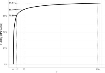
We finally consider the Equivalent tree method. Figure 22 displays the fidelity curve which led us to also choose
 $K=12$
subsets with the
 $R^{2}$
measure equal to
 $75.89$
%.
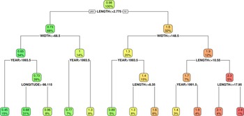
The tree that leads to the approximated partition is depicted in Figure 23. The covariates LENGTH and WIDTH appear to be the most discriminating variables. The year 1993 also appears to be an important year because a significant change in the tail index can be observed before and after this year. A comparison with the regression tree obtained by the methodology developed in Farkas et al. (Reference Farkas, Lopez and Thomas2021) is presented in Appendix B.
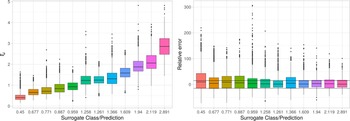
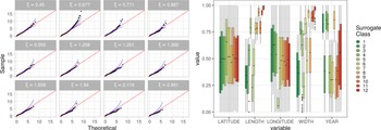
Figure 24 provides box plots of the predicted values by the equivalent tree for each subset of the estimated partition, as well as box plots of their relative differences with their averages. Figure 25 shows that the approximated partition of the equivalent tree gives distributions of normalized observations inside each subset that are relatively close to the unit Exponential distribution.
Surrogate tree (
 $R^{2} = 75$
%).

Left panel: Equivalent tree predictions by subset of the partition; Right panel: Relative errors.

Left panel: QQ-plots comparing the distributions of the normalized observations inside each subset of the estimated partitions with the unit Exponential distribution; Right panel: Box plots of the predicted values for each subset of the estimated partitions and for the covariates:
 $\text{LATITUDE, LENGTH, LONGITUDE, WIDTH, YEAR}$
.

From these different analyses, we can draw the following conclusions:
-
– The small-size partition obtained from the additive tree ensemble and the hierarchical clustering with spatial constraints based on the Euclidean distance has a better fidelity than the one obtained with the tree surrogate model for the same number of classes.
-
– But the empirical distributions of the observations within each subset of the partitions are even so close to Exponential distributions for the tree surrogate model while providing natural explanations for the classes in terms of covariates and a simple division of the covariate space.
4. Conclusions
Estimating the tail index can become highly complex in the presence of covariates in order to gain a competitive advantage in risk assessment. However, providing simple but accurate models is a key requirement for any high-stakes decision. In this paper, we assume that the tail index function only takes a small number of values over a partition of the covariate space. We propose a tail-index partition-based rules extraction method that is able to construct estimates of the partition subsets and estimates of the tail index values.
The method combines two steps: first an additive tree ensemble based on the Gamma deviance is fitted (which includes random forest and gradient tree boosting), and second a hierarchical clustering with spatial constraints (ClustGeo) is used to estimate the subsets of the partition. The number of subsets of the partition is selected first by determining a weight coefficient between the dissimilarity matrices that provides a high degree of spatial contiguity without deteriorating too much the quality of the solution based only on the predictions of the additive tree ensemble, second by ensuring a sufficiently high level of fidelity (
 $R^{2}$
measure). The quality of the choice of the partition is finally checked by comparing the fit of the distributions of the observations to Exponential distributions with QQ-plots for each subset of the partition.
Our procedure provides a small number of subsets of the covariate space whose shape may be however highly complex because they were constructed with constraints to form homogeneous subsets in terms of predictions but also homogeneous in the covariate space. It may be difficult to find simple covariate-based explanations for these subsets. We have therefore proposed a global tree surrogate model to approximate the partition-based rules while providing an explainable model from the initial covariates. If explanations are to be provided, fidelity should be sacrificed in order to generate a more “ rigid” model with cuts aligned with the covariate axes. Our numerical experiments as well as the case study show that the drop in quality is actually not that great.
Acknowledgments
The authors acknowledge three referees for their remarks and comments which greatly enhanced the relevance of this paper.
R code and database
The code for the tail gradient tree boosting and the database considered for the case study are made publicly available at https://bitbucket.org/_semicroustillant_/tail-index-partition-based-rules-extraction/src/master/.
Appendix
A. A comparison of threshold selection methods for the tail gradient boosting algorithm
In this section, we consider two threshold functions
 $t_{u}\!\left( \mathbf{\cdot }\right) = ut\!\left( \mathbf{\cdot }\right) $
, discuss the choice of the threshold constant u and compare their performances for the tail gradient boosting algorithm. The two threshold functions,
 $t_{u}\!\left( \mathbf{\cdot }\right) $
, are chosen in the following way: (i) a uniformly constant function
 $t\!\left( \mathbf{\cdot }\right) $
over
 $\mathcal{X}$
and u satisfying for some
 $\gamma \in (0,1)$
,
 \begin{equation*}\int_{\mathcal{X}}P\!\left( \left. Z>t_{u}\!\left( \mathbf{x}\right) \right\vert\mathbf{X}=\mathbf{x}\right) dP_{\mathbf{X}}\!\left( \mathbf{x}\right)=1-\gamma ,\end{equation*}
and (ii) a piecewise constant function
 $t\!\left( \mathbf{\cdot }\right) $
over a partition
 $\left( \mathcal{X}_{i}\right) $
of
 $\mathcal{X}$
and u satisfying for some
 $\gamma \in (0,1)$
,
 \begin{equation*}\int_{\mathcal{X}_{i}}P\!\left( \left. Z>t_{u}\!\left( \mathbf{x}\right)\right\vert \mathbf{X}=\mathbf{x}\right) dP_{\mathbf{X}}\!\left( \mathbf{x}\right) = 1-\gamma ,\qquad \text{for all }\mathcal{X}_{i}\subset \mathcal{X}.\end{equation*}
We present a simulation study where
 $p=2$
,
 $\mathcal{X}=[0,1]\times \lbrack0,1]$
,
 $X_{1}$
and
 $X_{2}$
are two independent random variables uniformly distributed over [0, 1], the partition of
 $\mathcal{X}$
is given by
 $\mathcal{X}_{ij}=[(i-1)/10,i/10]\times \lbrack (j-1)/10,j/10]$
for
 $i,j=1,\ldots ,10$
and
 \begin{equation*}\alpha \!\left( x_{1},x_{2}\right) = \left( 1+\frac{x_{1}}{2}\right) \left(4-2x_{2}\right) ,\qquad x_{1},x_{2}\in \lbrack 0,1].\end{equation*}
Figure A.1 provides a color-level plot of this function.
Color-level plot of the tail index function.

Moreover, as in Wang and Tsai (Reference Wang and Tsai2009), we assume that, for some
 $m\geq 0$
,
 \begin{equation*}P\!\left( \left. Z>z\right\vert \mathbf{X}=\mathbf{x}\right) = \frac{\left(1+m\right) z^{-\alpha \left( \mathbf{x}\right) }}{1+mz^{-\alpha \left(\mathbf{x}\right) }},\quad z>0,\mathbf{x}\in \mathcal{X},\end{equation*}
and hence
 \begin{equation*}L\!\left( z;\;\mathbf{x}\right) = \left( 1+m\right) -m\!\left( m+1\right)z^{-\alpha \left( \mathbf{x}\right) }+o\!\left( z^{-\alpha \left( \mathbf{x}\right) }\right) ,\quad \text{as }z\rightarrow \infty .\end{equation*}
The parameter m measures the deviation from the model where the slowly varying functions
 $L\!\left( z;\;\mathbf{x}\right) $
are constant. When
 $m=0$
, all data must be kept because
 $\ln\!(Z)$
given
 $\mathbf{X}=\mathbf{x}$
has an Exponential distribution. When m increases, a larger threshold must be selected to be closer to this Exponential model condition.
Since the distribution of
 $\alpha \!\left( \mathbf{x}\right) Y^{(u)}=\alpha\!\left( \mathbf{x}\right) \ln \!\left( Z/t_{u}\!\left( \mathbf{x}\right) \right) $
conditional on
 $Z>t_{u}\!\left( \mathbf{x}\right) $
and
 $\mathbf{X}=\mathbf{x}$
is approximately a unit Exponential distribution, the distribution of
 $U^{(u)}=\exp \!\left(-\alpha \!\left( \mathbf{x}\right) Y^{(u)}\right) $
conditional on
 $Z>t_{u}\!\left( \mathbf{x}\right) $
is approximately a uniform distribution on [0, 1]. Depending on the choice of the threshold function, the approximation will be more or less accurate. If the sample fraction of the data is too small because the threshold is too high, the conditional distribution of
 $U^{(u)}$
can be well approximated by the uniform distribution on [0, 1], but could result in greater estimation errors between
 $\alpha$
and
 $\alpha _{M,n}^{\left( u\right),g}$
where
 $\alpha _{M,n}^{\left( u\right) ,g}=1/\xi_{M,n}^{\left( u\right) ,g}$
. If the sample fraction gets large because the threshold is low, the approximation of the conditional distribution of
 $U^{(u)}$
is less accurate, and therefore, there could be a large discrepancy between the uniform distribution on [0, 1] and the empirical distribution of
 $\{\hat{U}_{i}^{(u)}\;:\;Z_{i}>t_{u}\!\left( \mathbf{X}_{i}\right) \}$
with
 $\hat{U}_{i}^{(u)}=\exp\!(\!-\!\alpha _{M,n}^{\left(u\right) ,g}\left( \mathbf{X}\right) Y_{i}^{(u)})$
. As a consequence, the choice of the threshold function may be made by choosing the sample fraction that produces the smallest discrepancy between the empirical distribution of
 $\{\hat{U}_{i}^{(u)}\;:\;Z_{i}>t_{u}\!\left( \mathbf{X}_{i}\right) \}$
and the uniform distribution on [0, 1]. The discrepancy measure that we retain is given by
 \begin{equation*}\hat{d}\!\left( u;\;t\!\left( \mathbf{\cdot }\right) \right) = \frac{1}{n^{(u)}}\sum_{i\in \mathcal{I}_{n}^{(u)}}\left( \hat{U}_{(i)}^{(u)}-\frac{i}{n^{(u)}}\right) ^{2}\end{equation*}
where
 $(\hat{U}_{(i)}^{(u)})_{i\in \mathcal{I}_{n}^{(u)}}$
is the order statistics of
 $(\hat{U}_{i}^{(u)})_{i\in \mathcal{I}_{n}^{(u)}}$
. If
 $\{\hat{U}_{i}^{(u)}\;:\;Z_{i}>t_{u}\!\left( \mathbf{X}_{i}\right) \}$
is a sample of uniformly distributed random variables, then
 $\hat{U}_{(i)}^{(u)}$
should be close to
 $i/n^{(u)}$
and
 $\hat{d}\!\left( u;\;t\!\left( \mathbf{\cdot }\right)\right) $
should be small. This suggests that u is chosen to minimize
 $\hat{d}\!\left(u;\;t\!\left( \mathbf{\cdot }\right) \right) $
.
In our study, we consider three sample sizes (
 $n=4,000; 10,000; 20,000$
) and three m values (
 $m=0.15;\;0.3;\;0.6$
). In addition, 500 simulation realizations are conducted for each model setup.
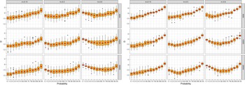
Figure A.2. provides boxplots of
 $\hat{d}\!\left( u;\;t\!\left( \mathbf{\cdot }\right) \right) $
for the two strategies (i) the uniformly constant function and (ii) the uniformly constant function per region.
Boxplots of
 $\hat{d}\!\left( u;\;t\!\left( \mathbf{\cdot }\right) \right) $
for different values of the probability
 $\gamma $
for the uniformly constant function (Left panel) and the uniformly constant function per region (Right panel).

The choice of u (and thus
 $\gamma $
) that minimizes
 $\hat{d}\!\left(u;\;t\!\left( \mathbf{\cdot }\right) \right) $
depends on the value of m and
 $n$
. The larger m is, the larger u and
 $\gamma $
are. We can also see that, as n increases, u and
 $\gamma $
increase slightly, but less than u. This means that the algorithm retains a higher threshold, but at the same time retains more data (although less in proportion). The criterion of choosing the threshold tends to select only the most relevant data. The results are essentially the same for both strategies, that is (i) the uniformly constant function and (ii) the uniformly constant function per region. The choices of the thresholds are more or less the same, but the levels of
 $\hat{d}\!\left( u;\;t\!\left( \mathbf{\cdot }\right) \right) $
for the optimal
 $u^{\ast }$
are lower for strategy (ii). We therefore retain strategy (ii).
Color-level plots of the bias of
 $\alpha _{M,n}^{\left( u^{\ast }\right) ,g}$
.

Color-level plots of the bias of the RMSE of
 $\alpha _{M,n}^{\left(u^{\ast }\right) ,g}$
.

Once the choice of threshold has been made, it is possible to study the bias and RMSE of the estimator
 $\alpha _{M,n}^{\left( u^{\ast }\right) ,g}$
(see Figures A.3 and A.4). Naturally, the bias and the RMSE tend to increase as m increases, but decrease as n increases. The area where the estimator is the worst corresponds to the area where
 $\alpha$
takes its highest values, around 6. As soon as n exceeds 10,000, the bias becomes small and almost negligible for n larger than 20,000. The RMSE is uniformly smaller than
 $0.5$
for
 $n=20,000$
whatever the value of m, which shows the excellent precision of the algorithm.
B. A comparison of the Surrogate tree with the regression tree of Farkas et al. (Reference Farkas, Lopez and Thomas2021)
This subsection provides a comparison with the regression tree obtained by the methodology developed in Farkas et al. (Reference Farkas, Lopez and Thomas2021). In this paper, the authors combine a Generalized Pareto modeling and a regression tree approach. More specifically, they replace the quadratic losses used in the “growing” phase of Breiman’s regression tree with the additive inverses of log-likelihoods of Generalized Pareto distributions.
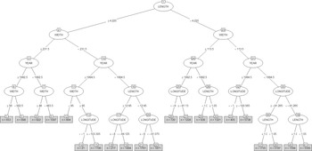
We used the same database as in Section 3.2 (i.e., the database for which the threshold function retained 90% of the largest observations in each region). The regression tree of Farkas et al. (Reference Farkas, Lopez and Thomas2021) obtained after pruning is given in Figure B.1 while variable importance can be found in Table B.1. The regression tree of Farkas et al. (Reference Farkas, Lopez and Thomas2021) has 21 terminal leaves, which is larger than the Surrogate tree which has 12 terminal leaves.
Regression tree of Farkas et al. (Reference Farkas, Lopez and Thomas2021).

Variable Importance for the regression tree of Farkas et al. (Reference Farkas, Lopez and Thomas2021).

Hill coefficient values
 $\alpha _{i}$
per leaf.

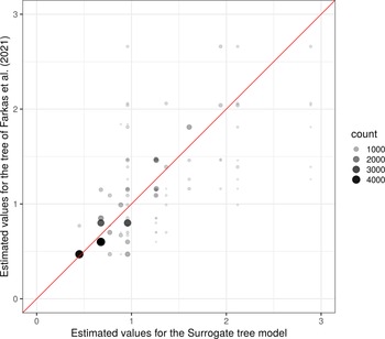
Comparison of estimated values between the Surrogate tree and the regression tree of Farkas et al. (Reference Farkas, Lopez and Thomas2021).

As for the Surrogate tree, covariates LENGTH, WIDTH and YEAR are the most important covariates for the construction of the first leaves of the tree. Covariate LONGITUDE is also mainly used for the terminal leaves. Note however that the levels of the covariates retained for the splits can be quite significantly different between the two methods.
The values of the Hill coefficient
 $\alpha _{i}$
are given in Table B.2 for each terminal leave. These values are compared with those of the Surrogate tree in Figure B.2.