MANYinvestigations have confirmed Reference WegenerWegener's (1912) suggestion that on geological time-scales the various continents "drift" from one position to another on the surface of the Earth (e.g. Reference Vine and MatthewsVine and Matthews, 1963; Reference WestollWestoll, 1965). Maps are now available (Reference Smith and BridenSmith and Briden, 1977; Reference SchmidtSchmidt, 1988) which purport to trace the positions of the continents as far back as 600 Ma. Considering only the last 150 Ma for which the positional evidence from palaeore construction is reasonably solid, there was a break-up of Gondwana in the Southern Hemisphere (effectively, Wegener's "flight from the pole" of South America, South Africa, India and Australia) and a break-up of Laurasia in the Northern Hemisphere as Eurasia and North America moved away from one another to form the Atlantic Ocean. The mechanism for continental drift is presumably related to large-scale convection in the Earth's mantle (Reference Peltier and PeltierPeltier, 1989; Reference Olson, Silver and CarlsonOlson and others, 1990). One qualitative picture is of a fluid but highly viscous mantle in which up-wellings and down-wellings generate horizontal flows at its surface which carry the floating continental plates. The source of the convection is generally assumed to be differential heating from the core. Divergence of the plates is most clearly seen in the patterns of magnetic anomalies developed at the spreading mid-ocean ridges (e.g. Reference Veevers, Powell and RootsVeevers and others, 1991).

Since the early work of Reference WalcottWalcott (1973),Reference CathlesCathles (1975) and others, there have been many studies of the vertical displacement and subsequent isostatic rebound of those continental plates (or parts of plates) which are subject to extra loading by ice sheets during periods of glaciation. It is largely from these studies that information on the elasticity and rigidity of the lithosphere, and on the vertical profile of viscosity in the mantle, are derived. This note points out that the horizontal components of flow in the mantle induced by the regular (?) cycling of ice-sheet loading and unloading may be of the same order as the observed velocities of continental drift, i.e. some cm a¹ . Thus, given some non-linear mechanism which ensures preferential movement in the one direction, it is possible, at least for those periods of the Earth's history including the Quaternary when there was significant glaciation, that there could be a climatically induced element to continental drift.

(Fig. 1) shows the theoretical south to north flow rates of the surface of the upper mantle as a function of latitudeat various times during a single 30 ka cycle of ice-sheet loading and unloading of the Antarctic continent. The flow rates were calculated using a very simple "2¹/₂dimensional" numerical model with parameters as described in the caption to the figure. It envisages a horizontally uniform upper mantle whose viscosity varies with depth z according to the calculations of Reference CathlesCathles(1975); namely, 1.0 x lO²² Poise at all depths down to 1000 krn except for a low-visrosity channel (4.0 x 10²⁰ Poise) in the uppermost 100 km. The continental plate corresponding to Antarctica is imagined to float on the mantle from the South Pole to 70^° S, and the rest of the mantle has a free surface at z = O. The mantle rnaterial is assumed to be inelastic, incompressible and Newtonian. The imposed ice-sheet cycle is a sinusoidal height variation with an amplitude of 1000 m, about half the present thickness of the ice on Antarctica.

Fig. 1.

Computed mantle elevation H (dashed lines) and south to north mantle-suifaceflow rates v (solid lines) as a function of latitude x at various times t in a single 30 ka cycle of ice-sheet loading of Antarctica, according to the fol101ting numerical model which solves the one-dimensional steady-state viscous- flow equation dp/dx = #x000E2;#x020AC;#x201D;#x000F0;œ‡(z)d² v /dz². Grid spacing: 225 intervals of latitude from South to North Pole, 20 depth levels fiom Z = 0 to z = Z_d = lOOO km, oneinterval in the east-west (y) direction of unit width at the Equator but varying as cos x. Viscosity profile ðœ‡.(z) as given in the text. Excess pressure p due to imposed ice load on Antarctica (from x = -90° to -70°) = po(x,t) =ðœŒgh(t) where h(t) = h0- h0cos(2𜋠.t/ 30000) with h0= 1000 m, g =acceleration due to gravity and ðœŒ= density of ice = 1000 kg m^-3. Viscous transfer in the horizontal direction is translated into mantle elevation H(x) and hence excess pressure assuming densitv of mantle = 4000 kg m³ . Flow-boundaryconditions of >v (x,z_d ) = 0, >v (x, O) = 0 at all x .from -90° to 70°, dv/dz = 0 elsewhere. The time step was 1 year.

The choice of a 30 ka cycle for the illustrative purpose of (Fig. 1) was not random. During prolonged periods of the Earth's glaciation the volume of ice fluctuates on various time-scales with, at least over the last 700 ka, readily observable periods of the order of 20, 40 and 100 ka. They appear to be related to orbital variations of the Earth about the Sun (Reference Van WocrkumVan Woerkum, 1953; Reference Raymo, Ruddiman, Shackleton and OpppRaymo and others, 1990). The last major glacial cycle in the Northern Hemisphere was of the order of 100ka, and much of the work on isostatic rebound (e.g. Reference Tushingham and PeltierTushingham and Peltier, 1991) has assumed a build-up and decay of ice volume over a period of that order. Significant modulation of ice volume at the shorter time-scales occurred during that and previous cycles, and the illustrative 30 ka cycle was chosen here simply as an order-of-magnitude representation of those shorter time-scales.

(Fig. 1) reflects the obvious response to extra pressure on Antarctica. Material of the mantle is squeezed from beneath the plate to create a surface sloping downward towards the north and a horizontal component of velocity which at any latitude is a maximum at the surface and which (during the loading part of the cycle) decreases with distance along the great circle away from the Antarctic source. The relaxation-time constant of the model system is about 18ka (this is from calculations with the model itself), so that during the later part of the cycle, when the load of ice is reducing, there is still a northward velocity at latitudes close to the North Polc.

The system as described is linear, so that flows in the mantle induced by the increased pressure beneath Antarctica during the loading part of the glacial cycle are reversed during the unloading part of the cycle. If the loading-unloading cycle is regularly repeated, the system settles down to a Form of steady stale where the average velocities over a complete cycle are zero. To propose that the icc-loading process is significant in the context of long-term continental drift requires one to propose also some form of non-linear hysteresis which favours now (or, at least, the actual movement of floating continental plates) in one direction. It is not difficult to suggest a number of possible mechanisms. It is very difficult to justify them. The simplest suggestion (more or less in line with the modern investigations of plate tectonics and the formation of mid-ocean ridges) is that magma from the mantle wells up into the opening between two diverging continental plates, where it cools and solidifies to a material which is highly resistant to compression but poorly resistant to expansion (Reference Jaeger and CookJaeger and Cook, 1976). A floating continent which is carried in one direction by horizontal flow in the mantle would therefore be restrained from moving backward when the flow in the mantle reverses. Perhaps the main attraction of the suggestion is that it might in principle be checkable, since it implies a component of continental drift which is intermittent on the time-scale of several tens ofthousands of years. Such checking would require, say, development of some technique for examining the Quaternary stratigraphic chronology of the mid-ocean ridges at a level of detail much greater than that allowed by present magnetic-reversal stratigraphy.

Setting aside questions about what might be the most appropriate profiles of density and viscosity to use in a model, the present calculations involve a number of gross simplifications. For instance, the depth of the model is confined to that of the upper mantle (about 1000 km )simply to give some "floor" at which to set a boundary condition of zero velocity. (There is some evidence (Bott, 1971)to suggest that convection does not penetrate the boundary between the lower and upper mantle, although this does not necessarily excuse the neglect in the present context of viscous flow in the lower mantle. In any event, a larger model depth would yield greater velocities at the surface.) For instance, again, the "free" mantle surface is equivalent to assuming that drag of the continental plates by mantle flow is a viable mechanism for drift (Reference Forsyth and UyedaForsyth and Uyeda. 1975).

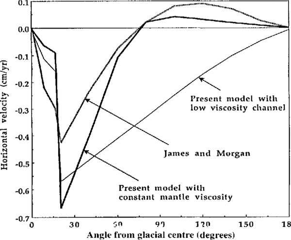
Despite the various simplifications, when the model is used to compute the present-day horizontal velocities associated with the most recent post-glacial rebound of North America, the results (see (Fig. 2)) are remarkably similar to those of Reference James and MorganJames and Morgan (1990), whose whole-Earth model includes specific consideration of such things as visco-elasticity of the mantle and rigidity of the lithosphere. The smaller velocity of the James and Morgan model near the ice-sheet edge is probably due to their (more realistic:') assumption of a parabolic height profile across the ice sheet, and to the smoothing effect of the lithosphere included in their model.

Fig. 2.

Present-day horizontal component of mantle—surface velocities (Positive away from the glacial centre) as a function of angular distance from the centre of the last North American ice sheet, which is assumed to have increased linearly in height from zero to a maximum (1km) over a period of 90ka, and decreased linearly back to zero by 100 ka(i.e. by 6000 a BP). The dashed curve is from the detailed model of James and Morgan (1990), the thick solid curve is from the present model with a constant mantleviscositvof 1.0 x 10²² Poise (as for James and Morgan), and the thin solid curve shows the effect of a low-viscosity channel as discussed in the reference to (Fig. 1).

(Fig. 3) shows computed average mantle-surface velocities where the averages at each latitude are taken over the loading half of a sinusoidal loading-and-unloading cycle. An increase of cycle time from 30 to 100 ka reduces the average velocities by a factor of 2, as might be expected anyway from consideration of the time constant of the svstem. If the low-viscosity channel is removed, so that all levels of the mantle have viscosity of 1.0 X 10²² Poise, the velocities at angular distances greater than 60° from the glacial centre (i.e. from the South Pole) are reduced to levels below 0.1 cm a^-1. The importance of the low-viscosity channel in determining the distribution of horizontal velocity is also apparent in the comparisons of (Fig. 2)

Fig. 3.

Time-averaged northward velocities for the "increasing load" half of a South Polar sinusoidal ice-sheet cycle. The curves refer to a 30 ka imposed cycle with a low-viscositv channel in the upper mantle (i.e. comparable with the conditions in (Fig. 1)), a 30 ka cycle with a constant mantle viscosity of l.0 x 10²² Poise and a 100 kacycle with a low-viscositv channel as in (Fig. 1).

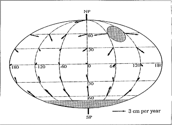
(Fig. 4) shows the geographical distribution of mantle-surface flow rates computed as the vector sum of the great-circle flow rates associated with ice loading of Antarctica and of a continent of equivalent size centered on 70°N. The picture is broadly (very broadly) consistent with the present movement of the continents, i.e. roughly south-north in the Southern Hemisphere and roughly east-west in the Northern Hemisphere. "Roughly" should be emphasized here. It can be gauged by reference to the known patterns of sea-floor spreading as, for instance, in Reference Press and SieverPress and Siever(1982). While the result in no way suggests that the mechanism suggested here is the primary cause of continental drift (either now or in glacial periods of the past), it is at least possible that the process amplifies certain directional components of an already established drift.

Fig. 4.

Geographical distribution of mantle-surface velocities for two ice sheets positioned as shown by shaded areas, each at 16 ka into an ice-loading cycle as in (Fig. 1) The calibration arrow outside the globe of length is equivalent to a velocity of 3.0 cm a^-1.

In summary, the existence of extended glacial periods on Earth seems to require a continent either to be very near a Pole or to have a significant fraction of its surface at high Elevation (Reference Budd and SmithBudd and Smith, 1979). The Earth has been largely ice-free for much of its history but, during glacial periods such as the Quaternary, the cyclical loading and unloading of ice may contribute significantly to continental drift. The main proviso is that there exists some non-linear mechanism associated with plate-mantle interaction which acts as a "ratchet" to ensure preferential movement of the continental plates in the one direction.