





1. Introduction
The mixing of fluids is a common process in nature and industry. The instantaneous mixing rate is controlled by the contact area between the fluids and the molecular diffusion coefficient,
 $D$
. In practice, mixing devices are devised to generate highly turbulent flows, where multi-scale eddies greatly increase the contact area (Dimotakis Reference Dimotakis2005). The T-shaped mixer is widely used because of its simple design and mixing efficiency (see e.g. Camarri et al. Reference Camarri, Mariotti, Galletti, Brunazzi, Mauri and Salvetti2020; Li & Xu Reference Li and Xu2023, for recent reviews). Despite its geometric simplicity, it displays a remarkably rich sequence of flow regimes as Reynolds number (
 $\textit{Re}$
) rises, ranging from symmetric laminar flow to the development of engulfment patterns and time-periodic symmetric oscillations (Hoffmann et al. Reference Hoffmann, Schlüter and Räbiger2006; Thomas et al. Reference Thomas, Ameel and Guilkey2010; Mariotti et al. Reference Mariotti, Galletti, Mauri, Salvetti and Brunazzi2018). Chaotic motion arises at
 $\textit{Re}\sim 500$
and the flow gradually turns turbulent as
 $\textit{Re}$
is further increased (Schikarski et al. Reference Schikarski, Peukert and Avila2017). The Reynolds number is defined as
 $\textit{Re}= {Ud}/{\nu }$
, where
 $U$
is the mean inlet velocity,
 $d$
the hydraulic diameter of the inlet and
 $\nu$
the kinematic viscosity of the fluid. In the specific geometry considered here, the outlet channel has aspect ratio
 $2$
and the mean outlet velocity is also
 $U$
.
Despite its prevalence in chemical engineering (Schwarzer et al. Reference Schwarzer, Schwertfirm, Manhart, Schmid and Peukert2006), the turbulent regime of T-mixers has been largely unexplored until recently. Schikarski et al. (Reference Schikarski, Trzenschiok, Peukert and Avila2019) studied the influence of the inlet conditions on the turbulent mixing for
 $\textit{Re} \leqslant 4000$
. They showed that by carefully manipulating the state of the inlet, the mixing rate could be greatly enhanced. For laminar inlets, they found that the turbulent statistics already became
 $\textit{Re}$
-independent at
 $\textit{Re}\gtrsim 2000$
. Recently, Li et al. (Reference Li, Asl, Bäuerlein, Avila, Xu and Avila2025) experimentally investigated mixing in a T-mixer with quasi-laminar inlets using particle image velocimetry and planar laser-induced fluorescence up to
 $\textit{Re}=5000$
. They measured turbulent kinetic energy (TKE) and scalar variance at three cross-sections along the outlet and provided evidence for the scaling of the scalar variance in the viscous-convective range predicted by Batchelor (Reference Batchelor1959) in the high-Schmidt number (
 $\textit{Sc}$
) limit.
Despite this recent progress, the mechanisms of turbulence generation and decay in T-mixers, and their impact on mixing, remain poorly understood. Here we fill this gap and examine the coherent structures and scaling of the turbulent quantities along the outlet up to
 $\textit{Re} = 2000$
and for laminar inlets. We relate our findings to established results of canonical turbulent flows, thereby shedding light on the physical mechanisms of turbulence in T-mixers.
2. Methods
2.1. Governing equations
The non-dimensional incompressible Navier–Stokes and scalar transport equations were solved to compute the fluid motion and mixing-
 \begin{equation} \frac {\partial \boldsymbol {u}}{\partial t} + \boldsymbol {u}\boldsymbol{\cdot }\boldsymbol{\nabla }\boldsymbol {u} = -\boldsymbol{\nabla }\!p + \frac {1}{\textit{Re}}\Delta \boldsymbol {u},\quad {\boldsymbol{\nabla }}\boldsymbol{\cdot }\boldsymbol {u}=0, \end{equation}
 \begin{equation} \frac {\partial {\theta }}{\partial t} + {\boldsymbol {u}}\boldsymbol{\cdot }\boldsymbol{\nabla }{\theta } = \frac {1}{\textit{ReSc}}\Delta {\theta }, \end{equation}
where
 ${\boldsymbol {u}}$
,
 $p$
, and
 $\theta$
denote the velocity, pressure, and scalar fields, respectively. Figure 1 illustrates the geometry and dimensions of the simulated T-mixer. We use Cartesian coordinates, with the origin positioned at the cente of the junction. The
 $y$
-axis is aligned with the opposing square duct inlet, while the
 $x$
-axis is oriented along the streamwise direction of the rectangular outlet duct. Lengths were non-dimensionalised with the hydraulic diameter of the inlets,
 $d$
, and velocities with the bulk velocity,
 $U$
. The Reynolds number in (2) and (3) is defined as
 $\textit{Re}= {Ud}/{\nu }$
, where
 $U$
is the mean inlet velocity,
 $d$
is the hydraulic diameter of the inlet and
 $\nu$
is the kinematic viscosity of the fluid. The Schmidt number
 $\textit{Sc}={\nu }/{D}$
, where
 ${D}$
is the molecular diffusion coefficient, was set to
 $\textit{Sc}=1$
.
Schematic of the computational domain.

Fully developed flow in a square duct was used as the boundary condition at the inlets of the T-mixer. (a) Colour map of the streamwise velocity. (b) Velocity profile at mid-height (
 $z=0$
). The dashed green line is from Schikarski et al. (Reference Schikarski, Trzenschiok, Peukert and Avila2019).

2.2. Boundary conditions
At the inlets, a fully developed laminar velocity profile for a square duct (Shah & London Reference Shah and London2014) was imposed as the boundary condition. In dimensionless form, it reads
 \begin{equation} u(x,z)=-\frac {4c_{1}}{\pi ^3}\sum _{n=1,3,\ldots }^{\infty }\frac {1}{n^3}(-1)^{\frac {n-1}{2}}\left [ 1-\frac {\cosh (n\pi x)}{\cosh \left(\dfrac {n\pi }{2}\right)} \right ]\cos (n\pi z), \end{equation}
where the constant
 \begin{equation} c_{1}=-\frac {12}{\left [ 1-\dfrac {192}{\pi ^5}\sum _{n=1,3,\ldots }^{\infty }\dfrac {1}{n^5}\tanh \left(\dfrac {n\pi }{2}\right) \right ]} \end{equation}
ensures that
 $\int _{- ({1}/{2})}^{ {1}/{2}}\int _{-( {1}/{2})}^{ {1}/{2}} u(x,z){\rm d}x{\rm d}z=1$
. Here
 $n$
is odd summation index. A colour map of the velocity figure 2(a) and profile at
 $z=0$
figure 2(b) obtained by a truncation of
 $n=5$
are shown in figure 2. A stabilised outflow boundary condition was applied at the outlet to prevent any backflow into the domain (Dong et al. Reference Dong, Karniadakis and Chryssostomidis2014). The no-slip boundary condition was applied at the walls. The scalar concentration was set to
 $\theta =1$
at the left inlet and
 $\theta =0$
at the right inlet, whereas homogeneous Neumann conditions,
 $ {\partial \theta }/{\partial n}=0$
, were applied at the walls and outlet. To compare the T-mixer outlet with a fully developed duct flow, we additionally performed simulations of a rectangular duct at
 $\textit{Re}=2000$
with aspect ratio
 $2$
using periodic boundary conditions in the streamwise direction (of length
 $20$
).
Number of elements used in the direct numerical simulations (DNSs). The inlet conditions are laminar and periodic for the duct. The polynomial order is
 $N-1=7$
.

Table 1. Long description
The table presents the number of elements used in DNSs for various Reynolds numbers and a duct. It has five columns: one for the number of elements and four for different Reynolds numbers (Re = 700, Re = 1000, Re = 1500, Re = 2000) and a duct. The table contains the following data: Row 1: Re = 700, 1 14 300; Row 2: Re = 1000, 1 52 592; Row 3: Re = 1500, 1 84 680; Row 4: Re = 2000, 3 70 706; Row 5: Duct, 3 17 400.
(a) Reynolds shear-stress profiles averaged over successive 100 advective time unit intervals and over the full simulation time of 400 advective time units. (b) Relative errors of the Reynolds shear stress and r.m.s. of the velocity fluctuation as function of the averaging time,
 $T$
, using the 400-unit average as reference. The red dashed line is a
 $C/\sqrt {T}$
fit to the data for
 $T\ge 200$
. Here,
 $C$
is a constant.

2.3. DNS
Nek5000, a massively parallel spectral-element code (Fischer et al. Reference Fischer, Lottes and Kerkemeier2008), was used to discretise the governing equations and compute the velocity field
 $(u,v,w)$
and the scalar
 $\theta$
through DNS. Table 1 contains the detailed information of the simulated cases. For each case, the number of elements was selected according to the Kolmogorov scale estimated from the dissipation at the same Reynolds number in similar studies (Schikarski et al. Reference Schikarski, Peukert and Avila2017, Reference Schikarski, Trzenschiok, Peukert and Avila2019). All simulations were performed using the
 $\mathbb{P}_{N}-\mathbb{P}_{N}$
formulation in Nek5000, employing a polynomial order of
 $N-1=7$
for both velocity and pressure fields. Second-order implicit backward differentiation was used for time integration. A variable time step was used to maintain the Courant–Friedrichs–Lewy number below
 $0.5$
.
The simulations were conducted in the Fritz CPU cluster of the Erlangen National High Performance Computing Centre, utilising up to
 $4608$
computing cores. They were run for a total of 450 advective units at each
 $\textit{Re}$
. An initial phase of
 $50$
units was excluded from the data to ensure that the flow reached a statistically steady state. Following that, data were collected over an initial phase of
 $100$
units to converge the mean velocity field. Subsequently, other statistical quantities were computed by averaging over remaining
 $300$
units.
(a–c) Time-averaged streamwise velocity profiles at horizontal and (b–d) vertical mid-lines along the outlet at
 $\textit{Re}=2000$
and
 $\textit{Re}=700$
, respectively. The red dots indicate 99 % of the centreline velocity and illustrate the boundary-layer development.

Figure 4. Long description
Panel A: A line graph shows time-averaged streamwise velocity profiles at the horizontal midline along the outlet. The y-axis represents velocity (y) ranging from -1 to 1, and the x-axis represents distance (x) ranging from 0 to 20. Red dots indicate 99 percent of the centerline velocity, illustrating boundary-layer development. Panel B: A line graph displays time-averaged streamwise velocity profiles at the vertical midline along the outlet. The y-axis represents velocity (z) ranging from -0.5 to 0.5, and the x-axis represents distance (x) ranging from 0 to 20. Red dots again mark 99 percent of the centerline velocity, showing boundary-layer development. Panel C: Another line graph presents time-averaged streamwise velocity profiles at the horizontal midline along the outlet, similar to Panel A but with different data. The y-axis represents velocity (y) ranging from -1 to 1, and the x-axis represents distance (x) ranging from 0 to 20. Red dots indicate 99 percent of the centerline velocity. Panel D: A line graph shows time-averaged streamwise velocity profiles at the vertical midline along the outlet, similar to Panel B but with different data. The y-axis represents velocity (z) ranging from -0.5 to 0.5, and the x-axis represents distance (x) ranging from 0 to 20. Red dots mark 99 percent of the centerline velocity.
To assess the statistical convergence of the higher-order quantities, we extended the averaging interval to 400 advective time units and computed the root-mean-square (r.m.s.) velocity fluctuations and Reynolds shear stress for
 $\textit{Re}=2000$
. In figure 3(a), we show the Reynolds shear-stress profiles averaged over successive 100-unit intervals and the full average. These results demonstrate that averaging over 100 time units is sufficient to accurately capture central region of the channel. In figure 3(b), we plot the relative error of the Reynolds shear-stress and velocity-fluctuation profiles as a function of averaging time,
 $T\leqslant 300$
, and using the full average as a reference
 \begin{equation} E_2^{(q)}(T) = 100\, \frac { \left \|q_T(y) -q_{400}(y)\right \|_2 }{ \left \|q_{400}(y)\right \|_2 }, \end{equation}
where
 $q_{T}$
denotes the profile averaged over
 $T$
advective time units and the norm is evaluated over the transverse coordinate,
 $y$
. All errors decrease with averaging time, broadly following the expected trend,
 $E_2^{(q)}(T)\propto T^{-1/2}$
, at sufficiently long times. At
 $t=300$
, the error is 4 % for
 $u'w'$
and below 1 % for all r.m.s. velocity fluctuations.
3. Results
In figure 4, we show time-averaged streamwise velocity profiles at horizontal and vertical lines and various streamwise stations along the outlet channel for the (a–b)
 $\textit{Re}=2000$
and (c–d)
 $\textit{Re}=700$
cases. After the junction (
 $x\gt 0$
), a prominent jet-like velocity profile is observed in the horizontal (spanwise) direction, characterised by a high-velocity core and steep near-wall gradients (figures 4
a and 4
c). In the vertical (wall-normal) direction, the profile is approximately constant except for strong near-wall shear layers (figures 4
b and 4
d). Hence, near the junction the velocity profile resembles that of a planar jet. After the jet widens toward the wall, the velocity profile becomes flat in both directions, which suggests a homogeneous, decaying turbulent state.
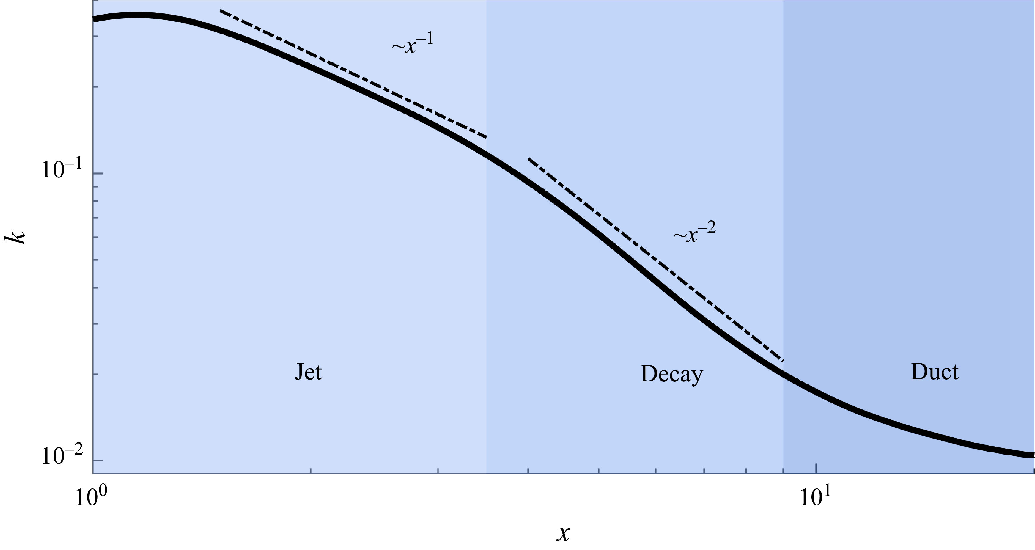
Both jet and decay regions exhibit power-law decreases of the kinetic energy (figure 5). This further supports the analogies to a planar jet and homogeneous decaying turbulence in these regions, which will be studied in detail in §§ 3.1 and 3.2, respectively. The subsequent relaxation toward a duct flow is briefly discussed in § 3.3.
TKE,
 $k$
, averaged over the cross-section along the outlet at
 $\textit{Re}=2000$
. Different flow regions are depicted by different shades of blue.

Cross-sectional colour maps of (a)
 $k$
, (b)
 $P_{k}$
, (c)
 $\langle \theta \rangle$
and (d)
 $\langle \theta ^{\prime 2}\rangle$
for
 $\textit{Re}=2000$
at
 $x=2$
.

3.1. Jet-like flow
In figure 6, we show colour maps of TKE
 $k$
, production
 $P_{k}$
and scalar average and variance at
 $x=2$
. Owing to the left–right and up–down mirror symmetries of the mean turbulent flow, averages were taken over the four quadrants. The laminar inflowing streams are quasi-parabolic and thus carry most of the kinetic energy near the centreline. At the junction, where the flow transitions to turbulence, the vertical velocity profile flattens and as a consequence of the momentum redistribution strong shear layers with high values of
 $k$
and
 $P_{k}$
arise near the vertical walls. However, these do not contribute much to mixing (figure 6
c) because they are located away from the centre. Additionally, elevated values of
 $P_k$
are observed near the centre due to the collision of the inlet streams forming the jet. The resulting jet turbulence feeds the incipient mixing layer, and enhances mixing, as reflected in the scalar variance (figure 6
d).
In figure 7(a), streamwise velocity profiles are shown at several locations along the jet region. To enable comparison with a planar jet, the mean velocity for
 $y \geqslant 0.5$
was first evaluated and subtracted from the velocity profiles. The jet half-width
 $y_{1/2}$
was then determined from these mean-subtracted profiles following the standard approach for co-flow jets (Gaskin & Wood Reference Gaskin and Wood2001; Habli et al. Reference Habli, Mahjoub Saïd, Le Palec and Bournot2014). In jet flows, velocity profiles are typically normalised by the centreline velocity (
 $U_{c}$
) to assess self-similarity behaviour, while the transverse coordinate
 $y$
is scaled either by the jet half-width
 $y_{1/2}$
, as
 $\zeta =y/y_{1/2}$
, or by the axial distance from the jet origin
 $(x_{0})$
, as
 $\eta =y/(x-x_{0})$
. In planar jets, the spreading rate is linear,
 ${{\rm d}y_{1/2}}/{{\rm d}x}=S$
, where
 $S\approx 0.1$
(Pope Reference Pope2000).
(a) Velocity, (b) normalised velocity, (c)
 $P_{k}$
and (d) normalised
 $P_{k}$
profiles at
 $\textit{Re}=2000$
and several positions along the jet region. The dashed line jet profiles in (b) and (d) are from Gutmark & Wygnanski (Reference Gutmark and Wygnanski1976) and Soligo et al. (Reference Soligo, Chiarini and Rosti2025), respectively.

Figure 7. Long description
Panel A: A line graph shows the velocity (U) along the y-axis ranging from 0 to 2, with different colored lines representing various x-values (1.5, 2, 2.5, 3). The x-axis ranges from 0 to 1. Panel B: Another line graph displays normalized velocity (U/Uc) along the y-axis from 0 to 1, with the x-axis ranging from 0 to 2.5. Different colored lines represent various x-values, and a dashed line represents data from Soligo. Panel C: A line graph shows normalized profiles (Pk) along the y-axis from 0 to 0.6, with the x-axis ranging from 0 to 1. Different colored lines represent various x-values. Panel D: A line graph displays normalized profiles (Pk/(Uc^3/y1/2)) along the y-axis from 0 to 20x10^-3, with the x-axis ranging from 0 to 2.5. Different colored lines represent various x-values, and a dashed line represents data from Gutmark.
Using the resulting scaling
 $\eta =0.1\zeta$
within the jet region, the velocity profiles collapse reasonably well onto the theoretical planar-jet profile up to
 $x\leqslant 3$
(figure 7
b). The normalised production
 $P_{k}$
profiles are shown in figure 7(d), where the dashed line represents the benchmark data from Gutmark & Wygnanski (Reference Gutmark and Wygnanski1976) for a planar jet at
 $\textit{Re}=3\times 10^4$
. The closest agreement with their data occurs at
 $x=2.5$
. Nevertheless, it is evident that the self-similarity observed in the velocity profiles is weaker in the production curves. We attribute this discrepancy to the fact that planar jets at
 $\textit{Re}=2000$
fall within the transitional regime. Specifically, Suresh et al. (Reference Suresh, Srinivasan, Sundararajan and Das2008) reported that full self-similar behaviour in planar-jet flows is first reached at
 $\textit{Re} \gt 4000$
. In the transitional regime, the flow is dominated by large coherent structures, and the mean velocity field attains self-similarity much earlier than the higher-order statistics (Suresh et al. Reference Suresh, Srinivasan, Sundararajan and Das2008). Accordingly, we observe a good collapse of the velocity profiles, but a weaker self-similar behaviour in the production profiles.
(a) Reynolds shear stress, (b) streamwise, (c) horizontal and (d) vertical velocity fluctuations at
 $\textit{Re}=2000$
. The dotted and dashed lines are from Gutmark & Wygnanski (Reference Gutmark and Wygnanski1976) and Stanley et al. (Reference Stanley, Sarkar and Mellado2002), respectively.

Figure 8. Long description
Four line graphs illustrate different aspects of velocity and stress fluctuations in a fluid dynamics simulation. Panel A: The line graph shows the Reynolds shear stress (u’w’/Uc^2) against the variable ζ. The graph includes multiple lines representing different values of x (1.5, 2, 2.5, 3) and comparisons with Gutmark and Stanley data. Panel B: The line graph displays the streamwise velocity fluctuations (u’/Uc) against ζ, with lines for different x values and comparisons with Gutmark and Stanley data. Panel C: The line graph presents the horizontal velocity fluctuations (v’/Uc) against ζ, with lines for different x values and comparisons with Gutmark and Stanley data. Panel D: The line graph shows the vertical velocity fluctuations (w’/Uc) against ζ, with lines for different x values and comparisons with Gutmark and Stanley data. Each panel includes dotted and dashed lines representing data from Gutmark & Wygnanski (1976) and Stanley et al. (2002), respectively.
Reynolds shear stress and velocity-fluctuation profiles are shown in figure 8(a–d) at four streamwise locations. Planar-jet measurements are included as reference (Gutmark & Wygnanski Reference Gutmark and Wygnanski1976; Stanley et al. Reference Stanley, Sarkar and Mellado2002). In the central part of the outlet, the Reynolds shear stress and the fluctuations computed from our data exhibit similar profiles and magnitude as the planar-jet data. However, the agreement deteriorates toward the outer part of the cross-section. The difference is particularly pronounced in figure 8(d). Here, the fluctuation level in the T-mixer increases toward the outer region, whereas it decreases in the planar-jet measurements. This difference arises due to the fundamentally different flow configurations. A planar jet develops surrounded by a quiescent ambient fluid, leading to a progressive decay of the velocity fluctuations outside the shear layer. This decay in turbulence intensity is reflected in the turbulent production profile. The T-mixer outlet, by contrast, is a confined, wall-bounded flow in which the outer part of the cross-section is also turbulent. Furthermore, the finite distance between the developing shear layer and the sidewalls and the three-dimensional mean flow generated at the T-junction, modify the local strain field and the redistribution of TKE among the velocity components. The planar-jet analogy therefore is limited to the free shear layer in the central region of the outlet channel. The deviations in the outer region arise due to confinement effects, the turbulent flow alongside the jet and three-dimensionality.
Same as figure 7 but at
 $x=2.5$
and several
 $\textit{Re}$
.

The velocity and production profiles for all
 $\textit{Re}$
investigated in this work are plotted at
 $x=2.5$
in figure 9. As expected, in all cases the velocity profiles exhibit the self-similar behaviour characteristic of planar jets, whereas the production profiles increasingly depart from the self-similar limit as
 $\textit{Re}$
decreases.
Vortex structures defined by iso-surfaces of
 $Q$
criterion (Hunt et al. Reference Hunt, Wray and Moin1988) at 95 % level in the jet region at
 $\textit{Re}=2000$
: (a) three-dimensional view and (b) top view. The colouring is based on the streamwise direction.

Figure 10. Long description
Panel A: A 3D scatter plot shows vortex structures defined by iso-surfaces of a criterion at a 95 percent level in the jet region. The plot includes three axes labeled x, y, and z. The structures are color-coded based on the streamwise direction, transitioning from red to blue. Panel B: A top view of the same vortex structures is presented as a 2D scatter plot. The axes are labeled x and y, with the z-axis omitted. The structures are similarly color-coded based on the streamwise direction. The dashed lines in Panel B represent jet profiles from external references.
The coherent vortex structures in the jet region are similar to those reported in studies of planar jets (figure 10 a). Specifically, it can be observed that, following the collision of the two inlet streams, pairs of vortical core structures are formed. These are highlighted in figure 10(b) within the black dotted rectangles, similar to those reported for planar jets by Wu et al. (Reference Wu, Sakai, Nagata, Ito, Terashima and Hayase2014) and Soligo et al. (Reference Soligo, Chiarini and Rosti2025). The vortices are initially oriented in the spanwise direction and are densely packed near the collision zone, where strong shear and turbulence production occur. As the flow progresses downstream, the two vortical cores elongate in the streamwise direction. In the merger region, indicated in figure 10(b) with a blue rectangle, the vortical pairs interact and combine into more organised coherent structures in the flow direction.
3.2. Decay region
As figure 6 but at
 $x=6$
.

At
 $x=6$
the average streamwise velocity profiles are flat (figure 4) and the kinetic energy has diffused across the entire cross-section (figure 11
a), indicating that the jet has fully spread to the walls and the flow state is nearly homogeneously turbulent. The magnitude of
 $k$
here is an order of magnitude lower than at
 $x=2$
, whereas its maximum value remains near the top and bottom walls. The production is also an order of magnitude lower and is strongly confined to near-wall layers (figure 11
b). The scalar field exhibits a distinctly different distribution. The averaged concentration features a smooth gradient in the spanwise direction from the bulk toward the walls, corresponding to a transition from fully mixed to largely unmixed inlet streams (figure 11
c). In the wall-normal direction, the mixing state is homogeneous. The scalar variance is roughly an order of magnitude lower than at
 $x=2$
and exhibits a similar spanwise distribution as the scalar average, except for thin low-variance layers along the walls (figure 11
d).
(a) Evolution of the cross-sectionally averaged kinetic energy
 $k$
, (b) dissipation
 $\varepsilon _{k}$
and (c) scalar variance
 $\theta ^\prime$
along the outlet at various
 $\textit{Re}$
. The inset in (a) shows
 $v'_{\textit{rms}}/u'_{\textit{rms}}$
(green) and
 $w'_{\textit{rms}}/u'_{\textit{rms}}$
(black) along the centreline for
 $\textit{Re}=2000$
. The inset in (b) shows
 $c_{\varepsilon }=\varepsilon \, k^{-3/2}$
along the centreline.

Figure 12. Long description
Three line graphs depict the evolution of kinetic energy, dissipation, and scalar variance along the outlet at various Reynolds numbers. Panel A: The line graph shows the evolution of the cross-sectionally averaged kinetic energy along the outlet at various Reynolds numbers. The x-axis represents the distance along the outlet (x) in logarithmic scale, and the y-axis represents the kinetic energy (k) in logarithmic scale. The inset shows the ratio of root mean square velocity to mean velocity along the centerline for a specific Reynolds number. Panel B: The line graph shows the evolution of dissipation along the outlet at various Reynolds numbers. The x-axis represents the distance along the outlet (x) in logarithmic scale, and the y-axis represents the dissipation (εk) in logarithmic scale. The inset shows the scaled dissipation along the centerline. Panel C: The line graph shows the evolution of scalar variance along the outlet at various Reynolds numbers. The x-axis represents the distance along the outlet (x) in logarithmic scale, and the y-axis represents the scalar variance (〈θ²〉) in logarithmic scale. Different colors represent different Reynolds numbers: yellow for Re = 700, orange for Re = 1000, purple for Re = 1500, and blue for Re = 2000. The graphs show trends and patterns of how these quantities evolve along the outlet channel.
The general picture remains nearly unchanged along the decay region, while the magnitudes of
 $k$
,
 $P_k$
, the spanwise gradient of
 $\langle \theta \rangle$
and
 $\langle \theta ^{\prime 2} \rangle$
decrease monotonically. Specifically, we show in figure 12(a) that the cross-sectionally averaged TKE decreases as a power law with exponent
 $-2$
at all
 $\textit{Re}$
investigated. As shown in the inset, the flow conditions are nearly isotropic near the centreline, where
 $v'_{\textit{rms}}/u'_{\textit{rms}} \approx w'_{\textit{rms}}/u'_{\textit{rms}} \approx 1$
. The dissipation rate also exhibits a power-law decay, but with an exponent of
 $-3$
(figure 12
b). As shown in the inset of figure 12(b),
 $\varepsilon \ k^{-3/2}$
becomes approximately constant in the decay region and approaches unity as
 $\textit{Re}$
increases, indicating the persistence of fully developed turbulent flow in the decay region. In the (approximately) isotropic region of the outlet, kinetic energy expected to decay as
 \begin{equation} \frac {{\rm d}k}{{\rm d}x}=-\varepsilon , \end{equation}
where the dissipation rate is modelled as
 $\varepsilon = c k^{3/2}/l$
, and
 $l$
is the integral length scale. In a confined flow,
 $l$
is the size of the domain. Substituting this estimate into (3.1) and solving for
 $k$
yields a power-law decay of the form
 $k(x)\sim x^{-2}$
and
 $\varepsilon (x)\sim x^{-3}$
, which is consistent with the decay exponents observed in our DNS. Additionally, the observed decay exponents agree with the values reported by Stalp et al. (Reference Stalp, Skrbek and Donnelly1999) and Touil et al. (Reference Touil, Bertoglio and Shao2002) for turbulence decay in bounded domains, which are significantly higher in magnitude than those reported for homogeneous isotropic turbulence (Panickacheril et al. Reference Panickacheril, Donzis and Sreenivasan2022). This is consistent with the fact that in the decay region of the T-mixer production is confined to the near-wall layers.
The evolution of the scalar variance along the outlet is shown in figure 12(c). At the junction, the two streams are initially largely unmixed and begin to mix in the jet region, leading to an increase in the scalar variance. Meanwhile, the turbulence intensity increases and contributes to decreasing the variance. This leads to a maximum in the variance, which is achieved earlier, the more turbulent the flow is (i.e. at higher
 $\textit{Re}$
). Subsequently, the variance decays monotonically. In the decay region, it eventually follows a power-law decay with an exponent of approximately
 $-10/7$
. This is consistent with the scalar-variance decay reported for homogeneous isotropic turbulence by Chasnov (Reference Chasnov1994) and Lee et al. (Reference Lee, Benaissa, Djenidi, Lavoie and Antonia2012), and clearly different from the exponent for decay in bounded domains (
 $-3.25$
) reported by Lamaison et al. (Reference Lamaison, Bos, Shao and Bertoglio2007). We attribute this to the fact that mixing is initially localised in the vertical mid-plane of the channel and slowly progresses toward the sidewalls (compare figures 6
d and 11
d). Even at
 $x=6$
, the scalar variance remains confined to the central region, where the flow is approximately homogeneous and isotropic.
3.3. Relaxation to duct flow
As in figure 10 for the decay region.

Along the decay region, the turbulent structures become progressively less intense and grow in size (figure 13). From approximately
 $x\gtrsim 9$
onward, they begin to elongate and align in the streamwise direction, marking the beginning of the gradual relaxation toward duct flow. This increase in the anisotropies is quantified in the inset of figure 12(a). The kinetic energy and dissipation rate begin to level off and relax toward turbulent duct-flow values for
 $\textit{Re}=1500$
and
 $2000$
, whereas they continue to fall sharply for
 $\textit{Re}=700$
and
 $1000$
(figure 12
a–b), indicating flow relaminarisation. Note also how, for the latter cases,
 $\varepsilon k^{-3/2}$
increases linearly as a result of the dissipation falling off less sharply than the kinetic energy during the relaminarisation process, whereas for the former it begins to saturates at approximately
 $\varepsilon k^{-3/2} \rightarrow 1.25$
, as in turbulent duct flow, with
 $\varepsilon k^{-3/2} \approx 1.4$
from our computations. However, we stress that the outlet length simulated here (
 $20$
) does not allow for full development of the duct flow. Specifically, at
 $x=18$
and
 $z=0$
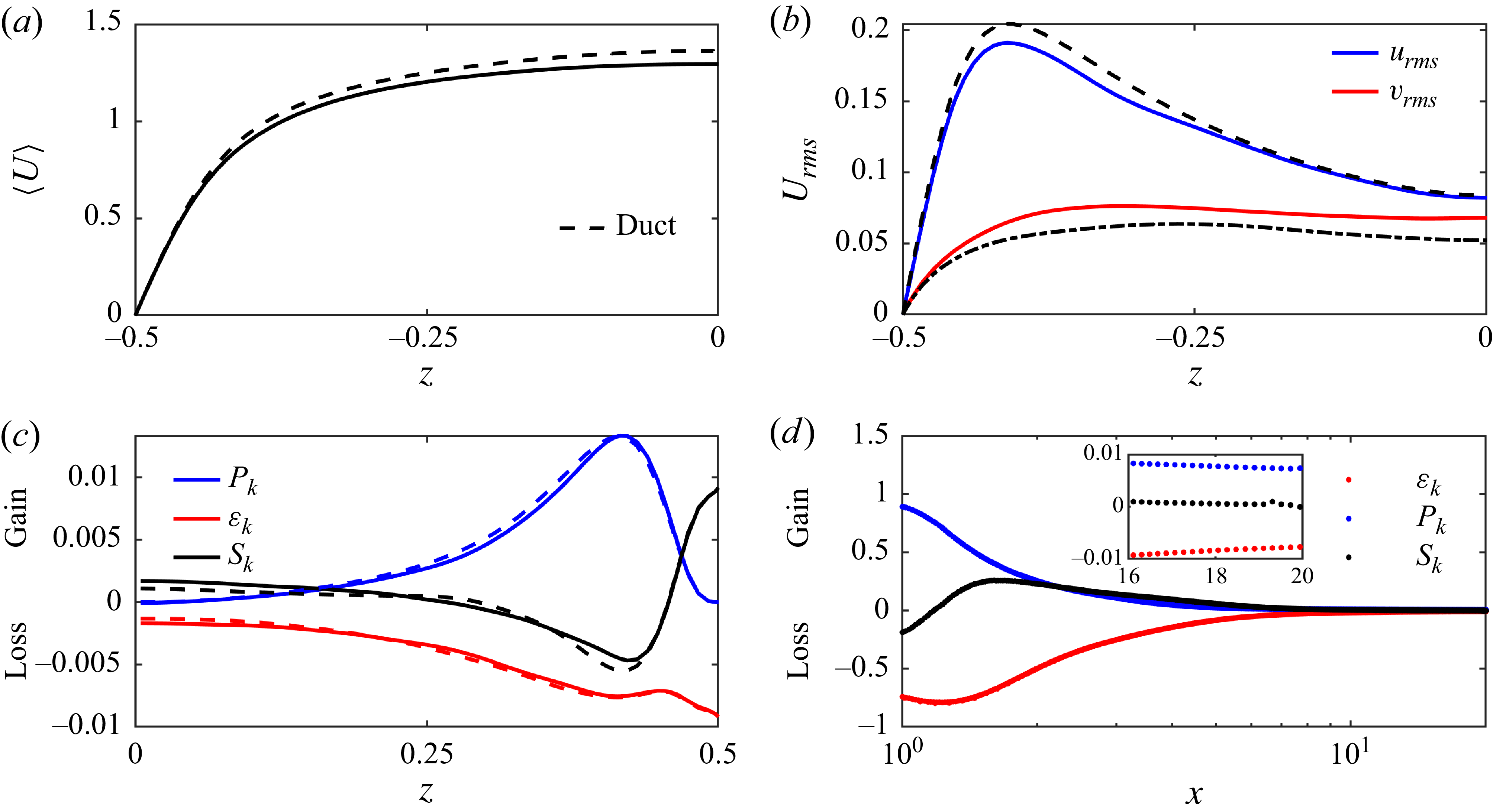
the mean velocity profile is flatter than in duct flow (figure 14
a), and the turbulent intensity is higher (figure 14
b). In figure 14(c), the TKE budget terms at
 $x=18$
and
 $y=0$
are examined. Production
 $P_{k}$
and dissipation
 $\varepsilon _{k}$
are confined to the near-wall regions, and there is a strong flux of kinetic energy, denoted by
 $S_k$
, from the wall toward the bulk. The dashed curves correspond to the reference duct data and indicate that, while the flow is converging and relaxing toward the duct-flow condition, residual turbulence persists and a fully developed duct-flow state has not yet been attained. Finally, we show in figure 14(d) the cross-sectionally integrated TKE budget terms along the outlet. Throughout the jet region there is a strong downstream flux of kinetic energy, which weakens but persists throughout the decay and relaxation regions.
Streamwise velocity profile (a), r.m.s. velocities (b) and production
 $P_{k}$
,
 $\varepsilon _{k}$
and sum of TKE fluxes
 $S_{k}$
along the wall-normal direction (
 $y=0$
and
 $x=18$
) (c). The dashed line represents the rectangular duct data with aspect ratio of
 $2$
at
 $\textit{Re}=2000$
. (d) Cross-sectionally integrated
 $P_{k}$
,
 $\varepsilon _{k}$
and
 $S_{k}$
along the outlet.

Figure 14. Long description
Panel A: A line graph shows the streamwise velocity profile with the horizontal axis labeled as z and the vertical axis labeled as <U>. The graph includes a dashed line representing the rectangular duct data. Panel B: A line graph displays the root mean square (r.m.s.) velocities with the horizontal axis labeled as z and the vertical axis labeled as Urms. The graph includes two lines, one for urms in blue and another for vrms in red, along with a dashed line representing the rectangular duct data. Panel C: A line graph illustrates the production (Pk), dissipation rate (ek), and sum of TKE fluxes along the wall-normal direction (Sk) with the horizontal axis labeled as z and the vertical axis labeled as Gain and Loss. The graph includes three lines, one for Pk in blue, another for ek in red, and a third for Sk in black, along with dashed lines representing the rectangular duct data. Panel D: A line graph shows the cross-sectionally integrated Pk, ek, and Sk along the outlet with the horizontal axis labeled as x and the vertical axis labeled as Gain and Loss. The graph includes three lines, one for Pk in blue, another for ek in red, and a third for Sk in black, along with an inset showing detailed behavior for specific values.
(a) Cross-sectional colour map of mean velocity magnitude and streamlines at
 $x=18$
. (b) Colour map of mean streamwise vorticity at
 $x=18$
.

Streamlines of the mean velocity field and streamwise vorticity are shown in figure 15. The two-vortex pattern in the corner, which is typical of turbulent duct flows, is observed here. The vortex adjacent to the horizontal wall is larger and elongated toward the centre, while the smaller vortex remains closer to the vertical wall. This is as expected for ducts with an aspect ratio of 2, which break the symmetry between the two corner vortices about the corner bisector characteristic of square ducts.
3.4. Mixing process
(a) Spanwise colour map of mean scalar
 $\langle \theta \rangle$
averaged in vertical direction (
 $z$
). (b) Scalar profiles at various streamwise locations, with the corresponding error-function fits shown as solid lines. (c) Computed
 $\delta _{\theta }$
from (3.5) for various
 $\textit{Re}$
. (d) Mixing thickness computed using (3.6) for various
 $\textit{Re}$
. (e) Computed
 $D_{\textit{eff}}$
using (3.8) along the outlet.

Figure 16. Long description
Panel A: A color map showing the spanwise distribution of the mean scalar averaged in the vertical direction. The x-axis ranges from 1 to 20, and the y-axis ranges from -1 to 1. The color gradient indicates scalar values, with a scale bar on the right showing values from 0.2 to 0.8. Panel B: A scatter plot with multiple data series showing scalar profiles at various streamwise locations (x = 1.5, 3, 6, 9, 12, 15). The x-axis ranges from -1 to 1, and the y-axis ranges from 0 to 1. Solid lines represent error-function fits to the data. Panel C: A line graph showing the scalar variance computed for various Reynolds numbers (Re = 700, 1000, 1500, 2000). The x-axis ranges from 1 to 20, and the y-axis ranges from 0.2 to 0.5. Panel D: A line graph showing the mixing thickness computed for various Reynolds numbers. The x-axis ranges from 1 to 20, and the y-axis ranges from 0 to 4. Panel E: A scatter plot showing the effective diffusivity computed along the outlet for various Reynolds numbers. The x-axis ranges from 1.5 to 20, and the y-axis ranges from 0 to 0.3.
Figure 16(a) shows a colour map of the temporally and vertically averaged scalar field,
 $\langle \theta \rangle$
, along the outlet. The thin jet sheet created at the junction expands toward the walls as the two streams gradually mix. The two black lines denote contour levels at 0.4 and 0.6, and are plotted to highlight the expansion of the mixing boundaries. As shown in Appendix A, the following advection-diffusion equation approximately describes the mixing process in the main channel of the T-mixer
 \begin{equation} U\frac {\partial \langle \theta \rangle }{\partial x}=D_{\textit{eff}}\frac {\partial ^2\langle \theta \rangle }{\partial y^2}. \end{equation}
Here,
 $D_{\textit{eff}}=D+D_{t}$
is the effective diffusion coefficient and
 $D_{t}$
is a turbulent eddy diffusivity. For a Heaviside initial condition of the form
 \begin{equation} \langle \theta (x=x_{0},y) \rangle = \begin{cases} 0 & y \lt 0 ,\\ 1 & y \ge 0, \end{cases} \end{equation}
the solution to (3.2) is an error function of the form (Crank Reference Crank1979)
 \begin{equation} \langle \theta (x,y) \rangle =\frac {1}{2}\left[1+\mathrm{erf} \left(\frac {y}{s_{\theta }}\right)\right]\!, \end{equation}
where
 $s_{\theta }=\sqrt {4xD_{\textit{eff}}/U}$
is the slope of the error-function profile and represents the streamwise evolution of the mixing thickness. Although the scalar profiles are not generated from a true Heaviside initial condition in the outlet, they resemble an error-function shape (see figure 16
b). Therefore, an error-function fit to the mean scalar profile can be used to estimate the effective diffusion coefficient,
 $D_{\textit{eff}}$
, along the outlet of the T-mixer. This, in turn, allows us to quantify how each flow region contributes to the overall mixing process. However, this approach has two limitations. First, one must choose the effective origin location
 $x_{0}$
used to evaluate
 $x$
in the expression for
 $s_{\theta }$
. Second, the fitting is sensitive to noise, and the resulting estimates can be quite noisy, masking the underlying physical trend of
 $D_{\textit{eff}}$
along the outlet. An alternative approach is to use scalar integral mixing width
 $\delta _{\theta }$
to compute the effective diffusion coefficient, since it is an integral quantity and therefore less sensitive to noise. For a freely evolving mixing layer, the scalar integral mixing width is expressed as (Blakeley et al. Reference Blakeley, Olson and Riley2022)
 \begin{equation} {\delta }_{\theta }=\int _{-\infty }^{\infty }\langle \theta \rangle (1-\langle \theta \rangle ){\rm d}y. \end{equation}
In the T-mixer the domain is bounded, so the integration limits in the above expression must be replaced by the duct lateral boundaries, i.e. from
 $y=-1$
to
 $y=1$
. For all cases, the integral mixing width
 $\delta _{\theta }$
increases significantly in the jet region and then exhibits a saturating trend toward values around
 $0.5$
at the decay and duct region (see figure 16
c). This is expected, since
 $0.5$
is the maximum value
 $\delta _{\theta }$
can attain based on its definition. These values of
 $\delta _{\theta }$
for each case can then be used to compute the effective diffusion coefficient along the outlet. To compute
 $D_{\textit{eff}}$
from
 $\delta _{\theta }$
, we first need to establish a relation between the two. Substituting (3.4) into the definition of the integral mixing width, (3.5), and integrating over the spanwise direction yields (see Appendix B)
 \begin{equation} \delta _{\theta }=\frac {1}{2}-\frac {1}{2}\mathrm{erf}^2 \left(\frac {1}{s_{\theta }}\right)-\frac {s_{\theta }}{\sqrt {\pi }}\mathrm{erf}\left(\frac {1}{s_{\theta }}\right)e^{(-1/s_{\theta }^2)}+\frac {s_{\theta }}{2}\sqrt {\frac {2}{\pi }}\mathrm{erf}\left(\frac {\sqrt {2}}{s_{\theta }}\right)\!. \end{equation}
Equation (3.6) provides a direct relation between
 $\delta _{\theta }$
and
 $s_{\theta }$
. Using (3.6), the mixing thickness
 $s_{\theta }$
along the outlet can be computed and is plotted in figure 16(d). Since the error function is a self-similar solution of (3.2),
 $s_{\theta }$
evolves downstream according to
 \begin{equation} s_{\theta }(x+\Delta x)=\sqrt {s_{\theta }^2(x)+4\Delta xD_{\textit{eff}}/U}, \end{equation}
where
 $\Delta x$
is the distance between two streamwise locations and
 $D_{\textit{eff}}$
the effective diffusion coefficient for the mixing process between these two locations. This resolves the problem of setting the origin,
 $x_{0}$
, of the Heaviside function. Assuming
 $U=1$
at each cross-section,
 $D_{\textit{eff}}$
can be expressed as
 \begin{equation} D_{\textit{eff}}=\frac {s_{\theta }^2(x+\Delta x)-s_{\theta }^2(x)}{4\Delta x}. \end{equation}
This expression relates
 $D_{\textit{eff}}$
to
 $\delta _{\theta }$
through the mixing thickness
 $s_{\theta }$
; first,
 $s_{\theta }(x)$
is extracted from
 $\delta _{\theta }(x)$
using (3.6), and then the resulting
 $s_{\theta }(x)$
is used in (3.8) to compute
 $D_{\textit{eff}}$
along the outlet.
Figure 16(e) shows the streamwise evolution of the effective diffusion coefficient,
 $D_{\textit{eff}}$
, along the outlet of the T-mixer for different Reynolds numbers calculated with
 $\Delta x=0.5$
. For all cases,
 $D_{\textit{eff}}$
increases sharply immediately downstream of the junction, reflecting the strong enhancement of scalar transport caused by the impingement of the two inlet streams and the formation of the jet region. In this region, intense interface stretching, entrainment and transverse transport produce highly efficient mixing, leading to a rapid increase in the effective diffusivity. The effective diffusion coefficient reaches a maximum near the end of the jet region, indicating the location of strongest mixing activity. Further downstream,
 $D_{\textit{eff}}$
gradually decreases as the influence of the jet weakens, coherent structures decay and scalar gradients become progressively smoother. Nevertheless, the effective diffusivity does not decay to zero, but appears to approach a finite asymptotic value for the two largest Reynolds number cases. This suggests that, for a sufficiently long outlet, these cases would likely approach an asymptotic effective diffusivity associated with fully developed duct-flow dispersion at that specific
 $\textit{Re}$
. The relatively weak variation in the peak location with
 $\textit{Re}$
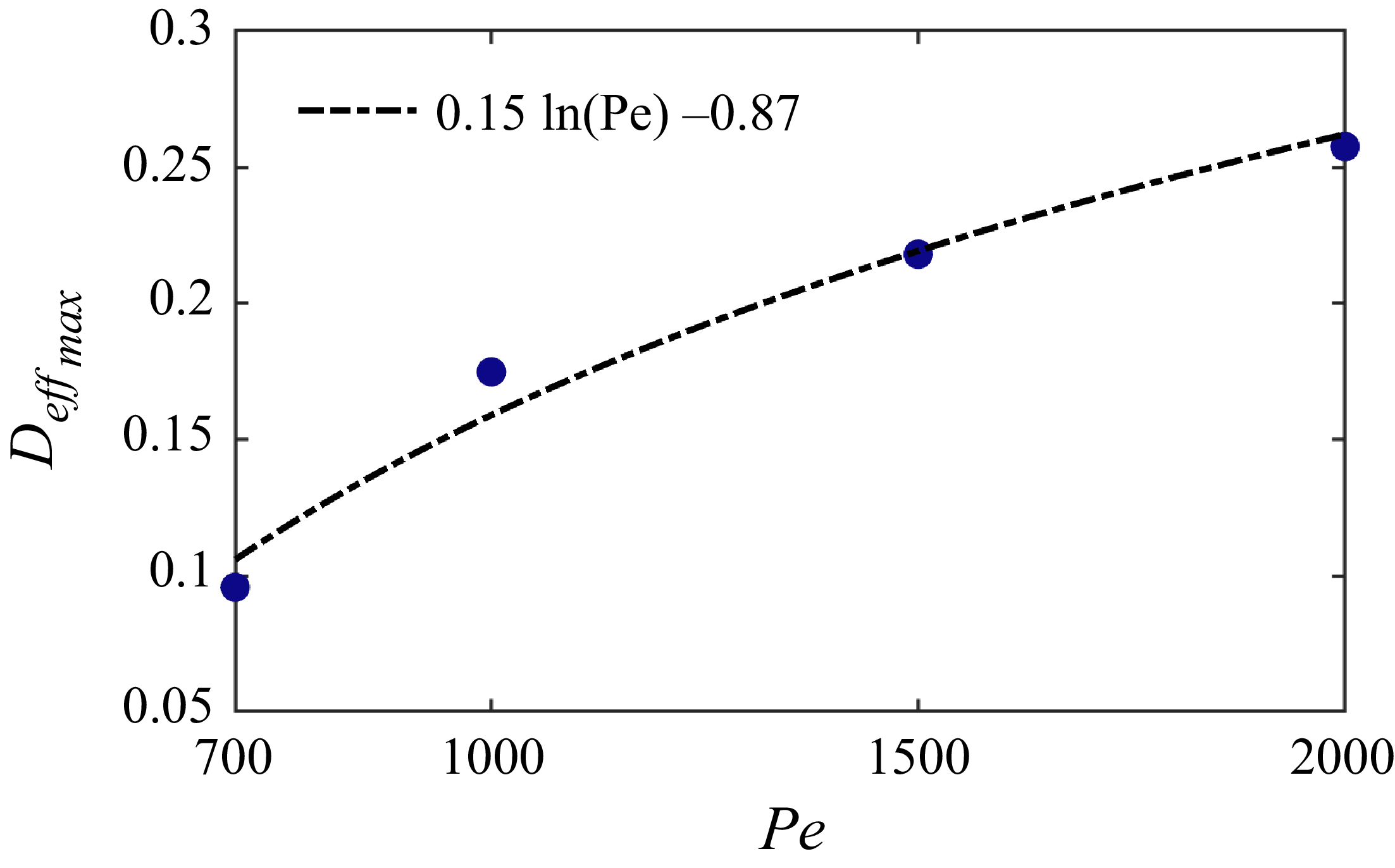
suggests that the streamwise position of maximum mixing is governed primarily by the T-mixer geometry, while the Reynolds number mainly controls the intensity of the mixing process. Figure 17 shows the scaling of the peak value of
 $D_{\textit{eff}}$
with the Péclet number. Within the investigated range of 700
 $\leqslant$
Pe
 $\leqslant$
2000, the data are consistent with a logarithmic trend, although the present dataset is insufficient to distinguish this behaviour from other slowly varying functional forms. Investigating a broader range of Péclet numbers, particularly higher Pe, would be necessary to establish the underlying scaling and determine the asymptotic trend. This apparent logarithmic trend, however, contrasts with classical laminar dispersion, where Taylor (Reference Taylor1953) reported
 $D_{\textit{eff}} \sim {Pe}^2$
, and suggests that, in the T-mixer, increasing
 $\textit{Re}$
or equivalently
 ${Pe}$
, does not significantly enhance mixing (Schikarski et al. Reference Schikarski, Trzenschiok, Peukert and Avila2019).
Scaling of the maximum effective diffusion coefficient with respect to Pe.

4. Conclusion
Turbulence in the outlet of the T-mixer exhibits two distinct regimes analogous to two well-known canonical flows, followed by a slow relaxation toward duct flow. After the collision of the incoming streams at the junction (
 $1.5 \lesssim x \lesssim 3$
), a high-velocity jet forms and displays the typical coherent vortical structures and statistics of a transitional planar jet. This includes a linear decrease of the kinetic energy (Pope Reference Pope2000) and a very good agreement of the streamwise velocity profiles with those of a self-similar planar jet, but less so for the production profiles (Suresh et al. Reference Suresh, Srinivasan, Sundararajan and Das2008). The velocity fluctuations and Reynolds shear stress show good agreement with previous studies (Gutmark & Wygnanski Reference Gutmark and Wygnanski1976; Stanley et al. Reference Stanley, Sarkar and Mellado2002) in the central region, but this agreement deteriorates near the walls as the jet widens and approaches the boundaries. Subsequently (
 $4\lesssim x \lesssim 9$
), a fully developed, nearly homogeneous turbulent state with thin boundary layers at the walls emerges. It is characterised by a power-law decay of kinetic energy and dissipation rate with the exponents typical of decaying turbulence in bounded domains (Stalp et al. Reference Stalp, Skrbek and Donnelly1999; Touil et al. Reference Touil, Bertoglio and Shao2002), i.e.
 $-2$
and
 $-3$
, respectively. By contrast, the decay exponent obtained for the scalar variance (
 $-10/7$
) is in agreement with the values reported for unbounded turbulence Lee et al. (Reference Lee, Benaissa, Djenidi, Lavoie and Antonia2012). We interpret this apparently contradictory behaviour to the fact that the mixing statistics are nearly homogeneous in the wall-normal direction and slowly develop in the spanwise direction from the mid-plane towards the sidewalls without feeling their effect in the decay region. For the laminar inlet boundary conditions employed here, the Reynolds number based on the Taylor microscale reaches a maximum of
 $\textit{Re}_{\lambda }=\sqrt {10k^2/(\varepsilon \nu )}\sim 200$
at the centreline in the junction and for
 $\textit{Re}=2000$
. It decreases down to
 $\textit{Re}_{\lambda }\sim 26$
at the end of the outlet channel, indicating a relaxation toward a fully developed duct flow (
 $\textit{Re}_{\lambda }\sim 24$
), even if this cannot be achieved with the outlet length used here (
 $20d$
).
The need for studying turbulence decay beyond the traditionally considered canonical configurations has been recently emphasised by Verschoof et al. (Reference Verschoof, Huisman, van der Veen, Sun and Lohse2016) and Singh & Prigent (Reference Singh and Prigent2021). Here, we demonstrated that the T-mixer provides a suitable configuration for investigating turbulence decay and jet flows that is accessible in both experiments and simulations, with well-defined reproducible boundary conditions. Although the streamwise profiles of kinetic energy and dissipation are nearly identical at
 $\textit{Re}=2000$
and
 $3000$
(Schikarski et al. Reference Schikarski, Trzenschiok, Peukert and Avila2019), indicating saturation to the asymptotic turbulent state, investigating higher
 $\textit{Re}$
than done here would enable probing the convergence toward a fully developed planar jet and the apparent logarithmic evolution of the effective diffusion with the Péclet number.
Simulations with turbulent inlets merit a separate investigation, as they exhibit a markedly different decay of the kinetic energy and dissipation (Schikarski et al. Reference Schikarski, Trzenschiok, Peukert and Avila2019) after the junction. We argue that this may result from the qualitatively different jet flow that must form when two turbulent (blunted) profiles collide at the junction. Finally, the T-mixer offers the possibility of studying active-scalar mixing in a well-defined, simple setting, which has not been attempted so far despite the relevance of active mixing in chemical engineering (Schikarski et al. Reference Schikarski, Trzenschiok, Avila and Peukert2023). In active-scalar mixing, the scalar affects the velocity field. Therefore, a detailed understanding of the underlying hydrodynamics is necessary in order to separate the influence of the active scalar from the flow dynamics. The results presented here characterise the purely hydrodynamic behaviour of the T-mixer in detail, and thus provide a solid baseline for future studies of active-scalar mixing in T-shaped mixers.
Acknowledgements
The authors would like to thank Dr D.M. Montesdeoca, Dr I. Canoon, P. Keuchel and F. Kranz for their insightful discussions during the revision process.
Funding
This work was supported by the Deutsche Forschungsgemeinschaft (DFG, German Science Foundation) with Grant No. 511099203.
Declaration of interests
The authors report no conflict of interest.
Data availability statement
All data are available in Pangaea under https://doi.pangaea.de/10.1594/PANGAEA.997505.
Appendix A. Approximated advection-diffusion equation in the outlet
We consider the advection-diffusion equation
 \begin{equation} \frac {\partial \theta }{\partial t}+\boldsymbol {u}\boldsymbol{\cdot }\boldsymbol{\nabla }\theta =D\Delta \theta \end{equation}
and, using the Reynolds decomposition, followed by averaging in time, we obtain
 \begin{equation} \langle \boldsymbol{u} \rangle \boldsymbol{\cdot }\boldsymbol{\nabla }\langle \theta \rangle + \left \langle \boldsymbol{u}' \boldsymbol{\cdot }\boldsymbol{\nabla }\theta ' \right \rangle = D {\nabla} ^2 \langle \theta \rangle , \end{equation}
where
 $\langle \boldsymbol {u}\rangle =(\langle u\rangle ,\langle v\rangle ,\langle w\rangle )$
and
 $\boldsymbol {u}'=(u',v',w')$
denote the mean and fluctuating velocity fields. The (A2) can be rearranged as
 \begin{equation} \langle \boldsymbol{u} \rangle \boldsymbol{\cdot }\boldsymbol{\nabla }\langle \theta \rangle = D {\nabla} ^2 \langle \theta \rangle - \boldsymbol{\nabla }\boldsymbol{\cdot }\langle \boldsymbol{u}' \theta ' \rangle , \end{equation}
where
 $\langle \boldsymbol {u}'\theta '\rangle =(\langle u'\theta '\rangle ,\langle v'\theta '\rangle ,\langle w'\theta '\rangle )$
is the turbulent scalar flux vector. We then average the fields in the vertical direction,
 $z$
, which yields
 $\langle w\rangle =0$
. Additionally, since the main flow in the outlet is in the streamwise direction
 $x$
, we can assume
 $\langle v\rangle \approx 0$
. It can also be seen in figure 16(a) that the scalar gradients are much larger in the spanwise direction
 $y$
than the streamwise
 $x$
direction, and the mixing process is mainly a transverse mixing in the
 $y$
direction. Accordingly (A3) reduces to
 \begin{equation} \langle u \rangle \frac {\partial \langle \theta \rangle }{\partial x}=D\frac {\partial ^2\langle \theta \rangle }{\partial y^2}-\frac {\partial \langle v'\theta ' \rangle }{\partial y}. \end{equation}
We use the first-order eddy diffusivity model (Pope Reference Pope2000)
 \begin{equation} \langle v'\theta '\rangle =-D_{t}\frac {\partial \langle \theta \rangle }{\partial y}, \end{equation}
and assume that
 $D_{t}$
does not depend on
 $y$
, and obtain
 \begin{equation} \langle u \rangle \frac {\partial \langle \theta \rangle }{\partial x}=(D+D_{t})\frac {\partial ^2\langle \theta \rangle }{\partial y^2}. \end{equation}
Appendix B. Integral mixing width expression
Starting from the error-function profile (3.4) and inserting it into the definition of integral mixing width (3.5) we get
 \begin{equation} \delta _{\theta }=\frac {1}{2}-\frac {s_{\theta }}{4}\int _{-1/s_{\theta }}^{1/s_{\theta }}\mathrm{erf^2(\lambda )} {\rm d}\lambda, \end{equation}
where
 $\lambda =y/s_{\theta }$
. Since the
 $\mathrm{erf}^2(\lambda )$
is even, we write the integral term as (Korotkov & Korotkov Reference Korotkov and Korotkov2020)
 \begin{equation} I=2\int _{0}^{1/s_{\theta }}\mathrm{erf^2(\lambda )}{\rm d}\lambda =2\lambda \mathrm{erf^2}(\lambda )+\frac {4}{\pi }\mathrm{erf}(\lambda )e^{-\lambda ^2}-\frac {2\sqrt {2}}{\sqrt {\pi }}\mathrm{erf}(\sqrt {2}\lambda ). \end{equation}
Inserting (B2) into (B1), we get
 \begin{equation} \delta _{\theta }=\frac {1}{2}-\frac {1}{2}\mathrm{erf}^2 \left(\frac {1}{s_{\theta }}\right)-\frac {s_{\theta }}{\sqrt {\pi }}\mathrm{erf}\left(\frac {1}{s_{\theta }}\right)e^{(-1/s_{\theta }^2)}+\frac {s_{\theta }}{2}\sqrt {\frac {2}{\pi }}\mathrm{erf}\left(\frac {\sqrt {2}}{s_{\theta }}\right)\!. \end{equation}


 z=0

 N−1=7

 T
 C/T
 T≥200
 C

 Re=2000
 Re=700
 k
 Re=2000

 k
 Pk
 ⟨θ⟩
 ⟨θ′2⟩
 Re=2000
 x=2

 Pk
 Pk
 Re=2000

 Re=2000

 x=2.5
 Re

 Q
 Re=2000

 x=6

 k
 εk
 θ′
 Re
 vrms′/urms′
 wrms′/urms′
 Re=2000
 cε=εk−3/2

 Pk
 εk
 Sk
 y=0
 x=18
 2
 Re=2000
 Pk
 εk
 Sk

 x=18
 x=18

 ⟨θ⟩
 z
 δθ
 Re
 Re
 Deff

 Open access

