1. Introduction
Unsteadiness in flow past bluff bodies or streamlined bodies at large angles of attack, characterized by large-scale vortex shedding in the wake, generates unsteady forces which have the potential to damage the structure and induce unexpected vibrations of bluff bodies (Bearman Reference Bearman1984; Williamson & Govardhan Reference Williamson and Govardhan2004). The mechanism of vortex shedding, a state of saturated self-sustained flow oscillation, has been extensively studied, e.g. in flow past circular cylinders, square cylinders and disks (Williamson Reference Williamson1996; Darekar & Sherwin Reference Darekar and Sherwin2001; Meliga, Chomaz & Sipp Reference Meliga, Chomaz and Sipp2009). It was found that unsteadiness or vortex shedding in the wake of bluff bodies is related to streamwise momentum transfer between the recirculation bubble and the main flow, and a reduction of this transfer reduces the form drag significantly (Stalnov, Fono & Seifert Reference Stalnov, Fono and Seifert2011). Therefore, suppression of wake unsteadiness is expected to not only suppress the force oscillations but also reduce drag acting on bluff bodies.
Vortex shedding control and the related drag reduction techniques may be subdivided into passive and active methods; both have received extensive investigation. The prototypical passive method is to insert splitter plates into the wake in order to reduce near-wake shear layer interaction (Roshko Reference Roshko1954; Bearman Reference Bearman1965; Kwon & Choi Reference Kwon and Choi1996), while a wide variety of other methods have received attention. For example, a small secondary cylinder has been placed on the side of a cylinder to suppress vortex shedding at low Reynolds numbers (Strykowski & Sreenivasan Reference Strykowski and Sreenivasan1990). Spanwise waviness has been adopted in rectangular-cylinder (Bearman & Owen Reference Bearman and Owen1998), circular-cylinder (Owen, Bearman & Szewczyk Reference Owen, Bearman and Szewczyk2001) and square-cylinder (Darekar & Sherwin Reference Darekar and Sherwin2001) wakes to successfully suppress vortex shedding in the wake. The mechanism of suppression was in each case attributed to three-dimensional distortion of the two-dimensional shear layers that otherwise roll up to form vortex streets. Park et al. (Reference Park, Lee, Jeon, Hahn, Kim, Kim, Choi and Choi2006) mounted small tabs to the trailing edges of a blunt body in order to reduce drag. The same control approach was studied numerically by Dipankar, Sengupta & Talla (Reference Dipankar, Sengupta and Talla2007) at Reynolds numbers of
 $\mathit{Re}=63$
, 79 and 150. Wu, Wang & Wu (Reference Wu, Wang and Wu2007) studied the suppression of shedding behind a circular cylinder using travelling waves generated by the flexible surface of the cylinder.
Like the examples given above, passive control of shedding typically involves altering or adding to the geometry of the body, whereas active control typically preserves the geometry and involves adding some kind of forcing. Physically representable control forcing may be generated by various means, e.g. jets/synthetic jets (Glezer & Amitay Reference Glezer and Amitay2002), plasma actuators (Peers, Huang & Luo Reference Peers, Huang and Luo2009) or electromagnetic devices (Zhang, Fan & Chen Reference Zhang, Fan and Chen2010). Often, active control takes the form of controlled blowing into the wake from the surface of the body in order to displace vortex shedding downstream and increase the base pressure (Bearman Reference Bearman1967; Wood Reference Wood1967), and may be either open-loop, as for the base-bleed examples just cited, or closed-loop. Roussopoulos (Reference Roussopoulos1993) used feedback control of wall transpiration to suppress vortex shedding in the wake of a cylinder at a Reynolds number just above the onset of shedding. In wind/water tunnel experiments, he observed that the wake instability in the controlled flow could be delayed to Reynolds numbers 20 % higher than the uncontrolled flow. Gillies (Reference Gillies1998) used multiple sensors and artificial body-force control inputs to suppress the vortex shedding behind a circular cylinder at
 $\mathit{Re}=100$
in a numerical investigation, and demonstrated both that multisensor control is superior to single-sensor control and that it is capable of suppressing shedding when single-sensor control fails. Min & Choi (Reference Min and Choi1999) implemented a suboptimal feedback control strategy targeting the pressure fluctuation on the surface of a cylinder to suppress the vortex shedding in the wake at
 $\mathit{Re}=100$
and 160. The gradient used to update the control was obtained through a Fourier transformation, which is a technique restricted to simple flow geometries, rather than through solving adjoint equations. Homescu, Navon & Li (Reference Homescu, Navon and Li2002) studied the suppression of shedding in the wake of a cylinder by controlling the time-dependent rotating speed of the cylinder at
 $\mathit{Re}=60{-}1000$
. Li et al. (Reference Li, Navon, Hussaini and Le Dimet2003) minimized the difference of the velocity field and that of a steady laminar flow and achieved suppression of vortex shedding in flow past a cylinder at
 $\mathit{Re}\leqslant 110$
by using coarsely distributed wall blowing. Kim & Choi (Reference Kim and Choi2005) imposed spanwise varying blowing/suction on the surface of a cylinder to trigger spanwise phase mismatch of vortex shedding and thus to reduce drag. Shtendel & Seifert (Reference Shtendel and Seifert2014) adopted a combination of blowing and suction around the separation points to delay separation and reduce vortex shedding at Reynolds numbers up to
 $250\times 10^{3}$
.
Most of the previous numerical studies dealing with active control of vortex shedding targeted low-Reynolds-number flows (
 $\mathit{Re}\leqslant 200$
) and did not concentrate on the optimal or most effective control of vortex shedding, which is the goal of the current work. For optimal control of shedding, a sensitivity approach, i.e. one that is optimal in the linear sense, has been previously proposed by Marquet, Sipp & Jacquin (Reference Marquet, Sipp and Jacquin2008) and Marquet & Sipp (Reference Marquet, Sipp, Schlatter and Henningson2010). That approach targets the origin of vortex shedding – asymptotic growth of perturbations based on a steady unstable (base) flow – by calculating the sensitivity of instability with respect to external forcing and using the sensitivity as control to stabilize the flow. The technique was successfully applied in global stabilization and suppression of vortex shedding by using external forcing in the form of a secondary cylinder at
 $47\leqslant \mathit{Re}\leqslant 80$
(Marquet et al.
Reference Marquet, Sipp and Jacquin2008) for flow past a cylinder or
 $\mathit{Re}=100$
for flow around a rotating cylinder (Pralits, Brandt & Giannetti Reference Pralits, Brandt and Giannetti2010), and steady forcing imposed on the surface of a cylinder at
 $\mathit{Re}=47$
(Marquet & Sipp Reference Marquet, Sipp, Schlatter and Henningson2010).
In the literature regarding nonlinear optimal flow control or optimal design, both deterministic (gradient-based) methods and stochastic methods have been widely used. Stochastic methods converge much more slowly than gradient-based methods and would be only suitable when a gradient-based method is unrealistically demanding in a computational sense and the requirement on accuracy is not too harsh. In gradient-based methods, control parameters are updated along a direction related to the gradient of the objective functional with respect to the control. To calculate the gradient, the governing equations, usually the Navier–Stokes (NS) or linearized NS equations, together with their adjoint equations are integrated in time. This gradient can be interpreted as the sensitivity of the control objective with respect to the control forcing, and can be considered as the linearly optimal control when the control magnitude is small enough, as discussed above. If the governing equations are nonlinear or the time integration of the primitive variables is involved in the cost functional, the full temporal development trajectory of the velocity components has to be saved for solving the adjoint. The adjoint equations can be dealt with in either discrete or continuous form (Giles & Pierce Reference Giles and Pierce2000). Discrete adjoint methods have been implemented in design optimizations by Homescu et al. (Reference Homescu, Navon and Li2002), Nielsen, Diskin & Yamaleev (Reference Nielsen, Diskin and Yamaleev2010) and Nielsen & Jones (Reference Nielsen and Jones2011). However, the discrete adjoint equations are dependent on the discretization method and the grid and therefore cannot be generalized easily. Recently, a continuous adjoint method to calculate the optimal boundary perturbation that induces largest gain was introduced (Mao, Blackburn & Sherwin Reference Mao, Blackburn and Sherwin2012), and that method can be developed into the optimal control method used in the present work by redefining the optimal boundary perturbation as the most effective control.
In the following, we detail the optimal control algorithms in § 2, present the discretization and convergence in § 3 and then apply the method to optimal control of vortex shedding in flow past a circular cylinder in § 4 before drawing conclusions in § 5. As we shall demonstrate, the generality of the optimal control method we have adopted potentially allows one to identify strategies that might not otherwise be realized, as observed in the following study at higher Reynolds numbers. Unlike the approach of Marquet & Sipp (Reference Marquet, Sipp, Schlatter and Henningson2010), which is based upon eigenanalysis of local flow states and so readily provides a physical insight through the eigenanalysis, the generality of our approach may potentially initially obscure the nature of the underlying physics. Nevertheless, one can still analyse the physics and stability of the resulting optimally controlled flow, as we have done in the following study.
2. Methodology
In the following, all velocities are taken to be normalized by the free-stream flow speed and all lengths are normalized by the cylinder diameter. Hence, also, time is normalized by the ratio of cylinder diameter to free-stream speed.
2.1. Modelling the unsteadiness
To simplify notation, we introduce scalar products
 $$\begin{eqnarray}(\boldsymbol{a},\boldsymbol{b})=\int _{{\it\Omega}}\boldsymbol{a}\boldsymbol{\cdot }\boldsymbol{b}\,\text{d}V,\quad \langle \boldsymbol{c},\boldsymbol{d}\rangle ={\it\tau}^{-1}\int _{0}^{{\it\tau}}(\boldsymbol{c},\boldsymbol{d})\,\text{d}t,\quad [\boldsymbol{e},\boldsymbol{f}]=\int _{\partial {\it\Omega}_{c}}\boldsymbol{e}\boldsymbol{\cdot }\boldsymbol{f}\,\text{d}S,\end{eqnarray}$$
where
 ${\it\Omega}$
represents the spatial domain,
 $\partial {\it\Omega}_{c}$
denotes the control boundary, referring to the boundary segment where the control is imposed,
 $t$
is time,
 ${\it\tau}$
is a final time,
 $\boldsymbol{a}$
and
 $\boldsymbol{b}$
are vector fields defined on the spatial domain
 ${\it\Omega}$
,
 $\boldsymbol{c}$
and
 $\boldsymbol{d}$
are defined on the spatial domain
 ${\it\Omega}$
and time domain
 $[0,{\it\tau}]$
, and
 $\boldsymbol{e}$
and
 $\boldsymbol{f}$
are defined on the control boundary
 $\partial {\it\Omega}_{c}$
.
In an initial test of the control effects of boundary perturbations, it is observed that the optimal control is concentrated on the wall-normal component. Therefore, in the following, we consider Dirichlet-type boundary-normal velocity perturbations as the control, denoted as
 $\boldsymbol{u}_{c}(\boldsymbol{x},t)$
, where
 $\boldsymbol{x}$
represents the coordinate of the control boundary. To reduce the dimension of
 $\boldsymbol{u}_{c}(\boldsymbol{x},t)$
after temporal–spatial discretization, we decompose the temporal and spatial dependence as
 $$\begin{eqnarray}\boldsymbol{u}_{c}(\boldsymbol{x},t)=u_{n}(\boldsymbol{x})f(t,{\it\omega})\boldsymbol{n},\end{eqnarray}$$
where
 $u_{n}(\boldsymbol{x})$
is the spatial dependence of the perturbation on the wall-normal direction to be optimized,
 $\boldsymbol{n}$
is the outward-pointing unit normal vector on the boundary and
 $f(t,{\it\omega})$
is a prescribed temporal-dependence function. In this work, we adopt a temporal function
 $$\begin{eqnarray}f(t,{\it\omega})=[1-\exp (-t^{2})]\cos ({\it\omega}t),\end{eqnarray}$$
where the first term on the right ensures
 $\boldsymbol{u}_{c}(\boldsymbol{x},0)=0$
so as to avoid temporal discontinuity in the numerical simulation at
 $t=0$
. When the final time
 ${\it\tau}$
is large enough,
 ${\it\omega}$
becomes the frequency of the control perturbation.
The flow field can be decomposed as the sum of an uncontrolled base flow and a perturbation flow induced by the control, i.e.
 $(\hat{\boldsymbol{u}},\hat{p})=(\boldsymbol{U},P)+(\boldsymbol{u},p)$
, where
 $\hat{\boldsymbol{u}}$
,
 $\boldsymbol{U}$
and
 $\boldsymbol{u}$
are respectively the total velocity, uncontrolled velocity and perturbation velocity, while
 $\hat{p}$
,
 $P$
and
 $p$
are the total pressure, uncontrolled pressure and perturbation pressure. Then, we substitute this decomposition into the NS equation to reach
 $$\begin{eqnarray}\partial _{t}\boldsymbol{u}+\boldsymbol{u}\boldsymbol{\cdot }\boldsymbol{{\rm\nabla}}\boldsymbol{u}+\boldsymbol{U}\boldsymbol{\cdot }\boldsymbol{{\rm\nabla}}\boldsymbol{u}+\boldsymbol{u}\boldsymbol{\cdot }\boldsymbol{{\rm\nabla}}\boldsymbol{U}+\boldsymbol{{\rm\nabla}}p-\mathit{Re}^{-1}\boldsymbol{{\rm\nabla}}^{2}\boldsymbol{u}=0,\quad \text{with}~\boldsymbol{{\rm\nabla}}\boldsymbol{\cdot }\boldsymbol{u}=0.\end{eqnarray}$$
In the following, this equation is written in a compact form as
 $$\begin{eqnarray}\partial _{t}\boldsymbol{u}-L(\boldsymbol{u})+N(\boldsymbol{u})=0,\end{eqnarray}$$
where
 $N(\boldsymbol{u})=\boldsymbol{u}\boldsymbol{\cdot }\boldsymbol{{\rm\nabla}}\boldsymbol{u}$
denotes the nonlinear convection term and
 $L(\boldsymbol{u})$
represents the pressure and viscous terms as well as the divergence-free condition, which are linear. In the following this equation will be referred to as the decomposed NS equation.
Since the control perturbation is imposed at
 $t=0$
, the initial condition of perturbation
 $\boldsymbol{u}$
is set to zero. This initial condition is compatible with the control perturbation defined in (2.2).
On the inflow and far-field boundaries, zero Dirichlet and computed Neumann conditions are adopted for
 $\boldsymbol{u}$
and
 $p$
(Blackburn & Sherwin Reference Blackburn and Sherwin2004) respectively; on the outflow boundary,
 $\boldsymbol{{\rm\nabla}}_{\boldsymbol{n}}\boldsymbol{u}=0$
and
 $p=0$
are imposed; on the control boundary, the Dirichlet boundary condition and computed Neumann condition are implemented for
 $\boldsymbol{u}$
and
 $p$
respectively.
For convenience, we define an operator
 $\mathscr{N}$
corresponding to the action of evolving
 $u_{n}(\boldsymbol{x})$
to
 $\boldsymbol{u}(t)$
by integrating the decomposed NS equation (2.5), i.e.
 $$\begin{eqnarray}\boldsymbol{u}(t)=\mathscr{N}(u_{n}).\end{eqnarray}$$
The unsteadiness of the flow field over the time horizon
 $[0,{\it\tau}]$
can be modelled as the fluctuation energy
 $$\begin{eqnarray}A(\boldsymbol{u})=\langle W\hat{\boldsymbol{u}},W\hat{\boldsymbol{u}}\rangle -(W\hat{\boldsymbol{u}}_{a},W\hat{\boldsymbol{u}}_{a}),\end{eqnarray}$$
where
 $W$
is a non-negative spatial weight used to filter the unsteadiness in the regions not of interest when we are only concerned about the unsteadiness in a localized region of the computational domain. When the unsteadiness across the whole domain is taken into account uniformly,
 $W(\boldsymbol{x})=1$
. Here,
 $\hat{\boldsymbol{u}}_{a}$
is the averaged velocity, calculated as
 $$\begin{eqnarray}\hat{\boldsymbol{u}}_{a}=\boldsymbol{U}_{a}+\boldsymbol{u}_{a},\quad \text{where}~\boldsymbol{U}_{a}={\it\tau}^{-1}\int _{0}^{{\it\tau}}\boldsymbol{U}\,\text{d}t\quad \text{and}\quad \boldsymbol{u}_{a}={\it\tau}^{-1}\int _{0}^{{\it\tau}}\boldsymbol{u}\,\text{d}t\end{eqnarray}$$
represent the averaged velocities of base flow and perturbation flow respectively. For flow around a cylinder at the relatively low Reynolds number considered in this work, this unsteadiness quantifies the magnitude of vortex shedding, while for a fully turbulent flow at higher Reynolds number, it describes the turbulence intensity.
2.2. Lagrangian functional
Similarly to the methodology established by Mao et al. (Reference Mao, Blackburn and Sherwin2012) to calculate the optimal boundary perturbation that results in maximum energy in the domain over a finite time horizon, a Lagrangian functional can be defined as
 $$\begin{eqnarray}\mathscr{L}=A-\langle \boldsymbol{u}^{\ast },\partial _{t}\boldsymbol{u}-L(\boldsymbol{u})+N(\boldsymbol{u})\rangle +{\it\lambda}(E-[u_{n},u_{n}]),\end{eqnarray}$$
where
 $\boldsymbol{u}^{\ast }$
represents the adjoint velocity,
 ${\it\lambda}$
is a Lagrange multiplier and
 $E$
is a prescribed control cost which is equal to the square of the wall transpiration velocity integrated over the controlled surface. Hence, for the circular cylinder, an equivalent root-mean-square (r.m.s.) value of the transpiration velocity may be computed as
 $(E/{\rm\pi})^{1/2}$
. The first term following the equality in (2.9) represents the unsteadiness or the fluctuation energy to be minimized, the second term applies the constraint of the governing equation, which is the decomposed NS equation (2.5), and the third term is the constraint on the control cost or the magnitude of the control perturbation. Various options for the constraint on the magnitude of perturbations have been discussed by Foures, Caulfield & Schmid (Reference Foures, Caulfield and Schmid2012), while the one we adopt reflects the momentum coefficient.
The adjoint variables are calculated from an adjoint equation. To facilitate the derivation of the adjoint equation, we reformulate the Lagrangian functional. Using integration by parts and the divergence theorem (Barkley, Blackburn & Sherwin Reference Barkley, Blackburn and Sherwin2008), we have
 $$\begin{eqnarray}\displaystyle -\langle \boldsymbol{u}^{\ast },\partial _{t}\boldsymbol{u}-L(\boldsymbol{u})\rangle & = & \displaystyle \langle \boldsymbol{u},\partial _{t}\boldsymbol{u}^{\ast }+L^{\ast }(\boldsymbol{u}^{\ast })\rangle -{\it\tau}^{-1}(\boldsymbol{u}_{{\it\tau}},\boldsymbol{u}_{{\it\tau}}^{\ast })\nonumber\\ \displaystyle & & \displaystyle +\,{\it\tau}^{-1}\int _{0}^{{\it\tau}}\int _{\partial {\it\Omega}}\boldsymbol{n}\boldsymbol{\cdot }[-\boldsymbol{U}(\boldsymbol{u}\boldsymbol{\cdot }\boldsymbol{u}^{\ast })+\boldsymbol{u}p^{\ast }-\boldsymbol{u}^{\ast }p\nonumber\\ \displaystyle & & \displaystyle +\,\mathit{Re}^{-1}(\boldsymbol{{\rm\nabla}}\boldsymbol{u}\boldsymbol{\cdot }\boldsymbol{u}^{\ast }-\boldsymbol{{\rm\nabla}}\boldsymbol{u}^{\ast }\boldsymbol{\cdot }\boldsymbol{u})]\,\text{d}S\,\text{d}t,\end{eqnarray}$$
where
 $\partial {\it\Omega}$
represents all the boundaries of the computational domain;
 $\boldsymbol{u}_{{\it\tau}}^{\ast }$
and
 $\boldsymbol{u}_{{\it\tau}}$
are the adjoint and perturbation velocity vector at
 $t={\it\tau}$
respectively;
 $L^{\ast }(\boldsymbol{u}^{\ast })=\boldsymbol{U}\boldsymbol{\cdot }\boldsymbol{{\rm\nabla}}\boldsymbol{u}^{\ast }-\boldsymbol{{\rm\nabla}}\boldsymbol{U}\boldsymbol{\cdot }\boldsymbol{u}^{\ast }-\boldsymbol{{\rm\nabla}}p^{\ast }+\mathit{Re}^{-1}\boldsymbol{{\rm\nabla}}^{2}\boldsymbol{u}^{\ast }$
and
 $\boldsymbol{{\rm\nabla}}\boldsymbol{\cdot }\boldsymbol{u}^{\ast }=0$
. We note that
 $\partial _{t}\boldsymbol{u}^{\ast }+L^{\ast }(\boldsymbol{u}^{\ast })=0$
is the adjoint equation extensively used in investigations of receptivity and non-normality (Hill Reference Hill1995; Giannetti & Luchini Reference Giannetti and Luchini2007; Barkley et al.
Reference Barkley, Blackburn and Sherwin2008). In the derivation of (2.10), the zero initial condition of
 $\boldsymbol{u}$
is implied. Substituting (2.10) into (2.9), we have a reformulated Lagrangian functional
 $$\begin{eqnarray}\displaystyle \mathscr{L} & = & \displaystyle A-\langle \boldsymbol{u}^{\ast },N(\boldsymbol{u})\rangle +{\it\lambda}(E-[u_{n},u_{n}])+\langle \boldsymbol{u},\partial _{t}\boldsymbol{u}^{\ast }+L^{\ast }(\boldsymbol{u}^{\ast })\rangle -{\it\tau}^{-1}(\boldsymbol{u}_{{\it\tau}},\boldsymbol{u}_{{\it\tau}}^{\ast })\nonumber\\ \displaystyle & & \displaystyle +\,{\it\tau}^{-1}\int _{0}^{{\it\tau}}\int _{\partial {\it\Omega}}\boldsymbol{n}\boldsymbol{\cdot }[-\boldsymbol{U}(\boldsymbol{u}\boldsymbol{\cdot }\boldsymbol{u}^{\ast })+\boldsymbol{u}p^{\ast }-\boldsymbol{u}^{\ast }p\nonumber\\ \displaystyle & & \displaystyle +\,\mathit{Re}^{-1}(\boldsymbol{{\rm\nabla}}\boldsymbol{u}\boldsymbol{\cdot }\boldsymbol{u}^{\ast }-\boldsymbol{{\rm\nabla}}\boldsymbol{u}^{\ast }\boldsymbol{\cdot }\boldsymbol{u})]\,\text{d}S\,\text{d}t.\end{eqnarray}$$
As stated above, the adjoint variables are calculated from an adjoint equation, which can be obtained by setting the first variation of the Lagrangian with respect to
 $\boldsymbol{u}$
to zero. On the right-hand side of (2.11), the variation of the first term with respect to the velocity vector
 $\boldsymbol{u}$
is
 $$\begin{eqnarray}{\it\delta}A({\it\delta}\boldsymbol{u})=\langle {\it\delta}\boldsymbol{u},2W^{2}(\boldsymbol{U}+\boldsymbol{u}-\boldsymbol{U}_{a}-\boldsymbol{u}_{a})\rangle ,\end{eqnarray}$$
where we have used the relation
 $(\boldsymbol{u}_{a},\boldsymbol{u}_{a})=\langle \boldsymbol{u}_{a},\boldsymbol{u}\rangle$
and similar manipulations. Next, we consider the variation of the second term with respect to
 $\boldsymbol{u}$
, i.e.
 $$\begin{eqnarray}{\it\delta}\langle \boldsymbol{u}^{\ast },N(\boldsymbol{u})\rangle ({\it\delta}\boldsymbol{u})=\langle {\it\delta}\boldsymbol{u},\boldsymbol{{\rm\nabla}}\boldsymbol{u}\boldsymbol{\cdot }\boldsymbol{u}^{\ast }-\boldsymbol{u}\boldsymbol{\cdot }\boldsymbol{{\rm\nabla}}\boldsymbol{u}^{\ast }\rangle +{\it\tau}^{-1}\int _{0}^{{\it\tau}}\int _{\partial {\it\Omega}}({\it\delta}\boldsymbol{u}\boldsymbol{\cdot }\boldsymbol{u}^{\ast })(\boldsymbol{n}\boldsymbol{\cdot }\boldsymbol{u})\,\text{d}S\,\text{d}t.\end{eqnarray}$$
(For details of this derivation, refer to appendix A.)
Combining (2.11)–(2.13), we have the variation of the Lagrangian with respect to
 $\boldsymbol{u}$
,
 $$\begin{eqnarray}\displaystyle {\it\delta}\mathscr{L}({\it\delta}\boldsymbol{u}) & = & \displaystyle \langle {\it\delta}\boldsymbol{u},\partial _{t}\boldsymbol{u}^{\ast }+L^{\ast }(\boldsymbol{u}^{\ast })-\boldsymbol{{\rm\nabla}}\boldsymbol{u}\boldsymbol{\cdot }\boldsymbol{u}^{\ast }+\boldsymbol{u}\boldsymbol{\cdot }\boldsymbol{{\rm\nabla}}\boldsymbol{u}^{\ast }+2W^{2}(\boldsymbol{U}+\boldsymbol{u}-\boldsymbol{U}_{a}-\boldsymbol{u}_{a})\rangle \nonumber\\ \displaystyle & & \displaystyle -\,{\it\tau}^{-1}({\it\delta}\boldsymbol{u}_{{\it\tau}},\boldsymbol{u}_{{\it\tau}}^{\ast })+{\it\tau}^{-1}\int _{0}^{{\it\tau}}\int _{\partial {\it\Omega}}\boldsymbol{n}\boldsymbol{\cdot }[-(\boldsymbol{U}+\boldsymbol{u})({\it\delta}\boldsymbol{u}\boldsymbol{\cdot }\boldsymbol{u}^{\ast })+{\it\delta}\boldsymbol{u}p^{\ast }-\boldsymbol{u}^{\ast }{\it\delta}p({\it\delta}\boldsymbol{u})\nonumber\\ \displaystyle & & \displaystyle +\,\mathit{Re}^{-1}(\boldsymbol{{\rm\nabla}}{\it\delta}\boldsymbol{u}\boldsymbol{\cdot }\boldsymbol{u}^{\ast }-\boldsymbol{{\rm\nabla}}\boldsymbol{u}^{\ast }\boldsymbol{\cdot }{\it\delta}\boldsymbol{u})]\,\text{d}S\,\text{d}t,\end{eqnarray}$$
where
 ${\it\delta}p({\it\delta}\boldsymbol{u})$
is the variation of
 $p$
induced by the variation of
 $\boldsymbol{u}$
. In this derivation,
 $\boldsymbol{u}$
,
 $\boldsymbol{u}^{\ast }$
and
 $u_{n}$
are considered as independent variables. Setting this variation to zero, we obtain the adjoint equation, its initial condition and boundary conditions.
From the first term on the right-hand side of (2.14) we have the adjoint equation:
 $$\begin{eqnarray}\partial _{t}\boldsymbol{u}^{\ast }+L^{\ast }(\boldsymbol{u}^{\ast })-\boldsymbol{{\rm\nabla}}\boldsymbol{u}\boldsymbol{\cdot }\boldsymbol{u}^{\ast }+\boldsymbol{u}\boldsymbol{\cdot }\boldsymbol{{\rm\nabla}}\boldsymbol{u}^{\ast }+2W^{2}(\boldsymbol{U}+\boldsymbol{u}-\boldsymbol{U}_{a}-\boldsymbol{u}_{a})=0.\end{eqnarray}$$
Inspecting the sign of the time derivative term and diffusion term, we see that this equation should be integrated backwards from
 $t={\it\tau}$
to
 $t=0$
. The initial condition
 $\boldsymbol{u}_{{\it\tau}}^{\ast }$
can be obtained from the second term on the right-hand side of (2.14), that is
 $\boldsymbol{u}_{{\it\tau}}^{\ast }=0$
.
The boundary condition of this adjoint equation can be obtained from the last term of (2.14). The combination of adjoint velocity and pressure boundary conditions has to ensure that the integration in the last term of (2.14) over each boundary is zero. On the inflow boundary, control boundary and far-field boundary, the velocity is fixed and therefore
 ${\it\delta}\boldsymbol{u}=0$
. On these three boundaries, zero Dirichlet and computed Neumann conditions are used for adjoint variables
 $\boldsymbol{u}^{\ast }$
and
 $p^{\ast }$
respectively. On the outflow boundary, the boundary conditions for adjoint variables are
 $\mathit{Re}^{-1}\boldsymbol{{\rm\nabla}}_{\boldsymbol{n}}\boldsymbol{u}^{\ast }+\boldsymbol{n}\boldsymbol{\cdot }(\boldsymbol{U}+\boldsymbol{u})\boldsymbol{u}^{\ast }=0$
and
 $p^{\ast }=0$
, where
 $\boldsymbol{{\rm\nabla}}_{\boldsymbol{n}\boldsymbol{u}}^{\ast }=\boldsymbol{n}\boldsymbol{\cdot }\boldsymbol{{\rm\nabla}}\boldsymbol{u}^{\ast }$
(Mao, Blackburn & Sherwin Reference Mao, Blackburn and Sherwin2013). The choices of these boundary conditions ensure that the integration over the boundaries in the last term in (2.14) is zero. It is worth noting that the adjoint velocity outflow boundary condition is dependent on the velocity vector
 $\boldsymbol{u}$
, and so this boundary condition has to be updated (to the latest
 $\boldsymbol{u}$
) at every time step when solving the adjoint equation.
From the last term of (2.11), we have the variation of the Lagrangian with respect to the control perturbation
 $u_{n}$
,
 $$\begin{eqnarray}{\it\delta}\mathscr{L}({\it\delta}u_{n})=[g-2{\it\lambda}u_{n},{\it\delta}u_{n}],\end{eqnarray}$$
where
 $$\begin{eqnarray}g={\it\tau}^{-1}\boldsymbol{n}\boldsymbol{\cdot }\int _{0}^{{\it\tau}}(p^{\ast }\boldsymbol{n}-\mathit{Re}^{-1}\boldsymbol{{\rm\nabla}}_{\boldsymbol{ n}}\boldsymbol{u}^{\ast })f(t,-{\it\omega})\,\text{d}t.\end{eqnarray}$$
Here,
 $f(t,-{\it\omega})$
is the adjoint of
 $f(t,{\it\omega})$
, satisfying
 $[\,f(t,{\it\omega})\boldsymbol{e},\boldsymbol{f}]=[\boldsymbol{e},f(t,-{\it\omega})\boldsymbol{f}]$
, with
 $\boldsymbol{e}$
and
 $\boldsymbol{f}$
representing vectors defined on the control boundary.
From the definition of the gradient of the Lagrangian associated with the Gâteaux differential, the gradient of
 $\mathscr{L}$
with respect to
 $u_{n}$
is
 $$\begin{eqnarray}\boldsymbol{{\rm\nabla}}_{\boldsymbol{u}_{\boldsymbol{n}}}\mathscr{L}=g-2{\it\lambda}u_{n}.\end{eqnarray}$$
In this formulation, both
 $g$
and
 $u_{n}$
are functions defined on the control boundary.
2.3. Nonlinear optimal control
To compute an optimal solution of
 $u_{n}$
, an iterative optimization algorithm is required. For the gradient-based optimization methods, in each iteration, the gradient of the Lagrangian with respect to the control has to be evaluated. From the expression of the gradient in (2.18), we see that the adjoint equation must be solved to calculate
 $g$
and then the gradient. From the adjoint equation and its boundary conditions, we note that the full development history of
 $\boldsymbol{u}$
is required to solve the adjoint variables. Solving the adjoint equation is computationally as intense as solving the decomposed NS equation, but requires much larger memory. To reduce this high requirement on memory, a checkpointing scheme has been proposed by Griewank (Reference Griewank1992). In that scheme, the memory requirement can be significantly reduced but the governing equation (2.5) and the adjoint equation (2.15) have to be restarted at every checkpoint. In the numerical method we presently implement to solve these equations, large-scale matrices need to be generated and installed every time the equation solvers are restarted, and therefore such a checkpointing scheme is inefficient. In the current work, the development history of
 $\boldsymbol{u}$
at every time step is written to file when integrating the decomposed NS equation (2.5) and read into memory at every step with the reversed order when integrating the adjoint equation (2.15).
In the optimization algorithm, a steepest-descent method is used and therefore the search direction is the gradient itself. The control perturbation and perturbation velocity are updated along this direction from iterative step
 $k$
to
 $k+1$
as
 $$\begin{eqnarray}u_{n}^{k+1}=u_{n}^{k}+{\it\alpha}\boldsymbol{{\rm\nabla}}_{\boldsymbol{ u}_{\boldsymbol{n}}}\mathscr{L}^{k}=u_{n}^{k}+{\it\alpha}g^{k}-2{\it\alpha}{\it\lambda}u_{n}^{k},\end{eqnarray}$$
where
 ${\it\alpha}$
is a step length and
 ${\it\lambda}$
can be obtained by imposing the constraint of control cost on
 $u_{n}^{k+1}$
.
Correspondingly, the perturbation velocity at step
 $k+1$
can be obtained as
 $$\begin{eqnarray}\boldsymbol{u}^{k+1}(t)=\mathscr{N}(u_{n}^{k}+{\it\alpha}g^{k}-2{\it\alpha}{\it\lambda}u_{n}^{k}).\end{eqnarray}$$
If the step length
 ${\it\alpha}$
is small enough,
 ${\it\alpha}g^{k}$
and
 $-2{\it\alpha}{\it\lambda}u_{n}^{k}$
are small compared with
 $u_{n}^{k}$
. Therefore, we have
 $$\begin{eqnarray}\boldsymbol{u}_{l}^{k+1}=\boldsymbol{u}^{k}+{\it\alpha}\mathscr{M}_{\boldsymbol{ U}+\boldsymbol{u}}(g^{k})-2{\it\alpha}{\it\lambda}\mathscr{M}_{\boldsymbol{ U}+\boldsymbol{u}}(u_{n}^{k}),\end{eqnarray}$$
where
 $\boldsymbol{u}_{l}^{k+1}$
is the linearized approximation of
 $\boldsymbol{u}^{k+1}$
. Here,
 $\mathscr{M}_{\boldsymbol{U}+\boldsymbol{u}}$
is a linearized approximation to
 $\mathscr{N}$
and
 $\mathscr{M}_{\boldsymbol{U}+\boldsymbol{u}}(g)$
can be obtained by taking
 $gf(t,{\it\omega})\boldsymbol{n}$
as the boundary condition,
 $\boldsymbol{U}+\boldsymbol{u}^{k}$
as the base flow and integrating the linearized NS equation
 $$\begin{eqnarray}\partial _{t}\boldsymbol{u}-L(\boldsymbol{u})=0\end{eqnarray}$$
from
 $t=0$
to
 $t={\it\tau}$
, with the same boundary condition and initial condition as the decomposed NS equation;
 $\mathscr{M}_{\boldsymbol{U}+\boldsymbol{u}}(u_{n}^{k})$
can be obtained similarly.
Substituting (2.21) into (2.7), we see that the unsteadiness
 $A$
can be expressed as a polynomial function of
 ${\it\alpha}$
, and therefore the optimal value of
 ${\it\alpha}$
(in the linear sense) can be calculated. This optimal value of
 ${\it\alpha}$
should be substituted into (2.20) to calculate
 $\boldsymbol{u}^{k+1}$
. When
 ${\it\alpha}$
is small enough the linearization assumption is satisfied and
 $A(\boldsymbol{u}^{k+1})<A(\boldsymbol{u}^{k})$
holds. Otherwise, if
 $A(\boldsymbol{u}^{k+1})>A(\boldsymbol{u}^{k})$
, this linearly optimal value of
 ${\it\alpha}$
should be reduced.
Since the governing equation (2.5) is nonlinear, the optimal solution of
 $u_{n}$
calculated above is denoted as the nonlinear optimal control. We see that even when the linearly optimal value of
 ${\it\alpha}$
is a good estimate of the step length, in each optimization iteration, the decomposed NS equation (2.5) is called once, the linearized governing equation (2.22) is integrated twice and the adjoint equation is called once. If the linear optimal value of
 ${\it\alpha}$
does not result in a reduced value of the unsteadiness
 $A$
, then this step length should be reduced and an extra call of the decomposed NS equation is required.
The optimization procedure to calculate the nonlinear optimal control is given in appendix B.
2.4. Sensitivity
We note that when the control cost
 $E$
is small enough, the adjoint equations can be simplified as
 $$\begin{eqnarray}\partial _{t}\boldsymbol{u}^{\ast }+L^{\ast }(\boldsymbol{u}^{\ast })+2W^{2}(\boldsymbol{U}-\boldsymbol{U}_{a})=0,\end{eqnarray}$$
indicating that the adjoint variables are functionals of the base flow but independent of the control perturbation, and therefore
 $g$
is also independent of
 $u_{n}$
.
Imagining that we start from
 $u_{n}=0$
, then the solution after one iteration is parallel with
 $g$
. When updating the solution in the second step following the direction of the gradient, which is also parallel with
 $g$
, the control does not change, indicating that the optimal control is parallel with
 $g$
. Therefore, the optimal control can be calculated as
 $$\begin{eqnarray}u_{n}=-(E/[g,g])^{1/2}g,\end{eqnarray}$$
where the simplified adjoint equation (2.23) is used to calculate the adjoint variables and then the adjoint velocity and pressure are submitted to (2.17) to calculate
 $g$
. The scalar to scale
 $g$
in (2.24), i.e.
 $-(E/[g,g])^{1/2}$
, is to impose the constraint on the control cost, and the negative sign transforms the control that maximizes unsteadiness to one that instead minimizes unsteadiness. Clearly this calculation only involves a backward integration without forward–backward iterations and therefore the calculation procedure is much simpler than the nonlinear optimal control. This solution is denoted as sensitivity in the following, since it can be interpreted as the sensitivity of the unsteadiness with respect to disturbances on the control boundary. Such an adjoint method has been used to calculate the time sequence of a control signal, which has a fixed spatial distribution and is optimal to suppress linear perturbation growth in a boundary layer flow (Semeraro et al.
Reference Semeraro, Pralits, Rowley and Henningson2013).
3. Discretization and validation
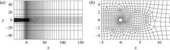
We consider optimal control of the unsteadiness of flow past a circular cylinder by imposing control on the surface of the cylinder. The domain and computational grid are shown in figure 1.
Spectral elements in the computational domain: (a) overall domain and (b) detail close to cylinder.

Spectral elements employing piecewise continuous nodal-based polynomial expansions within mapped-quadrilateral elemental subdomains are adopted for two-dimensional spatial discretization. Time integration is carried out using a velocity-correction scheme. Details of the discretization and its convergence properties (exponential in space, second order in time) are given in Blackburn & Sherwin (Reference Blackburn and Sherwin2004). The same numerics are used to compute base flows and the actions of the decomposed NS, linearized NS and adjoint operators. Since the unsteadiness in the region far downstream of the cylinder has limited influence on the dynamics around the cylinder, we adopt a weight function
 $$\begin{eqnarray}W(\boldsymbol{x})=\left\{\begin{array}{@{}ll@{}}1,\quad \quad & \text{for}~x<10,\\ \exp (-(x-10)^{2}),\quad \quad & \text{for}~x\geqslant 10.\end{array}\right.\end{eqnarray}$$
Therefore, for
 $x>10$
, the weight function rapidly reduces to zero and so the unsteadiness in this region is filtered. Further downstream extension of this ‘region of interest’ has negligible effect on the optimal control, as established in a separate set of tests. As should be apparent from (2.7), a longer time horizon
 ${\it\tau}$
is required to obtain an effective control when a longer downstream region is taken into account in the weight function.
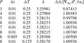
As a convergence test of the discretization and numerical method, we consider the unsteadiness
 $A$
(see (2.7)) as a function of the spectral polynomial order
 $P$
used in each spectral element, as reported in table 1, where we see that
 $A$
converges to four significant figures at
 $P=6$
.
Convergence of the unsteadiness
 $A$
and the gradient
 $\boldsymbol{{\rm\nabla}}_{\boldsymbol{u}_{\boldsymbol{n}}}\mathscr{L}$
with respect to spectral polynomial order
 $P$
, time step
 ${\rm\Delta}t$
and time interval to save the base flow
 ${\rm\Delta}T$
at
 $\mathit{Re}=100$
,
 ${\it\omega}=0$
and
 ${\it\tau}=80$
. The control cost is
 $E=0.001$
and
 $E=0.1$
for the convergence tests of the unsteadiness and the gradient respectively.

Also reported in table 1 is the convergence of
 ${\rm\Delta}A/[\boldsymbol{{\rm\nabla}}_{\boldsymbol{u}_{\boldsymbol{n}}}\mathscr{L},{\it\delta}u_{n}]$
. Here,
 ${\rm\Delta}A$
is calculated as
 ${\rm\Delta}A=A(\mathscr{N}(u_{n}+{\it\delta}u_{n}))-A(\mathscr{N}(u_{n}))$
, where
 ${\it\delta}u_{n}$
is a variation of the control with a small magnitude, and
 $\mathscr{N}(u_{n}+{\it\delta}u_{n})$
and
 $\mathscr{N}(u_{n})$
are obtained by integrating the decomposed NS equation;
 $\boldsymbol{{\rm\nabla}}_{\boldsymbol{u}_{\boldsymbol{n}}}\mathscr{L}$
is calculated following the procedure presented in § 2.2, where both the decomposed NS and adjoint equations are involved. Therefore, the convergence of
 ${\rm\Delta}A/[\boldsymbol{{\rm\nabla}}_{\boldsymbol{u}_{\boldsymbol{n}}}\mathscr{L},{\it\delta}u_{n}]$
to unity represents the correctness of the gradient
 $\boldsymbol{{\rm\nabla}}_{\boldsymbol{u}_{\boldsymbol{n}}}\mathscr{L}$
as well as the correct specification and accurate integration of the adjoint equation. We see that this gradient converges very well at
 $P>3$
. The energy cost is
 $E=0.1$
in this convergence test of the gradient, while in the test of convergence of
 $A$
, a smaller value of
 $E$
, that is
 $E=0.001$
, is used to reduce the number of optimization iterations. Considering both the convergence results and the computational costs, in all the following calculations, we adopt
 $P=6$
.
The time step
 ${\rm\Delta}t=0.01$
and the time interval used to save and reconstruct the base flow
 ${\rm\Delta}T=0.25$
(Mao, Sherwin & Blackburn Reference Mao, Sherwin and Blackburn2011) are also tested to be sufficiently small. In calculations at higher Reynolds number, e.g.
 $\mathit{Re}=1000$
, the time step is reduced to
 ${\rm\Delta}t=0.0016$
to avoid numerical divergence. Here, the Reynolds number is defined using the free-stream velocity and the diameter of the cylinder.
4. Results
In this section, we present the linear (sensitivity) and nonlinear optimal controls, and further discuss the physical mechanisms of the control. As mentioned previously, in this study we focus on control forcing that is spanwise-invariant (and therefore two-dimensional). Although we will consider three-dimensional flow, this assumption does preclude spanwise varying control action, which in other studies (Darekar & Sherwin Reference Darekar and Sherwin2001; Kim & Choi Reference Kim and Choi2005) has been observed to be an efficient form of boundary forcing.
4.1. Sensitivity
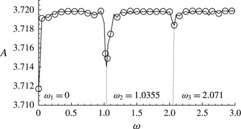
First, we consider the dependence of the control effect on the temporal frequency
 ${\it\omega}$
at a relatively small Reynolds number
 $\mathit{Re}=100$
, as illustrated in figure 2. A small control cost of
 $E=10^{-7}$
is adopted since the sensitivity is an optimal control only when the magnitude of the perturbation is small. As shall be later demonstrated in figure 4, the sensitivity almost overlaps with the nonlinear optimal control at such a low level of control cost, and therefore the frequency dependence of the sensitivity, at this level of control cost, is also relevant to the nonlinear optimal control. We observe that the unsteadiness reaches local minima at
 ${\it\omega}_{1}=0$
,
 ${\it\omega}_{2}=1.0355$
and
 ${\it\omega}_{3}=2.071$
. The first frequency corresponds to a steady control, the second corresponds to the vortex shedding frequency of the base flow, i.e.
 ${\it\omega}=2{\rm\pi}\mathit{St}=1.0355$
, where
 $\mathit{St}=0.1648$
is the Strouhal number for flow past a cylinder at
 $\mathit{Re}=100$
, and the third frequency is a higher harmonic of the shedding frequency.
Unsteadiness
 $A$
under control of the sensitivity at various values of
 ${\it\omega}$
at
 $\mathit{Re}=100$
,
 ${\it\tau}=80$
and
 $E=10^{-7}$
.

Since
 ${\it\omega}=0$
is the most effective frequency of the control perturbation and a full suppression of the unsteadiness can be achieved only with time-independent control forcing at this frequency (for non-zero frequencies, at least the velocity oscillation around the cylinder surface cannot be suppressed), in the following studies we adopt
 ${\it\omega}=0$
if not otherwise stated.
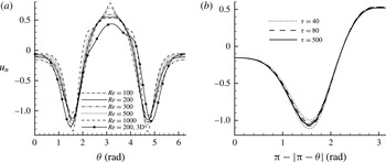
The distribution of the sensitivities at various Reynolds numbers is shown in figure 3(a). In this figure
 ${\it\theta}\in [0,2{\rm\pi}]$
is the azimuthal coordinate of the surface of the cylinder measured from the front stagnation point in the clockwise direction. Therefore,
 $0\leqslant {\it\theta}\leqslant {\rm\pi}$
and
 ${\rm\pi}\leqslant {\it\theta}\leqslant 2{\rm\pi}$
correspond to the upper surface from the front stagnation point to the trailing edge and the lower surface from the trailing edge to the front stagnation point respectively. This convention of
 ${\it\theta}$
is used in all the following figures. Further, in this and all the following figures on the distribution of the control, the solution is presented normalized such that
 $[u_{n},u_{n}]=1$
.
Distribution of the sensitivity of the normalized normal control on the surface of the cylinder at (a)
 ${\it\tau}=80$
and various Reynolds numbers and (b)
 $\mathit{Re}=100$
and various final times
 ${\it\tau}$
. Here,
 ${\it\theta}=0$
is the front stagnation point and
 ${\it\theta}={\rm\pi}$
is the trailing edge.

We see in figure 3(a) that for the parameters considered, the optimal perturbations are mostly concentrated upstream of the mean upper and lower separation points, i.e.
 ${\it\theta}\approx \pm 2$
, and the trailing edge
 ${\it\theta}={\rm\pi}$
, while a small proportion of the control is present at the front stagnation point
 ${\it\theta}=0$
. As the Reynolds number increases, the control around separation points and the trailing edge tends to increase while the component around the front stagnation point reduces. These distributions of the sensitivity indicate that the unsteadiness is most sensitive to boundary disturbance slightly upstream of the separation points, as has been observed in experiments on flow around a general axisymmetric bluff body at higher Reynolds number (Wilson et al.
Reference Wilson, Schatzmann, Arad, Seifert and Shtendel2013), and the trailing edge, while insensitive to boundary perturbations around the front stagnation point when
 $-{\rm\pi}/4<{\it\theta}<{\rm\pi}/4$
.
The slight asymmetry with respect to
 ${\it\theta}={\rm\pi}$
of the two-dimensional sensitivity in figure 3(a) arises as a result of the non-integer number of periods of shedding contained in the time interval
 $[0,{\it\tau}]$
, which therefore leads to differences in the upper- and lower-surface control velocities. We also note that the temporal function (2.3) is not exactly periodic since there is an exponential envelope at startup. In figure 3(b) we plot the two halves of the sensitivity on the same axis so that we can see the asymmetry. We observe that at
 ${\it\tau}=40$
the dotted lines do not overlap, but it is clear that at higher values of
 ${\it\tau}$
, when more periods are included, the sensitivities on the upper and lower surfaces of the cylinder overlap each other and the sensitivity becomes symmetric.
For
 $\mathit{Re}>190$
, the uncontrolled base flow is unstable to three-dimensional disturbances (Barkley & Henderson Reference Barkley and Henderson1996) and therefore a three-dimensional base flow becomes a more appropriate control objective at high Reynolds numbers. The sensitivity of a three-dimensional base flow at
 $\mathit{Re}=200$
is also presented in figure 3(a). This base flow is obtained by adopting a three-dimensional domain, whose spanwise extent is
 $2{\rm\pi}/1.58$
so as to accommodate unstable three-dimensional modes (Barkley & Henderson Reference Barkley and Henderson1996), imposing periodicity and using 32 complex Fourier modes in the spanwise direction. The uncontrolled three-dimensional base flow will be discussed further in relation to figure 9(a). From the formulation shown in § 2, only the Fourier mode with zero spanwise wavenumber is required in the calculation since the control activation is spanwise-invariant. We see in figure 3(a) that the three-dimensionality does not yield a significant change in the distribution of the sensitivity.
4.2. Distribution of the optimal control
Figure 4 presents a comparison of the sensitivity and nonlinear optimal control at various values of
 $E$
. Due to the computational cost of the nonlinear optimal control, the final time is reduced to
 ${\it\tau}=30$
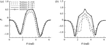
for all the nonlinear calculations. We notice that the nonlinear optimal control at small control magnitude overlaps with the sensitivity, and deviates from the sensitivity as
 $E$
increases. In figure 4(a), it is observed that at a relatively low Reynolds number
 $\mathit{Re}=100$
, the sensitivity can be a reasonably good approximation of the nonlinear optimal control over the range of control cost considered. However, the deviation of the nonlinear optimal control from the sensitivity becomes much more dramatic at
 $\mathit{Re}=1000$
, indicating that the linear regime where the sensitivity acts as an optimal solution reduces at larger Reynolds number. As the control cost
 $E$
is increased, the control magnitude around the front stagnation point reduces, and the peaks of the control around the separation points move slightly towards the rear of the cylinder. At
 $E=0.02$
, the nonlinear optimal control expands to the region downstream of the separation points in the form of suction, and changes to blowing when approaching the trailing edge (see figure 4
b), instead of sharply concentrating around the separation point, i.e. the linearly most sensitive region.
Deviation of the nonlinear solutions from the sensitivity at
 ${\it\tau}=30$
and (a)
 $\mathit{Re}=100$
and (b)
 $\mathit{Re}=1000$
.

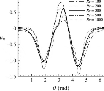
From figure 5, we see that the locations of the peak around the separation points are not very sensitive to the Reynolds number, even though at higher Reynolds numbers the blowing around the trailing edge
 ${\it\theta}={\rm\pi}$
becomes stronger. In addition, we observe that at higher Reynolds number or control magnitude, the control becomes more asymmetric. Once again, this can be attributed to the fact that the flow is periodic and the control effects of the upper and lower surfaces are asynchronous. Therefore, at
 $t=0$
, one side of the cylinder has a greater ability to control the flow. We note that since this asymmetry changes from case to case, it is unlikely to be attributable to the asymmetry of the grid.
Distribution of the nonlinear optimal controls at
 ${\it\tau}=30$
,
 $E=0.05$
and various Reynolds numbers.

4.3. Control effects of the optimal control
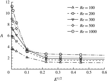
The control effect of the nonlinear optimal control on the unsteadiness
 $A$
(see (2.7)), which we recall denotes the difference between the average of the square integral of the velocity and the square integral of the average velocity over a time interval
 ${\it\tau}$
, is presented in figure 6. We observe that the magnitude of
 $A$
increases with Reynolds number, indicating that the flow becomes more unsteady at higher Reynolds numbers. Under the action of the nonlinear control,
 $A$
drops significantly, and the control effects are more evident at higher Reynolds numbers. Over small values of control cost, the nonlinear optimal control can be approximated by the sensitivity, and the change of
 $A$
is a linear function of the magnitude of the control, measured by
 $E^{1/2}$
. It is seen that this linear relation is preserved until
 $E=0.01$
, above which the unsteadiness drops much more slowly. For
 $E>0.1$
,
 $A$
becomes almost constant, indicating that the vortex shedding has been completely suppressed while the unsteadiness at the beginning of imposing control is uncontrollable.
Optimally controlled unsteadiness
 $A(\boldsymbol{u})$
as a function of
 $E^{1/2}$
, which measures the magnitude of the control.

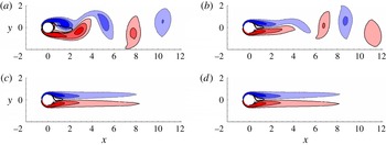
Four vorticity plots at times
 $t=0,10,30$
and 50 under the action of the nonlinear optimal control at
 $\mathit{Re}=100$
,
 ${\it\tau}=30$
and
 $E=0.05$
are shown in figure 7. We observe that the vortex shedding is gradually weakened before being completely suppressed to form a pair of elongated shear layers at
 $t=30$
. After this time the flow maintains a steady state. We note that under the action of the control, the recirculation bubble downstream of the cylinder extends to
 $x<2$
. This bubble is much smaller than the bubble in the uncontrolled steady flow, which reaches
 $x=6.6$
, obtained by numerically suppressing unsteadiness (Fornberg Reference Fornberg1991; Gajjar & Azzam Reference Gajjar and Azzam2004). The reduction of the length of the bubble significantly attenuates the inflection point instabilities associated with the recirculation zone, and therefore this stabilized flow is expected to be more stable than the uncontrolled steady flow, as will be verified later. In the controlled flow, the vertical motion associated with vortex shedding, which extracts energy from the streamwise flow, is suppressed, and therefore a drag reduction can be expected, as will be discussed later in § 4.5.
Contours of spanwise vorticity for the controlled flow at
 $\mathit{Re}=100$
,
 ${\it\tau}=30$
and
 $E=0.05$
. Panels (a), (b), (c) and (d) correspond to times
 $t=0$
, 10, 30 and 50 respectively. Dashed lines, light solid lines and thick solid lines represent negative spanwise vorticity, positive spanwise vorticity and zero streamwise velocity respectively. The contour levels for spanwise vorticity are
 $[-2,-1.2,-0.4,0.4,1.2,2]$
.

Sensitivity of the control effect with respect to the starting time or the phase of a vortex shedding period was also tested. In this test the initial conditions adopted in figure 7 were shifted by a quarter or half of a shedding period. We observed that the process of suppression of shedding was only slightly different, but the final control effect was independent of the starting time, indicating that the control is robust with respect to the starting time of imposing control.
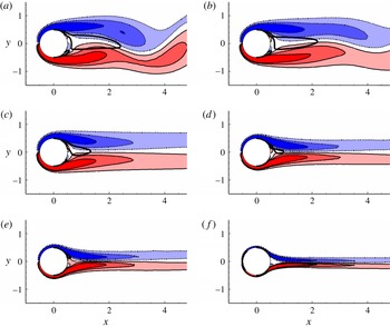
The optimal controlled flow at various control costs and Reynolds numbers is illustrated in figure 8. We see that at
 $\mathit{Re}=100$
, as
 $E$
increases, the shedding is gradually weakened, and at
 $E=0.05$
, for the Reynolds numbers considered, the vortex shedding can be completely suppressed (at
 $\mathit{Re}=1000$
, complete suppression of shedding can be achieved at
 $E=0.02$
). We further observe that the recirculation bubble downstream of the cylinder shrinks at higher Reynolds numbers, and at
 $\mathit{Re}=300$
, this recirculation zone disappears, and so does the instability associated with recirculation bubbles. It is also noticeable that the shear layers shed from the surface of the cylinder become thinner and more elongated at higher Reynolds numbers.
Contours of spanwise vorticity under the nonlinear optimal control at (a)
 $(\mathit{Re},E)=(100,0.01)$
, (b)
 $(\mathit{Re},E)=(100,0.02)$
, (c)
 $(\mathit{Re},E)=(100,0.05)$
, (d)
 $(\mathit{Re},E)=(200,0.05)$
, (e)
 $(\mathit{Re},E)=(300,0.05)$
and (f)
 $(\mathit{Re},E)=(1000,0.05)$
. The result is collected at
 $t={\it\tau}=30$
. Dashed lines, light solid lines and thick solid lines represent negative spanwise vorticity, positive spanwise vorticity and zero streamwise velocity respectively. The contour levels for spanwise vorticity are
 $[-2,-1.2,-0.4,0.4,1.2,2]$
.

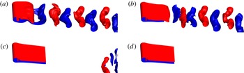
After testing the control effects of the nonlinear optimal control on unsteadiness of two-dimensional flows, we also determined whether these optimal two-dimensional controls are effective in fully developed three-dimensional flows. Figure 9 shows the controlled and uncontrolled three-dimensional flow at
 $\mathit{Re}=200$
and
 $E=0.05$
. The spanwise length of the domain is set to
 $2{\rm\pi}/1.58$
, and 32 complex Fourier modes are applied to discretize the spanwise direction, the same as in the calculation of the sensitivity of three-dimensional flow (see § 4.1). The three-dimensionality of the uncontrolled flow can be clearly identified in figure 9(a), corresponding to the initial solution when the nonlinear control was activated. Under the action of the nonlinear optimal control, we see that the unsteady structures are washed downstream and the flow pattern is stabilized to a two-dimensional steady flow, as discussed above for the two-dimensional case.
Isosurfaces of spanwise vorticity −0.6 (blue) and 0.6 (red) of three-dimensional flow under nonlinear optimal control at
 $\mathit{Re}=200$
,
 ${\it\tau}=30$
and time (a)
 $t=0$
, (b)
 $t=10$
, (c)
 $t=20$
and (d)
 $t=30$
.

In related flow stabilization works, sensitivity tests of global stability of a steady base flow with respect to external forcing (Marquet et al.
Reference Marquet, Sipp and Jacquin2008) or steady boundary forcing (Marquet & Sipp Reference Marquet, Sipp, Schlatter and Henningson2010) have been conducted, and the calculated sensitivity was demonstrated to be effective in stabilizing the flow and subsequently eliminating vortex shedding at
 $47\leqslant \mathit{Re}\leqslant 80$
. In the current method, the controlled flow reaches steady states and therefore enables a global stability study.
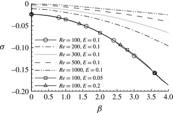
Asymptotic stability tests of the stabilized steady flow to two-dimensional and three-dimensional perturbations were undertaken, as presented in figure 10, where
 ${\it\sigma}$
denotes the maximum growth rate of the most unstable eigenmode and
 ${\it\beta}$
represents the spanwise wavenumber of different eigenmodes. We see that the stabilized flow is asymptotically stable over the cases considered. The largest energy growth rate corresponding to the most unstable mode changes slightly with respect to the control cost used to obtain the steady flow, and the maximum value of these growth rates is obtained at
 ${\it\beta}=0$
, corresponding to a two-dimensional perturbation. As the Reynolds number increases, however, the most unstable eigenmodes become more unstable, but over the parameters considered, the controlled flow is always asymptotically stable.
Asymptotic stability of the steady flow subjected to the nonlinear optimal control. Here,
 ${\it\sigma}$
denotes the maximum growth rate of the most unstable eigenmode at spanwise wavenumber
 ${\it\beta}$
.

4.4. Mechanism of the optimal control
As already presented, the distribution of the optimal control changes notably with increase of the control cost. At low control magnitudes, e.g.
 $E=10^{-5}$
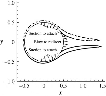
, the nonlinear optimal control, which can be well approximated by the sensitivity, consists primarily of low-magnitude leading edge suction, higher-magnitude (slightly upstream) separation point suction and trailing edge blowing, as shown in figure 4. The leading edge suction reduces the strength of the shear layer, the separation point suction delays the separation and the trailing edge blowing pushes the upper and lower shear layers away from each other. Clearly, all these mechanisms act on the uncontrolled flow, and the response of the flow to the control, which can be significant at larger control costs, is not counted, due to the linear nature of this control.
Schematic of the boundary layer attachment–redirection mechanism of the nonlinear control. Thick dashed lines and thick solid lines are contour lines for vorticity −3 and 3 at
 $\mathit{Re}=1000$
under nonlinear control with
 $E=0.05$
and
 $t={\it\tau}=30$
. Dotted lines denote the nonlinear optimal control, while lines inside and outside the cylinder represent suction and blowing respectively, as indicated by the arrows.

As discussed above, for higher values of control cost, the control spreads to the downstream region of the uncontrolled separation points and keeps the shear layer attached to the cylinder surface, while the blowing around the trailing edge redirects the two shear layers to a pair of parallel shear layers in the wake. The spreading of the control downstream of the uncontrolled separation point is a clear nonlinear mechanism, i.e. as separation is delayed by control slightly upstream of the uncontrolled separation point, the downstream control acts on the controlled flow and further delays separation. We notice that this continuous delay of separation is essential to the successful suppression of vortex shedding and cannot be predicted in the linear control (sensitivity).
From the stabilized flow around the cylinder illustrated in figure 8, we see that as the Reynolds number increases, the attachment point of the stabilized flow moves downstream towards the trailing edge, resulting in shear layers being deflected by a larger angle to form a parallel pair of shear layers. Therefore, a stronger redirection force is required, which is consistent with the observation in figure 5 that the magnitude of the nonlinear optimal control around the trailing edge (the blowing) increases with the Reynolds number. It is worth noting that the control, which induces separation delay and boundary layer redirection, acts mainly on the separating shear layers. This attachment–redirection control mechanism, as schematically plotted in figure 11, is observed for all the Reynolds numbers considered, and might be expected at higher Reynolds numbers.
4.5. Controlled drag
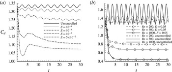
When the vortex shedding is weakened, it can be expected that the forces acting on the cylinder become less oscillatory, as illustrated in figure 12. We see that as the control cost increases, the oscillation magnitude of drag (and lift which is not presented here) reduces. At
 $E=0.05$
, where the vortex shedding is completely suppressed, the force coefficient approaches steady values.
Development of the drag coefficient
 $C_{d}$
at (a)
 $\mathit{Re}=100$
and various control costs, and (b)
 $E=0.05$
and various Reynolds numbers.

It is worth noting that under the control, the magnitude of drag reduces significantly, indicating a strong correlation between unsteadiness and drag. This correlation can be explained in the view of energy, i.e. the unsteady vortex shedding is associated with vertical flow, whose energy is extracted from the streamwise flow, and therefore decelerates the streamwise flow and generates drag. The variability of the forces under the nonlinear optimal control at different Reynolds numbers is illustrated in figure 12(b). We see that at control cost
 $E=0.05$
, the drag is reduced by approximately 20 % at
 $\mathit{Re}=100$
and over 70 % at
 $\mathit{Re}=1000$
(similar results are obtained at
 $E=0.02$
), indicating that a large proportion of the drag is associated with the unsteadiness in the wake. If one decomposes the drag into form and viscous components, it is found that the control reduces the form drag significantly but increases the viscous drag, both effects due to the suppression of separation.
5. Discussion and conclusions
We have investigated algorithms to optimally suppress unsteadiness modelled as fluctuation energy in incompressible flow. The control is introduced in the form of wall-normal boundary velocity perturbations with a prescribed magnitude and temporal frequency. We consider both the linear optimal control, i.e. the sensitivity, and the nonlinear optimal control.
The sensitivity represents the gradient of the unsteadiness with respect to the control and only requires an integration of a simplified adjoint equation without any iterative optimization procedure. In the derivation of the simplified adjoint equation for the sensitivity, the control-induced flow is assumed to be small compared with the uncontrolled flow, and therefore this sensitivity is a linearly optimal control, which is a good approximation of the nonlinear optimal control when the control magnitude is small enough.
The nonlinear optimal control uses the decomposed NS equation and linearized NS equation and the adjoint as the governing equations. The adjoint equation, as well as its outflow boundary condition, is related with the uncontrolled and control-induced velocity, and therefore the development history of the control-induced flow must be recorded to solve the decomposed NS equation. In this scheme, a step length optimal in a linear sense can be calculated by integrating the linearized NS equation twice. Therefore, in each optimization step, the decomposed NS equation is at least called once, the adjoint solver is called once and the linearized NS equation solver is called twice, resulting in four calls of the governing equations in each optimization step.
The algorithms were applied to control the unsteady flow past a circular cylinder for
 $\mathit{Re}\leqslant 1000$
. From the distribution of the sensitivity around the cylinder surface, it was observed that the control is mostly located around the separation points and the trailing edge, while a small proportion of the control is around the front stagnation point. On testing the control effectiveness of the sensitivity at small values of control cost, it was observed that the most effective control occurs at frequencies of
 ${\it\omega}=0$
,
 ${\it\omega}=1.0355$
and
 ${\it\omega}=2.071$
. The first frequency corresponds to a steady control, the second is the frequency of vortex shedding in the uncontrolled base flow and the last one is a higher harmonic of the vortex shedding frequency. Since steady control is the globally most effective one, in all the other calculations we set the frequency of the control to
 ${\it\omega}=0$
. The sensitivity was not completely symmetric on the upper and lower surfaces of the cylinder due to the imposition of a finite value of the control time interval,
 ${\it\tau}$
, which was not commensurate with the periodic shedding from the cylinder. As we increased
 ${\it\tau}$
, the upper and lower parts of the sensitivity became more symmetric. The sensitivity was also found to be insensitive to the Reynolds number in the range
 $\mathit{Re}=100{-}1000$
, and the three-dimensional development of the uncontrolled base flow did not yield significant changes to the sensitivity as tested at a Reynolds number of 200.
Unlike the sensitivity, whose shape is independent of the control cost, the nonlinear optimal control is a function of the control cost. The nonlinear optimal control is concentrated downstream of the separation points and it contains a suction component to postpone separation and a trailing edge blowing component to redirect the separated shear layers to a pair of parallel shear layers. On comparing the sensitivity and nonlinear optimal control at various control costs, it is confirmed that at small values of the control cost, the two solutions overlap; at higher levels of control cost, the nonlinear optimal control deviates from the sensitivity, in a more dramatic manner at higher Reynolds number.
Under the nonlinear optimal control, the vortex shedding over the range of the Reynolds number considered can be completely suppressed at
 $E=0.05$
. At the highest Reynolds number tested, i.e.
 $\mathit{Re}=1000$
, complete suppression of vortex shedding can be achieved at
 $E=0.02$
, corresponding to an r.m.s. value of the control of 0.08, normalized by the free-stream velocity, with control effectiveness, defined as the ratio of control-reduced drag power and input power (see appendix C), of
 $E_{C}=3.65$
. The fully developed three-dimensional flow was also tested and similar control effects could be observed.
The asymptotic stability characteristics of the stabilized flow were studied and we observed that the controlled steady flow is stable to both two- and three-dimensional perturbations by calculating the largest growth rate of global modes of the steady flow. The most unstable mode is a two-dimensional mode and its growth rate changes slightly with the control cost used to obtain the steady flow. As the Reynolds number increases, the growth rates of eigenmodes of the stabilized flow approach the unstable threshold
 ${\it\sigma}=0$
, but over the parameters considered, the growth rates of all the eigenmodes are negative.
The force acting on the cylinder under control was also investigated. It was noticed that as the vortex shedding was suppressed, both the oscillation and the mean value of drag were reduced. At
 $\mathit{Re}=1000$
and
 $E=0.02$
, the drag reduction was over 70 %.
Acknowledgements
We would like to acknowledge financial support from the Australian Research Council through Discovery Program Grant DP1094851, and from Australia’s National Computational Infrastructure via Merit Allocation Scheme Grant D77. S.J.S. would like to acknowledge financial support under EPSRC grant EP/H050507/1.
Appendix A. Derivation of (2.13)
The variation of the second term on the right-hand side of (2.11) with respect to the perturbation velocity induced by the control is
 $$\begin{eqnarray}{\it\delta}\langle \boldsymbol{u}^{\ast },N(\boldsymbol{u})\rangle ({\it\delta}\boldsymbol{u})=\langle {\it\delta}\boldsymbol{u},\boldsymbol{{\rm\nabla}}\boldsymbol{u}\boldsymbol{\cdot }\boldsymbol{u}^{\ast }\rangle +\langle \boldsymbol{u},\boldsymbol{{\rm\nabla}}{\it\delta}\boldsymbol{u}\boldsymbol{\cdot }\boldsymbol{u}^{\ast }\rangle .\end{eqnarray}$$
Substituting the formulation
 $$\begin{eqnarray}\boldsymbol{{\rm\nabla}}{\it\delta}\boldsymbol{u}\boldsymbol{\cdot }\boldsymbol{u}^{\ast }=\boldsymbol{{\rm\nabla}}({\it\delta}\boldsymbol{u}\boldsymbol{\cdot }\boldsymbol{u}^{\ast })-\boldsymbol{{\rm\nabla}}\boldsymbol{u}^{\ast }\boldsymbol{\cdot }{\it\delta}\boldsymbol{u}\end{eqnarray}$$
into (A 1), we have
 $$\begin{eqnarray}{\it\delta}\langle \boldsymbol{u}^{\ast },N(\boldsymbol{u})\rangle ({\it\delta}\boldsymbol{u})=\langle {\it\delta}\boldsymbol{u},\boldsymbol{{\rm\nabla}}\boldsymbol{u}\boldsymbol{\cdot }\boldsymbol{u}^{\ast }-\boldsymbol{u}\boldsymbol{\cdot }\boldsymbol{{\rm\nabla}}\boldsymbol{u}^{\ast }\rangle +\langle \boldsymbol{u},\boldsymbol{{\rm\nabla}}({\it\delta}\boldsymbol{u}\boldsymbol{\cdot }\boldsymbol{u}^{\ast })\rangle .\end{eqnarray}$$
Then, substituting
 $$\begin{eqnarray}\boldsymbol{u}\boldsymbol{\cdot }\boldsymbol{{\rm\nabla}}({\it\delta}\boldsymbol{u}\boldsymbol{\cdot }\boldsymbol{u}^{\ast })=\boldsymbol{{\rm\nabla}}\boldsymbol{\cdot }(\boldsymbol{u}{\it\delta}\boldsymbol{u}\boldsymbol{\cdot }\boldsymbol{u}^{\ast })-(\boldsymbol{{\rm\nabla}}\boldsymbol{\cdot }\boldsymbol{u}){\it\delta}\boldsymbol{u}\boldsymbol{\cdot }\boldsymbol{u}^{\ast }\end{eqnarray}$$
into (A 3) and considering the divergence-free condition of
 $\boldsymbol{u}$
, we obtain
 $$\begin{eqnarray}{\it\delta}\langle \boldsymbol{u}^{\ast },N(\boldsymbol{u})\rangle ({\it\delta}\boldsymbol{u})=\langle {\it\delta}\boldsymbol{u},\boldsymbol{{\rm\nabla}}\boldsymbol{u}\boldsymbol{\cdot }\boldsymbol{u}^{\ast }-\boldsymbol{u}\boldsymbol{\cdot }\boldsymbol{{\rm\nabla}}\boldsymbol{u}^{\ast }\rangle +{\it\tau}^{-1}\int _{0}^{{\it\tau}}\int _{{\it\Omega}}\boldsymbol{{\rm\nabla}}\boldsymbol{\cdot }(\boldsymbol{u}{\it\delta}\boldsymbol{u}\boldsymbol{\cdot }\boldsymbol{u}^{\ast })\,\text{d}V\,\text{d}t.\end{eqnarray}$$
Then, implementing the divergence theorem, we reach (2.13):
 $$\begin{eqnarray}{\it\delta}\langle \boldsymbol{u}^{\ast },N(\boldsymbol{u})\rangle ({\it\delta}\boldsymbol{u})=\langle {\it\delta}\boldsymbol{u},\boldsymbol{{\rm\nabla}}\boldsymbol{u}\boldsymbol{\cdot }\boldsymbol{u}^{\ast }-\boldsymbol{u}\boldsymbol{\cdot }\boldsymbol{{\rm\nabla}}\boldsymbol{u}^{\ast }\rangle +{\it\tau}^{-1}\int _{0}^{{\it\tau}}\int _{\partial {\it\Omega}}(\boldsymbol{n}\boldsymbol{\cdot }\boldsymbol{u})({\it\delta}\boldsymbol{u}\boldsymbol{\cdot }\boldsymbol{u}^{\ast })\,\text{d}S\,\text{d}t.\end{eqnarray}$$
Appendix B. Procedure to calculate the nonlinear optimal control
The numerical procedure to calculate the nonlinear optimal control is as follows.
-
(1) Calculate the averaged base flow velocity
 $\boldsymbol{U}_{a}$
over time
$0\leqslant t\leqslant {\it\tau}$
.
-
(2) Initialize
$u_{n}$
by random noise. -
(3) Integrate (2.5) to calculate and save
$\boldsymbol{u}(t)=\mathscr{N}(u_{n})$
for the time interval
$[0,{\it\tau}]$
. -
(4) Calculate the total unsteadiness through (2.7).
-
(5) Solve the adjoint equation (2.15) to calculate the adjoint variables
$\boldsymbol{u}^{\ast }$
and
$p^{\ast }$
. It should be noted that
$\boldsymbol{u}(t)$
is used in this step. -
(6) Substitute
$\boldsymbol{u}^{\ast }$
and
$p^{\ast }$
into (2.17) to calculate
$g$
. -
(7) Considering
$gf(t,{\it\omega})\boldsymbol{n}$
and
$u_{n}f(t,{\it\omega})\boldsymbol{n}$
as boundary conditions for the control boundary and
$\boldsymbol{U}+\boldsymbol{u}^{k}$
as the base flow, integrate (2.22) to obtain
$\mathscr{M}_{\boldsymbol{U}+\boldsymbol{u}}(g)$
and
$\mathscr{M}_{\boldsymbol{U}+\boldsymbol{u}}(u_{n}^{k})$
. -
(8) Substitute
$\mathscr{M}_{\boldsymbol{U}+\boldsymbol{u}}(g)$
and
$\mathscr{M}_{\boldsymbol{U}+\boldsymbol{u}}(u_{n}^{k})$
into (2.21) to obtain
$\boldsymbol{u}_{l}^{k+1}$
and then substitute
$\boldsymbol{u}_{l}^{k+1}$
into (2.7) to calculate the optimal (in linear sense) value of the step length
${\it\alpha}$
. -
(9) Update the control following (2.19) and the perturbation velocity
$\boldsymbol{u}^{k+1}$
following (2.20), where the governing equation (2.5) is called. -
(10) Substitute
$\boldsymbol{u}^{k+1}$
into (2.7) to check whether the unsteadiness is reduced. If not, reduce the value of
${\it\alpha}$
and repeat steps 9 and 10 until the unsteadiness reduces. -
(11) Repeat steps 5–10 until the solution
$u_{n}$
converges.


Appendix C. Cost/benefit analysis of control
To calculate the time-average cost and benefit of the control, we consider the mean flow momentum and energy equations for flow inside a time-invariant domain in an inertial reference frame. If the flow is decomposed into a time mean and a fluctuation as
 $\boldsymbol{u}=\overline{\boldsymbol{u}}+\boldsymbol{u}^{\prime }$
,
 $p=\overline{p}+p^{\prime }$
, with kinetic energy per unit mass of the mean flow
 $\overline{q}=(\overline{\boldsymbol{u}}\boldsymbol{\cdot }\overline{\boldsymbol{u}})/2$
, and time-mean strain rate
 $\overline{\boldsymbol{S}}=[\boldsymbol{{\rm\nabla}}\overline{\boldsymbol{u}}+(\boldsymbol{{\rm\nabla}}\overline{\boldsymbol{u}})^{\text{T}}]/2$
, then the per-unit-mass equations for time-average momentum and kinetic energy of incompressible flow are respectively
 $$\begin{eqnarray}\boldsymbol{{\rm\nabla}}\boldsymbol{\cdot }\overline{\boldsymbol{u}}\,\overline{\boldsymbol{u}}+{\it\rho}^{-1}\boldsymbol{{\rm\nabla}}\overline{p}-2{\it\nu}\boldsymbol{{\rm\nabla}}\boldsymbol{\cdot }\overline{\boldsymbol{S}}+\boldsymbol{{\rm\nabla}}\boldsymbol{\cdot }\overline{\boldsymbol{u}^{\prime }\boldsymbol{u}^{\prime }}=\mathbf{0}\end{eqnarray}$$
and
 $$\begin{eqnarray}\overline{\boldsymbol{u}}\boldsymbol{\cdot }\boldsymbol{{\rm\nabla}}\overline{q}+\boldsymbol{{\rm\nabla}}\boldsymbol{\cdot }[{\it\rho}^{-1}\overline{p}\,\overline{\boldsymbol{u}}-2{\it\nu}\overline{\boldsymbol{S}}\boldsymbol{\cdot }\overline{\boldsymbol{u}}+\overline{\boldsymbol{u}^{\prime }\boldsymbol{u}^{\prime }}\boldsymbol{\cdot }\overline{\boldsymbol{u}}]+2{\it\nu}\overline{\boldsymbol{S}}:\overline{\boldsymbol{S}}-\overline{\boldsymbol{u}^{\prime }\boldsymbol{u}^{\prime }}:\overline{\boldsymbol{S}}=0,\end{eqnarray}$$
or, adopting the notations
 $\overline{{\bf\tau}}=2{\it\nu}\overline{\boldsymbol{S}}-\overline{\boldsymbol{u}^{\prime }\boldsymbol{u}^{\prime }}$
and
 $\overline{{\bf\tau}}_{n}=\overline{{\bf\tau}}\boldsymbol{\cdot }\boldsymbol{n}$
, where
 $\boldsymbol{n}$
is the domain’s unit outward normal vector,
 $$\begin{eqnarray}\boldsymbol{{\rm\nabla}}\boldsymbol{\cdot }\overline{\boldsymbol{u}}\,\overline{\boldsymbol{u}}+{\it\rho}^{-1}\boldsymbol{{\rm\nabla}}\overline{p}-\overline{{\bf\tau}}=\mathbf{0}\end{eqnarray}$$
and
 $$\begin{eqnarray}\overline{\boldsymbol{u}}\boldsymbol{\cdot }\boldsymbol{{\rm\nabla}}\overline{q}+\boldsymbol{{\rm\nabla}}\boldsymbol{\cdot }[{\it\rho}^{-1}\overline{p}\,\overline{\boldsymbol{u}}-\overline{{\bf\tau}}\boldsymbol{\cdot }\overline{\boldsymbol{u}}]+\overline{{\bf\tau}}:\overline{\boldsymbol{S}}=0.\end{eqnarray}$$
Integrating over the control volume and using the divergence theorem, one obtains the integrated forms of the momentum and energy equations,
 $$\begin{eqnarray}\oint \overline{\boldsymbol{u}}\,\overline{\boldsymbol{u}}\boldsymbol{\cdot }\boldsymbol{n}\,\text{d}S+{\it\rho}^{-1}\oint \overline{p}\boldsymbol{n}\,\text{d}S-\oint \overline{{\bf\tau}}_{n}\,\text{d}S=\mathbf{0}\end{eqnarray}$$
and
 $$\begin{eqnarray}\oint \overline{q}\,\overline{\boldsymbol{u}}\boldsymbol{\cdot }\boldsymbol{n}\,\text{d}S+{\it\rho}^{-1}\oint \overline{p}\,\overline{\boldsymbol{u}}\boldsymbol{\cdot }\boldsymbol{n}\,\text{d}S-\oint \overline{{\bf\tau}}_{n}\boldsymbol{\cdot }\overline{\boldsymbol{u}}\,\text{d}S+\int _{V}\overline{{\bf\tau}}:\overline{\boldsymbol{S}}\,\text{d}V=0,\end{eqnarray}$$
where
 $S$
is the domain boundary and
 $V$
is its volume. The volume integral in (C 6) represents the sum of mean-flow viscous dissipation and drain of energy from the mean flow to the fluctuating flow.
In our analysis, the domain contains a single immersed body (circular cylinder) that may, in the controlled case, have a permeable surface over which fluid can flow. For further insight, we may decompose the domain boundary into
 $S_{O}$
, which is the domain’s outer or far-field boundary, and
 $S_{B}$
, which is the boundary surface around the enclosed body. The surface integrals above may then be decomposed into sums of integrals over these two subsets. For (C 5) we can then write
 $\boldsymbol{F}_{O}+\boldsymbol{F}_{B}=\mathbf{0}$
, where
 $$\begin{eqnarray}\displaystyle & \displaystyle \boldsymbol{F}_{0}=\oint \overline{\boldsymbol{u}}\,\overline{\boldsymbol{u}}\boldsymbol{\cdot }\boldsymbol{n}\,\text{d}S_{O}+{\it\rho}^{-1}\oint \overline{p}\boldsymbol{n}\,\text{d}S_{O}-\oint \overline{{\bf\tau}}_{n}\,\text{d}S_{O}, & \displaystyle\end{eqnarray}$$
 $$\begin{eqnarray}\displaystyle & \displaystyle \boldsymbol{F}_{B}=\oint \overline{\boldsymbol{u}}\,\overline{\boldsymbol{u}}\boldsymbol{\cdot }\boldsymbol{n}\,\text{d}S_{B}+{\it\rho}^{-1}\oint \overline{p}\boldsymbol{n}\,\text{d}S_{B}-\oint \overline{{\bf\tau}}_{n}\,\text{d}S_{B}, & \displaystyle\end{eqnarray}$$
 $\boldsymbol{F}_{B}$
represents the time-average force (per unit mass) exerted by the fluid on the contained body (instead – due to the sign convention adopted – of the force exerted by the body on the fluid). We note that since the body surface may be permeable,
 $\boldsymbol{F}_{B}$
can contain terms associated with both time-average and fluctuating velocities; these in turn would be associated with momentum transfers (and forces) internal to the body, and so their inclusion in the mean body-force term is sensible. Moreover, we note that, unlike the case for solid boundaries, there may be surface-normal viscous tractions acting on a permeable body, and that related work terms also appear in (C 6).
If we take the far-field fluid to be at rest and the domain (and body) to be translating with velocity
 $-\boldsymbol{U}_{\infty }$
, then the drag power per unit mass required to drive the body is
 $P_{D}=\boldsymbol{F}_{B}\boldsymbol{\cdot }\boldsymbol{U}_{\infty }$
. The difference between the drag powers in the uncontrolled and controlled cases,
 $P_{D_{U}}-P_{D_{C}}$
, is the physical benefit to be obtained through control.
Now we turn to assessing the physical cost, which is the blowing power required at the cylinder. We split the surface integrals in (C 6) into two parts. Writing
 $$\begin{eqnarray}\displaystyle & \displaystyle {\dot{W}}_{0}=\oint q\overline{\boldsymbol{u}}\boldsymbol{\cdot }\boldsymbol{n}\,\text{d}S_{O}+{\it\rho}^{-1}\oint \overline{p}\,\overline{\boldsymbol{u}}\boldsymbol{\cdot }\boldsymbol{n}\,\text{d}S_{O}-\oint \overline{{\bf\tau}}_{n}\boldsymbol{\cdot }\overline{\boldsymbol{u}}\,\text{d}S_{O}, & \displaystyle\end{eqnarray}$$
 $$\begin{eqnarray}\displaystyle & \displaystyle {\dot{W}}_{B}=\oint q\overline{\boldsymbol{u}}\boldsymbol{\cdot }\boldsymbol{n}\,\text{d}S_{B}+{\it\rho}^{-1}\oint \overline{p}\,\overline{\boldsymbol{u}}\boldsymbol{\cdot }\boldsymbol{n}\,\text{d}S_{B}-\oint \overline{{\bf\tau}}_{n}\boldsymbol{\cdot }\overline{\boldsymbol{u}}\,\text{d}S_{B}, & \displaystyle\end{eqnarray}$$
 $-{\dot{W}}_{B}$
.
Finally, we come to a definition of control effectiveness, which is the benefit of control divided by its cost:
 $$\begin{eqnarray}E_{C}=-(P_{D_{U}}-P_{D_{C}})/{\dot{W}}_{B}.\end{eqnarray}$$
(We note that it is possible to obtain a negative value for
 $E_{C}$
.) The control effectiveness of the nonlinear optimal control at
 $\mathit{Re}=1000$
and
 $E=0.02$
is found to be
 $E_{C}=3.65$
. It is worth noting that this effectiveness does not consider the actuator efficiency and therefore is an upper-limit value.
In practice, we typically compute all the integrals in (C 6) as volume integrals, relying on the divergence theorem and a separate computation of
 ${\dot{W}}_{O}$
to find
 ${\dot{W}}_{B}$
.