Hierarchical structure from prokaryotes to multicellular organisms

Until the 1960s the idea that complexity increases in evolution was widely accepted among evolutionary biologists. Numerous examples of increase in complexity were given by Lamarck, Darwin, Cope, Spencer, Gregory, Julian Huxley, Simpson and many others, and the consensus extended well beyond biologists. However, more recently, attempts to define complexity and to demonstrate its increase has led many authors to doubt that any increase actually took place. McShea (Reference McShea1991) contrasted the generality of the consensus with the paucity of the evidence and raised two main criticisms.

First, many examples were deliberately chosen in order to make a case for a uniform trend occurring in all lineages at all times, so neglecting many counter-examples. For instance, the skulls of Devonian fishes had more bones and were more complex than the human skull (Williams Reference Williams1966). Therefore, the case for a strictly uniform trend in complexity must be replaced by the case for a mere net trend, i.e. occurring occasionally or only in some lineages (Ayala Reference Ayala, Ayala and Dobzhansky1974). Moreover, no list of chosen examples can make a case for or against the existence of a net trend. Good evidence can only be provided in a large random sample where patterns of change should emerge as statistical regularities (Gould et al. 1987; McShea Reference McShea1991, Reference McShea1996).

Second, the criteria utilized to define complexity are often not consistent. For example, Stebbins (1969) identified eight grades of complexity: earliest self-reproducing systems, prokaryotes, single-cell eukaryotes, multi-cell eukaryotes, organisms with differentiated tissues and organs, organisms with well-developed limbs and nervous systems, homeotherms, human beings. He noted that these grades appeared in the fossil record in the expected order of increasing complexity and so supported the case for a trend. However, this scale is inconsistent. Complexity of the first five grades is apparently defined as the hierarchical depth, i.e. the number of levels of nested subunits, whereas the last three grades do not increase hierarchical depth (McShea Reference McShea1991, Reference McShea1996). Similar problems can be found in the similar scales proposed by other authors (e.g. Meyer Reference Meyer1954; Cailleux 1971; Pettersson Reference Pettersson1996; Maynard Smith & Szathmáry Reference Maynard Smith and Szathmáry1995; Bonner Reference Bonner2004).

These criticisms call attention to the importance of defining complexity consistently and operationally, which is a difficult task, especially when different taxa must be compared. One of the best illustrations of a trend in the history of life is provided by the symbiotic association of unicellular prokaryotes to form the first eukaryotic cell, the aggregation of single eukaryotic cells to form multicellular organisms, and finally, the association of multicellular organisms to form colonial individuals. The main difficulty is to devise a scale defining the levels of the hierarchic structure that is operational, consistent and of sufficient resolution. To be operational with fossil remains, the scale must be based on morphological criteria. To be consistent, a unique set of criteria representing change in a single direction must be applied to all levels, which excludes a specific definition of each level, for example a nucleus for eukaryotes and tissues for multicellular organisms. Finally, high resolution is desirable to analyse the pattern of increase. McShea (Reference McShea2001a, Reference McSheab) proposed a scale satisfying these criteria and provided the first rigorous proof for a trend in the hierarchical structuring of organisms. It illustrates many of the problems and patterns found in this type of studies.

McShea's scale is based on two criteria, the number of levels of nestedness and the degree of individuation. Nestedness means that a higher level individual consists mainly of entities at the next lower level that are attached to one another. Nestedness defines the four main levels which are occupied by prokaryotic cells (level 1), aggregates of prokaryotic cells (level 2, e.g. eukaryotic cells), aggregates of level-2 organisms (level 3, e.g. eukaryotic multicellular organisms) and aggregates of level-3 organisms (level 4, e.g. colonial individuals). For each level of nestedness (in levels 2–4), three degrees of ‘individuation’ were recognized in the connected aggregates of lower-level entities: (a) undifferentiated, (b) differentiated and (c) differentiated with intermediate parts (e.g. microtubules and intracellular membranes of eukaryotic cells that are not homologous to former prokaryotic cells).

All organisms found were assigned to only 10 levels and all levels were occupied. It is remarkable, and so far unexplained, that no aggregate of, say, organisms of level 2a or 2b were found at level 3, as level 3 (and 4) individuals are composed of level 2c (respectively 3c) entities only. As no exceptions to this rule were recognized, the two-dimensional scale can be collapsed into a single-dimensional scale. The scale is crude, however, as a simple alga like Volvox occupies the same level 3c as a complex metazoan, like an insect or a vertebrate.

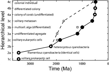
Next, fossils were assigned to a hierarchic level based on their morphology, sometimes relying on analogies with extant organisms. The time of first occurrence of each level was determined from published estimate for the stratigraphic unit in which each fossil was found. The resulting plot of hierarchical levels as a function of time is shown in Fig. 1(a). The data points show a regular increase in the hierarchical structure extending over the Precambrian and into the early Phanerozoic from ∼3500 to ∼500 Ma, all levels and sublevels arising in order. The lines are outer envelopes that document a trend in the maximum on the assumption that a hierarchical level, once achieved, was never lost. This is the best documented macroevolutionary trend observed over such a long period.

Fig. 1.

Trend in the hierarchical organization of organisms. Hierarchical levels based on nestedness (levels 1–4) and individuation (sublevels a–c). Only four levels were considered; although a few examples of aggregation at level 5 (supercolonies) are known in cyclostome bryozoans, siphonophores and ants, and level 6 might be reached by human society (McShea & Changizi Reference McShea and Changizi2003); because individuals in these aggregations are not attached to each other and difficult to detect in fossils, they were excluded (see, however, Pettersson Reference Pettersson1976). Owing to imperfect preservation and/or absence of modern analogues, some specimens could not be assigned with confidence to a single level; each was assigned either to the lowest (restrictive view, solid circles, solid line) or to the highest level in its range (permissive view, empty square and dashed line), so that for five levels two times of first occurrence were determined. The lines are outer envelopes showing the trajectories on the assumption that a hierarchical level, once achieved, was never lost. Level 1c was not included in either line, because the first known solitary prokaryotic cells slightly post-dates the first prokaryotic filaments (level 2a). (The permissive view of the data indicates four skips: 2a before 1c, 3a before 2c, 3c before 3b and 4c before 4b. Although suspicious, this view raises the possibility that hierarchical saltations may be relatively easy and that lower levels might arise as reversals from higher level organisms.) Redrawn from McShea (Reference McShea2001b).

The lines are subject to several kinds of uncertainties: on fossil dating, on assigning a level to a fossil (as shown by the difference between the two lines), possible bias in fossil preservation and the sensitivity of the maximum to sample size. Assuming that these sources of errors can be neglected, several tentative conclusions can be drawn from (the restrictive view of) the data. First, skipping of levels occurs with much lower probability than single step increases from one sublevel to the next. Second, this incremental increase is not produced by a single lineage, as most first occurrences are from representatives of different and often distantly related groups. Third, the ‘waiting time’ for transition between successive maxima tends to decrease both with time and with increasing hierarchical level.

Fourth, two opposite processes can take place in the course of evolution – aggregation or disaggregation (McShea Reference McShea2001b). For example, a solitary multicellular organism can form a colony or the members of a colony can return to a solitary existence. Thus, the observed increase in maximum hierarchical structuring can result from a higher probability of aggregation over disaggregation (‘biased changes’) or from an equal probability of both (‘unbiased changes’). In the unbiased case, a trend occurs because at the lowest level further decrease is not possible. The prokaryotic cell being the lowest level compatible with autonomous life, the global trend can be interpreted as a passive diffusion away from this lower boundary (or ‘left wall’, Gould Reference Gould1996). In the biased case, forces would be at work favouring aggregation. The biased mechanism is favoured by the fact that the transition from protists to multicellular organisms occurred several times (Bonner Reference Bonner1998), whereas no case of a reverse transition from a multicellular organism to a solitary protist or from a eukaryotic cell to a solitary bacterium is known. However, few major increases are known at the lowest levels so that a few reversals would be enough to balance numbers of increases and decreases; in the present state of knowledge, the discovery of two or three species of free-living protists having arisen from a metazoan cannot be excluded (McShea Reference McShea2001b).

Although a direct test on the major transitions is not possible, discrimination of trend mechanisms can be based on the minor transitions, i.e. changes in the degree of individuation. Marcot & McShea (Reference Marcot and McShea2007) selected 22 clades spanning at least one instance of a minor transition for which phylogenies and relevant hierarchical data were available. The 22 clades include one group of cyanobacteria, eight groups of protists and 13 groups of metazonas (bryozoans, cnidarians, arthropods and mammals). All statistical analyses based on these data failed to reject the null hypothesis of symmetrical rates of increase and decrease (measured as changes per sampled phylogenetic branch). The only exception concerns differentiation (sublevels c) for which a significant bias was found in favour of decreases, i.e. reversal from differentiated to undifferentiated. According to these results, the clear trend of increasing the hierarchical structure throughout life history could arise from diffusion away from a lower boundary.

Evolution of size and its consequences

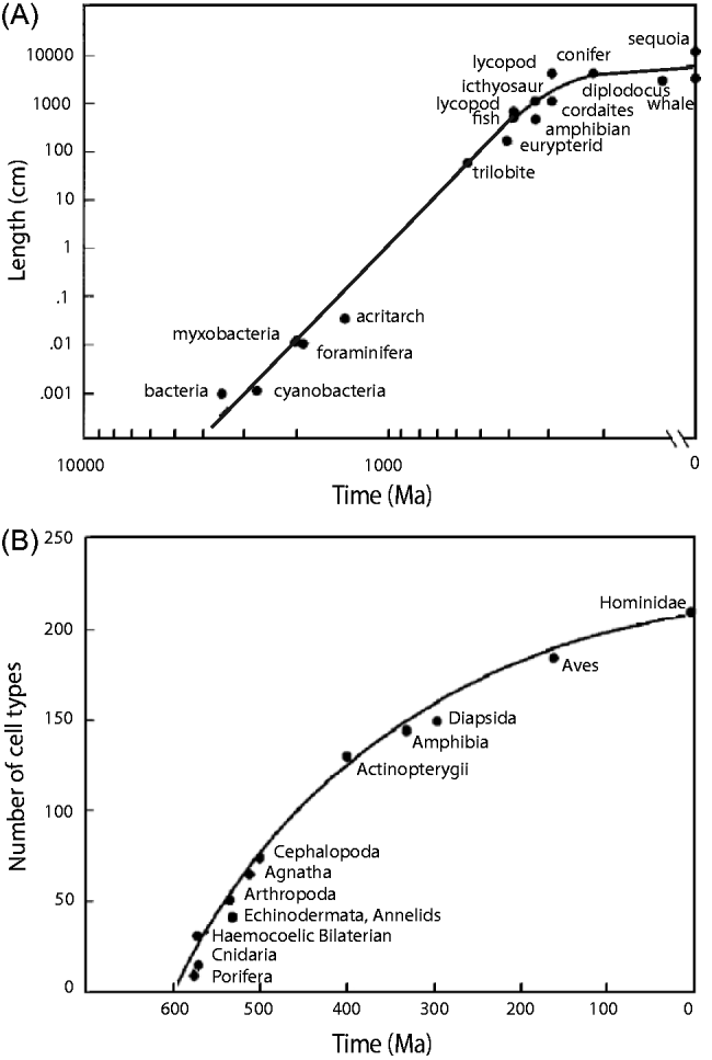
Hierarchical complexity is related to a characteristic simpler to define and measure – size. The maximum size of both animals and plants has increased progressively over geological time (Cailleux Reference Cailleux and Zeman1971, 1976; Bonner Reference Bonner1998). This is illustrated in Fig. 2(A). For example, the transition from prokaryotic to eukaryotic cells entailed a ten-fold increase in size. For Bonner (Reference Bonner2006) size is not just a by-product of evolution but a prime mover of all other changes, ‘a supreme regulator of all matters biological’ (p. 2). First, in any environment, whether an ocean, a pond or a forest, there is always an array of organisms of different sizes that are adapted to their own-sized niche. As a result of Darwinian natural selection, all size levels are filled up and if one is vacated it is soon filled. However, the largest size level is always open and available to be filled by bigger organisms to escape the competition with the smaller ones. ‘This simple fact explains why the world has evolved from one in which there was nothing larger than bacteria to today's, in which we have blue whales and giant sequoias’ (p. 65) and it is worth noting that the argument holds for any character, including ‘intelligence’. Second, any increase in size entails a number of consequences that are all rooted in physics. The strength and the weight of a limb or a branch do not vary identically when size increases: strength varies as the square of the linear dimensions and weight as the cube, so that strength varies as (weight)^2/3. The same relationship holds for diffusion that occurs through a surface, such as oxygen in lungs and nutrients in intestines. These simple relations explain why the legs of an elephant are much bigger in proportion than those of a dog, and why the internal surface of lungs, intestines and other organs folds. However, simple changes in shape are not sufficient to support a large increase in size. To get oxygen to its internal tissues, a large aerobic animal needs a circulatory system with gills or lungs, heart, capillaries etc. As size increases the demands of the surface-size rule moulds much of the shape of large organisms and dictates an enormous increase in complexity.

Fig. 2.

Size and number of cell types through time. (A) Log–log graph of the maximum sizes of organisms. (B) Estimated maximum numbers of cell types of early members of various groups. Redrawn from Bonner (Reference Bonner2006); data from Valentine et al. (Reference Valentine, Collins and Meyer1994).

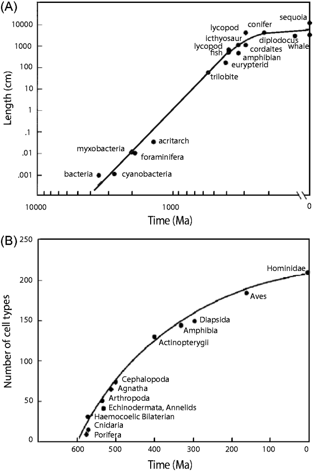
These consequences of size increase provide complementary ways to measure complexity. With some exceptions (in bacteria, protists, eggs) the size of cells and the nucleo-cytoplasmic ratio (ratio of the size of the nucleus to that of the cytoplasm) are remarkably constant in most organisms, likely as a consequence of an adequate surface–volume ratio. Thus, the easiest way to become bigger is to add more cells and then to specialize the cells. For example, the microscopic alga Volvox is a sphere of ∼50 000 cells forming a single layer. These cells belong to only two types, the numerous vegetative cells (they are photosynthetic and have two flagella that move the colony) and the reproductive cells (without flagella). Some filamentous cyanobacteria have two types of vegetative cells, the photosynthetic cells and those that fix nitrogen; they are separated because the nitrogen-fixating enzymes are inhibited by oxygen. Many more types of cells are present in large animals and plants. Therefore, the number of cell types of an organism can be considered as an indicator of the division of labour among its cells and a measure of its complexity. Rough estimates of the number of cell types and of the total number of cells in different organisms from small colonial forms to large animals and plants have been gathered by Bell & Mooers (Reference Bell and Mooers1997) and shown to be correlated in a log–log plot. Although these estimates are not accurate, because they have not been obtained with standardized protocols and consistent definition of cell types, they are nonetheless informative. Knowing that the number of cells and cell types increases with the size of organisms and that the maximum size of organisms has increased through time, it can be inferred that the maximum number of cell types must have also increased with time. This inference has been verified by Valentine et al. (Reference Valentine, Collins and Meyer1994). They plotted the number of cell types for extant species considered as representatives of their body plans against time of origin for their body plans (Fig. 2(B)). Only the specimens having the maximum number of cell types at different times were kept. McShea (Reference McShea1996) objected that the estimates for the four most recent taxa (amphibians, diapsid reptiles, birds and hominids) are probably too high because their cells have been studied much more intensively. In this interpretation, a steep increase in the maximum number of cell types would have occurred in the early Phanerozoic with little change after that. More counts will be needed to reduce the uncertainties.

Increase in size has many other effects that have been revealed by allometric studies: larger organisms move faster, they have longer generation time (Bonner Reference Bonner1965) and they live longer (Lindstedt & Calder Reference Lindstedt and Calder1981). These consequences are all significant as they favour animals that develop slowly, invest heavily in a small number of offspring (K-strategy), and rely on complex behaviours.

The increase in maximum size and maximum number of cell types must not be interpreted as an overall trend applicable to all organisms. Examples of decrease in size and in number of cell types are known (Bonner Reference Bonner2004, Reference Bonner2006). Finarelli & Flynn (Reference Finarelli and Flynn2006) used ancestral character state reconstruction to demonstrate that large body size was acquired independently in at least four terrestrial clades of caniform carnivorans, and that the body size decreased in at least one clade. It is not known whether the evolution of size is biased or unbiased. However, increase and decrease are not symmetrical events because size decrease is far less demanding than size increase. Size increase demands correlated changes in the organism, otherwise it is not viable. Size is ‘a dictator that holds complete sway over what an organism will look like and how it will function’ (Bonner Reference Bonner2006, p. 148). In contrast, size decrease may permit a decrease of strength or surfaces but it does not require it, except in extreme cases of reduction where lack of space may force to shed some of the ancestral structures.

Evolution of biodiversity

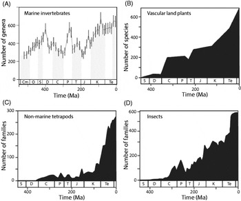
It is currently believed that all life originated from a single species. All extant organisms inherit from this species the same genetic code and molecular mechanisms for protein synthesis. The last universal common ancestor (luca) lived ∼3.5 Ma ago according to fossil and molecular evidence (Knoll Reference Knoll2003). Luca's descendents diversified through time and biodiversity increased from the initial single species to an estimated ∼10–20 million species today (May Reference May1990; Wilson Reference Wilson1992). However, the pattern of increase is still debated, as illustrated by the successive analyses of the fossil record of marine invertebrates. Analyses have focused on marine invertebrates because invertebrates are more numerous than vertebrates and preservation is more reliable in marine environments. Sepkoski (Reference Sepkoski1984, Reference Sepkoski and Walliser1996) compiled an encyclopaedic database of marine invertebrates in the fossil record based on the paleontological literature that provides the first and last known occurrences of more than 30 000 genera in ∼4000 families. The number of genera in the database plotted as a function of time, from the Cambrian explosion to the present (Fig. 3(A)), shows a steady increase during the early Cambrian. The rise apparently stopped after ∼100 Ma and was followed by a plateau for ∼200 Ma terminated by the massive late Permian extinction. After this catastrophic event, diversity recovered, then increased again up to its present level which is two times higher than the peak observed during the Paleozoic.

Fig. 3.

Trend in biodiversity of different groups expressed as number of families, genera or species plotted as a function of time. (A) Genera of marine invertebrates from the Cambrian explosion to the present (modified from Alroy et al. Reference Alroy2008). (B) Species of vascular land plants (Niklas et al. Reference Niklas, Tiffney, Knoll and Valentine1985). (C) Families of non-marine tetrapods (Benton Reference Benton1985). (D) Families of insects (Labandeira & Sepkoski Reference Labandeira and Sepkoski1993). Cm, Cambrian; O, Ordovician; S, Silurian; D, Devonian; C, Carboniferous; P, Permian; T, Triassic; J, Jurassic; K, Cretaceous; Te, Tertiary. (B–D) Modified from Benton & Emerson (Reference Benton and Emerson2007).

However, the number of genera in Sepkoski's database does not necessarily reflect actual biodiversity because paleontologists collected more and smaller fossils from young loose sediments, present in large volume, than from old hard rocks. Also, they collected, with a higher probability, the best preserved fossils and more often near their home in Europe and North America than in distant locations. Although counting genera (or families) instead of species partly correct for these defects, because genera are less difficult to count than species and their number depends less on local effort by individual paleontologists, the Meso-Cenozoic increase in diversity could be interpreted as a result of biased sampling (Raup Reference Raup1976). To address these shortcomings, Sepkoski's database was improved to take into account some of the biases in sampling and fossil preservation. In the first study, Alroy et al. (Reference Alroy2001) compared two periods of ∼150 Ma, one during the Paleozoic plateau and the other during the Meso-Cenozoic rise, and concluded that the Meso-Cenozoic rise might be an artefact. In the second study, Alroy et al. (Reference Alroy2008) extended their analysis to all periods of the last 600 Ma with refined statistical methods correcting a wrong weighing assumption of the previous work. They found that the Meso-Cenozoic rise reappears, although not as much as in Sepkoski's curve. The recent number of genera is only 30% higher than the Paleozoic peak, not two-fold higher. The authors conclude that saturation has been reached. This may indicate that the carrying capacity of the oceans, which depends on the way that energy is captured in marine ecosystems, has been reached (Sepkoski Reference Sepkoski and Walliser1996). However, critics believe that the methods used are too conservative, minimize recent biodiversity and call for a third iteration (Kerr Reference Kerr2008).

The diversity on land deserves special attention because 90±5% of all living macroscopic species are found on land. Only 5% (Benton Reference Benton2009) or 15% (May Reference May1994) of species live in oceans, although the oceans cover ∼70% of Earth's surface. The pre-eminence of terrestrial over marine diversity dates from the mid-Cretaceous period (∼110 Ma). It is ultimately related to the low cost of mobility on land resulting from physical differences between air and water in density, viscosity, specific heat and diffusion coefficient of oxygen (Vermeij & Grosberg Reference Vermeij and Grosberg2010). Life on land started primarily with cyanobacteria in the Precambrian. Multicellular organisms would have followed in the Ordovician (∼470 Ma). The earliest fossils on land are from the Silurian (425 Ma) for vascular plants and arthropods, the Devonian for tetrapods (400 Ma), trees and flying insects (375 Ma). The diversification on land has been studied in various groups from the Silurian (430 Ma) (reviewed in Benton & Emerson Reference Benton and Emerson2007), including vascular land plants (Niklas et al. Reference Niklas, Tiffney, Knoll and Valentine1985), non-marine tetrapods (Benton Reference Benton1985; Sahney et al. Reference Sahney, Benton and Ferry2010) and insects (Labandeira & Sepkoski Reference Labandeira and Sepkoski1993; Mayhew Reference Mayhew2007). The curves for the three groups are globally increasing (Fig. 3(B)–(D)). Apparently, the curve for vascular land plants presents several phases like the curve for marine invertebrates. In contrast, the curve for insects is closer to linear and that for non-marine tetrapods is exponential. These curves were not corrected for biases in sampling and preservation. Although the fossil terrestrial record is patchy and incomplete because sedimentation is more sporadic on land than in oceans, Benton (Reference Benton2010) maintains that the counts correctly reflect diversity. The evidence for geological artefacts is limited, the order of fossils in the rock is internally consistent (e.g. no mammals in Cambrian deposits was ever found) and in broad agreement with the molecular phylogenies. Moreover, fossil diversity and rock volume parallel each other, indicating that both may be controlled by a third cause, such as changing sea level. So, even if over-estimated, the observed increases in diversity seem difficult to explain by biased sampling. Overall, life on land seems to have increased exponentially and if an equilibrium level has been reached this is only recently. This is well illustrated by tetrapods (Fig. 3(C)) that increased from 1 to 27 000 species in the course of the last 400 Ma (Benton Reference Benton2010). With this exponential diversity of life, the world is increasingly divided into finer ecological niches, which means that a greater number of species offers more opportunities for the apparition of new species.

Fast diversifications, called adaptive radiations, are frequently observed, for example the diversifications of terrestrial plants in the Devonian (∼400 Ma) and of the mammalian orders during the Mesozoic. Such evolutionary success is frequently attributed to two conditions, a key innovation and an ecological opportunity. Examples of innovations are the apparition of the flower in the Cretaceous (∼110 Ma), or of echolocation for bats, the mammalian group with the largest number of species. In fact, molecular phylogenetics suggests that the notion of a single key innovation is often too restrictive and must be replaced by a whole sequence of innovations (for plants, see Donoghue 2005). The second condition for success is a corresponding evolutionary opportunity, for example the ‘empty’ Devonian land environment for plants and the habitats vacated by dinosaurs for mammals.

Five major mass extinctions took place at the end of Ordovician (440 Ma), Devonian (360 Ma), Permian (250 Ma), Trias (199 Ma) and Cretaceous (65 Ma). According to Raup (Reference Raup1991) the percentage of species that disappeared in these successive crises was 45, 25, 55, 35 and 35%, respectively. For Erwin (Reference Erwin2006), ∼95% of species died out during the Permian crisis. However, all extinctions were followed by rapid rebounds (Sepkoski Reference Sepkoski1984; Benton & Emerson Reference Benton and Emerson2007; Alroy et al. Reference Alroy2008). After most of them, the global diversity rose to levels even higher than those prior to the extinction.

Convergent evolution

A remarkable feature of evolutionary processes is the ubiquity of convergence. Convergent evolution occurs when descendants resemble each other more than their ancestors did. Classical examples of convergences are provided by marsupials. The evolution of marsupials in Australia paralleled the evolution of placental mammals in other parts of the world. There are Australian marsupials resembling mice, moles, anteaters, squirrels, cats, wolves, etc. (Simpson & Beck Reference Simpson and Beck1965; Chaline & Marchand Reference Chaline and Marchand2002). Many innovations appeared several times in widely separated lineages. For example, the transition from protists to multicellular organisms occurred at least 13 times independently (Bonner Reference Bonner1998); the camera eye appeared at least 40 times in groups as different as medusa, annelids, cephalopods, vertebrates with enough differences in detail to attest their independent apparition (Salvini-Plawen & Mayr Reference Salvini-Plawen and Mayr1977). Ants of genera Atta and Acromyrmex domesticated different fungi at least five times ∼50 Ma ago. Molecular phylogenetic studies indicate that convergent evolution may have been more frequent than thought previously. For examples, analyses revealed morphological and ecological convergences between species of lizards, from different families in Australia and North America (Melville et al. 2005) and from the same genus in Caribbean islands (Losos et al. 1998). In the latter case, ‘ecomorphs’ of different islands, undistinguishable from morphology and ecology, were shown to be the result of independent evolutionary transitions. Many more examples are documented in Conway Morris (Reference Conway Morris2003, 2010, 2011).

Evolution of brain size (encephalization)

Brains and other soft tissues are not preserved in the fossil record. Therefore, information is limited to endocranial casts (endocasts) of fossil skulls that show only the size and shape of the brain (Krubitzer & Kaas 2005). Natural endocasts form when sediment fills the endocranial cavity. Subsequent weathering removes the fossilized bone, exposing the cast. In most mammals, endocasts closely approximate brain volume (Gittleman Reference Gittleman1986). Preservation can be excellent, but the number of complete endocasts is small. Other methods hold promise to determine more endocranial volumes, computerized tomography of fossil crania (e.g. Marino et al. Reference Marino, Uhen, Pyenson and Frohlich2004) and indirect methods based on correlations of endocranial volume with better preserved parts of the skulls (Finarelli & Flynn Reference Finarelli and Flynn2007). Brain size can be measured by volume or mass as the density of brain tissue is ∼1.0 g ml⁻¹ (Marino et al. Reference Marino, Uhen, Pyenson and Frohlich2003).

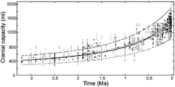
The few endocasts from mammal-like reptiles and the earliest mammals indicate that these taxa possessed relatively small brains. Apparently, brain size varied little until ∼60 Ma ago, when the major radiations of marsupial and placental mammals began (Northcutt & Kaas Reference Northcutt and Kaas1995). During 3.5 Ma of human evolution, an enormous increase in brain size has occurred, from 450 cm³ in Australopithecines to ∼1350 cm³ in modern Homo sapiens and 1500 (range 1200–1750) cm³ in extinct Homo neanderthalensis (Roth & Dicke Reference Roth and Dicke2005). Several studies provide detailed data on this trend during the last ∼3.2 Ma, for 3–8 species of extinct and extant primates from genera Cercopithecus, Paranthropus, Australopithecus, Pan and Homo (McHenry Reference McHenry1994; Kappelman Reference Kappelman1996; Rapoport Reference Rapoport1999; Falk et al. Reference Falk, Redmond, Guyer, Conroy, Recheis, Weber and Seidler2000, Reference Falk, Hildebolt, Smith, Morwood, Sutikna, Jatmiko, Saptomod and Prior2009; Elton et al. Reference Elton, Bishop and Wood2001; Leonard et al. Reference Leonard, Robertson, Snodgrass and Kuzawa2003; Neill Reference Neill2007). Lent et al. (Reference Lent, Azevedo, Andrade-Moraes and Pinto2012) included five other genera (Parapithecus, Aegyptopithecus, Proconsul, Sahelanthropus and Ardipithecus), extending the time range to ∼35 Ma ago. The most extensive report (de Miguel & Henneberg Reference de Miguel and Henneberg2001), based on more than 2161 fossil specimens of a dozen species dated from 3.2 Ma to 10 ka, shows that the trend is gradual with no apparent discontinuities (Fig. 4). The best-fit curve to the data is a double exponential function of time which explains 90% of the total variance.

Fig. 4.

Trend in hominid brain size (cranial capacity V in cm³) over 3.2 Ma based on 217 fossil adult specimens (grey points) of a dozen species, Australopithecus afarensis (⩾3200 ka), Australopithecus africanus (⩾2900), Australopithecus garhi (⩾2500), Australopithecus aethiopicus (⩾2390), Australopithecus boisei (⩾2250), Australopithecus robustus (⩾2000), Paranthropus robustus (⩾2000), Homo habilis (⩾1900), Homo erectus (⩾1800), archaic H. sapiens (⩾750), Homo heidelbergensis (⩾600), H. sapiens neanderthalensis (⩾350), H. sapiens (⩾300). The line of best fit, determined on the average capacities for each hominid fossil by date (black dots), is a double exponential function, V=306.63×4.83^x, with x=0.9995^t and t time before present expressed in ka; it explains 90% of the total variance. Most data points are included within the 99% confidence interval around this curve (dashed curves). Non-parametric testing based on the chronological rank of specimens indicates that the trend is highly significant (p=10⁻⁴). Modified from de Miguel & Henneberg (Reference de Miguel and Henneberg2001).

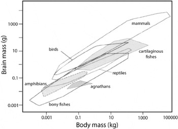
However, these studies do not take into account the relationship between brain mass and body mass – a classical example of allometric relationship. It has been shown on extant species that the magnitude y of a wide variety of anatomical and physiological phenomena, including brain size is a power function of the body size x, y=ax^b (Huxley Reference Huxley1932; Teissier Reference Teissier1936; Schmidt-Nielsen Reference Schmidt-Nielsen1984). The classical plot of brain mass as a function of body mass for species of various vertebrates, established by Jerison (Reference Jerison1973), shows, as expected from the power law, that the logarithm of the brain mass (log y) is a linear function of the logarithm of the body mass x (Fig. 5). It shows also that the slopes b but not the intercepts log a are the same for the ‘lower’ vertebrates (fishes, amphibians and reptiles) and the ‘higher’ vertebrates (birds and mammals). Thus, the points for ‘lower’ and ‘higher’ vertebrates fall approximately on two parallel lines. Slope b<1 indicates that when the body enlarges, the brain also enlarges, but not in proportion (negative allometry). Therefore, brain is the largest in the largest animals but, when measured as a percentage of body mass, is largest in the smallest animals. For example, the human brain represents 2% of its body mass but up to 10% of the body mass of shrews, the smallest mammals (Van Dongen Reference van Dongen and Nieuwenhuys1998; Roth & Dicke Reference Roth and Dicke2005). In most radiations, brain size varies approximately 10-fold, but across all vertebrate radiations slopes range from 0.21 (agnathans like lampreys) to 0.74 (mammals) and brain size varies enormously (∼30-fold) for a given body size (Northcutt Reference Northcutt2002).

Fig. 5.

Brain mass as a function of body mass for the major groups of vertebrates in a double-logarithmic graph. Each polygon encloses the data for various species of a given group. In each group, for a given body size, there is a ten-fold range in brain size. Modified from van Dongen (Reference van Dongen and Nieuwenhuys1998).

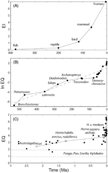
Knowing this allometric rule, it becomes possible to remove the confounding effect of body size and to investigate the evolution of brain size as if all animals had the same size. One measure of relative brain size is the deviation of a species point from the overall line characterizing the group studied – the encephalization quotient (EQ; Bauchot & Platel Reference Bauchot and Platel1972; Jerison 1973, Reference Jerison1991; Mace et al. Reference Mace, Harvey and Clutton-Brock1980). EQ can be interpreted as the amount of additional brain matter an animal has over its basic somatic needs. Traditionally, following Jerison, EQ has been considered as a measure of ‘intelligence’. It is not necessary to adopt this interpretation to find an interest in EQ measurements. Estimates of maximum EQ reached at different evolutionary times were published by Meyer (Reference Meyer1954) for 16 species of mammals over ∼70 Ma, by Russell (Reference Russell1983) on 18 fossil species over 530 Ma, and by Kappelman (Reference Kappelman1996) on 48 fossil specimens of eight species of hominids over the last 3 Ma (Fig. 6). All curves show an increasing trend with a doubling time that apparently shortens with time. As the body mass of fossils must be reconstructed for determining the EQ, the uncertainties on brain mass and body mass cumulate. Russell (Reference Russell1983) estimated the error on EQ values to be ±15% and on times to be ±2%.

Fig. 6.

Trend in maximum encephalization. (A) Mean encephalization index (EI) for five groups of vertebrates over ∼400 Ma; EI is the ratio of cerebral hemispheres over inferior brain centres (redrawn from Meyer Reference Meyer1954). (B) Encephalization quotient (EQ) for 18 fossil organisms over 530 Ma. The first three organisms (Branchiostoma, Petromyson and Latimeria) are extant and taken as representative of the maximum level of encephalization in existence for the time indicated (Paleozoic era). The 10 Cenozoic organisms are Plesiadapis, Tetonius, Heptodon, Homacodon, Necrolemur, Leontinia, Argyrocetus, Homo habilis, H. erectus and H. sapiens. The regression line (dashed) is ln EQ=0.0135×(531−t)−6.23 (redrawn from Russell Reference Russell1983). (C) EQ for 48 fossil specimens of eight hominid species (Australopithecus, squares; early Homo species, stars; archaic Homo sapiens, circles; modern H. sapiens, diamonds) over the last 3 Ma; the empty symbols are means (on time and on EQ) for each group; the two dashed lines are mean±standard deviation for extant apes (redrawn from Kappelman Reference Kappelman1996).

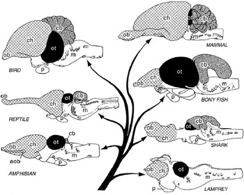
However, this trend in maximum does not imply a uniform trend for two reasons. First, six separate linear evolutionary sequences (morphoclines) have been recognized in vertebrates: (1) lampreys to hagfishes in agnathans; (2) squalomorph to galeomorph sharks in cartilaginous fishes; (3) polypteriforms to teleosts in bony fishes; (4) amphibians to reptiles; (5) reptiles to birds; and (6) reptiles to mammals (Northcutt Reference Northcutt2002). Brain size has increased independently in some members of each of these radiations (Fig. 7). As a result, many cartilaginous fishes have brains as large for their body size as those of birds and mammals. Second, in many members of each vertebrate radiation relative brain size has not increased, and it has even decreased in some members (Northcutt Reference Northcutt2002). For example, relative size decreased in lungfishes and amphibians (Roth et al. Reference Roth, Nishikawa, Naujoks-Manteuffel, Schmidt and Wake1993) whose brain and body are composed of a smaller number of bigger cells (Bonner Reference Bonner2006). In bats, relative to the ancestral state, brain size has been reduced in fast flyers, while it has increased in manoeuvrable flyers adapted to complex habitats (Safi et al. Reference Safi, Seid and Dechmann2005). The fossil hominid, Homo floresiensis, on the island of Flores in Indonesia, has a smaller brain than its putative ancestor, Homo erectus (Falk et al. Reference Falk, Hildebolt, Smith, Morwood, Sutikna, Brown, Jatmiko, Wayhu Saptomo, Brunsden and Prior2005).

Fig. 7.

Lateral views of the brains of extant species representative of the main groups of vertebrates and their phylogenetic relationship. The brains of most vertebrates possess the same number of divisions. aob, accessory olfactory bulb (cross-hatched); cb, cerebellum (stippled); ch, cerebral hemispheres (cross-hatched); m, medulla oblongata; ob, olfactory bulb (cross-hatched); ot, optic tectum (black); and p, pituitary gland. The brains are not drawn to the same scale; the variation in both overall brain size (see Fig. 5) and the size of most brain divisions is much greater than shown. From Northcutt (Reference Northcutt2002).

That brain size can be subject to bi-directional selection has been confirmed by a detailed study of caniform carnivorans (dogs, bears, skunks, otters, sea lions etc.; Finarelli & Flynn Reference Finarelli and Flynn2007). The distribution of caniform EQs remained relatively stable from 36 to 8 Ma. At ∼6 Ma, median and maximum EQs both began to increase, whereas over the whole 36 Ma period, the minimum EQ tended to decrease. If a lower bound for caniform encephalization exists and this boundary is near the ancestral caniform value, the trend of increased encephalization observed could simply be the result of random diffusion away from this bound.

Evolution of brain components

Although EQ is ‘the proper and best single number for expressing brain size in an allometric world’ (Gould Reference Gould, Falk and Gibson2001), it cannot replace a detailed analysis of brain structures because the unidimensional volumetric evolution of the brain is the result of the multidimensional evolution of its constituent parts (Thireau & Doré Reference Thireau and Doré2002, Reference Thireau and Doré2003). As fossil endocasts provide information only on overall brain size and features visible on their surface, more detailed investigations must rely on living species and tentative brain reconstruction of extinct species. The evolution of three types of brain components at increasingly finer resolutions (divisions, neural centres and neurons) has been analysed.

Number and size of neural centres

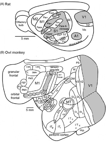
Increases in brain size have frequently resulted in increases in the number of neural centres and the number of neuronal cell classes within a centre. This is best illustrated in the mammalian neocortex (Fig. 8). In all living mammals, the neocortex is a multilayered sheet 1–3 mm thick made of a patchwork of discrete areas. The same cell density and the same basic set of primary sensory projections are found across all mammals, so the changes concern the overall surface area, the number of neurons, and the number and size of cortical modules (Rakic Reference Rakic1995; Nishikawa Reference Nishikawa1997). The more easily identified neocortical centres are sensory fields. Most investigated mammals appear to have primary (V1) and secondary (V2) visual areas, a somatosensory region with a primary area (S1) and three or four adjoining areas, a primary motor area (M1), a primary auditory region (A1) with possibly one or more additional fields. The neocortex of the first mammals was probably close to the neocortex of extant rodents (Fig. 8(A)) and contained relatively few areas, on the order of 10–20, including the sensory fields mentioned.

Fig. 8.

Organization of the mammalian neocortex in rats (A) and owl monkeys (B). The owl monkey cortex has been flattened so that hidden areas can be shown. The primary sensory areas, visual (V1), auditory (A1) and somatosensory (S1 in rat, 3b in monkey) are shown in grey. In rats, the neocortex is small and a small number of cortical areas are identified. In owl monkeys, the cortical sheet is greatly expanded and many more areas are present. Despite differences in size and number of areas, homologous areas conserve their relative positions in both species. Modified from Kaas (Reference Kaas2008).

Comparison of the homologous cortical areas identified in rats and owl monkeys shows that several areas (>50% surface) in monkey brains are absent in rat brains (Northcutt & Kaas Reference Northcutt and Kaas1995; Kaas Reference Kaas2008). In visual cortex alone, the number of functional subdivisions is 3–8 in rats, >20 in owl monkeys and >32 in macaques. This increase in the number of functional subdivisions has occurred independently numerous times among mammals.

Various parts of the neocortex are relatively much larger in humans than in chimpanzees, in particular the thumb and finger areas of the motor cortex that are related to manual dexterity, and the Wernicke's and Brocas's areas that are related to verbal communication (Northcutt & Kaas Reference Northcutt and Kaas1995).

Energy constraints

All electric signals in neurons are created by the opening of channels selectively permeable to sodium, potassium and other small ions. The resulting passive ionic movements depolarize the neuron membrane yielding local post-synaptic potentials in dendrites and propagated action potentials in axons. These ion movements are compensated by active, energy consuming processes. Most of the energy in nervous tissues serves to drive the sodium–potassium pumps that maintain constant the concentrations of sodium and potassium ions. The brain is an energetically very expensive organ that demands a large and continual supply of glucose and oxygen irrespective of whether the animal is awake or asleep, active or at rest. For example, the human brain, only 2% of body mass, consumes ∼20% of the total energy at rest (basal metabolism). The energy constraints on brain help to understand several features of brain evolution.

The increase in body and brain sizes implies greater neuron number and axon length, especially to communicate between cerebral areas. For example, in the mammalian neocortex, the volume of the white matter that contains long axons increases faster than the volume of the gray matter that contains cell bodies, dendrites and short axons for local information processing (b=1.47; Zhang & Sejnowski Reference Zhang and Sejnowski2000). In order to decrease axonal energy consumption and increase conduction speed, long segments of insulating myelin sheath are wrapped around the axons that limit ionic movements to interval between segments (nodes) resulting in saltatory conduction of action potentials from one node to the next. The myelin sheath, made of tight helically wound glial membrane, have arisen independently several times in vertebrates, annelids and crustaceans (Hartline & Colman Reference Hartline and Colman2007).

Heart, liver, kidney and the gastrointestinal tract are also ‘expensive’ organs that consume ∼50% of basal metabolism of the human body. An increase in brain size can be balanced by a reduction of these organs (‘expensive tissue hypothesis’, Aiello & Wheeler Reference Aiello and Wheeler1995). In the case of the human brain, the reduction of gut size had to be compensated by an increase in the quality of food (Aiello et al. Reference Aiello, Bates, Joffe, Falk and Gibson2001; Roth & Dicke Reference Roth and Dicke2005). Brain size and diet quality are positively correlated in most living primates and they changed together in their evolutionary history (Fish & Lockwood Reference Fish and Lockwood2003). The fast growth of the human brain in prenatal and first post-natal years is especially demanding for both mother and infant (Aiello et al. Reference Aiello, Bates, Joffe, Falk and Gibson2001; ‘maternal energy hypothesis’, Martin Reference Martin1996).

Another solution to the energy problem of producing and maintaining a brain is to reduce its size. Bats foraging in open space have small and narrow wings relative to body mass rendering them efficient flyers but poorly manoeuvrable, while the opposite is true for species foraging in complex environments. Relative to the ancestral state, brain size in bats has been reduced in fast flyers, while it has increased independently several times in agile flyers. These opposite evolutions correspond to two types of foraging. Fast flying bats are aerial insectivores which hunt by echolocation whereas agile bats must find energy rich food at locations unpredictable in time and space, and searching requires large brains (Eisenberg & Wilson Reference Eisenberg and Wilson1978; Mace et al. Reference Mace, Harvey and Clutton-Brock1980; Safi et al. Reference Safi, Seid and Dechmann2005).

Convergences

Several examples of convergences in brain evolution were mentioned above. Cladistics has revolutionized our understanding of brain evolution by demonstrating that many brain structures, traditionally thought to be homologous, had in fact evolved several times independently in taxa whose common ancestors lacked these structures. It appears now that convergence is very frequent. Relatively few cortical areas appear to be homologous among all living species of mammals. Most of the non-primary cortical areas probably expanded independently among different lineages. For example, the neurons of the middle temporal (MT) area receive input from visual areas V1 and V2 and analyse the direction of movement (not colour). The MT area is present in all investigated primates and absent in all non-primates (Krubitzer, 2009). However, an MT-like area has been found in cats and in some members of the archontan radiation (which includes tree shrews, flying lemurs and bats), suggesting that they may have arisen independently in these taxa.

Many other examples concerning neural circuits are known. Hagfishes have independently evolved a highly laminated cerebral cortex, comparable in many ways to the cerebral cortex of mammals (Northcutt Reference Northcutt2002). Similar (but not identical) circuits have evolved convergently in at least four frog lineages controlling precise coordination of tongue and jaw movements during prey capture and illustrate how small changes in neural pathways can lead to dramatic changes in an organism's abilities (Nishikawa Reference Nishikawa1997, Reference Nishikawa2002). In electric fish that generate an electric field to sense their environment, jamming avoidance evolved independently in African and American fishes. This solution to avoid interference between the signals emitted by two individuals at close proximity was acquired through relatively small changes in the physiology (neurotransmitters, membrane properties) and interconnections of neurons used previously for a different purpose (Nishikawa Reference Nishikawa1997). An example of more global significance is parallel distributed processing and population coding in neural networks that have evolved convergently in distantly related species throughout the animal kingdom (Nishikawa Reference Nishikawa1997; Heinze & Homberg Reference Heinze and Homberg2007).

Evolutionary trends in behaviour

A suggestive illustration is provided by Cailleux (Reference Cailleux and Zeman1971). He proposed a semi-quantitative method based on behavioral tests (simple reaction, T choice, labyrinth, detour, etc.). He asked two specialists of animal behaviour to list and rank these tests in order of increasing difficulty. He found the two independent scales to be in good agreement, ranging from simple directed response (level 1) to the notion of far future (level 55, end of scale). He plotted the various grades of behavioural performance of species or group of species versus their time of apparition. He found that successive equal levels were crossed in exponentially shorter times (see Fig. 2 in Rospars Reference Rospars2010). Although suggestive, this approach suffers from the obvious limitation that the behavioural scale is partly subjective and does not provide proof of the equivalence of equal intervals (is the jump from level 1 to level 11 equivalent to the jump from 21 to 31?).

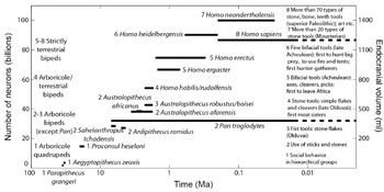
Lent et al. (Reference Lent, Azevedo, Andrade-Moraes and Pinto2012) illustrate a similar approach in human ancestors which links brain volume, number of cerebral neurons, main motor behaviours and cognitive achievements (Fig. 9). However, the link remains qualitative as the motor and cognitive scales are qualitative. Clearly, before cognitive trends can be studied, quantitative scales of cognition have to be established.

Fig. 9.

Trend in the number of neurons in human ancestors (left axis) derived from endocranial volumes (right axis). The derivation is based on the isometric scaling law between brain volume and number of neurons in primates (Herculano-Houzel et al. Reference Herculano-Houzel2007, Reference Herculano-Houzel2011). Ancestral primates had less than 20 billion neurons, Australopithecus, had ∼40 billion neurons, just above the chimpanzees (∼30 billion neurons). In the genus Homo, the number of neurons grew from ∼50 billion (H. habilis) to ∼70 (H. erectus) and finally ∼90 (H. sapiens) and even ∼100 (H. neanderthalensis). The 15 species are numbered according to eight cognitive levels (on the right) and four motor behaviours (on the left). Redrawn from Lent et al. (Reference Lent, Azevedo, Andrade-Moraes and Pinto2012).

Relationship between intelligence and brain

Any brain is a compromise between costs and benefits. We have analysed energetic costs, what are the benefits? The main advantage hypothesized or even assumed of big brains is ‘intelligence’. This raises three questions: how to measure intelligence? Does intelligence facilitate the survival and/or reproduction of animals in the wild? How is intelligence related to brain?

Is behavioural flexibility related to brain features?

The previous studies provide the behavioural data whose absence prevented for so long a quantitative answer to this essential question. Lefebvre et al. (Reference Lefebvre, Whittle, Lascaris and Finkelstein1997) used the ratio of forebrain volume (the equivalent of cortex in birds) over brainstem volume (medulla, pons and midbrain) and found that it was significantly related to both absolute and relative innovation frequency per order. Reader & Laland (Reference Reader and Laland2002) used three measures of brain size: the ‘executive brain’ volume (calculated as the sum of neocortex and striatum volumes), the ‘executive brain ratio’ (executive brain volume over brainstem volume, equivalent to EQ because brain stem volume is well correlated to body mass), and residual executive brain volume, calculated by including brainstem in a multiple regression. All three measures of behavioural flexibility (innovation, social learning and tool use frequencies) were found to be significantly positively correlated with executive brain volume and executive brain ratio (but not with residual executive brain volume). These findings support the view that multiple factors have been important in the evolution of large brains, involving technical skills, as well as social and ecological factors, since most innovations are foraging innovations. However, these studies of birds and primates do not establish whether increased forebrain or neocortex size was directly selected because these brain regions facilitates complex behaviours, or if the improved information processing capacities resulting from an increase of these regions was used secondarily to cope in new ways with environmental challenges.

Other characteristics than innovation frequency and tool use are positively correlated with relative size of the brain or brain components (Morand-Ferron et al. Reference Morand-Ferron, Sol and Lefebvre2007) – learning speed, capture of mobile prey, group size and/or social complexity, frugivory and kleptoparasitism, that is, the stealing of food items already procured by others. Collectively, they provide strong evidence that the cognitive skills of animals are limited by the size of the brain.

Deaner et al. (Reference Deaner, Isler, Burkart and van Schaik2007) studied the correlations between eight neuroanatomical measures and their quantitative estimate of global cognition for 24 non-human primate genera (see above). They found no significant correlation with measures based on EQ or brain size residuals that control for a possible effect of body size. The best two predictors of global cognitive ability were the logarithms of whole brain size and of neocortex size. These results call into question the hypothesis that the primate brain can be divided into somatic and cognitive parts and the usefulness of EQ in cognitive studies. They also provide an objective basis to convert the trend in brain size shown in Fig. 9 into a trend in global cognition.

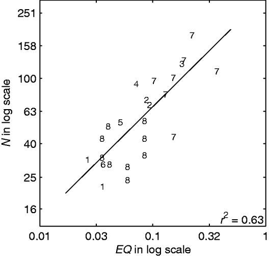
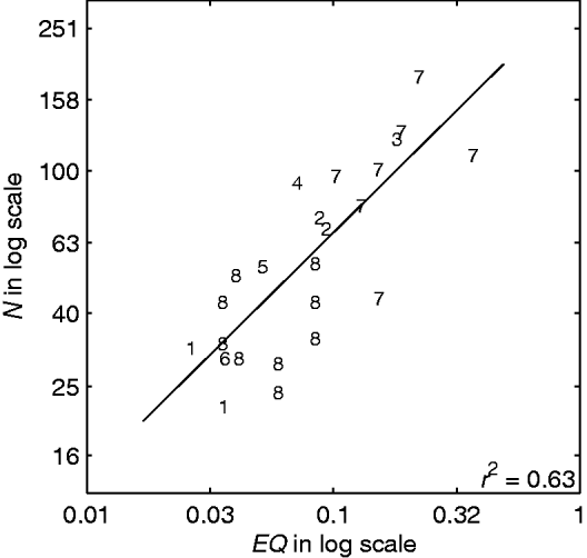
Changizi (Reference Changizi2003) showed in mammalian species from eight orders that behavioural repertoire size – the number of unique categories of behaviours displayed by a species – is significantly correlated with encephalization (Fig. 10). Although ethologists may have difficulties for delineating and counting behaviours (grooming, sitting, jumping, scratching ears, etc.), ethogram size appears as an informative measure related to behavioural flexibility. Further work in this direction is desirable as this measure holds the promise to be applicable across a wider array of species than other methods.

Fig. 10.

Number of behaviour types as a function of encephalization index in mammals. Behavioural repertoire size (N) as determined by ethologists and encephalization index (EQ) defined as brain size after correcting for body size. Each point represents a different species (or a mean value for several species) from eight orders: Artiodactyla (1), Carnivora (2), Cetacea (3), Chiroptera (4), Insectivora (5), Lagomorpha (6), Primates (7) and Rodentia (8). Regression line of N on EQ is shown. Data from Table 1 in Changizi (Reference Changizi2003).

Evidence for non-human ‘high intelligence’

It has long been thought that tool use, tool-making, syntactical-grammatical language, self-awareness, imitation, deception and ‘theory of mind’, that is, the ability to understand another individual's mental state and to take it into account in one's own behaviour, were unique properties of humans that required an exceptionally large brain. Both views have been undermined. A major contribution of ethology and animal psychology has been to demonstrate that man's abilities are not so unique. Although signs of imitation, theory of mind and syntactical language were found in non-human animals, the evidence is still debated (Roth & Dicke Reference Roth and Dicke2005), but the other signs of ‘high intelligence’ are better established. Deception has been widely observed among monkeys (Bates & Byrne Reference Bates and Byrne2007). Tool use, defined as ‘the use of an external object as a functional extension of mouth, beak, hand, or claw, in the attainment of an immediate goal’ (van Lawick-Goodall Reference van Lawick-Goodall1970) has been observed in many primates, birds and other animals. For example, New Caledonian crows can craft hook tools that are used to poke out insect larvae from holes in trees and acquire otherwise unobtainable foods (Hunt Reference Hunt1996).

The understanding that one's own mirror reflection does not represent another individual but oneself appears in humans at 18–24 months of age and marks the beginning of self-awareness. Until recently it was known only in great apes (Gallup Reference Gallup1970). Monkeys, other non-primate mammals and several bird species typically respond to a mirror by social behaviours, e.g. aggressive displays, quickly followed by disinterest. In a few ape species (chimpanzees, bonobos, orang-utans, some of gibbons and gorilla), however, behaviour changes over repeated presentations with a mirror. Social behaviour decreases and the mirror is used for exploration of the own body. Behaviours suggestive of self-recognition are observed in 75% of young adult chimpanzees.

Attempts at demonstrating self-recognition in other primates and non-primates failed to provide convincing evidence, until two bottlenose dolphins were tested (Reiss & Marino Reference Reiss and Marino2001). Each dolphin studied was marked on its body with black ink and these marks were not visible to it without the use of a mirror. The subjects showed no social behaviours but engaged in mark-directed behaviours at mirrors and spent a significantly greater cumulative amount of time at mirrors when marked than when sham-marked (i.e. when a water-filled marker was used). The main difference with chimpanzees is that dolphins did not attend to marks on companions, maybe because, unlike primates, they do not groom each other. Experiments with Asian elephants gave similar results. None of the elephants aimed social behaviour at the mirror. All, like the apes and dolphins, exhibited exploratory and mirror-testing behaviour before more explicitly self-directed activities (Plotnik et al. Reference Plotnik, de Waal and Reiss2006). Finally, corvids were also tested and the European Magpie Pica pica was confronted with mirrors. The first time, the birds displayed similar sequences of behaviour as described in apes. Clear evidence for mirror-recognition was obtained in two of the five birds tested (Prior et al. Reference Prior, Schwarz and Güntürkün2008). Emery & Clayton (Reference Emery and Clayton2004) suggest that complex cognition is based on four non-verbal cognitive ‘tools’ (causal reasoning, flexibility, imagination and prospection) that are shared by both apes and corvids. These findings show that elaborate cognitive skills arose independently in two vertebrate classes, birds and mammals that diverged ∼300 Ma ago. ‘High intelligence’ appears also as a convergent feature of evolution.

Is a big brain needed to be ‘intelligent’?

This question arises because the brain of corvid birds is relatively small (∼10 g). However, it can achieve many of the cognitive operations of apes, like tool making, tool use and self-recognition. Certainly, the crow has a large brain with respect to its body as shown by its EQ which is equal to that of chimpanzees (Jerison Reference Jerison1973), but this is not a sufficient explanation. Its small absolute brain size may be compensated in part by smaller neurons and higher neuronal density (Roth & Dicke Reference Roth and Dicke2005). Unfortunately, number of neurons in corvid brains is not known. Also, the relative size of the forebrain of crows (and parrots) is significantly larger than in other birds, particularly the areas thought to be analogous to the mammalian prefrontal cortex (Reiner et al. Reference Reiner, Perkel, Bruce, Butler, Csillag, Kuenzel, Medina, Paxinos, Smimizu and Striedter2004). However, the evolution of these brain divisions has been divergent in mammals and birds; the ape neocortex is laminar, whereas the corvid nidopallium presents a nuclear organization. This gives evidence that a convergent cognitive evolution can be built on a divergent brain evolution (Emery & Clayton Reference Emery and Clayton2004). A neocortex is not a prerequisite for complex cognition.

A confirmation that the relationships between brain and cognition are intriguing and ill-understood is found in insects. Their cognitive functions have been well studied, especially in honeybee workers, and they far exceed simple hard-wired responses to specific configurations of sensory stimuli (Giurfa Reference Giurfa2003). Yet, insects have very small brains. The 1.1 mg brain of honey bees (Strausfeld 1976) contains slightly less than 10⁶ neurons. However, this is sufficient not only to provide them with sophisticated sensory systems, well-developed learning and memory capacities, some counting abilities (Gross et al. Reference Gross, Pahl, Si, Zhu, Tautz and Zhang2009), but also to endow them with the capacity to manipulate abstract notions (Chittka & Niven Reference Chittka and Niven2009). For example, bees have been trained to distinguish horizontal and vertical bands in a series of distinct patterns. When confronted with different patterns, they were able to transfer the learned discrimination and thus to generalize the first examples. Similarly, bees can learn the concept of above/below. They have also been shown to learn the notions of symmetry and similarity and, simultaneously, of asymmetry and difference. Recently, they have been shown to master simultaneously a spatial concept (above/below and right/left) and a difference concept (same/different) (Avarguès-Weber et al. Reference Avarguès-Weber, Dyer, Combe and Giurfa2012). All these cognitive tools are useful for flower recognition and navigation. Chittka & Niven (Reference Chittka and Niven2009) conclude that brain size is less related to cognitive capacity than generally assumed. They argue that a greater neuron number adds precision to perception and motor control and enlarges memory capacity, which is important for flexible behaviours, but is not necessary for qualitative shifts in behaviour.

These observations make clear that brains are intrinsically multidimensional objects. Intelligence also is multidimensional. Any attempt to reduce their multiple dimensions to a single one (brain size, EQ, number of neurons, etc.) is helpful but inevitably creates exceptions, especially when evolutionary distant brains, possibly built on different principles, are compared.

Main properties of observed trends

A trend is not necessarily indicative of a progress. All biologists have admitted till the 1960s or 1970s that a ‘progress’ had taken place during evolution because they believed that a steady increase in complexity was obvious. The notion of evolutionary progress has been criticized as loaded with value judgment. Whether the apparition of intelligence is a ‘progress’, can be debated. However, the notion was defended by Ayala (Reference Ayala and Nitecki1988) because once a standard of progress has been chosen, decisions concerning whether progress has occurred can be made following the usual methods of science.

Trends are not a modern version of the long-abandoned misconception that all beings can be arranged in a linear progressive series – the chain of being, or scala naturae – as first advocated by Buffon, Goethe and Oken. Later, this series was termed the ‘phylogenetic scale’ and led, for example, to the telecencephalization theory in which the telencephalon (cerebral hemispheres and related structures) of living adult vertebrates was seen as representing the various stages of a unilinear increase in complexity. It is now realized that evolution is better described as a ‘bush’ than as a ‘scale’ or ‘ladder’ (Parent & Hazrati Reference Parent and Hazrati1994) because all living species are the terminal results of distinct branches (clades) that have evolved independently after their divergence. As a result, organisms are mosaics of components with different rates of evolution that cannot be ranked by increasing anatomical or functional complexity (Hodos & Campbell Reference Hodos and Campbell1969; Campbell & Hodos Reference Campbell and Hodos1991). A simple organism is not ‘lower’ than a complicated one (Cailleux Reference Cailleux and Zeman1971), both may be equally fitted to their environment and, if contemporary, have evolved during the same time.

The trends observed do not give any evidence for the existence of some universal force acting on all living forms that would drive them uniformly towards higher complexity with time. The absence of overall trend presents two complementary aspects: (i) for a given characteristic not all lineages in a group show the same trend (brain size can increase or decrease) and (ii) for a given lineage, not all characteristics show the same trend (in primates, while cerebrum increases, olfactory bulb and digestive system decrease). In all examples reviewed here, different lineages showed different trends characterized by an increase, a stagnation or a decrease in complexity. Prokaryotes have not disappeared after the advent of eukaryotes, if only because bacteria are indispensable for the global functioning of the Earth ecosystem. The observed diversity of trends raises the question of whether, when a large sample of lineages of a given group is considered, the number of increases in complexity exceeds the number of decreases (biased changes). Although important for a proper understanding of evolutionary processes, a definite answer to this question is not essential for the present discussion. Biased changes do not seem necessary for the apparition of highly complex organisms. A few positive trends in different lineages appearing successively in time are a sufficient condition, especially if these lineages are evolutionary successful.

Many other variables than those chosen here might have been examined – means of reproduction, of locomotion, of nutrition, to name only a few – that might have lead to different ranking of species. Lineweaver (Reference Lineweaver, Seckbach and Walsh2008) notes that if relative nose size was chosen instead of relative brain size, elephants would be on top. Similarly, McShea (Reference McShea1996) remarks that if the human brain is ‘extraordinarily complex, in some sense and at some scale’, this may be expected from any hypertrophied and specialized structure, for example the arborescent tentacles of sabellid annelids that are more complex than those of other annelids. So, ‘with all specializations taken into account, it is not at all obvious that humans are more complex than other species’ and the higher complexity of humans ‘is not warranted by any reliable evidence’. Although provocative the objection is judicious; it is an aspect of the difficulty to compare rigorously different species and calls for further quantitative studies. The fact that, for example, the insect Locusta migratoria has almost the same number of muscles (296) than primates (316) and more than rodents (214) encourages caution (Changizi Reference Changizi2003; Chittka & Niven Reference Chittka and Niven2009). However, these remarks are misleading. The question addressed here is not to decide whether humans are more complex than other species. In a discussion of complex intelligent life it is merely more appropriate to study brain size rather than nose size and to give more weight to neural information processing than to mouth appendages. In short, complexity per se is not relevant.

The time range over which an increasing trend of a given characteristic can be observed, in a single lineage or in a wide group of lineages, is usually limited. The size of the largest animals (limited by mechanical forces) and the biodiversity of oceans (possibly limited by its carrying capacity) are examples of sigmoid trends apparently ending in a stasis. Another example of greater theoretical significance is the slowing down of the number of higher taxonomic levels with time. The mean doubling time of the number of genera was much shorter in the first half of existence of several groups than in their second half: 40 Ma in the first half then 250 Ma in the second half for fish, 25 then 100 for terrestrial tetrapods, 15 then 21 for birds and 60 then 100 for terrestrial plants (Cailleux Reference Cailleux and Zeman1971). The same slowing down, known for a long time, occurred for orders, classes and phyla. The number of phyla has increased by 2 or 3 units only in the last 500 Ma. The diversification of the living world through time has concerned first the overall body plans then the details. The hierarchical organization in time is apparently a general feature of evolution. It is observed also in the evolution of the brain and brain divisions, and likely finds its origin in developmental constraints. However, in the course of evolution, the stasis of the ‘old’ variables is taken over by ‘new’ variables, expanding complexity in other directions, at least in some lineages. Each innovation creates a set of new possibilities for qualitatively different forms of changes. So, positive trends seem to be associated with radiations, when a combinatorial explosion is made possible by innovations.

Depending on the studied variables various functions of times have been reported to describe trends – linear, exponential, logistic, hyperbolic and others. However, logarithmic transformation, applied either to the time-dependent variables (Russell Reference Russell1983) or to time (Cailleux Reference Cailleux and Zeman1971; Pettersson Reference Pettersson1976), has been the most frequently used to linearize the curves. Using the later transformation, Cailleux (Reference Cailleux and Zeman1971) and Pettersson (Reference Pettersson1976) showed that the anatomical and behavioural evolution, as well as the technical and social evolution in human societies, have accelerated through time (increasing growth rates with equal increments in exponentially shorter times). However, some evolutions, illustrated by the growth of the human population, are better described by hyperbolic functions that end as vertical asymptotes (Meyer & Vallée Reference Meyer and Vallée1975). According to the interpretation of Chaline et al. (Reference Chaline, Nottale and Grou2009), based on non-linear dynamics and punctuated equilibria, the accelerated evolutions result from a series of discontinuous innovations (index i) that appear with higher probability at successive times t _i according to a log-periodic function t _i=t _c+(t ₀−t _c)g ⁻ⁱ, where t _c is the critical time of the series and g a constant (scale factor). This function has been applied to the evolution of various clades, including the five successive cranial morphologies of primates (Dambricourt-Malassé et al. Reference Dambricourt Malassé, Deshayes, Marchand, Magniez-Jannin and Chaline1999). The critical time may correspond in this case with the apparition of H. sapiens (Chaline et al. Reference Chaline, Nottale and Grou1999). Although these independent studies support the idea that recent evolution is hyperexponential and suggest that innovations are cumulative, further research is needed to clarify and unify them. These quantitative studies are essential to model evolutionary trends and test hypotheses on their origin, notably the random diffusion hypothesis and the zero-force evolutionary law (McShea & Brandon Reference McShea and Brandon2010; Bogonovich Reference Bogonovich2011).

Are evolutionary trends repeatable?

The problem of repeatability of life on Earth, assuming the same initial conditions and the same planetary environment can serve as a simplified case before considering what could happen on different planets. If the tape of life were replayed, in what fraction of many independent repetitions will species with high intelligence appear? Many biologists have proposed pessimistic estimates: ‘vanishingly small’ (Simpson Reference Simpson1964), ‘infinitely improbable’ (Monod Reference Monod1970), ‘incredibly improbable’ (Mayr 1985), the ‘immense majority’ of repetitions will not produce a conscious being (Gould Reference Gould1996). Although dissenting views have also been expressed (e.g. Sagan Reference Sagan1995; de Duve Reference de Duve1998; Conway Morris, 2011), so that no consensus has been reached in the last 50 years or so, it is appropriate to take the pessimistic estimates as reference. Five main arguments have been proposed to support extremely small probability.

First, evolution shows no uniform trend. Evolution is not repeatable because ‘there is no central line leading steadily, in a goal-directed way, from a protozoan to man’ (Simpson Reference Simpson1964).

Counter-argument: This hypothesis of a global tendency for progress, now fallen in disrepute (Gould Reference Gould1996), is unnecessarily strong. There is no evidence that the minimal ‘random diffusion’ hypothesis for trends would not lead to their repetition.

Second, exact repetitions are impossible. Evolution depends on many fortuitous events, both in reproduction (mutation and recombination are stochastic processes) and in the environment. ‘If the causal chain had been different, Homo sapiens would not exist.’ (Simpson Reference Simpson1964).

Counter-argument: This argument proves convincingly that exact repetitions are impossible but does not rule out approximate repetitions. Recognizing the existence of alternative evolutionary paths is not sufficient to exclude that some of these paths can lead to some form of high intelligence. If history had been different and if all known favourable events had never happened, then other events would have occurred and some of them might have been favourable. No sure conclusion can be drawn from the singularity of history and a probability cannot be calculated on this basis.

Third, the number of paths leading to high intelligence is small and contingent events can prevent evolution from following them. This central argument is supported by several observations. At least 40 different phyla of animals originated in the Cambrian explosion. Many of them were quickly eliminated (possibly at random) and only one, that of chordates, eventually gave rise to ‘genuine intelligence’. If this phylum would have been eliminated this form of intelligence would not have appeared (Mayr Reference Mayr and Regis1983; Gould Reference Gould1989). Similarly, without the end Cretaceous extinction that wiped out the dinosaurs, mammals and primates would not have diversified.

Counter-argument: Although contingency certainly decreases the probability of similar repetitions, the eliminated alternative evolutionary paths might have been equally or more favourable paths for the apparition of intelligence. For example, the mammalian reptiles with their bipedal walk, thumb-like finger, frontal eyes and enlarged cerebral hemispheres might have led to highly intelligent beings with reptilian reproduction (Russell Reference Russell and Billingham1979). Is the number of solutions to develop a brain providing high flexibility and creativity large or small? It is difficult to answer this question in the present state of knowledge, although the diversity of solutions observed (insects, cephalopods, birds, primates, etc.) suggests but does not prove that this number is relatively large. The greater the number of possible paths to a given level, the higher is the probability that it is reached. The argument that bacteria are the dominant form of life on Earth, not mammals and still less human, is another form of this argument (Gould 1996). Similarly, the dominant forms of metazoan life are insects, the body plan of which are not compatible with large size and large brain, and therefore could not support human-like intelligence. The weight of this argument is difficult to assess because acknowledging that bacteria-like (or insect-like) organisms will be found in most or all repetitions does not prove that man-like beings will almost never be found.

Fourth, the paths leading to high intelligence have slow evolutionary rates. In this interpretation of the failure of repetitions the favourable paths are not necessarily rare but their evolutionary rates are very slow or null. Along many paths further development would be prevented at some point or would evolve at too low rates to give birth to highly complex metazoans during the ∼10 Ga of the stable circumsolar habitable zone.

Counter-argument: On the one hand, admittedly, lines of slow evolution and dead ends have been frequent, likely even more frequent than innovative paths. Lethal mutations and short-lived lineages leave no trace in the fossil record. One can imagine cells that cannot aggregate, or could aggregate but not support the development of multiple organs, or would lead to animals but with no possibility to evolve complex brains. It is easy to imagine oceans where the ‘highest’ life forms are very slowly evolving dolphin-like animals (Lineweaver Reference Lineweaver, Seckbach and Walsh2008).

On the other hand, it is equally difficult to identify clear biological obstacles preventing lineages to evolve at the rates actually observed. It seems likely that physical and chemical processes are dominant in the early phases of life. All chemical processes on which terrestrial life is based, including amino acids, nucleic acids, the cellular organization and even the genetic code (Freeland et al. Reference Freeland, Knight, Landweber and Hurst2000) may be universal because they depend on universal laws (de Duve Reference de Duve1998; Rospars Reference Rospars2010). Under these conditions, it is expected that the mutation rates would be similar as would the diversity of observed evolution rates. For all variables examined here that describe important features for the apparition of high intelligence, positive trends have been found; this general property suggests that the hypothesized stasis is not the rule.

Slow evolution might also result from more frequent or more severe catastrophes than in the actual Earth history, possibly resulting from the coincidence in time of several factors and destroying all life (Erwin Reference Erwin2006). Raup (Reference Raup1991) estimated that severe catastrophes would have a periodicity greater than 2 Ga. This estimate indicates that actual life may have been lucky but not extremely lucky. Conversely, the idea that a world with less frequent catastrophes would evolve more slowly can be advocated (Conway Morris 2011).

Fifth, convergent evolution of high intelligence is improbable. Convergences have been presented as evidence for repeatability (Conway Morris, 2003, 2010). However, Lineweaver (Reference Lineweaver, Seckbach and Walsh2008) pointed out that all convergent species shared a long common history before they diverged and that the extent of convergence cannot be larger than the extent of divergence from the common ancestor. For the species which converged on eyes, the divergence could only take place during the relatively brief fraction of their existence as independent organisms.

Counter-argument: Clearly, new structures must evolve from pre-existing structures. Any brain presupposes the existence of a nervous system. However, this objection must not be overstated because if historical (contingent) constraints play a role, biophysical constraints cannot be ignored. Biophysical constraints play a dominant role to mould the shape and organization of animals as illustrated previously by the ubiquitous allometric relationships, the consequences of size increase, the lesser mobility in water than on land, brain energetics, etc. Optimum solutions for swimming, walking or flying are not so many. Sensory organs are constrained by the physical nature of stimuli on the sensor side and the processing of raw sensory signals on the neural side. These constraints are the major determinant of the convergences and contingency can play only a secondary role. Constraints explain the most general features of animals, like bilateral symmetry and the presence of a head housing a brain at close proximity of many cephalic sensory organs. There is little doubt that eyes are useful in the Earth environment. They can be expected to arise with similar organizations in any repetition of the evolutionary experiment where the coordinated growth of specialized cell types is possible, even if it is now known that eyes in different phyla have evolved by means of very similar changes in the same developmental genes (Shubin et al. Reference Shubin, Tabin and Carroll2009). It is difficult to imagine solutions very different from nervous systems to conduct and process information. Even if many designs are conceivable, general principles resulting in glomeruli, retinotopic maps, population coding etc., can be expected that owe little to history and much to optimization. Although the genetic background inherited from their common ancestor channels the evolution of convergent species (Losos Reference Losos2011), in some convergences like placental and marsupial wolves, the morphologies reached are so similar that they seem to go much beyond this channelling. Convergences suggest that the possible solutions are not so many and that they can be reached repeatedly through many different paths (Conway Morris Reference Conway Morris2003, 2010).

Mayr (1985) confirms that highly complicated organs like eyes ‘can evolve repeatedly and convergently when advantageous’ but adds ‘provided such evolution is at all probable’. This restriction is important because eyes are probable, as indicated by the fact that it evolved several times, but not ‘genuine intelligence’ that evolved only once. Lineweaver (Reference Lineweaver2005) gives a vivid illustration of Mayr's argument. He observes that five continents, South America, Australia, North America, Madagascar and Indonesia, drifted independently of each other for 50–200 Ma without evolving a species with human-like intelligence.

Counter-argument: If the failure of these five natural tests is a clear proof that the probability of high intelligence is less than 1, it does not prove that it is close to 0. A paradoxical weakness of the argument is that it stresses the singularity of man. The overall lesson of biology is that man is much closer to animals and his separation from them less profound than he used to believe. His brain is an enlarged primate brain and most of his features traditionally considered as unique are shared at various degrees by other species. There is no strong reason to believe that the path leading to an abstract thinking and tool-making creature is so exceptional that it would appear only rarely or never when the tape is replayed. Admittedly, the probability that all desirable features are found in the same species is lower than the probability of the features taken separately, but because these features are found with relatively high frequency, as evidenced by independent convergences on most man attributes (Conway Morris Reference Conway Morris2003), their product does not seem to be vanishingly small. H. sapiens is merely the first species who reached the proper level. Four human species close to or above the ‘high intelligence’ line were co-existing in East Africa between 2 and 1.5 Ma, Paranthropus boisei, Homo (or Kenyanthropus) rudolfensis, Homo habilis and H. erectus, and, as we have seen, several other extant species are not so far from the line. The implicit contention that many more species should be close to the line to make the transition to high intelligence less improbable is acceptable but not unquestionable.

Astrobiological significance

The problem of the apparition of intelligent life on exoplanets more or less similar to Earth is a variant of the repeatability problem on Earth with a greater number of degrees of freedom. The environmental conditions (gravity, pressure, temperature, atmospheric composition, duration of day and year, continental masses, etc.) can all be different. As mentioned above, strong physical and chemical constraints exist that favour the hypothesis of universal biochemical processes at the origin of life and of universal rules limiting the number and range of possible life forms. Then, it seems reasonable to believe that, if environmental conditions are not too different from those known on Earth and sufficiently stable through geologic times, life forms might evolve in hierarchical organization, size, diversity and information-processing skills. Our present understanding of biology does not permit us to describe the space of all possible life forms or even phyla and still less to estimate their probabilities of apparition, survival or expansion.

In the most common view, probability f _I in Drakes' equation that a highly intelligent organism appears on a planet endowed with life, is considered to be exceedingly small, f _I=ε>0 (f _I=0 is excluded because man evolved on Earth). In the view presented here that builds on the existence of accelerated trends, and takes into account the strong physical and chemical constraints on organisms, the branching (exploratory) properties of evolution and fundamental limitations in our present understanding of evolutionary processes (Conway Morris, 2010), it seems premature to dismiss f _I>ε, and no compelling argument forbids f _I ≫ ε.