1. Introduction
Significant research has been directed toward understanding the unsteady fluid dynamics and forces of flapping wings, including simplified bio-inspired configurations, motivated by an application to micro air vehicles (MAVs) (Shyy et al.
Reference Shyy, Aono, Chimakurthi, Trizila, Kang, Cesnik and Liu2010). The present paper is an experimental investigation of
 $\AR$
effects on the spatiotemporal development of the circulation and flow structures, and their relationship to the forces, for wings rotating from rest at a fixed, high angle of attack; this is a simplified model of a hovering-wing half-stroke. The
 $\AR$
dictates the relative influence of the wing-tip flow, and we focus on how varying the
 $\AR$
affects contributions to the lift force.
Prior work on unsteady, rotating wings includes both insect-wing and simplified planforms. Regarding insect-wing shapes, the computations of Sun & Wu (Reference Sun and Wu2004) for a fruit fly planform at
 $\mathit{Re}=480$
showed an attached leading-edge vortex (LEV) with near-constant strength over time, due to a root-to-tip spanwise flow which transports LEV vorticity to the tip. The attached LEV facilitates linear growth of the overall vortex loop with time, which additionally consists of the root vortex (RV), trailing-edge vortex (TEV) and tip vortex (TV). This yields nominally constant lift and drag coefficients after the startup acceleration. Poelma, Dickson & Dickinson (Reference Poelma, Dickson and Dickinson2006) reconstructed flow volumes from stereoscopic digital particle image velocimetry (S-DPIV) for a rotating fruit fly planform with
 $\mathit{Re}=256$
, also showing an LEV–TV–TEV vortex loop; the LEV remains attached up to 60–70 % of the wing span until it separates from the wing and merges with the TV.
Experiments on simplified, rotating rectangular flat plates include Ansari et al. (Reference Ansari, Phillips, Stabler, Wilkins, Żbikowski and Knowles2009), who employed DPIV and observed attached LEVs up to 70 % span and breakdown at 90 % span for
 $\AR =2.5$
wings at 45° angle of attack and
 $\mathit{Re}=500$
and 15 000. Lu & Shen (Reference Lu and Shen2008) reconstructed the volumetric flow around an
 $\AR~=5.8$
rectangular wing with a semicircular tip executing two-degree-of-freedom flapping (rotation and pitching) using S-DPIV. They showed multiple LEVs over the wing as well as both positive and negative spanwise velocity, both time-dependent. For
 $\AR =3.4$
plates free to pivot about the leading edge, Granlund et al. (Reference Granlund, Ol, Bernal and Kast2010) found stroke-to-chord ratio to be key for dictating pitching, vortex evolution and unsteady force. Ozen & Rockwell (Reference Ozen and Rockwell2012) used S-DPIV to reconstruct flow volumes for
 $\AR =2$
at 36° and 270° rotation. They associated the lack of a coherent TV at 270° with the loss of chordwise vorticity from the eruption of near-wing spanwise flow; LEV size and stability were related to spanwise velocity, chordwise vorticity and downwash. Schlueter et al. (Reference Schlueter, Jones, Granlund and Ol2013) found for
 $\AR =2$
that after acceleration, measured forces are relatively independent of acceleration distance and maximum rotation angle. Granlund et al. (Reference Granlund, Ol, Taira and Jantzen2013) showed that the lift and drag coefficients for wing rotation increase at a lower rate and achieve lower final values than for translation, and that
 $C_{L}$
is generally
 $\mathit{Re}$
-independent for
 $\mathit{Re}=14{-}10\,000$
. Phillips & Knowles (Reference Phillips and Knowles2013) used S-DPIV in select constant-span planes to investigate spanwise velocity for an
 $\AR =2.5$
rotating rectangular wing at 45° angle of attack. Similar to Lu & Shen (Reference Lu and Shen2008), they measured strong positive and negative velocities, attributing the latter to an effect of the TV velocity and commenting on a likely dependence on wing geometry.
Rotating-wing experiments have also examined LEV circulation and its relationship to the flow structure. Poelma et al. (Reference Poelma, Dickson and Dickinson2006) found that at a given spanwise position the LEV circulation grows until between 1 and 2 chord lengths travelled, then typically decays slightly. Moreover, they showed a linear increase in LEV circulation with span up to the tip region until higher rotation angles, and that the flow reaches a quasi-steady state after about
 ${\it\phi}=90^{\circ }$
of wing rotation. Kim & Gharib (Reference Kim and Gharib2010) measured the volumetric velocity for flat-plate wings of
 $\AR =2.3$
and
 $\mathit{Re}=60{-}8800$
, with an angle of attack of 45°. They showed distributed spanwise flow due to streamwise vorticity from the aft-tilted LEV, trailing-edge shear layer and TV. For trapezoidal motions, they observed LEV circulation to increase during acceleration, followed by inhibited circulation growth. For sinusoidal motion and
 $\mathit{Re}=60$
, plate deceleration corresponds to a circulation drop as out-of-plane vorticity flux outpaces production. For an
 $\AR =4$
plate at
 $\mathit{Re}$
from 10 000 to 60 000, Jones & Babinsky (Reference Jones and Babinsky2011) measured an initial lift coefficient (
 $C_{L}$
) peak, a minimum during LEV shedding, then a near steady state. They found that as
 $\mathit{Re}$
decreases, the
 $C_{L}$
peak occurs earlier, the LEV circulation growth rate is higher and pinch-off is faster.
Wojcik & Buchholz (Reference Wojcik and Buchholz2014a
) used DPIV to investigate the LEV circulation and its scaling for
 $\AR =2$
and 4 flat plates at various angles of attack for rotation angles of
 ${\it\phi}=90{-}320^{\circ }$
. They examined spanwise positions of 25 % and 50 % span, and showed a concentration of opposite-sign vorticity between the LEV and the plate, which the LEV entrained. Regarding LEV circulation, they found it to be insensitive to
 $\mathit{Re}$
from 4000–16 000, and to vary linearly with angle of attack. Normalizing circulation by the theoretical bound circulation collapses the values over the range of angles of attack and
 $\mathit{Re}$
tested. When normalizing the circulation using the local velocity and chord length at a given spanwise position, the circulation for
 $\AR =4$
is higher than for
 $\AR =2$
. Further, Wojcik & Buchholz (Reference Wojcik and Buchholz2014b
) employed S-DPIV and a control volume to analyse the vorticity transport of the
 $\AR =4$
LEV for rotation angles of
 ${\it\phi}=75^{\circ }{-}320^{\circ }$
and 25 % and 50 % span. They showed that annihilation of LEV spanwise vorticity via the opposite-sign vorticity mentioned previously, is a prominent mechanism for mitigating LEV circulation, compared with spanwise vorticity convection.
Regarding computations, Jardin, Farcy & David (Reference Jardin, Farcy and David2012) performed simulations on a rotating
 $\AR =4$
wing, showing that the LEV and TV connect at a location similar to the three-dimensional tip-flow region for translating wings. Also, they observed that LEV attachment corresponds to outboard velocity in its peripheral region. They found that LEV circulation grows approximately linearly with local distance travelled by the wing, but the coefficient varies somewhat with span. Near the tip, the LEV connects with the TV, the LEV circulation saturates, then the local
 $C_{L}$
is constant.
Among rotating-wing studies that include
 $\AR$
effects, the simulations of Luo & Sun (Reference Luo and Sun2005) for hawkmoth planforms having
 $\AR =2.8{-}5.5$
showed little change in the force coefficients with
 $\AR$
for both
 $\mathit{Re}=200$
and 3500. They attributed this to competing effects when
 $\AR$
is increased: larger aerodynamic force inboard due to the reduction of three-dimensional effects, but simultaneously reduced force when for higher
 $\AR$
the outboard LEV sheds. Lu, Shen & Lai (Reference Lu, Shen and Lai2006) identified a dual-LEV above a certain
 $\mathit{Re}$
and angle of attack, independent of
 $\AR$
. Lentink & Dickinson (Reference Lentink and Dickinson2009) found that centripetal and Coriolis accelerations from wing rotation at low Rossby number (
 $\mathit{Ro}$
) stabilize the LEV; they simplified
 $\mathit{Ro}$
to
 $\AR$
and indicated that the LEV should be ‘stable’ for low local
 $\AR$
. Ozen & Rockwell (Reference Ozen and Rockwell2013) studied
 $\AR$
and shape effects on the three-dimensional flow at high rotation angles. For increasing
 $\AR$
and large spanwise distances, they observed diminished LEV coherence and no coherent TV; shape effects were negligible.
Simulations by Harbig, Sheridan & Thompson (Reference Harbig, Sheridan and Thompson2013) on rotating insect-wing planforms showed the wing span to be the characteristic length scale for LEV development. Using a Reynolds number based on the span, here referred to as
 $\mathit{Re}_{\mathit{span}}$
, rather than that based on the chord length,
 $\mathit{Re}_{\mathit{chord}}$
, they demonstrated that the effects of
 $\AR$
and
 $\mathit{Re}$
on the flow structure can be decoupled by matching
 $\mathit{Re}_{\mathit{span}}$
. For a given
 $\AR$
, at higher
 $\mathit{Re}_{\mathit{span}}$
a dual-LEV system develops and breakdown is found and was characterized. Regarding
 $\AR$
effects, Harbig et al. (Reference Harbig, Sheridan and Thompson2013) showed lower LEV circulation for higher
 $\AR$
, when normalizing it using the span. In addition, for larger
 $\AR$
at sufficient
 $\mathit{Re}_{\mathit{span}}$
, they showed that the core location of the second LEV follows the trailing edge outboard, and that due to the LEV interacting with the trailing-edge flow the LEV circulation is lower. Moreover, for
 $\mathit{Re}_{\mathit{span}}=613$
they found that
 $C_{L}$
decreases with increasing
 $\AR$
, but for
 $\mathit{Re}_{\mathit{span}}=3833$
and 7667 they reported relatively constant
 $C_{L}$
with
 $\AR$
until it decreases for
 $\AR >5$
.
Garmann, Visbal & Orkwis (Reference Garmann, Visbal and Orkwis2013) conducted simulations for
 $\AR =1$
plates, finding an LEV–TV–TEV–RV loop and attached LEV inboard. With higher
 $\mathit{Re}$
, breakdown and shear-layer instabilities occur and
 $C_{L}$
saturates. Garmann & Visbal (Reference Garmann and Visbal2014) studied
 $\AR =1{-}4$
plates with
 $\mathit{Re}_{root}=1000$
, showing arch-like LEV lift-off and breakdown past mid-span. With increasing
 $\AR$
the LEV shear-layer substructures increase, and
 $C_{L}$
saturates for
 $\AR =2$
and 4 due to the outboard, chordwise LEV growth being limited by the trailing edge; the latter point is consistent with Harbig et al. (Reference Harbig, Sheridan and Thompson2013). Garmann & Visbal (Reference Garmann and Visbal2014) also found that the pressure-gradient force dominates, with centrifugal force also important outboard.
Carr & Ringuette (Reference Carr and Ringuette2014) studied the three-dimensional flow and
 $\AR$
variations for
 $\AR =2$
and 4 plates using dye visualization. They found ‘stable’ LEVs inboard and eventual outboard breakdown for both
 $\AR\text{s}$
; the
 $\AR =2$
outboard LEV/TV remain more coherent. Here, as in prior studies, the term ‘stable’ is used to indicate that the LEV resides close to the plate without shedding; others have used the term ‘attached’.
Carr, Chen & Ringuette (Reference Carr, Chen and Ringuette2013a
) investigated
 $\AR$
effects using S-DPIV to reconstruct the time-varying, volumetric velocity field of
 $\AR =2$
and 4 plates with
 $\mathit{Re}_{\mathit{chord}}\approx 5290$
and 120° rotation. Initially, the flow is a LEV–TV–TEV loop (the RV was not captured). At
 ${\sim}$
20° rotation, the outboard LEV lifts off and is arch-like for each
 $\AR$
, as also found by Garmann & Visbal (Reference Garmann and Visbal2014); further, smaller LEVs follow. Lift-off continues for
 $\AR =4$
, then outboard breakdown occurs. For
 $\AR =2$
the LEV lift-off is not progressive and breakdown arises later. Discrete shear-layer vortices form and wrap around the main TEV/TV, similar to Garmann & Visbal (Reference Garmann and Visbal2014). For each
 $\AR$
, inboard the LEV remains ‘stable’. Carr et al. (Reference Carr, Chen and Ringuette2013a
) found that for
 $\AR =2$
the spanwise velocity is higher overall, associated with streamwise vorticity from LEV tilt and the TV, yielding outboard vorticity flux that likely mitigates lift-off.
The above research has collectively shown that the outboard vortex flow is less coherent with increasing
 $\AR$
, and also at very large
 ${\it\phi}$
for e.g.
 $\AR =2$
, with features such as enhanced outboard LEV lift-off, limited LEV growth, and degradation of the tip-region flow coherence. Moreover,
 $\mathit{Re}$
effects include multiple LEVs, discrete separated shear-layer vortices and breakdown with larger
 $\mathit{Re}$
. For single-
 $\AR$
studies only, circulation distributions have been characterized. The trends in
 $C_{L}$
with
 $\AR$
are not quite as clear, e.g. Luo & Sun (Reference Luo and Sun2005) showed little variation with
 $\AR$
for both
 $\mathit{Re}=200$
and 3500, whereas Harbig et al. (Reference Harbig, Sheridan and Thompson2013) reported a similar trend for
 $\mathit{Re}_{\mathit{span}}>1000$
but a decrease in
 $C_{L}$
with increasing
 $\AR$
for lower
 $\mathit{Re}_{\mathit{span}}$
. Garmann & Visbal (Reference Garmann and Visbal2014) did also indicate little variation in
 $C_{L}$
with larger
 $\AR$
in the same
 $\AR$
range, but an increase from
 $\AR =1$
to 2 (outside the range studied by the others). Some of the disagreement noted previously may depend on the conditions studied, e.g. how
 $\mathit{Re}$
is specified (as indicated by Harbig et al.
Reference Harbig, Sheridan and Thompson2013) and how
 $\AR$
is varied; the latter is discussed in § 3.3.
Despite this progress, further work is needed to quantify and understand
 $\AR$
effects and how they relate to the lift produced. To the best of the authors’ knowledge, there has been no investigation on the influence of
 $\AR$
on the spatiotemporal development of the LEV circulation, particularly for the lower rotation angles relevant to flapping-wing flight. Some of the references cited above employed large rotation angles, e.g.
 ${\it\phi}>90^{\circ }$
and up to 270° and higher, after the unsteady flow development diminishes (Poelma et al.
Reference Poelma, Dickson and Dickinson2006), as a way to simplify the LEV dynamics. However, for insects the wing rotational amplitude ranges from
 ${\it\phi}\approx 70^{\circ }$
to 180° (Dudley Reference Dudley1999), and for hummingbirds it is
 ${\it\phi}\approx 110^{\circ }$
(Tobalske et al.
Reference Tobalske, Warrick, Clark, Powers, Hedrick, Hyder and Biewener2007), therefore the time evolution of the flow in this regime is important. Moreover, the proper way to normalize the spatiotemporal circulation for different
 $\AR\text{s}$
needs further study. As mentioned above, varying the
 $\AR$
alters the relative importance of wing-tip effects, which have been shown for wings in translation at high angles of attack to significantly influence the force (Ringuette, Milano & Gharib Reference Ringuette, Milano and Gharib2007; Shyy et al.
Reference Shyy, Trizila, Kang and Aono2009; Jardin et al.
Reference Jardin, Farcy and David2012). Carr et al. (Reference Carr, Chen and Ringuette2013a
) found that the tip-flow coherence is reduced for
 $\AR =4$
compared with 2, however force data and a quantitative analysis linking the tip-region flow to the forces is lacking, particularly from experiments.
Here we address these topics to better understand the effect of
 $\AR$
on the LEV and TV strength or circulation, and the connection between the vortex structure and the wing lift coefficient. The objectives of this paper are: (i) to understand
 $\AR$
effects on the spatiotemporal development of the leading-edge region circulation and how to properly normalize it; (ii) to identify the underlying physical mechanisms that affect any variations with
 $\AR$
, e.g. LEV aft tilt, breakdown and vorticity flux; (iii) to characterize the changes to the tip-flow structure and its circulation with
 $\AR$
; (iv) to relate this vortex structure evolution to any
 $\AR$
trends in the measured
 $C_{L}$
; (v) to understand
 $\mathit{Re}$
effects on the
 $C_{L}$
. In addition to the physical insight gained, this information will be of interest for the design of flapping-wing MAVs, and provide data for comparisons with computational studies.
To accomplish these objectives, we utilize the time-varying
 $\AR =2$
volume-reconstructed S-DPIV velocity data set of Carr et al. (Reference Carr, Chen and Ringuette2013a
), and a new time-varying
 $\AR =4$
data set, to calculate quantities such as the vortex circulation and vorticity flux, as well as components of the lift-impulse coefficient and
 $C_{L}$
. Moreover, we directly measure the
 $C_{L}$
for a range of
 $\mathit{Re}$
and
 $\AR =1{-}4$
. Originally, Carr et al. (Reference Carr, Chen and Ringuette2013a
) acquired
 $\AR =2$
and 4 volumetric data sets for nearly matching
 $\mathit{Re}_{\mathit{chord}}=5350$
for
 $\AR =2$
and 5225 for
 $\AR =4$
; as in Harbig et al. (Reference Harbig, Sheridan and Thompson2013) the reference velocity was that of the wing tip. However, motivated by the study of Harbig et al. (Reference Harbig, Sheridan and Thompson2013), which showed that to isolate
 $\AR$
effects the proper
 $\mathit{Re}$
is that based on the tip velocity and the wing span, here we acquire a new
 $\AR =4$
data set that closely matches the
 $\mathit{Re}_{\mathit{span}}=10\,700$
of the original
 $\AR =2$
case; for these new
 $\AR =4$
data,
 $\mathit{Re}_{\mathit{chord}}=2608$
.
The paper is organized as follows. In § 2 the experimental methods are reviewed with citations to Carr et al. (Reference Carr, Chen and Ringuette2013a
). The results are presented in § 3, divided into six parts: (i) an analysis of the total circulation (all that is contained in the leading-edge separated flow), the spatiotemporal normalizations for
 $\AR$
comparisons, and the overall three-dimensional flow structure; (ii) an examination of the LEV circulation trends with
 $\AR$
; (iii) characterization of the LEV tilting, axial flow and vorticity flux; (iv) a study of the tip-flow circulation; (v) an analysis of any
 $C_{L}$
variations with
 $\AR$
and
 $\mathit{Re}$
; (vi) an examination of how the flow structures contribute to the
 $C_{L}$
measured for each
 $\AR$
, through calculation of the components of the lift-impulse coefficient and
 $C_{L}$
from the volumetric flow data. Lastly, a summary discussion is given in the concluding remarks.
2. Methods and previous results
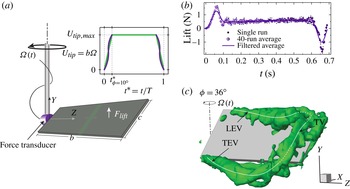
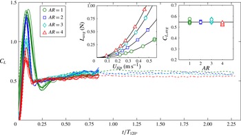
The experimental methods and previous results are depicted in figure 1 and summarized here, including lift force measurements and the prior S-DPIV of Carr et al. (Reference Carr, Chen and Ringuette2013a
). The experiments are conducted in a
 $91~\text{cm}\times 77~\text{cm}\times 71~\text{cm}$
glass tank containing a 50 % by mass glycerin–water mixture with a kinematic viscosity of
 $5.11\times 10^{-6}~\text{m}^{2}~\text{s}^{-1}$
. However, for the newer
 $\AR =4$
S-DPIV data set with closely matching
 $\mathit{Re}_{\mathit{span}}$
, the kinematic viscosity is
 $5.70\times 10^{-6}~\text{m}^{2}~\text{s}^{-1}$
, due to the tank temperature being colder at 18.7 °C, compared with 21 °C for the prior
 $\AR =2$
S-DPIV set and the force measurement cases. Figure 1(a) shows the wing-aligned coordinate system; the S-DPIV data are acquired and processed in a lab-fixed frame. The wings are rigid, rectangular flat plates with chord
 $c$
and span
 $b$
, and a fixed 45° angle of attack, attached to the drive shaft via low-profile clamps; the submersible force transducer can be affixed at the wing base and rotates with the wing. The plate thickness-to-chord ratio is
 ${\sim}$
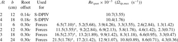
5 % or less, the edges are square, and the root offset (distance from the axis of rotation to the plate root) is given in table 1.
(a) The set-up, (b) force data and (c) a reconstructed flow volume.

Matrix of cases evaluated, with
 $\text{}^{\text{a}}$
indicating those where the final rotation angle
 ${\it\phi}_{\mathit{final}}=360^{\circ }$
is tested, in addition to the
 ${\it\phi}_{\mathit{final}}=120^{\circ }$
used for all cases.

The plates are driven from rest with a symmetric-in-time trapezoidal velocity using the tip velocity as a reference (figure 1
a inset, green line); for force measurements, hyperbolic tangents (purple lines) are used to smooth the accelerating portions of the motion program, to mitigate mechanical vibrations. The motion is a simplified hovering half-stroke, with parameters including
 $\AR =b^{2}/bc$
,
 $\mathit{Re}_{\mathit{span}}=U_{\mathit{tip}}b/{\it\nu}$
, where
 $U_{\mathit{tip}}$
is the maximum azimuthal plate tip velocity, rotation amplitude
 ${\it\phi}_{\mathit{final}}$
, and angle of attack consistent with large insects and hummingbirds (Dudley Reference Dudley1999; Tobalske et al.
Reference Tobalske, Warrick, Clark, Powers, Hedrick, Hyder and Biewener2007). The
 $\mathit{Re}_{\mathit{span}}$
for
 $\AR =2$
and 4 for S-DPIV are nearly matched at 10 700 and 10 433, respectively; the difference is 2.5 %. Acceleration from rest is over 10°; further parameters, including
 $\mathit{Re}_{\mathit{span}}$
for the force measurements,
 ${\it\phi}_{\mathit{final}}$
, and the maximum angular velocity, are provided in table 1.
The force transducer is an ATI Nano 17-IP68, sampled at 1 kHz; 40 runs are averaged for each case. The uncertainty from static tests is 0.63 % of the measurement for forces of
 $O$
(1) N. Raw force signals are low-pass filtered after averaging, with cutoffs chosen to eliminate noise and mechanical vibration. Figure 1(b) shows a single raw force measurement, the average of 40, and the filtered result for
 $\AR =2$
,
 $\mathit{Re}_{\mathit{span}}=11\,500$
.
Reconstructed S-DPIV volumes require data collection in multiple chordwise laser planes, achieved by translating the model along the span (
 $z$
-direction) with respect to the fixed S-DPIV system; the cameras are in a nearly symmetrical angular configuration. Figure 1(a) indicates the chordwise laser sheet orientation and spacing of consecutive planes. The volumetric data reconstructed from phase-locked, phase-averaged (
 $\times 5$
for
 $\AR =2$
, and
 $\times 7$
for the
 $\AR =4$
,
 $\mathit{Re}_{\mathit{span}}=10\,433$
case) S-DPIV have an angular resolution of 6°, an out-of-plane resolution of 0.06
 $c$
(0.08
 $c$
) for
 $\AR =2~(\AR=4)$
, with an in-plane resolution that is twice as fine. The uncertainty of the velocity measurement was examined thoroughly by Carr et al. (Reference Carr, Chen and Ringuette2013a
). The in-plane uncertainty, normalized by
 $U_{\mathit{tip}}$
, is
 ${\sim}$
0.01 corresponding to an approximately 0.1 pixel displacement for both
 $\AR\text{s}$
, and the uncertainty for the out-of-plane (
 $w$
) velocity is about twice this.
From the volumetric velocity data, three-dimensional vortex structures are identified using the
 ${\mathcal{Q}}$
-criterion (Hunt, Wray & Moin Reference Hunt, Wray and Moin1988); figure 1(c) indicates the LEV–TV–TEV loop. For the present paper, for volume renderings of
 ${\mathcal{Q}}$
isosurfaces only, a light
 $3\times 3$
Gaussian-weighted smoothing is done on the three-component velocity data in the S-DPIV (
 $x,y$
) planes prior to calculating the three-dimensional
 ${\mathcal{Q}}$
; this produces slightly clearer renderings. The methodology for computing spanwise circulation,
 ${\it\Gamma}$
, in chordwise (
 $x$
,
 $y$
), or constant-span, planes is described in § 3.1. Unless otherwise noted, quantities shown are normalized using
 $b$
and
 $U_{\mathit{tip}}$
, so that e.g. the vorticity is normalized by
 $U_{\mathit{tip}}/b$
.
3. Results and discussion
3.1. Spanwise circulation
Here we analyse the spatiotemporal variation of the spanwise leading-edge region vortex circulation, i.e. that in constant-span, or (
 $x$
,
 $y$
), planes using the S-DPIV data. We first examine different normalizations for comparing
 $\AR =2$
and 4, then focus on trends with
 $\AR$
. Two circulation quantities are used, the total circulation,
 ${\it\Gamma}_{\mathit{total}}$
, and that of the first LEV only,
 ${\it\Gamma}_{\mathit{LEV}}$
. The former is calculated as the area integral of the leading-edge region spanwise vorticity,
 ${\it\omega}_{z}$
, having the same sign as that of the LEV which is positive. It is a maximum reference value to which all (positive) spanwise leading-edge vortices contribute;
 ${\it\Gamma}_{\mathit{LEV}}$
is a subset of this.
3.1.1. Total circulation and vortex structure
To compute
 ${\it\Gamma}_{\mathit{total}}$
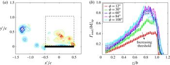
, the domain is restricted to a square region aligned with the plate chord and therefore the data grid (figure 2
a); for all
 ${\it\omega}_{z}$
fields presented, data below and ahead of the plate are not captured due to a laser shadow and the camera lines-of-sight being blocked by the plate. Measured from the plate suction side, the total circulation region is
 $1c$
above the plate for
 $\AR =2$
and
 $1.5c$
for
 $\AR =4$
, and extends the same distances, respectively, from the leading edge aft; the
 $\AR =4$
region is greater due to its larger outboard flow. These domains capture all of the positive
 ${\it\omega}_{z}$
in the leading-edge region flow, plus any
 ${\it\omega}_{z}>0$
near the plate, above the threshold described next, but exclude that sometimes residing in the trailing-edge flow which would incorrectly contribute to
 ${\it\Gamma}_{\mathit{total}}$
as defined here.
The
 ${\it\Gamma}_{\mathit{total}}$
processing methods. (a) Domain for calculating
 ${\it\Gamma}_{\mathit{total}}$
for
 $\AR =2$
, in plate-aligned (
 $x^{\prime }$
,
 $y^{\prime }$
) coordinates; data below and ahead of the plate are absent due to a laser shadow and line-of-sight blocking. (b) Effect of vorticity threshold,
 ${\it\omega}_{z,th}$
, on
 ${\it\Gamma}_{\mathit{total}}$
(
 $\AR =2$
); for each
 ${\it\phi}$
, the four curves indicate
 ${\it\omega}_{z,th}=0$
,
 $0.5\overline{{\it\omega}_{z}}$
,
 $1.0\overline{{\it\omega}_{z}}$
and
 $1.5\overline{{\it\omega}_{z}}$
, respectively.

A spanwise vorticity threshold,
 ${\it\omega}_{z,th}$
, is incorporated to remove any background vorticity below the uncertainly level. It is employed in obtaining both
 ${\it\Gamma}_{\mathit{total}}$
and
 ${\it\Gamma}_{\mathit{LEV}}$
. For use only to examine the sensitivity of the circulation to this threshold, similar to DeVoria & Ringuette (Reference DeVoria and Ringuette2012) a (normalized) reference vorticity value is chosen as the spatial and temporal mean of the positive
 ${\it\omega}_{z}$
residing within the square regions just described, referred to as
 $\overline{{\it\omega}_{z}}$
, using all rotation angles
 ${\it\phi}$
and all spanwise data planes (
 $z$
positions). The values of
 $\overline{{\it\omega}_{z}}$
, normalized using
 $b$
, are 2.76 and 3.84 for
 $\AR =2$
and 4. Carr et al. (Reference Carr, Chen and Ringuette2013a
) showed that the maximum uncertainty in the non-dimensional vorticity for these data sets is
 ${\sim}$
0.04 using
 $c$
for normalization, which becomes 0.08 and 0.16 for
 $\AR =2$
and 4, respectively, when normalizing via
 $b$
; thus,
 $\overline{{\it\omega}_{z}}$
is much larger than the uncertainty.
To illustrate the effect of varying
 ${\it\omega}_{z,th}$
, figure 2(b) shows
 ${\it\Gamma}_{\mathit{total}}^{\ddagger }={\it\Gamma}_{\mathit{total}}/bU_{\mathit{tip}}$
(as discussed below) plotted against the normalized spanwise position,
 $z/b$
, for
 $\AR =2$
. The coloured curves indicate different values of
 ${\it\phi}$
, and for each
 ${\it\phi}$
four curves are shown, ranging from
 ${\it\omega}_{z,th}=0$
to
 $1.5\overline{{\it\omega}_{z}}$
in increments of
 $0.5\overline{{\it\omega}_{z}}$
. The highest values of
 ${\it\Gamma}_{\mathit{total}}^{\ddagger }$
correspond to
 ${\it\omega}_{z,th}=0$
, and
 ${\it\Gamma}_{\mathit{total}}^{\ddagger }$
decreases only slightly with each relatively large increase in
 ${\it\omega}_{z,th}$
. For the entire
 ${\it\omega}_{z,th}=0{-}1.5\overline{{\it\omega}_{z}}$
range, there is a
 ${\sim}$
20 % decrease in
 ${\it\Gamma}_{\mathit{total}}^{\ddagger }$
near 20 % span, where the circulation values are small, which reduces to
 ${\sim}$
10 % in the peak regions near the tip. The value of
 ${\it\omega}_{z,th}$
has a negligible effect on the observed trends, and
 ${\it\Gamma}_{\mathit{total}}^{\ddagger }$
is relatively insensitive to it since from
 ${\it\omega}_{z,th}=0$
to
 $0.5\overline{{\it\omega}_{z}}$
the
 ${\it\Gamma}_{\mathit{total}}^{\ddagger }$
decreases only
 ${\sim}$
7 % for 20 % span and
 ${\sim}$
2 % in the tip region. A matching numerical value of
 ${\it\omega}_{z,th}=0.2$
is chosen for each
 $\AR$
, which is slightly above the span-normalized uncertainties reported earlier.
We first explore various normalizations of the circulation to better isolate
 $\AR$
effects, including those which produce the best agreement in the spatial and temporal trends. Figure 3 shows normalized curves of
 ${\it\Gamma}_{\mathit{total}}$
versus
 $z/b$
; plotting the
 ${\it\Gamma}_{\mathit{total}}$
versus
 $z/c$
for
 $\AR =2$
and 4 shows poorer agreement in all cases. For each plot in figure 3, multiple curves are shown which indicate the circulation at different times. One method for comparing the flow evolution with time for each
 $\AR$
is to match the chord lengths travelled by the tip,
 $(s/c)_{\mathit{tip}}$
, which also matches the chords traversed at a given
 $z/b$
. Note that, neglecting the small wing root offset,
 $(s/c)_{\mathit{tip}}=\AR {\it\phi}$
. Therefore, when matching
 $(s/c)_{\mathit{tip}}$
for each
 $\AR$
, the value of
 ${\it\phi}$
for
 $\AR =4$
is half that for
 $\AR =2$
.
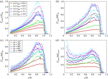
Plots of
 ${\it\Gamma}_{\mathit{total}}$
using various normalizations, versus normalized spanwise location
 $z/b$
: (a)
 ${\it\Gamma}_{\mathit{total}}/cU_{\mathit{tip}}$
for matching
 $(s/c)_{\mathit{tip}}$
; (b)
 ${\it\Gamma}_{\mathit{total}}/bU_{\mathit{tip}}$
for matching
 $(s/c)_{\mathit{tip}}$
; (c)
 ${\it\Gamma}_{\mathit{total}}/bU_{\mathit{tip}}$
for matching
 ${\it\phi}$
; (d)
 ${\it\Gamma}_{\mathit{total}}/bU_{\mathit{local}}$
for matching
 ${\it\phi}$
. Solid lines:
 $\AR =2$
; dashed:
 $\AR =4$
. The legend for (a) applies to (b), the legend for (c) applies to (d).

Normalizing circulation first by the chord length and reference velocity,
 $U_{\mathit{tip}}$
, gives
 ${\it\Gamma}_{\mathit{total}}^{\dagger }={\it\Gamma}_{\mathit{total}}/(cU_{\mathit{tip}})$
. Figure 3(a) shows
 ${\it\Gamma}_{\mathit{total}}^{\dagger }$
versus
 $z/b$
, with curves for
 $(s/c)_{\mathit{tip}}=0.4{-}4.0$
. For
 $(s/c)_{\mathit{tip}}=0.4$
, the
 $\AR =2$
circulation is larger. This may be due to the fact that the rotational acceleration is accomplished over matching
 ${\it\phi}=10^{\circ }$
and not
 $(s/c)_{\mathit{tip}}$
. At
 $(s/c)_{\mathit{tip}}=0.4$
the
 $\AR =2$
plate has travelled
 ${\it\phi}=12^{\circ }$
and acceleration is completed, whereas the
 $\AR =4$
plate is at
 ${\it\phi}=6^{\circ }$
and still accelerating. After the startup, for
 $(s/c)_{\mathit{tip}}=0.9$
and 2.2 the curves of
 ${\it\Gamma}_{\mathit{total}}^{\dagger }$
for
 $\AR =2$
and 4 show reasonably good agreement. However, as
 $(s/c)_{\mathit{tip}}$
increases further, the differences between the
 ${\it\Gamma}_{\mathit{total}}^{\dagger }$
become substantial outboard of
 $z/b\approx 0.4$
.
Next, following Harbig et al. (Reference Harbig, Sheridan and Thompson2013) the circulation is normalized by the plate span, giving
 ${\it\Gamma}_{\mathit{total}}^{\ddagger }={\it\Gamma}_{\mathit{total}}/(bU_{\mathit{tip}})$
; alternatively, this can be written as
 ${\it\Gamma}_{\mathit{total}}^{\ddagger }={\it\Gamma}_{\mathit{total}}^{\dagger }/\AR$
. Figure 3(b) plots
 ${\it\Gamma}_{\mathit{total}}^{\ddagger }$
versus
 $(s/c)_{\mathit{tip}}$
. With this normalization, the circulation curves for each
 $\AR$
are in comparatively worse agreement for all
 $(s/c)_{\mathit{tip}}$
, with the
 $\AR =2$
circulation being consistently higher, versus employing
 ${\it\Gamma}_{\mathit{total}}^{\dagger }$
. Another option is to compare the different
 $\AR$
data at matching
 ${\it\phi}$
, analogous to matching
 $(s/b)_{\mathit{tip}}$
, which Carr et al. (Reference Carr, Chen and Ringuette2013a
) indicated to be best for comparison of the vortex structures for the overall
 ${\it\phi}=120^{\circ }$
motion. In figure 3(c),
 ${\it\Gamma}_{\mathit{total}}^{\ddagger }$
is plotted with colored curves signifying matching
 ${\it\phi}$
for
 $\AR =2$
and 4; the
 ${\it\phi}$
range is 12–108°. Note that the green curve for
 $\AR =2$
is for
 ${\it\phi}=24^{\circ }$
in figure 3(a) and
 ${\it\phi}=30^{\circ }$
in figure 3(c). By matching
 ${\it\phi}$
, the
 $\AR =2$
and 4 curves of
 ${\it\Gamma}_{\mathit{total}}^{\ddagger }$
are much closer in magnitude for higher rotation angles,
 ${\it\phi}\geqslant 60^{\circ }$
, compared to matching
 $(s/c)_{\mathit{tip}}$
for
 ${\it\Gamma}_{\mathit{total}}^{\dagger }$
or
 ${\it\Gamma}_{\mathit{total}}^{\ddagger }$
.
Overall, the
 $\AR$
differences are somewhat lessened if
 $b$
is used as the length scale in normalizing
 ${\it\Gamma}_{\mathit{total}}$
, consistent with Harbig et al. (Reference Harbig, Sheridan and Thompson2013), and if the results are compared at matching
 ${\it\phi}$
(or
 $(s/b)_{\mathit{tip}}$
), particularly for larger
 ${\it\phi}$
. However, although these normalizations may reduce
 $\AR$
variations and therefore provide an appropriate framework for comparisons, there remain some significant differences with
 $\AR$
as discussed below.
The total circulation behaviour is described here. Figure 3(c) shows that for all values of
 ${\it\phi}$
and both
 $\AR\text{s}$
, there is a general increase in
 ${\it\Gamma}_{\mathit{total}}^{\ddagger }$
with span after
 ${\sim}$
20 % span, followed by a maximum within
 $0.7<z/b<1$
. A sharp drop to zero is found past the tip where reorientation of some of the LEV spanwise vorticity to streamwise vorticity,
 ${\it\omega}_{x}$
, occurs during aft tilt and lift-off (described later), and also
 ${\it\omega}_{x}$
from the TV is dominant.
Figure 3(c) also shows a clear variation with
 $\AR$
, namely the
 $\AR =2$
 ${\it\Gamma}_{\mathit{total}}^{\ddagger }$
is higher for nearly all data points across the span for each
 ${\it\phi}$
; again, this difference is relatively larger for lower
 ${\it\phi}$
. Harbig et al. (Reference Harbig, Sheridan and Thompson2013) calculated the sum of the circulations of the dual-LEVs they found (§ 1), analogous to the present total circulation, for their
 $\mathit{Re}_{\mathit{span}}=3833$
case at
 ${\it\phi}=270^{\circ }$
and for
 $\AR =2.91{-}7.28$
Drosophila planforms. They normalized it using
 $b$
and the velocity at the radius of gyration, and showed a decrease in circulation with increasing
 $\AR$
across the span; therefore the current results are consistent with these simulations. Further, the present data show a weakening dependence of
 ${\it\Gamma}_{\mathit{total}}^{\ddagger }$
on
 ${\it\phi}$
with larger values for
 ${\it\phi}>30^{\circ }$
, for both
 $\AR\text{s}$
. In the tip region, the differences between
 ${\it\Gamma}_{\mathit{total}}^{\ddagger }$
for
 $\AR =2$
and 4 are relatively larger, particularly for
 ${\it\phi}=108^{\circ }$
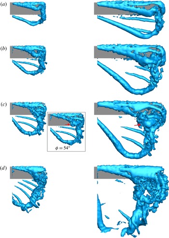
. This can be explained by examining the three-dimensional flow structure shown by an isosurface of
 ${\mathcal{Q}}$
, which is provided in figure 4 for
 $\AR =2$
and 4 from
 ${\it\phi}=30^{\circ }$
to 90°.
Top, or (
 $x$
,
 $z$
)-plane, view of an iso-surface of non-dimensional
 ${\mathcal{Q}}=12$
at (a)
 ${\it\phi}=30^{\circ }$
, (b)
 ${\it\phi}=48^{\circ }$
, (c)
 ${\it\phi}=60^{\circ }$
and (d)
 ${\it\phi}=90^{\circ }$
;
 $\AR =2$
(left column) and 4 (right column). The red arrow indicates LEV enlargement prior to breakdown.

Considering
 ${\it\phi}=30^{\circ }$
, the isosurfaces show some similarities between the
 $\AR =2$
and 4 flow structures, including outboard LEV lift-off into an arch-like structure, and a ‘stable’ LEV inboard; the latter persists for all
 ${\it\phi}$
. These features are in good agreement with the
 $\AR =2$
and 4 simulations of Garmann & Visbal (Reference Garmann and Visbal2014), the
 $\AR =4$
computation of Jardin et al. (Reference Jardin, Farcy and David2012) and the
 $\AR =1{-}3$
volumetric data of Ozen & Rockwell (Reference Ozen and Rockwell2012, Reference Ozen and Rockwell2013). As the first LEV lifts off, another forms ahead of it which connects to the TV for both
 $\AR\text{s}$
(
 ${\it\phi}=30^{\circ }$
). It is the contributions from these further, outboard LEVs for both
 $\AR\text{s}$
which cause the larger increase in
 ${\it\Gamma}_{\mathit{total}}^{\ddagger }$
for
 $0.6<z/b<0.8$
and
 ${\it\phi}\geqslant 30^{\circ }$
(figure 3
c), although breakdown then acts to reduce the
 $\AR =4$
outboard circulation as described below.
Despite the flow similarities just mentioned, there is a substantial
 $\AR$
variation at
 ${\it\phi}=30^{\circ }$
. Namely, at a given
 $z/b$
the
 $\AR =4$
LEV structures are located farther aft from the leading edge than for the shorter-span
 $\AR =2$
plate. For example, a part of the
 $\AR =4$
lifted-off LEV has already moved past the trailing-edge location; also, the lifted-off LEV for
 $\AR =4$
appears larger. The
 $\AR =4$
aft LEV tilt at
 ${\it\phi}=30^{\circ }$
is thus more substantial at a given
 $z/b$
than for
 $\AR =2$
, as quantified in figure 9 (solid magenta line). As discussed in § 3.1.3, this leads to a reduction in spanwise circulation, and is likely the main reason for the smaller
 ${\it\Gamma}_{\mathit{total}}^{\ddagger }$
for
 $\AR =4$
. In addition, the iso-
 ${\mathcal{Q}}$
surface at
 ${\it\phi}=30^{\circ }$
shows that the portion of the TV aft of the trailing edge for
 $\AR =4$
is positioned more inboard than the TV structure residing over the tip edge itself; for
 $\AR =2$
, these two TV segments are well-aligned, although similar behaviour occurs at higher
 ${\it\phi}$
.
As
 ${\it\phi}$
increases, flow structure variations with
 $\AR$
persist. For
 $\AR =4$
, the second outboard LEV lifts off to form an arch which connects to the TV (
 ${\it\phi}=48^{\circ }$
), and a further LEV forms ahead of this. By
 ${\it\phi}=60^{\circ }$
, the outboard
 $\AR =4$
flow shows three smaller LEVs ahead of the initial one, which has by this time moved aft of the trailing edge. Concurrently, the initial, main TV also travels off the plate and exists primarily behind the trailing edge; in addition, a smaller streamwise (tip-oriented) structure is visible just outside of the tip edge as well as aft of the outboard plate corner, connected to the smaller LEVs. For
 $\AR =4$
the outboard LEV becomes larger (
 ${\it\phi}=60^{\circ }$
, red arrow), which is a sign of breakdown (Delery Reference Delery1994; Lucca-Negro & O’Doherty Reference Lucca-Negro and O’Doherty2001) and a similar LEV size increase was found by Lu & Shen (Reference Lu and Shen2008) and Garmann & Visbal (Reference Garmann and Visbal2014); also smaller vortical structures are visible around it. By
 ${\it\phi}=90^{\circ }$
, for
 $\AR =4$
the outboard breakdown has progressed substantially, qualitatively indicated by small, unorganized structures. This breakdown is responsible for the reduction in outboard
 ${\it\Gamma}_{\mathit{total}}^{\ddagger }$
from
 ${\it\phi}=84^{\circ }$
to 108° (figure 3
c). The breakdown adversely affects the mean-flow convergence from phase averaging (Carr et al.
Reference Carr, Chen and Ringuette2013a
), leading to the reduced coherence observed in the iso-
 ${\mathcal{Q}}$
surfaces and the outboard, high-
 ${\it\phi}$
vorticity fields (figures 7 and 8).
Conversely, for
 $\AR =2$
the initial, outboard LEV does not move past the trailing edge after lift-off, but by
 ${\it\phi}=60^{\circ }$
it has tilted aft and merged with the TV, and both are close to the plate. An inset giving the flow at
 ${\it\phi}=54^{\circ }$
shows an increase in the size of this aft-tilted LEV (red arrow), which as for
 $\AR =4$
indicates a breakdown event; this flow structure becomes more complex at
 ${\it\phi}=60^{\circ }$
. By
 ${\it\phi}=90^{\circ }$
, the outboard
 $\AR =2$
LEV/TV flow shows prominent breakdown with a leading-edge shear layer ahead of it that is deflected away from the plate; the
 $\AR =4$
case exhibits a similar leading-edge shear layer (see also figures 7 and 8, 70 % span). The present breakdown behaviour is similar in terms of spatial location and timing to that of the
 $\AR =2$
and 4 rotating-wing dye flow visualizations of Carr & Ringuette (Reference Carr and Ringuette2014). Despite the breakdown, the
 $\AR =2$
outboard flow remains more coherent and resides over plate, compared with
 $\AR =4$
, yielding the higher
 ${\it\Gamma}_{\mathit{total}}^{\ddagger }$
.
A local minimum for
 ${\it\Gamma}_{\mathit{total}}^{\ddagger }$
is found near or just outboard of 90 % span for
 $30^{\circ }\leqslant {\it\phi}\leqslant 60^{\circ }$
for
 $\AR =2$
and 4 (e.g. figure 3
c, black arrow); at higher
 ${\it\phi}$
the
 ${\it\Gamma}_{\mathit{total}}^{\ddagger }$
reduction for
 $\AR =4$
is from breakdown. The iso-
 ${\mathcal{Q}}$
surfaces show that this coincides with the outboard ‘foot’ of the lifted-off, arch-like LEV (figure 4). This ‘foot’ tilts upward so some of its originally spanwise vorticity is converted into
 $x$
- and
 $y$
-direction vorticity, causing lower
 ${\it\Gamma}_{\mathit{total}}^{\ddagger }$
. This also results in the
 ${\it\Gamma}_{\mathit{total}}^{\ddagger }$
maximum moving somewhat inboard with higher
 ${\it\phi}$
.
Given the increase of
 ${\it\Gamma}_{\mathit{total}}^{\ddagger }$
with
 $z/b$
away from the tip, using instead the maximum plate azimuthal velocity at each (local) spanwise position,
 $U_{\mathit{local}}$
, to normalize it yields more comparable values across the span (figure 3
d); we define it as
 ${\it\Gamma}_{\mathit{total}}^{\ast }={\it\Gamma}_{\mathit{total}}/(bU_{\mathit{local}})$
. Circulation normalization using
 $U_{\mathit{local}}$
was also employed by Carr, DeVoria & Ringuette (Reference Carr, DeVoria and Ringuette2013b
) and Wojcik & Buchholz (Reference Wojcik and Buchholz2014a
). For
 ${\it\phi}=12^{\circ }$
, when the influence of the plate ends is small, the curves of
 ${\it\Gamma}_{\mathit{total}}^{\ast }$
are nearly flat between the root and tip. This indicates that the strength of the LEV scales proportionally to the local plate velocity. For higher
 ${\it\phi}$
,
 ${\it\Gamma}_{\mathit{total}}^{\ast }$
grows relatively larger toward the root and outboard of
 $z/b\approx 0.6$
except very near the tip, and the
 $U_{\mathit{local}}$
normalization is insufficient to remove spanwise variations in these regions. Outboard, this is due to the highly three-dimensional flow structure, including LEV lift-off, shown earlier. The values of
 ${\it\Gamma}_{\mathit{total}}^{\ast }$
near the root are somewhat amplified because of the division by very small
 $U_{\mathit{local}}$
. Between 20 % and 60 % span the variations in
 ${\it\Gamma}_{\mathit{total}}^{\ast }$
are significantly reduced, compared with using
 $U_{\mathit{tip}}$
. The 20–60 % spanwise range overlaps the locations where Carr et al. (Reference Carr, Chen and Ringuette2013a
) identified the LEV to be ‘stable’, i.e. for up to
 ${\sim}$
40–50 % span for
 $\AR =4$
and up to
 ${\sim}$
60 % for
 $\AR =2$
(also shown here in figure 4). Therefore, in the ‘stable’ LEV the circulation scales with the local azimuthal velocity; this holds even at the highest
 ${\it\phi}$
acquired prior to deceleration, 108°. Although this normalization is less successful near the plate ends, it remains useful for examining temporal trends and producing spanwise averages.
As shown above, the overall evolution of
 ${\it\Gamma}_{\mathit{total}}$
with time is most similar for
 $\AR =2$
and 4 at matching
 ${\it\phi}$
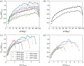
. Figure 5(a) plots
 ${\it\Gamma}_{\mathit{total}}^{\ast }$
against
 ${\it\phi}$
with multiple curves from 20 % to 80 % span in 10 % increments for
 $\AR =2$
and 4. For each
 $\AR$
the circulation has a higher initial slope, then beyond
 ${\it\phi}\approx 42^{\circ }$
the slope gradually reduces but remains generally positive, albeit with some fluctuations and differences at each spanwise position. Reflecting the results of figure 3(d), for each
 $\AR$
the individual-span curves have similar magnitudes for inboard locations, but increase in magnitude for 60–80 % span toward the tip region.
Plots of
 ${\it\Gamma}_{\mathit{total}}$
versus
 ${\it\phi}$
or chords travelled: (a)
 ${\it\Gamma}_{\mathit{total}}/bU_{\mathit{local}}$
versus
 ${\it\phi}$
at different spanwise locations; (b) spanwise-averaged
 ${\it\Gamma}_{\mathit{total}}/bU_{\mathit{local}}$
over 20–80 % span versus
 ${\it\phi}$
; (c)
 ${\it\Gamma}_{\mathit{total}}/bU_{\mathit{local}}$
versus
 $(s/c)_{\mathit{local}}$
for
 $\AR =2$
; (d) same, but for
 $\AR =4$
. Solid lines:
 $\AR =2$
; dashed:
 $\AR =4$
.

Figure 5(b) shows the spanwise average of
 ${\it\Gamma}_{\mathit{total}}^{\ast }$
from 20 % to 80 % span, away from the plate ends, which yields clearer trends. The
 $\AR =2$
magnitudes are again larger, but what is most striking is the similarity in the slopes of the curves after
 ${\it\phi}=24^{\circ }$
, until deceleration. This feature is discussed again in the context of the lift coefficient in § 3.4.
We also examine the evolution of
 ${\it\Gamma}_{\mathit{total}}^{\ast }$
with local chord lengths travelled,
 $(s/c)_{\mathit{local}}$
, at each
 $z/b$
(figure 5
c,d for
 $\AR =2$
and 4, respectively); this was also done by Poelma et al. (Reference Poelma, Dickson and Dickinson2006) for the LEV. At a given
 $z/b$
, the
 $\AR =2$
plate travels approximately half the distance covered by
 $\AR =4$
for matching
 ${\it\phi}$
. For
 $\AR =2$
, up to
 $(s/c)_{\mathit{local}}\approx 1$
the
 ${\it\Gamma}_{\mathit{total}}^{\ast }$
curves from 30 % to 80 % span collapse reasonably well, then the slope of each decreases. The individual-span curves then diverge at slightly different values of
 $(s/c)_{\mathit{local}}$
. The initial collapse of the
 ${\it\Gamma}_{\mathit{total}}^{\ast }$
curves indicates a growth based on
 $(s/c)_{\mathit{local}}$
. This explains why matching
 ${\it\phi}$
is not as successful in characterizing temporal trends with
 $\AR$
for smaller
 ${\it\phi}$
. After
 $(s/c)_{\mathit{tip}}\approx 1$
, events such as outboard LEV lift-off and more complex tip-region flow occur which change the growth rate. Apart from the 20 % span values, the initial collapse of the
 $\AR =4$
curves occurs over a larger
 $(s/c)_{\mathit{local}}\approx 2$
, indicating a longer distance travelled for features such as plate end effects to manifest, which makes sense due to the higher
 $\AR$
. Following this, the individual curves diverge similar to
 $\AR =2$
. This initial
 ${\it\Gamma}_{\mathit{total}}$
collapse is consistent with that of the LEV circulation shown by Poelma et al. (Reference Poelma, Dickson and Dickinson2006) for a single
 $\AR$
. Jardin et al. (Reference Jardin, Farcy and David2012) found a linear increase in non-dimensional LEV circulation with non-dimensional distance travelled for
 $\AR =4$
at a given spanwise location, but that the coefficient varied with span; here we do not find a linear increase overall, however, it is characterized by chords travelled up to
 $(s/c)_{\mathit{local}}\approx 2$
.
3.1.2. LEV circulation and flow fields
To obtain
 ${\it\Gamma}_{\mathit{LEV}}$
, following DeVoria & Ringuette (Reference DeVoria and Ringuette2012) the centre of the first LEV formed is identified and tracked using the maximum positive
 ${\it\omega}_{z}$
. The search for subsequent LEV centres is restricted to a window (
 $9\times 9$
grid points for
 $\AR =2$
,
 $7\times 7$
for
 $\AR =4$
) surrounding the previous
 ${\it\omega}_{z}$
maximum, which aids in avoiding other vortices or any stronger
 ${\it\omega}_{z}$
in the leading-edge shear layer; this plants a ‘seed’ point in the first LEV at each time step. Starting with this point, a clustering algorithm connects adjacent points which make up the LEV, if the in-plane
 ${\mathcal{Q}}$
, i.e.
 ${\mathcal{Q}}_{2D}$
, is greater than 0; this indicates a local rotation rate greater than the strain rate (Chakraborty, Balachandar & Adrian Reference Chakraborty, Balachandar and Adrian2005). The three-dimensional
 ${\mathcal{Q}}$
is not used since it is influenced by out-of-plane flow, and a threshold of 0 is chosen to obtain the maximum possible identified vortex points. The actual LEV centre location is then determined from the
 ${\it\omega}_{z}$
-weighted centroid of each cluster, after the following procedure is performed.
The
 ${\mathcal{Q}}_{2D}$
is often too restrictive and does not identify data in the outer portion of the LEV having comparable
 ${\it\omega}_{z}$
, which yields lower
 ${\it\Gamma}_{\mathit{LEV}}$
. We correct for this, as done by DeVoria & Ringuette (Reference DeVoria and Ringuette2012), by searching for any further grid points having
 ${\it\omega}_{z}>{\it\omega}_{z,th}$
that are no greater than
 $2\sqrt{2}$
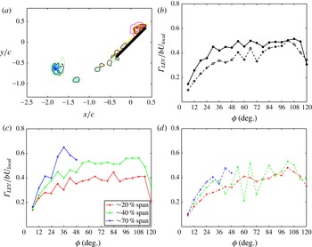
grid spacings from at least one point in the original cluster, and then appending them into the (augmented) set. Figure 6(a) shows a
 ${\it\omega}_{z}$
field for
 $\AR =2$
with a black contour indicating the originally identified cluster and a magenta contour showing the augmented cluster. Similar to
 ${\it\Gamma}_{\mathit{total}}$
, the
 ${\it\Gamma}_{\mathit{LEV}}^{\ast }$
exhibits insensitivity to the
 ${\mathcal{Q}}_{2D}$
threshold used, in part due to the cluster augmentation, with reductions of typically less than 6 % when comparing results using
 ${\mathcal{Q}}_{2D}>0$
versus (non-dimensional)
 ${\mathcal{Q}}_{2D}>5$
.
LEV circulation: (a) LEV identified using
 ${\mathcal{Q}}_{2D}>0$
only (black contour) and additional clustering (magenta contour); (b) spanwise-averaged
 ${\it\Gamma}_{\mathit{LEV}}^{\ast }$
over ‘stable’ LEV (20–60 % span for
 $\AR =2$
, 20–40 % span for
 $\AR =4$
); (c)
 ${\it\Gamma}_{\mathit{LEV}}^{\ast }$
versus
 ${\it\phi}$
,
 $\AR =2$
; (d)
 ${\it\Gamma}_{\mathit{LEV}}^{\ast }$
versus
 ${\it\phi}$
,
 $\AR =4$
; solid lines:
 $\AR =2$
; dashed:
 $\AR =4$
.

To examine the temporal trends of
 ${\it\Gamma}_{\mathit{LEV}}$
and compare
 $\AR =2$
and 4, we plot
 ${\it\Gamma}_{\mathit{LEV}}^{\ast }$
versus
 ${\it\phi}$
(figure 6). Figure 6(b) gives black lines showing the spanwise average of
 ${\it\Gamma}_{\mathit{LEV}}^{\ast }$
across the perpetually ‘stable’ LEV, from 20–60 % span and 20–40 % span for
 $\AR =2$
and 4, respectively. Reflecting the behaviour of
 ${\it\Gamma}_{\mathit{total}}^{\ast }$
, the span-averaged
 ${\it\Gamma}_{\mathit{LEV}}^{\ast }$
for
 $\AR =2$
is generally larger. For each
 $\AR$
, these mean curves have their highest growth rates for
 ${\it\phi}=24{-}36^{\circ }$
, after which the
 $\AR =2$
circulation essentially levels off or saturates (apart from some fluctuations) while that for
 $\AR =4$
increases at a slow rate and peaks before deceleration; fluctuations in the
 $\AR =4$
span-averaged curve are due to values at 40 % span as explained below. The initial greater increase of
 ${\it\Gamma}_{\mathit{LEV}}$
followed by a leveling off or slower growth is consistent with the rotating
 $\AR =2.3$
plate results of Kim & Gharib (Reference Kim and Gharib2010) for trapezoidal velocity programs. Poelma et al. (Reference Poelma, Dickson and Dickinson2006) also showed
 ${\it\Gamma}_{\mathit{LEV}}$
levelling off, or slightly increasing or decreasing, depending on the spanwise location.
Figure 6(c,d) show curves of
 ${\it\Gamma}_{\mathit{LEV}}^{\ast }$
at 20 % and 40 % span, within the ‘stable’ LEV, and outboard at 70 % span, for
 $\AR =2$
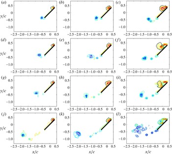
and 4, respectively. In figures 7 and 8, corresponding
 ${\it\omega}_{z}$
fields are shown for
 ${\it\phi}=30^{\circ }{-}90^{\circ }$
. In these figures, the solid black contour outlines the identified LEV, but in some instances a value of
 ${\mathcal{Q}}_{2D}=0.1$
is given (dash-dot black line) to indicate problems with identification of the first LEV caused by breakdown.
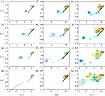
Spanwise vorticity fields at specified spanwise positions and
 ${\it\phi}$
,
 $\AR =2$
. Contour lines range from
 $-44$
to
 $-4$
and 4 to 44 in steps of 5. Solid black line, identified LEV; dashed black line,
 ${\mathcal{Q}}_{2D}=0.1$
: (a) 20 % span,
 ${\it\phi}=30^{\circ }$
; (b) 40 % span,
 ${\it\phi}=30^{\circ }$
; (c) 70 % span,
 ${\it\phi}=30^{\circ }$
; (d) 20 % span,
 ${\it\phi}=48^{\circ }$
; (e) 40 % span,
 ${\it\phi}=48^{\circ }$
; (f) 70 % span,
 ${\it\phi}=48^{\circ }$
; (g) 20 % span,
 ${\it\phi}=60^{\circ }$
; (h) 40 % span,
 ${\it\phi}=60^{\circ }$
; (i) 70 % span,
 ${\it\phi}=60^{\circ }$
; (j) 20 % span,
 ${\it\phi}=90^{\circ }$
; (k) 40 % span,
 ${\it\phi}=90^{\circ }$
; (l) 70 % span,
 ${\it\phi}=90^{\circ }$
.

Spanwise vorticity fields at specified spanwise positions and
 ${\it\phi}$
,
 $\AR =4$
. Same contour levels as figure 7: (a) 20 % span,
 ${\it\phi}=30^{\circ }$
; (b) 40 % span,
 ${\it\phi}=30^{\circ }$
; (c) 70 % span,
 ${\it\phi}=30^{\circ }$
; (d) 20 % span,
 ${\it\phi}=48^{\circ }$
; (e) 40 % span,
 ${\it\phi}=48^{\circ }$
; (f) 70 % span,
 ${\it\phi}=48^{\circ }$
; (g) 20 % span,
 ${\it\phi}=60^{\circ }$
; (h) 40 % span,
 ${\it\phi}=60^{\circ }$
; (i) 70 % span,
 ${\it\phi}=60^{\circ }$
; (j) 20 % span,
 ${\it\phi}=90^{\circ }$
; (k) 40 % span,
 ${\it\phi}=90^{\circ }$
; (l) 70 % span,
 ${\it\phi}=90^{\circ }$
.

At 20 % span the
 ${\it\Gamma}_{\mathit{LEV}}^{\ast }$
curves for each
 $\AR$
reflect the temporal trends of the span average, although the magnitudes for
 $\AR =2$
and 4 are more comparable. Inspection of the
 ${\it\omega}_{z}$
fields indicates that the LEV remains closely attached to the plate at 20 % span, and that there are small changes in the LEV vorticity distribution and its identification with time that lead to the fluctuations in
 ${\it\Gamma}_{\mathit{LEV}}^{\ast }$
for both
 $\AR$
.
For
 $\AR =2$
,
 ${\it\Gamma}_{\mathit{LEV}}^{\ast }$
at 40 % span is higher than at 20 %, but with a similar time evolution. Correspondingly, the LEV is larger, it does not evolve substantially although its size fluctuates, and it remains close to the plate (figure 7). However, the
 $\AR =4$
case shows substantial variations between
 ${\it\phi}=36^{\circ }$
and 90°. The vorticity fields in figure 8 reveal the cause, namely after
 ${\it\phi}=30^{\circ }$
the leading-edge vorticity is typically organized in one of two ways: (i) one large LEV as well as further positive
 ${\it\omega}_{z}$
ahead of this, which is the LEV shear layer (
 ${\it\phi}=48^{\circ }$
); (ii) two LEVs of either approximately equal size (
 ${\it\phi}=60^{\circ }$
) or with a larger initial one and smaller second one ahead of it (
 ${\it\phi}=42^{\circ }$
and 72°, not shown), both smaller than the single LEV of case (i); the tracking algorithm identifies the first LEV formed. The
 ${\it\Gamma}_{\mathit{LEV}}^{\ast }$
is therefore larger for case (i) and yields a local minimum for case (ii) (figure 6
d). The iso-
 ${\mathcal{Q}}$
surfaces (figure 4) indicate a ‘split’ of the
 $\AR =4$
LEV around 40 % span, whose spanwise position fluctuates, as previously shown by Carr et al. (Reference Carr, Chen and Ringuette2013a
). For
 $\AR =2$
, inspection of the
 ${\it\omega}_{z}$
fields and iso-
 ${\mathcal{Q}}$
surfaces indicates an LEV ‘split’ location of
 ${\sim}$
60 % span. As mentioned above, Harbig et al. (Reference Harbig, Sheridan and Thompson2013) also showed ‘split’ LEVs for all
 $\AR\text{s}$
tested for
 $Re_{\mathit{span}}\approx 1000$
and higher. However, unlike Harbig et al. (Reference Harbig, Sheridan and Thompson2013) the present ‘split’ locations are not the same for both
 $\AR\text{s}$
despite the matching
 $\mathit{Re}_{\mathit{span}}$
. This may be a function of the slightly higher
 $\mathit{Re}_{\mathit{span}}$
here, the wing geometry (rectangular versus fruit fly), or the S-DPIV resolution.
The
 ${\it\Gamma}_{\mathit{LEV}}^{\ast }$
at 70 % span is larger for
 $\AR =2$
compared with 4, consistent with the outboard trends of
 ${\it\Gamma}_{\mathit{total}}^{\ast }$
. For
 $\AR =2$
,
 ${\it\Gamma}_{\mathit{LEV}}^{\ast }$
for 70 % span peaks at
 ${\it\phi}=36^{\circ }$
then decreases, while for
 $\AR =4$
it peaks at
 ${\it\phi}=42^{\circ }$
. The curves at 70 % span for each
 $\AR$
do not extend over the full
 ${\it\phi}$
range, because after they stop the first LEV can no longer be clearly identified using
 ${\mathcal{Q}}_{2D}$
. This is illustrated by plotting dash-dot black contours of
 ${\mathcal{Q}}_{2D}=0.1$
for
 $\AR =2$
at
 ${\it\phi}=90^{\circ }$
(figure 7
l) and for
 $\AR =4$
at
 ${\it\phi}=60^{\circ }$
, 90° (figure 8
i,l). There are multiple and more complex vortex structures than at earlier
 ${\it\phi}$
(and compared with smaller spanwise locations), and the identification and tracking algorithm becomes unreliable. This is due to factors such as LEV breakdown, and an LEV–TV interaction for
 $\AR =2$
(figure 4).
The
 $\AR =2~{\it\omega}_{z}$
fields in figure 7 at 20 % span additionally show that the TEV (largest region of
 ${\it\omega}_{z}<0$
) travels aft with
 ${\it\phi}$
as expected. Discrete vortices having
 ${\it\omega}_{z}<0$
are visible in the separated trailing-edge flow at
 ${\it\phi}=60^{\circ }$
and 90°, interspersed with
 ${\it\omega}_{z}>0$
. At 40 % span the TEV is larger, and the discrete trailing-edge flow vortices are stronger. The
 $\AR =4$
vorticity fields (figure 8) at 20 % and 40 % span show similarities to the
 $\AR =2$
flow. However, the TEV moves farther from the plate at the same
 ${\it\phi}$
due to the greater distance travelled for
 $\AR =4$
. Also, note that the
 $\AR =4$
LEVs are larger, consistent with the
 $\AR$
trend of Harbig et al. (Reference Harbig, Sheridan and Thompson2013).
At 70 % span the
 $\AR =2$
LEV is much larger than inboard (figure 7). From
 ${\it\phi}=30^{\circ }{-}48^{\circ }$
, the LEV grows perpendicularly to the plate and secondary, opposite-sign (negative) vorticity is visible ahead of its lower, upstream portion, between it and the leading-edge shear layer. The opposite-sign vorticity is created by the LEV flow over the plate surface. For
 ${\it\phi}\geqslant 48^{\circ }$
, the leading-edge separated shear layer ahead of the LEV is deflected away from the plate, as also found by Ozen & Rockwell (Reference Ozen and Rockwell2012) for
 $\AR =2$
and larger
 ${\it\phi}$
. At
 ${\it\phi}=60^{\circ }$
the negative vorticity is lifted farther from the plate by the LEV velocity (see also Harbig et al.
Reference Harbig, Sheridan and Thompson2013; Garmann & Visbal Reference Garmann and Visbal2014; Wojcik & Buchholz Reference Wojcik and Buchholz2014a
), and some of this vorticity has wrapped around the LEV itself (left portion). This overall behaviour is associated with the arch-like LEV observed in the iso-
 ${\mathcal{Q}}$
surfaces (figure 4). By
 ${\it\phi}=90^{\circ }$
, the LEV appears as a region of
 ${\it\omega}_{z}>0$
wrapped around a patch of
 ${\it\omega}_{z}<0$
. This complexity is due to the LEV interacting with the TV (figure 4) and breakdown. Despite the high
 ${\it\phi}$
, the LEV is still relatively close to the plate. The 70 % span primary TEV is larger than before, with the smaller discrete vortices wrapped around it and merging with it.
Substantial
 $\AR$
differences are found at 70 % span. At
 ${\it\phi}=30^{\circ }$
the
 $\AR =4$
LEV extends over about two-thirds of the plate chord, which is approximately the maximum size of the
 $\AR =2$
LEV. Next at
 ${\it\phi}=48^{\circ }$
, the
 $\AR =4$
LEV is lifted higher off the plate compared with
 $\AR =2$
, and is nearly the size of the chord (see also figure 4); in addition, secondary
 ${\it\omega}_{z}<0$
exists between the plate and LEV. At
 ${\it\phi}=60^{\circ }$
the LEV structure is much more complex, with smaller vortices as identified by
 ${\mathcal{Q}}_{2D}$
(figure 8
i, also figure 4). These are the multiple LEVs described earlier, and the less-coherent flow structure again indicates breakdown. At
 ${\it\phi}=90^{\circ }$
, the
 $\AR =4$
flow is transitional with continued breakdown effects, and the coherent leading-edge shear layer is deflected away from the plate as for
 $\AR =2$
. To gain further insight into the larger
 $\AR =2~{\it\Gamma}_{\mathit{LEV}}^{\ast }$
at 70 % compared with
 $\AR =4$
, prior to breakdown, we next examine LEV tilt and vorticity flux.
3.1.3. LEV tilt, axial flow and vorticity flux
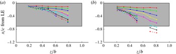
Here we analyse the LEV tilting, axial flow and vorticity flux. We visualize any aft LEV tilting with time by plotting
 $x$
-direction trajectories of the LEV centre from 20 % to 80 % span, in steps of 10 %, in figure 9. The trajectories are connected, coloured lines for each
 ${\it\phi}$
value, and outboard LEVs are only identified up to a certain
 ${\it\phi}$
. A top or (
 $x$
,
 $z$
)-plane view of the plate is shown and a grey region gives the projected plate area; the span scale is
 $z/b$
so that the plate spans have the same length. For each
 $\AR$
the LEV centre locations begin parallel to the leading edge as expected, then by
 ${\it\phi}=36^{\circ }$
there is substantial aft tilt and the LEV centre also shifts rearward as the vortex grows. Where the LEV is ‘stable’ for each
 $\AR$
, the tilt and trajectory variation with
 ${\it\phi}$
are smaller; the outboard tilt is much larger. The
 $\AR =4$
outboard LEV centre moves aft of the trailing edge at 70 % span for
 ${\it\phi}>36^{\circ }$
, and at 80 % span and
 ${\it\phi}=48^{\circ }$
it is
 ${\sim}0.2c$
past the trailing edge. Conversely, for
 $\AR =2$
at 80 % span and
 ${\it\phi}=60^{\circ }$
(highest angle with an identified LEV), the LEV centre position does not move past the trailing edge, indicating less tilt.
LEV centre
 $x$
-direction trajectories versus
 ${\it\phi}$
, top-view of plate: (a)
 $\AR =2$
; (b)
 $\AR =4$
. Data for
 ${\it\phi}=6{-}120^{\circ }$
, incrementing by
 ${\rm\Delta}{\it\phi}=6^{\circ }$
, are given by the colour progression: red, green, blue, yellow, magenta, cyan, black, which repeats but line styles also progress as solid, dashed, dash-dot, ending with cyan and dash-dot for
 ${\it\phi}=120^{\circ }$
. As described in the text, an outboard LEV is not found for all
 ${\it\phi}$
. LE: leading edge.

Substantial aft LEV tilt will reduce the spanwise LEV circulation, due to the conversion of some of the
 ${\it\omega}_{z}$
to streamwise vorticity
 ${\it\omega}_{x}$
. Kim & Gharib (Reference Kim and Gharib2010) and Ozen & Rockwell (Reference Ozen and Rockwell2012) also reported significant rearward LEV tilt and streamwise vorticity for their
 $\AR \approx 2$
wings. The LEV tilting over the entire span generally increases up to
 ${\it\phi}\approx 36^{\circ }$
, after which its evolution slows. This attainment of maximum tilt coincides with the reduction in slope of both
 ${\it\Gamma}_{\mathit{LEV}}^{\ast }$
and
 ${\it\Gamma}_{\mathit{total}}^{\ast }$
. However, after this the decrease in spanwise circulation due to tilting will not change significantly. An exception is the 70–80 % region for
 $\AR =4$
. The continued aft tilting here yields the lower
 ${\it\Gamma}_{\mathit{LEV}}^{\ast }$
at 70 % span compared with
 $\AR =2$
(figure 6
d).
Next we analyse the volume flow rate and vorticity flux along the LEV. We account for the LEV tilting by calculating an axial unit vector,
 ${\bf\beta}$
, which is parallel to the LEV centre axis. This is done using the information from figure 9, for each spanwise position and
 ${\it\phi}$
, again only when an LEV can be identified. For example, for a given
 ${\it\phi}$
, the
 ${\bf\beta}$
at 20 % span is taken to be the unit vector whose direction is parallel to the line connecting the LEV centre at 20 % span to that at 30 % span, with positive defined as outboard. Therefore, for a given spanwise location
 ${\bf\beta}$
is computed using the LEV (
 $x$
,
 $y$
,
 $z$
) centre position there and at 10 % span outboard. The
 ${\bf\beta}$
are not calculated at 80 % span, because no 90 % span LEV data are considered. The LEV axial velocity is defined at each grid point as the scalar product of the velocity vector and the axial unit vector,
 $\boldsymbol{u}_{axial}=(\boldsymbol{u}\boldsymbol{\cdot }{\bf\beta}){\bf\beta}$
. We define the non-dimensional vorticity flux as
 $(\boldsymbol{u}\boldsymbol{\cdot }{\bf\beta})|{\bf\omega}|=u_{axial}|{\bf\omega}|$
.
We first examine the non-dimensional volume flow rate, which is the area integral of the non-dimensional
 $u_{axial}$
over the non-dimensional LEV area; this is done for each identified LEV at the selected spanwise positions (
 $z/b$
) and for each
 ${\it\phi}$
. Note that Carr et al. (Reference Carr, Chen and Ringuette2013a
) showed both positive (outboard) and negative (inboard) spanwise velocity in the vicinity of the LEV for
 $\AR =2$
and 4, which was also found by e.g. Lu & Shen (Reference Lu and Shen2008), Jardin et al. (Reference Jardin, Farcy and David2012), Phillips & Knowles (Reference Phillips and Knowles2013) and Garmann & Visbal (Reference Garmann and Visbal2014). To gain insight into the individual contributions of the positive and negative
 $u_{axial}$
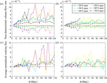
, we calculate the non-dimensional volume flow rate conditionally on its positive and negative components; this is given in figure 10(a,b) for
 $\AR =2$
and 4, respectively. The overall trend for each
 $\AR$
is that the positive non-dimensional LEV volume flow rates generally have greater magnitudes than the negative components. In addition, in some instances the magnitudes increase with greater spanwise position, particularly from 20 % to 50 % span and for the positive components. Further, the volume flow rate magnitudes for
 $\AR =2$
are typically larger than for
 $\AR =4$
. For both
 $\AR\text{s}$
, the volume flow rates at 50 % span (and 60 % for
 $\AR =2$
) exhibit substantial fluctuations for
 ${\it\phi}>48^{\circ }$
, due to breakdown.
Non-dimensional volume flow rate and average vorticity flux for the LEV, for 20–70 % span,
 $\AR =2$
(a,c) and
 $\AR =4$
(b,d). For the non-dimensional volume flow rate, solid lines indicate the calculation done conditionally using only positive volume flow rate regions, while the dashed lines similarly give it for negative regions.

The average non-dimensional LEV vorticity flux at different spanwise locations is shown for
 $\AR =2$
and 4 in figure 10(c,d), respectively. It is calculated as the area integral of the non-dimensional vorticity flux, divided by the LEV area. The positive and negative components of the average vorticity flux (not shown) have trends similar to the volume flow rate for each
 $\AR$
. As figure 10(c,d) demonstrate, the average vorticity flux is generally positive (outboard) for both
 $\AR\text{s}$
, except for a small number of fluctuations below 0. Unlike the volume flow rate, the vorticity flux values are comparable for each
 $\AR$
at a given spanwise position. For
 $\AR \approx 2$
, Kim & Gharib (Reference Kim and Gharib2010) also found primarily positive LEV vorticity flux (in this case, the area integral of the flux), while Ozen & Rockwell (Reference Ozen and Rockwell2012) showed positive flux when the LEV is concentrated and near the plate, but negative flux when the LEV is lifted away from the plate and grows longer aft. For
 ${\it\phi}\geqslant 36^{\circ }$
and between 30 % and 50 % span for both
 $\AR\text{s}$
, in some instances the vorticity flux increases with span, which Kim & Gharib (Reference Kim and Gharib2010) state indicates transport outboard toward the tip. This will also act to reduce
 ${\it\Gamma}_{\mathit{LEV}}^{\ast }$
.
In the LEV flow fields we observe patches of both positive and negative
 $u_{axial}$
, as found by others, however the spatial resolution of the present data sets does not allow for these to be fully resolved. We believe this is the explanation for the fluctuations observed in the curves of the non-dimensional volume flow rate and average vorticity flux; however, again for 50 % and 60 % span and
 ${\it\phi}>48^{\circ }$
, the larger fluctuations are due to breakdown.
3.2. Circulation in the tip region
To characterize the tip-region flow for
 $\AR =2$
and 4, we calculate the total circulation in vertical (
 $y$
,
 $z$
) planes aligned with the span, i.e. having constant
 $x$
-positions. This time-varying circulation,
 ${\it\Gamma}_{x}^{\ddagger }$
, is computed as the area integral of all of the negative streamwise (out-of-plane) vorticity,
 ${\it\omega}_{x}<0$
, which has the same sign as that of the TV. Only magnitudes above the vorticity threshold are included. This is shown for three planes in figure 11, one at mid-chord, one in the data plane just aft of the trailing edge, and one with an
 $x$
distance of
 $0.5c$
behind the trailing edge, to obtain information about the spatial distribution.
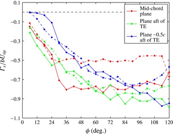
Plot of
 ${\it\Gamma}_{x}^{\ddagger }$
in three vertical (
 $y$
,
 $z$
) data planes, one at mid-chord, one in the data plane just aft of the trailing edge (TE), and one
 $0.5c$
behind the TE. Solid lines:
 $\AR =2$
, dashed:
 $\AR =4$
.

At mid-chord (red curves), the magnitude of
 ${\it\Gamma}_{x}^{\ddagger }$
for
 $\AR =4$
increases then essentially saturates after
 ${\it\phi}=30^{\circ }$
. For
 $\AR =2$
, there is similar behaviour but with saturation occurring for
 ${\it\phi}\geqslant 36^{\circ }$
. What is striking is that the magnitude of
 ${\it\Gamma}_{x}^{\ddagger }$
after saturation is much larger for
 $\AR =2$
, namely
 $|{\it\Gamma}_{x}^{\ddagger }|\approx 0.8$
, compared with
 $|{\it\Gamma}_{x}^{\ddagger }|\approx 0.5$
for
 $\AR =4$
. This stands out when considering that for the plane just behind the trailing edge (green curves) and
 $0.5c$
aft of the trailing edge (blue curves), the magnitudes for
 $\AR =2$
and 4 are much more similar.
Just behind the trailing edge, the
 ${\it\Gamma}_{x}^{\ddagger }$
curves for each
 $\AR$
have initially steeper slopes which gradually reduce and approximately level off for
 ${\it\phi}>72^{\circ }$
; this latter behaviour corresponds to the outboard breakdown of the flow near the trailing edge (figure 4). The magnitudes for
 $\AR =2$
are slightly larger in this region because the flow is more coherent. For the plane
 $0.5c$
aft of the trailing edge,
 $|{\it\Gamma}_{x}^{\ddagger }|$
for
 $\AR =2$
generally increases with
 ${\it\phi}$
until deceleration. Conversely, for
 $\AR =4$
the
 $|{\it\Gamma}_{x}^{\ddagger }|$
grows only up to
 ${\it\phi}=84^{\circ }$
, because unlike for
 $\AR =2$
the substantial flow breakdown eventually propagates aft past
 $0.5c$
behind the trailing edge (figure 4). The
 $|{\it\Gamma}_{x}^{\ddagger }|$
at
 $0.5c$
aft are generally smaller than those just behind the trailing edge, likely due to the tilting of the loop structure which converts some of the
 ${\it\omega}_{x}$
to
 ${\it\omega}_{z}$
.
Returning to the mid-chord location, the much lower
 $|{\it\Gamma}_{x}^{\ddagger }|$
for
 $\AR =4$
after saturation (
 ${\it\phi}\geqslant 30^{\circ }$
) is directly related to the loss of coherence of the tip-region flow. The
 $\AR =4$
iso-
 ${\mathcal{Q}}$
surfaces in figure 4 show that after the initial outboard LEV lift-off (
 ${\it\phi}=30^{\circ }$
) multiple, smaller LEVs form and convect past the plate, and also that the main TV moves aft behind the trailing edge, although a smaller region of tip vorticity remains just outside the tip (
 ${\it\phi}=48^{\circ }$
and 60°). This is followed by a transitional flow with massive outboard breakdown (
 ${\it\phi}=90^{\circ }$
). This flow evolution does not yield a coherent large-scale vortical structure which resides over the tip region, and the
 ${\it\Gamma}_{x}^{\ddagger }$
saturates at a low level. By comparison, the
 $\AR =2$
LEV lift-off is not progressive, and the aft-tilted LEV interacts and eventually merges with the TV (
 ${\it\phi}\geqslant 60^{\circ }$
). Even in the presence of breakdown, this yields a more coherent and perpetual vortical flow over the tip, which generates the higher level of mid-chord
 $|{\it\Gamma}_{x}^{\ddagger }|$
. This region of stronger and more coherent vortical flow will produce a relatively lower outboard pressure over the plate for
 $\AR =2$
, which should contribute to the
 $C_{L}$
as discussed in § 3.4.
3.3. Lift force
The force transducer measurements are non-dimensionalized using a conventional lift coefficient defined as
 $$\begin{eqnarray}C_{L}\equiv \frac{L}{\displaystyle ({\textstyle \frac{1}{2}}{\it\rho}U_{\mathit{tip}}^{2})A_{plate}},\end{eqnarray}$$
where
 $A_{plate}=cb$
is the plate area. Figure 12 plots the
 $C_{L}$
for
 $\AR =1{-}4$
with
 ${\it\phi}_{\mathit{final}}=120^{\circ }$
(for
 $\mathit{Re}_{\mathit{span}}=1300{-}21\,500$
) and 360° (for
 $\mathit{Re}_{\mathit{span}}\approx 5780\AR$
). The abscissa is time normalized by the
 ${\it\phi}_{\mathit{final}}=120^{\circ }$
period,
 $t/T_{120^{\circ }}$
; the deceleration portions are not shown. There is clearly an insensitivity of
 $C_{L}$
to
 $\mathit{Re}$
(for the range tested), which is maintained throughout the plate motion. All cases have a
 $C_{L}$
peak from non-circulatory force during acceleration, which increases with decreasing
 $\AR$
due to higher rates required to match
 $\mathit{Re}$
; variations in peak
 $C_{L}$
with
 $\mathit{Re}$
are due mostly to signal filtering. The acceleration causes some persisting mechanical vibrations in the force signal; for decreasing
 $\AR$
, these are increasingly artificially amplified by the normalization using the plate area. Next is a gradual growth phase to
 $t/T_{120^{\circ }}\approx 0.7$
, where the
 $C_{L}$
variation with
 $\AR$
is reduced substantially, which is then followed by a leveling off (see also Sun & Wu Reference Sun and Wu2004; Schlueter et al.
Reference Schlueter, Jones, Granlund and Ol2013). The large-time behaviour indicates a slight decrease in
 $C_{L}$
with increasing
 $\AR$
.
Lift coefficient,
 $C_{L}$
, for
 ${\it\phi}_{\mathit{final}}=120^{\circ }$
(solid lines, all
 $\mathit{Re}$
cases) and
 ${\it\phi}_{\mathit{final}}=360^{\circ }$
(dashed lines,
 $\mathit{Re}_{\mathit{span}}\approx 5,780\AR$
). Time is normalized by the period of the
 ${\it\phi}_{\mathit{final}}=120^{\circ }$
cases. Left inset: average lift,
 $L_{\mathit{avg}}$
, after acceleration phase. The curves are proportional to
 $U_{\mathit{tip}}^{2}$
. Right inset: lift coefficient corresponding to the left inset.

Although figure 12 shows minor variations of
 $C_{L}$
with
 $\mathit{Re}$
and
 $\AR$
, it is worthwhile to consider how these parameters may affect the lift coefficient. The variation of
 $C_{L}$
with
 $\AR$
depends on the way in which
 $\AR$
itself is varied; for example, whether the chord or span is varied (or both). This is because
 $\AR$
,
 $\mathit{Re}$
and
 $C_{L}$
are implicitly linked, which complicates the physical interpretation of
 $C_{L}$
variations. For this reason we first focus on the dimensional lift and the associated physics. In general,
 $L$
is a function of
 $\mathit{Re}$
and
 $\AR$
, and we assume that this functionality may be written as a separable product of functions:
 $$\begin{eqnarray}L=f(\mathit{Re})g(\AR).\end{eqnarray}$$
To estimate these functions we compute an average lift,
 $L_{\mathit{avg}}$
, using the measured force data during the constant velocity phase of the motion (
 $t/T_{120^{\circ }}\approx 0.2$
–0.8). This
 $L_{\mathit{avg}}$
is plotted against the characteristic velocity for each case,
 $U_{\mathit{tip}}$
, in the left inset of figure 12 and shows that the dimensional lift is proportional to
 $U_{\mathit{tip}}^{2}$
. This result is not surprising and is consistent with classical aerodynamics, in which use of the dynamic pressure in the definition of
 $C_{L}$
collapses this dependence on
 $U_{\mathit{tip}}$
. Furthermore, for a given
 $\AR$
(and fluid) we have
 $L\propto U_{\mathit{tip}}^{2}\propto \mathit{Re}^{2}$
meaning that
 $f(\mathit{Re})\sim \mathit{Re}^{2}$
, which explains why the
 $C_{L}$
in figure 12 show no significant dependence on
 $\mathit{Re}$
.
It now remains to determine the dependence of the dimensional lift on
 $\AR$
, which is represented by the function
 $g(\AR)$
in (3.2). For a fixed value of
 $U_{\mathit{tip}}$
it is quite reasonable to assume that lift will increase with increasing plate area. However, the area can be written as
 $$\begin{eqnarray}A_{plate}=c^{2}\AR =b^{2}\AR^{-1}.\end{eqnarray}$$
Hence, if the chord is held constant and
 $\AR$
is changed through varying the span, then the area and lift will increase/decrease with increasing/decreasing
 $\AR$
. For constant span and variable chord, the opposite is true and lift will decrease/increase with increasing/decreasing
 $\AR$
. The current experiments belong to the former case, as can be verified by comparing the data for the different
 $\AR\text{s}$
in the
 $L_{\mathit{avg}}$
versus
 $U_{\mathit{tip}}$
plot in figure 12.
Although we have the general trend of dimensional lift with varying
 $\AR$
, the actual form of
 $g(\AR)$
is unknown. If we consider
 $g(\AR)$
to have dimensions of area (making
 $f(\mathit{Re})$
a pressure), then we can interpret this function as the effective lift-producing area of the plate. The behaviour of
 $C_{L}$
with
 $\AR$
is then governed by the ratio
 $g(\AR)/A_{plate}$
. For the current experiments (constant
 $c$
, variable
 $b$
), we use the measurements to estimate how
 $g(\AR)$
increases with
 $\AR$
. A least-squares fit to the data yields
 $g(\AR)\propto c^{2}\AR$
(with an
 $R^{2}=0.9965$
) in the
 $\AR$
range investigated, and with
 $A_{plate}=c^{2}\AR$
the lift coefficient is then nominally constant. The computations of Luo & Sun (Reference Luo and Sun2005) and Harbig et al. (Reference Harbig, Sheridan and Thompson2013) also showed little variation in
 $C_{L}$
for
 $\AR\text{s}$
overlapping the present
 $\AR$
range. The right inset of figure 12 plots the lift coefficient corresponding to
 $L_{\mathit{avg}}$
, that is
 $C_{L,\mathit{avg}}$
, showing this behaviour, which obviously agrees with the time traces of the
 $C_{L}$
(after the acceleration phase). This same analysis can be applied to plates with constant
 $b$
and variable
 $c$
, but measurements of this type of
 $\AR$
variation are required to determine the actual
 $g(\AR)$
and hence
 $C_{L}$
. The force transducer measurements represent an integrated or global quantity, and hence no local information is obtained. As such, there may be
 $\AR$
effects contained within the flow structures that contribute to the lift; this is discussed in the following section.
3.4. Vortex structure and lift
Here, we use the S-DPIV data to seek out possible effects of
 $\AR$
on
 $C_{L}$
by appealing to the corresponding vortex structures generated by the plates. Wu (Reference Wu1981) gives a formula for the force on a body moving in an infinite three-dimensional region of incompressible fluid as
 $$\begin{eqnarray}\boldsymbol{F}(t)=-\frac{1}{2}{\it\rho}\frac{\text{d}}{\text{d}t}\int _{V_{\infty }}\boldsymbol{x}\times {\bf\omega}\text{d}V+{\it\rho}\frac{\text{d}}{\text{d}t}\int _{V_{b}}\boldsymbol{u}\text{d}V,\end{eqnarray}$$
where
 ${\it\rho}$
is the fluid density and
 $\boldsymbol{x}$
is position. It should be noted here that the finite measurement volume technically invalidates the use of (3.4). However, the flow structure is contained within the volume for at least the first half of the plate motion and the contributions due to a finite control surface only become significant later in the motion (see DeVoria, Carr & Ringuette Reference DeVoria, Carr and Ringuette2014). We opt for this simplified equation to ease the following discussion (Noca, Shiels & Jeon (Reference Noca, Shiels and Jeon1999) gave formulas for a body that is contained within a finite control surface).
The first integral term in (3.4) is the rate of change of the total first moment of vorticity and is over the volume
 $V_{\infty }$
which includes the fluid,
 $V_{f}$
, and the body,
 $V_{b}$
. The next term is the inertial force of the fluid displaced by
 $V_{b}$
. This latter term has zero contribution to the lift, because the rotation plane and
 $y$
-axis are orthogonal. We first investigate the lift-direction component of the vorticity-moment integral, that is the (hydrodynamic) lift impulse,
 $P_{L}$
, before computing lift from the S-DPIV data. For pure rotation, the following
 $P_{L}$
equation applies to any rotating coordinate system (
 $x^{\prime }$
,
 $y^{\prime }$
,
 $z^{\prime }$
) with
 $y^{\prime }=y$
:
 $$\begin{eqnarray}\displaystyle & \displaystyle P_{L}=\left(-\frac{1}{2}{\it\rho}\int _{V_{f}}z{\it\omega}_{x}\text{d}V\right)+\left(\frac{1}{2}{\it\rho}\int _{V_{f}}x{\it\omega}_{z}\text{d}V\right)\equiv P_{L,z{\it\omega}_{x}}+P_{L,x{\it\omega}_{z}}, & \displaystyle\end{eqnarray}$$
 $$\begin{eqnarray}\displaystyle & \displaystyle P_{L}^{\ast }\equiv P_{L}\Big/\left\{\frac{1}{2}{\it\rho}U_{tip,max}^{2}cbT\right\}=\int C_{L}\text{d}\!\left(\frac{t}{T}\right), & \displaystyle\end{eqnarray}$$
 $P_{L,z{\it\omega}_{x}}$
) and spanwise (
 $P_{L,x{\it\omega}_{z}}$
) vorticity. Also,
 $P_{L}^{\ast }$
is the lift impulse coefficient and
 $T$
is the motion duration. We use the ‘objective origin’ method of DeVoria et al. (Reference DeVoria, Carr and Ringuette2014) to determine a position vector origin that minimizes the errors in the impulse calculation associated with amplification of the velocity measurement noise.
Figure 13(a) shows
 $P_{L}^{\ast }$
versus
 ${\it\phi}$
from the transducer, as well as
 $P_{L,z{\it\omega}_{x}}^{\ast }$
and
 $P_{L,x{\it\omega}_{z}}^{\ast }$
from the S-DPIV data for
 $\AR =2$
and 4. In general, both
 $P_{L,z{\it\omega}_{x}}^{\ast }$
and
 $P_{L,x{\it\omega}_{z}}^{\ast }$
steadily increase, agreeing with the transducer data. For both
 $\AR\text{s}$
, the streamwise vorticity moment contribution changes slope and increases more rapidly starting at
 ${\it\phi}\approx 72^{\circ }$
. This is associated with both the tilt of the LEV (see figure 9) and breakdown, which disperses the vortex structure at the plate tip (see figure 4). For
 $\AR =4$
the spanwise vorticity moment contribution suddenly decreases, because of vorticity loss corresponding to the TEV leaving the measurement volume. However, the orientation of the TEV at this time is such that it also contains streamwise vorticity and there is vorticity loss in
 $P_{L,z{\it\omega}_{x}}^{\ast }$
, as well. These effects are not as severe for
 $\AR =2$
, for which
 $P_{L,x{\it\omega}_{z}}^{\ast }$
continues to increase due to breakdown also dispersing spanwise vorticity.
(a) Lift impulse coefficients from the transducer and the contributions
 $P_{L,z{\it\omega}_{x}}^{\ast }$
and
 $P_{L,x{\it\omega}_{z}}^{\ast }$
from S-DPIV. These cases correspond to
 $\mathit{Re}\approx 10\,600$
,
 ${\it\phi}_{\mathit{final}}=120^{\circ }$
. (b) The lift coefficients of the S-DPIV data shown in plot (a).

To better interpret
 $P_{L,z{\it\omega}_{x}}$
and
 $P_{L,x{\it\omega}_{z}}$
in the context of particular vortex structures and their circulations, consider the overall vortex structure to be a single loop segment with attachment points on the plate, which act as vorticity sources allowing a variable circulation,
 ${\it\Gamma}(\ell )\geqslant 0$
, along the loop. If
 $\text{d}\boldsymbol{\ell }$
is a differential loop segment, then
 $$\begin{eqnarray}-\int \boldsymbol{x}\times {\bf\omega}\text{d}V=-\oint \boldsymbol{x}\times {\it\Gamma}(\ell )\text{d}\boldsymbol{\ell }.\end{eqnarray}$$
Writing
 $\text{d}\boldsymbol{\ell }={\bf\tau}\text{d}\ell$
, with
 ${\bf\tau}={\bf\omega}/|{\bf\omega}|$
, and considering the lift direction, the above becomes
 $$\begin{eqnarray}\oint [x_{v}({\it\Gamma}{\it\tau}_{z})-z_{v}({\it\Gamma}{\it\tau}_{x})]\text{d}\ell =\oint [(x_{v}{\it\Gamma}{\it\tau}_{z})_{\mathit{LEV}}+(x_{v}{\it\Gamma}{\it\tau}_{z})_{TEV}-(z_{v}{\it\Gamma}{\it\tau}_{x})_{TV}-(z_{v}{\it\Gamma}{\it\tau}_{x})_{RV}]\text{d}\ell ,\end{eqnarray}$$
where the
 ${\it\tau}$
are direction cosines representing the (local) vortex tilt,
 $x_{v}$
and
 $z_{v}$
are the streamwise and spanwise vortex positions, and the right-hand side has split the integrand into circuit segments along the LEV, TEV, TV and RV. An origin may be chosen such that
 $x_{v,\mathit{LEV}}\approx -x_{v,TEV}\equiv x_{v}>0$
and
 $z_{v,TV}\approx -z_{v,RV}\equiv z_{v}>0$
. For the LEV,
 ${\it\tau}_{z}>0$
and we let
 ${\it\tau}_{\mathit{LEV}}={\it\tau}_{z,\mathit{LEV}}$
; similarly, let
 ${\it\tau}_{TEV}=-{\it\tau}_{z,TEV}$
,
 ${\it\tau}_{TV}=-{\it\tau}_{x,TV}$
and
 ${\it\tau}_{RV}={\it\tau}_{x,RV}$
, each of which are positive, giving
 $$\begin{eqnarray}\frac{1}{2}\oint x_{v}[({\it\Gamma}{\it\tau})_{\mathit{LEV}}+({\it\Gamma}{\it\tau})_{TEV}]\text{d}\ell +\frac{1}{2}\oint z_{v}[({\it\Gamma}{\it\tau})_{TV}+({\it\Gamma}{\it\tau})_{RV}]\text{d}\ell \approx P_{L,x{\it\omega}_{z}}+P_{L,z{\it\omega}_{x}}.\end{eqnarray}$$
Taking the time derivative of the above equation shows that the lift will increase if the circulation of any of the vortex segments grows, and if the vortex loop size increases. As mentioned above, the vorticity loss makes any of the above impulse equations invalid. For this reason, we only use the lift impulse data prior to the vorticity loss to compute lift coefficients from the S-DPIV data, namely
 $C_{L,z{\it\omega}_{x}}$
and
 $C_{L,x{\it\omega}_{z}}$
. The impulse data are lightly smoothed to avoid degrading the signal with numerical differentiation.
The lift coefficients corresponding to the two terms in (3.5) are plotted in figure 13(b), and we note that these contributions may be quantitatively compared across each
 $\AR$
since there is small variation of the total
 $C_{L}$
with
 $\AR$
. The
 $C_{L,x{\it\omega}_{z}}$
contributions to lift are fairly close for both
 $\AR\text{s}$
early on. This suggests that the LEV and TEV provide the same relative lift contributions independent of
 $\AR$
, which is supported by the similarity of the flow structure at small rotation angles. Also, the initial decrease of
 $C_{L,x{\it\omega}_{z}}$
reveals that the TEV significantly affects
 $C_{L}$
up to
 ${\it\phi}\approx 30^{\circ }$
, where
 $C_{L,x{\it\omega}_{z}}$
(temporarily) levels off as the TEV is advected away. Figure 6(b) shows that this rotation angle also coincides with the leveling off of the first LEV circulation for both
 $\AR\text{s}$
. However, the
 $C_{L}$
were observed to continue to gradually increase (recall figure 12), which can be explained by the increase of
 $C_{L,x{\it\omega}_{z}}$
from
 ${\it\phi}\approx 36^{\circ }$
to
 $60^{\circ }$
. This implies that the cessation of any Wagner-type effects essentially coincides with the first LEV saturation. Since the TEV is no longer influencing
 $C_{L}$
at these angles,
 $C_{L,x{\it\omega}_{z}}$
can be interpreted as the lift contribution from all LEVs. Figure 5(b) shows that the total spanwise circulation also gradually continues to grow, but recall that the first LEV circulation has saturated. This means that the increased lift is associated with the secondarily generated LEVs. For
 $\AR =2$
,
 $C_{L,x{\it\omega}_{z}}$
begins to decrease after
 ${\it\phi}=60^{\circ }$
because of breakdown. Based on the matching behaviours of
 $C_{L,x{\it\omega}_{z}}$
for both
 $\AR\text{s}$
prior to this time, it is likely that breakdown also reduces the
 $C_{L}$
contribution of the LEVs for the
 $\AR =4$
case as well. However, due to the vorticity loss, we cannot make a confident assertion.
Consider now the contribution from
 $C_{L,z{\it\omega}_{x}}$
, which represents the lift coefficient corresponding to the TV. Although the RV is not captured in the S-DPIV measurements, this structure is of negligible strength compared with the remaining vortices. Figure 13(b) shows that
 $C_{L,z{\it\omega}_{x}}$
generally increases for
 $\AR =2$
, while it decreases for
 $\AR =4$
. This implies that the
 $C_{L}$
for low
 $\AR$
has a larger TV contribution, whereas for higher
 $\AR$
this contribution is decreased. Furthermore, for
 $\AR =2~C_{L,z{\it\omega}_{x}}$
is consistently larger than
 $C_{L,x{\it\omega}_{z}}$
over the majority of the data shown, and the two show cooperative behaviours up to
 ${\it\phi}\approx 60^{\circ }$
. For
 $\AR =4$
, the decrease in the effectiveness of the TV is related to the aft location of the TV as discussed in § 3.1.1.
4. Concluding remarks
We use experiments to investigate the effect of
 $\AR$
on the vortex structure and circulation, and their relationship to the lift force, for flat-plate wings rotating from rest at 45° angle of attack. This configuration is a simplified model of a hovering-wing half-stroke. We also examine
 $\mathit{Re}$
effects on the lift coefficient for
 $\mathit{Re}_{\mathit{span}}$
of
 $O(10^{3}{-}10^{4})$
. The flow quantities are acquired for
 $\AR =2$
and 4 using phase-locked, phase-averaged S-DPIV volume reconstructions with nearly matching
 $\mathit{Re}_{\mathit{span}}=10\,700$
and 10 433, respectively, and the unsteady lift is directly measured for
 $\AR =1{-}4$
. The goal is to obtain a better understanding of
 $\AR$
, or tip, effects by analysing the spatiotemporal circulation of both the LEV and tip region, obtaining
 $C_{L}$
versus
 $\AR$
, and connecting the flow quantities and forces by calculating the lift-impulse coefficient and
 $C_{L}$
from the S-DPIV.
We characterize the spatiotemporal development of the total leading-edge region spanwise circulation by identifying normalizations suitable for comparing different
 $\AR\text{s}$
. Normalizing its magnitude by the plate span and comparing its evolution for matching rotation angle
 ${\it\phi}$
produces the closest magnitudes and trends for
 $\AR =2$
and 4, for the
 ${\it\phi}_{\mathit{final}}=120^{\circ }$
rotation tested. However, early in the motion before plate end-effects become important, the circulation is better characterized by the local chord lengths travelled. The total circulation increases with span and peaks in the tip region, and is larger for
 $\AR =2$
. Normalizing the circulation using the local azimuthal velocity at each spanwise position, rather than that at the tip, substantially reduces the variation with span except near the plate ends, allowing for spanwise averages. The span-averaged total circulation plotted against
 ${\it\phi}$
has an initially large slope for each
 $\AR$
, then the growth rate slows but remains positive; after the startup, the slopes are very similar for
 $\AR =2$
and 4.
Volumetric renderings of the vortical structure using isosurfaces of the
 ${\mathcal{Q}}$
-criterion show an overall LEV–TV–TEV vortex loop, and an arch-like lift-off of the outboard LEV for each
 $\AR$
, followed by further smaller LEVs. Afterward, for
 $\AR =4$
the tip-region flow becomes less coherent and the outboard LEV and TV move aft off the plate. Conversely, for
 $\AR =2$
the aft-tilted LEV merges with the TV to create a more coherent structure that consistently resides over the tip. Both
 $\AR\text{s}$
exhibit outboard LEV and TV breakdown, which is more pronounced for
 $\AR =4$
. This coincides with an increase in the outboard LEV core size, and the breakdown creates small, unorganized vortical structures in the volume rendering due to the flow non-repeatability.
Where the first LEV is ‘stable’ inboard, its spanwise circulation saturates for
 $\AR =2$
after
 ${\it\phi}\approx 30^{\circ }$
, and similarly the growth of the
 $\AR =4$
LEV circulation then slows considerably. The LEV generally tilts increasingly aft until
 ${\it\phi}\approx 36^{\circ }$
; the tilt for the ‘stable’ LEV is much less than outboard. The LEV tilt is responsible for a reduction in the spanwise circulation as spanwise vorticity is converted to streamwise. Near the tip, the
 $\AR =4$
LEV tilt progresses and yields lower spanwise circulation. The LEV exhibits both positive and negative non-dimensional axial volume flow rate, although the positive components are typically larger. Correspondingly, the average LEV vorticity flux is generally positive.
The circulation due to streamwise (tip-region) vorticity is obtained in vertical, span-parallel planes. At the plate mid-chord position, it grows then saturates for both
 $\AR\text{s}$
. The mid-chord saturation level is considerably smaller for
 $\AR =4$
, due to the absence of organized, large-scale vortices over the tip. The stronger and more coherent tip-region vortices for
 $\AR =2$
will lead to a comparatively lower-pressure region above the plate, producing a larger contribution to the overall lift. Aft of the plate, the circulation magnitudes are more similar.
When varying
 $\AR$
from 1 to 4 by maintaining a constant chord length, the average
 $C_{L}$
from the transducer measurement during the unsteady growth phase (after acceleration) is essentially constant with
 $\AR$
; the
 $C_{L}$
is insensitive to
 $\mathit{Re}$
for the range tested. The long-time behaviour shows a slight decrease in
 $C_{L}$
with increasing
 $\AR$
.
The transducer data do not yield local information on how the flow structures contribute to the lift force for varying
 $\AR$
. Therefore, to examine any
 $\AR$
effects on these contributions, we calculate the streamwise and spanwise components of the lift-impulse directly from the volumetric flow data. We employ a simplified LEV–TV–TEV–RV loop model to show that the impulse increases when the circulation of any of these vortices grows, or when the loop size increases. We compute the spanwise and streamwise components of the
 $C_{L}$
from the impulse data. The spanwise component, which includes contributions from the TEV and LEV structures, is similar for
 $\AR =2$
and 4. This reflects their comparable TEV interactions and LEV saturation or slow-growth behaviour, and their very similar slopes for the time-varying total circulation; the latter is due to the formation of further LEVs outboard. However, the streamwise contribution to the
 $C_{L}$
for
 $\AR =2$
is much larger, due to the more coherent tip-region flow, which includes the stronger TV and aft-tilted LEV. As mentioned earlier, this flow will create a relatively lower-pressure region over the wing. Therefore, although the average
 $C_{L}$
for
 $\AR =2$
and 4 is essentially the same, it is arrived at via different contributions from the flow structures. Moreover, the large-time trend of the
 $C_{L}$
decreasing slightly with
 $\AR$
, beyond where our S-DPIV data are available, is likely the result of the more coherent tip flow for lower
 $\AR$
.
The main contribution of the present paper is the analysis of the spatiotemporal leading-edge and tip-region circulation, and through this and the force information, the demonstration that the flow structures contribute differently to the lift for varying
 $\AR$
. Further, we find very good agreement of the present volumetric flow structures with previous computations and experimental data, cited above, and in the LEV circulation trends with time and
 $\AR$
from the available data sets.
These results indicate that the influence of the wing-tip flow for lower
 $\AR$
is beneficial for lift production. However, the lift-to-drag ratio or efficiency was not examined and should be considered from an MAV design standpoint. Understanding the effects of wing geometry, particularly near the tip, as well as wing flexibility, on the above conclusions requires further study. Also, more work is needed in the area of low-order modelling for rotating and flapping wings, to capture the effects shown here and predict performance.
Acknowledgements
The authors wish to thank the anonymous reviewers for their time and very helpful suggestions for increasing the impact of this paper. We also thank M. Burge and J. Favale for assistance with the new
 $\AR =4$
S-DPIV measurements. This work was supported by the United States Air Force Office of Scientific Research, grant FA9550-10-1-0281, under the supervision of Dr D. Smith, and by the National Science Foundation, award no. 1336548, supervised by Dr D. Papavassiliou.