Introduction
The desire to gain a more integrated understanding of the visual system has popularized the rodent model in vision research. The rodent facilitates this understanding by permitting the study of genes, physiology, and behavior with the same organism. The mouse has captured most attention due to the ease with which its genome can be manipulated. However, its small size can present experimental limitations. The rat is advantageous in this regard and has proven useful for investigating a myriad of ocular diseases (Morrison et al., Reference Morrison, Moore, Deppmeier, Gold, Meshul and Johnson1997; Yu et al., Reference Yu, Cringle, Su, Yu, Jerums and Cooper2001; Chader, Reference Chader2002). Methodological advances in targeted gene manipulation promise to further enhance its appeal for vision research (Kitada et al., Reference Kitada, Ishishita, Tosaka, Takahashi, Ueda, Keng, Horie and Takeda2007).
A current drawback of the rat model is that comparatively little is known about the visual response properties of its retinal ganglion cells (RGCs), or whether the animal even possesses all the RGC types commonly found in other mammals. Such knowledge is fundamental to relating neural function to visual behavior under normal and pathophysiological conditions, as these cells are the sole messengers of visual information to the brain. It is also relevant to studies of higher cognitive centers since many behavior paradigms assess learning and memory via the ability of rats to perform visual tasks. What is known about the retinal representation of visual information comes from a handful of studies, which show that rat RGCs have center-surround receptive fields (RFs) with ON- or OFF-type centers that are large compared to those of cat and primate RGCs (Brown & Rojas, Reference Brown and Rojas1965; Partridge & Brown, Reference Partridge and Brown1970; Powers & Green, Reference Powers and Green1978; Anishchenko et al., Reference Anishchenko, Greschner, Elstrott, Sher, Litke, Feller and Chichilnisky2010). The studies did not evaluate findings against known physiological classification schemes, so homologies with canonical X-, Y-, or W-cell types have not been established. There is indirect evidence though for three major groups and several subgroups of rat RGC based on soma size (Fukuda, Reference Fukuda1977; Martin, Reference Martin1986), dendritic stratification pattern (Perry, Reference Perry1979; Dreher et al., Reference Dreher, Sefton, Ni and Nisbett1985; Huxlin & Goodchild, Reference Huxlin and Goodchild1997; Sun et al., Reference Sun, Li and He2002), and axon conduction velocity (Sefton & Swinburn, Reference Sefton and Swinburn1964; Fukuda, Reference Fukuda1977). One group has large somas and large dendritic trees analogous to alpha RGCs. These cells exhibit Y-type physiology in other mammals, which is characterized by brisk-transient responses, fast spike conduction, large RFs, and nonlinear spatial summation (reviews: Shapley & Perry, Reference Shapley and Perry1986; Levick, Reference Levick1996). The other two classes have small somas and either small or medium-large dendritic trees that resemble various subclasses of gamma RGCs and to some extent beta RGCs. Gamma cells exhibit W-type physiology in other mammals, which includes generally sluggish responses, slow spike conduction, and heterogeneous RF sizes and properties, while beta cells exhibit X-type physiology, which is associated with brisk-sustained responses, intermediate conduction speed, small RFs, and linear spatial summation (review: Troy & Shou, Reference Troy and Shou2002). Additional indirect evidence for multiple RGC types can be found in recordings from rat lateral geniculate nucleus (LGN) and pretectum (Fukuda et al., Reference Fukuda, Sumitomo, Sugitani and Iwama1979; Hale et al., Reference Hale, Sefton and Dreher1979; Lennie & Perry, Reference Lennie and Perry1981; Trejo & Cicerone, Reference Trejo and Cicerone1984; Prévost et al., Reference Prévost, Lepore and Guillemot2007). None of these studies identified a subcortical cell type with small RFs, but one did describe a few LGN cells that showed linear spatial summation (Lennie & Perry, Reference Lennie and Perry1981). Available data thus suggest that the rat retina may contain Y- and multiple W-type cells, while the support for X-type cells is mixed.
Here we provide a quantitative description of the spatial RF properties of rat RGCs. To do this, we outline a novel approach of simulating a spherical stimulus display, which corrects the nontrivial effect of planar distortions on patterns displayed at short viewing distances that has been neglected by in vivo studies of rodent vision. By exploring the individual behavior of each cell, multiple physiological types could be identified, including some rarely encountered types and one not previously described. The results show that rat RGCs have several RF properties in common with X-, Y-, and W-cell counterparts in cat, but there are also some notable differences, which challenge the functional roles these cell types are thought to fulfill in vision.
Materials and methods
Experimental preparation
Male retired breeder Brown Norway rats (300–400 g) were used for all experiments. In initial studies, statistically similar RF size measurements were collected from a small sample (n = 8) of RGCs in retired breeder Long-Evans rats. Details of the experimental preparation are reported elsewhere (Freeman et al., Reference Freeman, Heine and Passaglia2010). In short, rats were anesthetized with an intraperitoneal injection of ketamine hydrochloride (100 mg/kg) and xylazine (5 mg/kg). A catheter was then inserted into the femoral vein for intravenous drug delivery, and a tracheotomy was performed for mechanical ventilation during paralysis. An intramuscular injection of dexamethasone (1 mg) was delivered to minimize edema. The eyes were instilled with atropine sulfate, and the corneas were covered with artificial pupils (diameter: 1 mm). The head was rigidly fixed in a stereotaxic device, and a craniotomy was performed by drilling a 5 mm hole at bregma. After completion of all surgical procedures, the animal was maintained at an anesthetic plane for the remainder of the experiment via an intravenous infusion of ketamine (30 mg/kg/h), xylazine (1.5 mg/kg/h), and gallamine triethiodide (40 mg/kg/h) in saline supplemented with dextrose. Contrary to reports (Calderone et al., Reference Calderone, Grimes and Shalev1986), xylazine did not cause clouding of the lenses. Heart rate was monitored with an electrocardiogram and expired carbon dioxide with a capnometer. Body temperature was maintained at 37°C by a control unit connected to an anal thermistor and a heating blanket. A tungsten-in-glass microelectrode (tip length: 5–15 μm) was then inserted in a metal guide needle, which doubled as the reference electrode, and lowered into the brain at or near bregma until rhythmic activity was detected in response to periodic visual stimulation. This location placed the electrode in the optic chiasm or base of the optic tract. Spike times were stamped by a digital spike discriminator with a sampling rate of 10 kHz (Acquistion Processor Module; FHC Inc., Bowdoin, ME). After the experiment, the animal was euthanized via an overdose of Euthasol® (Virbac AH Inc., Ft.Worth, Tx). All experimental procedures were approved by Boston University Animal Care and Use Committee.
Visual stimulation
Visual stimuli were displayed on a cathode ray tube monitor (Sony Multiscan 17se, New York, NY, 30.2 × 40.4 cm2) with a frame rate of 100 Hz (noninterlaced) and mean luminance of 30 cd/m2. Custom software (Matlab, LabVIEW, Psychophysics Toolbox) controlled the monitor output. The stimulus set consisted of achromatic spots, annuli, and gratings, which the animal viewed at a distance of 16.5 cm from the cornea. The monitor could be moved laterally along a 200 deg arc, so that the screen could stimulate either eye. It was perpendicular to the optic axis of recorded neurons in the horizontal plane and fixed in the vertical plane at a height that positioned the eye 11.5 cm above the bottom of the screen in order to accommodate the disproportionate sampling of the mid-to-upper visual field by the rat eye. Since the screen is flat, a circular RF projected onto the monitor at this viewing distance will retain a circular shape near the optical center (15.1 cm from the side, 11.5 cm from the bottom) but appear elliptical toward screen edges. The confounding effects of a flat screen were minimized by simulating a spherical display centered on the optic axis of recorded cells.
To simulate a spherical display, the location of a pixel on the screen was specified by the vector P = (X, Y, Z), where X, Y, and Z are Cartesian coordinates referenced to the optical center point O defined by the pixel that is closest to the eye (Fig. 1a). Z was 16.5 cm for our setup. For a RF located at O, a sinusoidal grating must become curvilinear toward the screen margins in order for it to appear linear to the cell. This is accomplished for a vertical grating by the equation:

Spherical grating stimulus. (a) Coordinate space for mapping the visual display onto an imaginary spherical surface, with the displayed pattern centered about the RF of a cell located at (Cx , Cy ). The (0,0) coordinate marks the location O on the display, which is at eye level to the rat and introduces minimal distortion. (b) Two orientations of a spherical grating stimulus (left and right panels) as they would look on the display for a cell with a RF aimed at point O (crosshairs, top panels) and a point in the upper right corner (crosshairs, bottom panels). (c) Response profiles mapped with spherical (circles) and planar (squares) drifting gratings of various orientations with the RF of the same RGC positioned at three locations (dots). F1 amplitudes are specified for each grating orientation by the distance and phase angle of data points relative to the central dots. The inset plots the three spherical datasets with error bars, showing that the measured profiles did not depend on RF location in display space.

where L P is the luminance of pixel P, l is mean luminance, m is grating contrast, and k is grating spatial frequency in units of cycles per deg (cpd). For a cell with a RF located at C = (CX , CY , Z), the center point of the pattern must be shifted into alignment with the optic axis of the cell. This amounts to a rotation of the Z axis θ degrees horizontally and then φ degrees vertically, where

A pixel location in the rotated coordinate system becomes P′ = R(θ,φ) × P, where

For a different grating orientation ψ, the rotation matrix is:

To reduce the amount of planar correction, the RF of recorded cells was horizontally centered on the screen by sliding the monitor laterally until the first-harmonic (F1) response to counterphase modulation of a vertical bipartite field went through a null. At this location, the two halves of the RF center are equally and oppositely illuminated (i.e., CY = Y). The vertical position of the RF (CX ) was located in a similar manner by displacing a horizontal bipartite field up the screen. The simulator then generated spots, annuli, and grating patterns of desired characteristics given the measured optic axis of the cell (Fig. 1b), with pattern contrast defined in Michelson contrast units. The simulation accuracy was validated in two ways (Fig. 1c). First, RF center profiles measured with linear and curvilinear gratings were virtually identical for cells located at optical center. Second, the profile shape was preserved with curvilinear gratings if the RF of these cells was displaced toward screen edges (inset, two-way analysis of variance: F(12,42) = 1.6, P = 0.13). The RF location of each cell was periodically checked during data collection for possible eye movement and was not found to drift under the anesthetic and paralytic infusion rates used.
RF measurement
RF profiles were mapped via spatial tuning curves and spot response functions. Spatial tuning curves were measured by varying the spatial frequency of a full-field sine wave grating presented in 15 s epochs at a temporal frequency of 2 Hz, which is near optimal for rat RGCs. Spike trains were converted to peristimulus time histogram (PSTHs) by dividing the epochs into 0.5 s segments, binning at 128 Hz, and averaging across segments the spike count in each bin. Mean (F0), first-harmonic (F1), and second-harmonic (F2) temporal response amplitudes were then computed by Fourier analysis of the PSTHs. Grating contrast was adjusted across epochs so as to produce F1 responses within a linear range (<10 impulses/s, ips, Fig. 4). Cell responsivity (R) was defined by the average amplitude to contrast ratio (ips/contrast, ipsc) for three epochs in the linear response range. Spot response functions were mapped by varying the diameter of a sinusoidally modulated spot and calculating R in the same way. Since these are fixed-response (as opposed to fixed-contrast) paradigms, both datasets can be considered devoid of spike-rate nonlinearities like clipping that can distort RF measurements or introduce frequency components into the response that are not of experimental interest. Statistical significance of F1 and F2 amplitudes was assessed against noise probability distribution functions (PDFs) estimated from long (>15 min) records of the maintained discharge under steady uniform illumination. The noise PDFs were constructed by performing Fourier analysis on 15 s epochs as above and calculating the probability of F1 and F2 amplitudes over the full record in bins of 0.25 ips.
RF ellipticity was evaluated by varying grating orientation. To minimize collection time, measurements were taken at a single frequency on the high frequency limb of the spatial tuning curve where responsivity was around half maximal while still greater than 5 ipsc, so that all orientations produced a detectable response. For cells with a strong orientation bias, the spatial tuning curve could exhibit a second lobe if the grating was not aligned to the long axis of the RF center. If the tuning curve was bimodal, the chosen frequency was determined by the main lobe. At least four equally spaced orientations were tested (0, 45, 90, and 135 deg), and the one giving the maximum responsivity was defined as the preferred orientation. An orientation bias index B was calculated as (Levick & Thibos, Reference Levick and Thibos1982):

where θ is grating orientation and  . The bias index ranges from 0 to 1, with a value of 0 indicating a perfectly circular RF center.
Difference-of-Gaussians model
Spatial frequency responses were fit to a difference-of-Gaussian (DOG) model of the RF (Rodieck & Stone, Reference Rodieck and Stone1965). In the spatial frequency domain, the DOG (v) model is given by:

where v is grating spatial frequency, k c and k s are center and surround strengths (in ipsc), and r c and r s are center and surround radii (in degrees). Since the RF of rat RGCs is large, the surround could extend beyond the display limits for cells located in the upper or lower visual field. To mitigate edge effects on surround measurements, the DOG (v) model was projected onto the display at the RF location of the cell and multiplied by a two-dimensional window function that clipped model-surround fits where they surpassed display edges. Spatial RF measurements and DOG parameter estimates were cross validated in a subset of experiments with sinusoidally modulated spots of varying radii. Spot response functions were fit by a DOG (x) model integrated over the spatial area of stimulation, which is given by:

where x is spot radius. As above, the DOG (x) model was projected onto the display surface and clipped by the display window function in accordance with RF location. Nonlinear regression with a weighted least squares approach (Matlab) was used to fit the models to spot and grating data, where the residual error was weighted by the inverse of grating contrast. Goodness of fit was assessed by the coefficient of determination.
Results
Reported data were collected from 196 RGCs in 37 rats and corroborated by a larger pool of recordings. The retinal eccentricity of recorded cells was imprecise owing to the absence of a defined fovea or area centralis in rat, so RF location was expressed in visual space. Our stimulus system limited this space to a field that spanned 60 deg above and 35 deg below eye level and ±125 deg laterally around the nose. Nearly all encountered cells had RFs within the stimulation field but a few fell outside it and could not be studied.
Brisk and sluggish ganglion cells
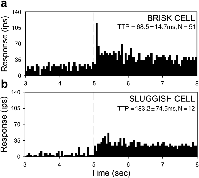
Like other mammals, rat RGCs could be divided into brisk and sluggish types based on their response to a small spot flashed over the RF center. Brisk cells responded to this stimulus with a crisp burst of activity 60–80 ms after spot onset, whereas sluggish cells responded with a slow smooth modulation of firing rate (Fig. 2). Brisk cells were recorded more frequently than sluggish cells (n = 175 vs. 21), presumably due to electrode bias for particular axons. They were also more uniform in behavior than sluggish cells, some of which had complex RF properties that took time to experimentally characterize. Brisk cells are thus the focus of the report.
Brisk and sluggish response dynamics. Response of an ON-center brisk RGC (a) and ON-center sluggish RGC (b) to a flashed spot matched in size to the RF center. Bin size of the PSTH is 50 ms. Dashed line indicates onset of standing contrast. TTP is the average (±s.d.) time-to-peak response, which was statistically different for the population of brisk- and sluggish-type cells (P < 0.01).

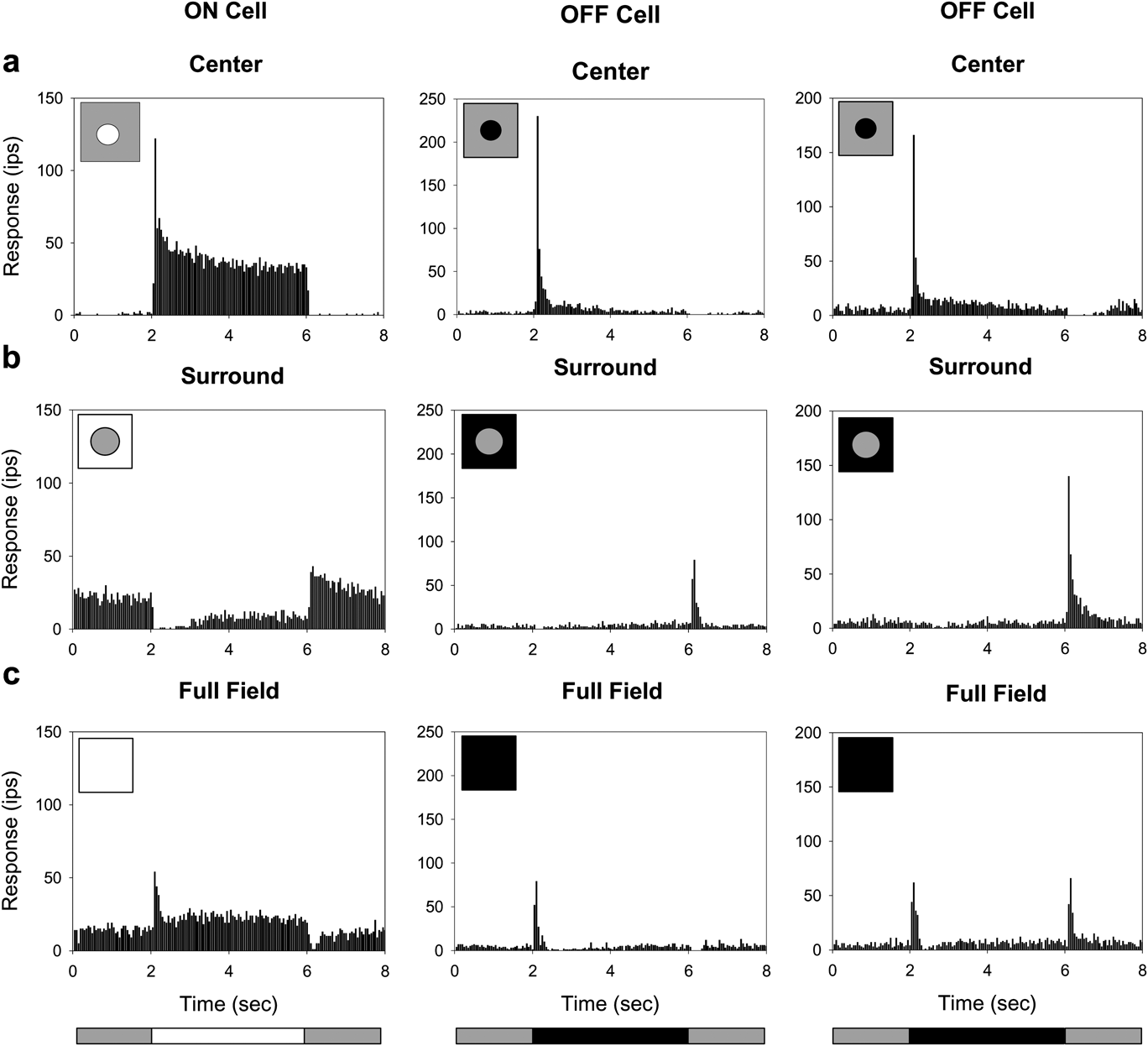
A common attribute of brisk cells was an antagonistic center-surround RF organization. The RF center was excited by a luminance increment for ON-type cells (n = 105) or a luminance decrement for OFF-type cells (n = 70) but not both (Fig. 3a), and the RF surround was excited by a luminance change in the opposite direction (Fig. 3b). ON- and OFF-center brisk cells differed in their response to full-field stimulation of both RF mechanisms. Like mouse RGCs (Sagdullaev & McCall, Reference Sagdullaev and McCall2005), the majority of OFF-center cells (n = 20 of 25 tested) produced an ON/OFF response to step variations in mean luminance, whereas all ON-center cells (n = 19) and the other OFF-center cells gave a conventional center-dominant response (Fig. 3c). The ON/OFF behavior implies that center and surround signals do not sum entirely linearly for a subpopulation of OFF-center brisk cells, or that an additional sign-altering mechanism operates in their RF surround.
Center-surround RF organization. Response of a typical ON-center and two types of OFF-center brisk RGC to a flashed: (a) spot matched to the RF center in size; (b) annulus with an inner diameter equal to the RF center; (c) full display field. Bottom illustration indicates the stimulus waveform. It repeated every 8 s and the average response to 15 presentations is shown.

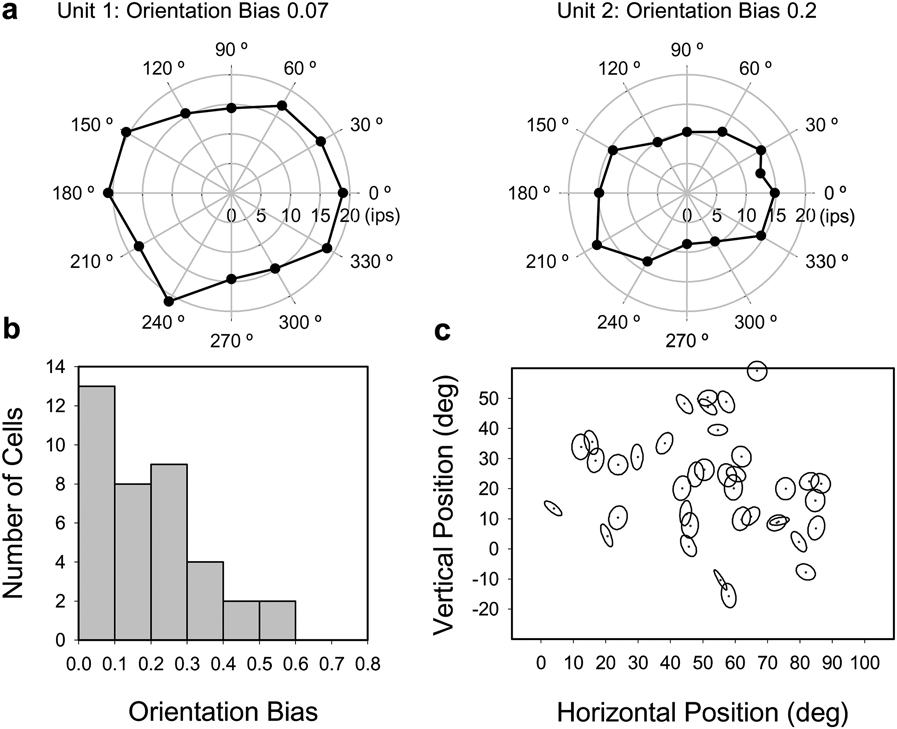
The spatial sensitivity profile of ganglion cell RFs is generally approximated as circular symmetric. Whether this approximation applies to rat was examined for a subset of brisk cells (n = 38) with drifting high spatial frequency gratings of various orientations (Fig. 4a). The degree of circular symmetry was quantified from the variation in F1 amplitude with orientation in terms of a bias index, which is 0 for a circle profile and 1 for a line profile. Orientation bias ranged up to 0.58 across the population, with a median of 0.19 (mean: 0.20 ± 0.14, Fig. 4b). Cells with a bias index greater than 0.3 had RF centers that were visibly oriented at a preferred angle. There was no apparent clustering of orientation biases across visual space (Fig. 4c), though a larger sample would be needed for a definitive statement. The measured bias distribution parallels that of cat RGCs, which was reported to range up to 0.46 with a median of 0.14 (Levick & Thibos, Reference Levick and Thibos1982). In subsequent experiments, grating patterns were optimally oriented for recorded cells.
RF center profile. (a) Center response profiles of two brisk RGCs collected with high spatial frequency drifting gratings of varying orientation. (b) Orientation bias histogram for 38 RGCs. Bin size is 0.1. (c) Distribution of orientation bias with respect to RF location in the visual field. Orientation bias is expressed in the panel by the degree of center ellipticity and preferred orientation by the angle of the major axis, which is uniform in length. RF location is represented on the vertical axis in degrees relative to eye level (0 deg). Data from both eyes are pooled on the horizontal axis with distance given in degrees with respect to the nose (0 deg).

Response threshold and linearity
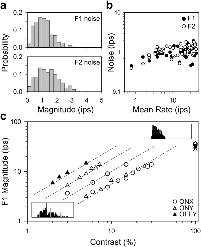
Most rat RGCs fire spikes at a maintained rate under steady illumination (Freeman et al., Reference Freeman, Heine and Passaglia2008). Because of the maintained discharge noise, a visual signal must exceed a certain level in order to produce a statistically detectable response. This level was specified for a subset of brisk cells (n = 45) by estimating the noise amplitude distribution at 2 and 4 Hz via Fourier analysis of long records of the maintained discharge. These frequency components were singled out because they correspond to the F1 and F2 response for stimuli used in this study. In every case, the F1 and F2 noise distributions overlapped extensively (Fig. 5a), and the maximum likelihood amplitude of both components was consistently 1–2 ips or less across the population of cells (Fig. 5b). Since the noise distributions would be inefficient to measure for every RGC, a visual response was considered physiologically significant if it exceeded a threshold level of 4 ips as an F1 or F2 amplitude larger than this has a low probability of chance occurrence (<1%).
Contrast response. (a) Probability distributions of F1 (empty) and F2 noise amplitudes (hatched) for a typical brisk RGC under photopic illumination. The maintained discharge was 22 ips and collected for 1 h. Bin size is 0.25 ips. (b) The root-mean-square of the F1 (black) and F2 (white) noise components for a population of 46 brisk cells with different maintained discharge rates. (c) F1 amplitude as a function of the contrast of a 2-Hz drifting sine wave grating of optimal spatial frequency for five brisk cells of varying mean rate (8, 41, 14, 5, and 27 ips from left to right) and responsiveness (peak F1 responsivity: 293, 176, 100, 61, and 54 ipsc, respectively). Insets show the PSTHs of one of these cells (responsivity: 61 ips, mean rate: 5 ips) for 5 and 100% contrast gratings. Lines indicate a linear contrast response function. For all panels, Fourier analysis was performed on 15-s segments of spike discharge with F1 and F2 amplitude measured for each segment at 2 and 4 Hz.

The linearity of brisk cell responses above the threshold level was assessed with full-field sine wave gratings of various contrast drifting at 2 Hz. Grating spatial frequency was optimized to stimulate the RF center maximally and the RF surround minimally. For a linear cell, the data would fall along a line of unity slope on log–log coordinates. Although F1 amplitude typically saturated for high contrast gratings, RGCs having widely different contrast sensitivity and mean firing rate all showed linear input–output behavior over a common response range (Fig. 5c). This range spanned from the noise floor to F1 amplitudes of at least 10 ips. In subsequent experiments, stimulus contrast was adjusted to produce responses in the linear range, so that RF measurements were not distorted by spike output nonlinearities.
Linear and nonlinear subtypes of brisk cell
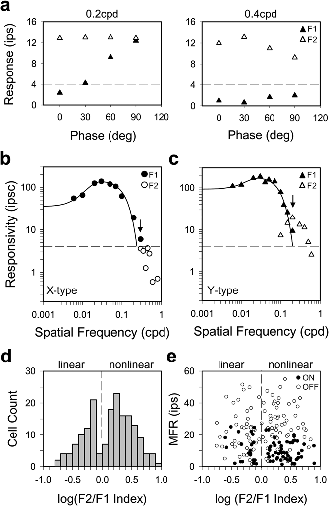
Brisk RGCs in cat can be divided into linear and nonlinear subtypes by performing a modified “null test” (Hochstein & Shapley, Reference Hochstein and Shapley1976), which uses contrast-reversing patterns to probe spatial summation within the RF. For linear (X-type) cells, response amplitude depends on the spatial phase of the pattern with respect to the RF center, and for a certain phase (the null phase), there is no response due to cancellation of signals from light and dark stimulus areas. Y-type cells differ from X-type cells by exhibiting an additional response component at twice the reversal frequency that is spatial phase invariant. The difference in behavior can be quantified by Fourier analysis, where F1 amplitude captures the phase-dependent (linear) component and F2 amplitude captures the phase-independent (nonlinear) component. Most of the recorded brisk cells (n = 110) exhibited Y-type behavior, which included spatial phase invariance (Fig. 6a) and F2 responses that peaked in amplitude at spatial frequencies beyond the cutoff of the F1 tuning curve (Fig. 6c). There were also many brisk cells, though (n = 65) for which a reversing grating did not elicit a significant frequency-doubled response (Fig. 6b). Since they exhibited X-type behavior, a spatial summation index was used to objectively sort rat brisk cells into linear and nonlinear subtypes. The index was defined as the ratio of F2 to F1 responsivity at the highest spatial frequency that yielded a suprathreshold F1 response (Fig. 6, arrows). If the F2 response peaked at a higher frequency, it was substituted into the calculation. Unlike cat (Hochstein & Shapley, Reference Hochstein and Shapley1976), the distribution of F2/F1 indices did not have a gap that cleanly delineates X and Y cells (Fig. 6d), as there were some ambiguous brisk cells with an index around one [7% with log (F2/F1) between ±0.1]. Nevertheless, the distribution was not unimodal according to the dip test of unimodality (Hartigan & Hartigan, Reference Hartigan and Hartigan1985; dip = 0.039, P < 0.05). This can be considered a conservative test because F2/F1 values are less meaningful for cells with little or no F2 response. If low index (i.e., linear) cells are lumped together, the bimodality of the data would be even greater. The linear–nonlinear dichotomy was not a byproduct of spike-rate rectification either (Mechler & Ringach, Reference Mechler and Ringach2002) since the criterion response amplitude of 5–10 ips was less than the mean spike rate of most cells and the mean rate was uncorrelated with nonlinearity index (Fig. 6e). RGCs with an F2/F1 index <1 are thereby referred to as brisk-linear (X-type) cells and those with an index >1 as brisk-nonlinear (Y-type) cells.
Linear and nonlinear subtypes of brisk cell. (a) F1 and F2 response amplitudes (black and white triangles) measured to sinusoidal contrast-reversing (2 Hz) gratings of different spatial phase (0–90 deg) from a brisk cell that shows nonlinear spatial summation. Spatial frequency is 0.2 cpd in the left panel, which falls on the high frequency limb of the F1 tuning curve in (c) and 0.4 cpd in the right panel, which exceeds the F1 resolution. (b) and (c) Spatial tuning curve of F1 responsivity to 2-Hz drifting gratings and F2 responsivity to 2-Hz reversing gratings for a linear (circles) and nonlinear (triangles) brisk cell. The arrow indicates the spatial frequency, at which the F2/F1 index would be calculated for these cells. The index is 0.6 for the linear (X-type) cell and 2.1 for the nonlinear (Y-type) cell. The solid lines are a DOG model fit of the F1 data, and the dashed line is the threshold response level as determined by Fig. 4. F2 amplitude was in the noise for the linear cell (b) and above response threshold for the nonlinear cell (c). (d) Histogram of nonlinearity indices for 175 brisk RGCs. (e) Maintained firing rate (MFR) of cells as a function of nonlinearity index. Dashed lines separate nonlinear cells, which show a marked F2 reversal response from linear cells that do not.

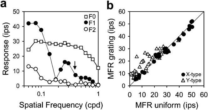
The behavior of brisk-linear and brisk-nonlinear cells differed in another related respect. Upon presentation of a full-field drifting grating, many Y-type cells increased their mean spike rate, in some cases, more than 20 ips above the maintained rate under steady uniform illumination (Fig. 7a). The mean rate increase was not caused by clipping of the modulated (F1) response as such a nonlinearity would also produce an F2 component, which was not observed except for low frequency gratings (<0.1 cpd). Moreover, the rate increase persisted out to ~1 cpd, which is well beyond the spatial acuity limit of the RF center (arrow). Drifting gratings had a measurable mean rate effect (>5 ips) on ~40% (n = 18 of 43) of Y-type cells and no (n = 27) X-type cells (Fig 7b). A similar X/Y disparity to this stimulus has been reported for cat brisk cells (Enroth-Cugell & Robson, Reference Enroth-Cugell and Robson1966; Passaglia et al., Reference Passaglia, Enroth-Cugell and Troy2001).
Many brisk-nonlinear cells respond to drifting gratings with an elevation in mean firing rate. (a) The first three Fourier components (F0, F1, and F2) of the response of a brisk-nonlinear cell to a 2-Hz drifting grating of varying spatial frequency. The maintained discharge (F0) for steady uniform illumination is 12 ips. (b) Summary data for 27 brisk-linear cells (circles) and 43 brisk-nonlinear cells (triangles). Mean firing rates (MFR) for grating stimuli were collected at spatial frequencies a little above the high frequency resolution of the fundamental response component. Cells on the diagonal line showed no grating-induced change in MFR.

It is important to note that our application of the terms “X-type” and “Y-type” to rat RGCs is strictly limited to brisk cells and their spatial summation properties. This is consistent with the original usage of the terms for classifying linear and nonlinear cells in the cat optic tract (Enroth-Cugell & Robson, Reference Enroth-Cugell and Robson1966; Hochstein & Shapley, Reference Hochstein and Shapley1976) since X and Y cells have brisk responses and are predominantly recorded with optic tract electrodes. The terms do not include sluggish cells and other “W-type” cells that are now known in cat to also show linear/nonlinear summation for reversing patterns or mean rate changes for drifting patterns, as their physiological behavior is distinct in several well documented aspects (Troy & Shou, Reference Troy and Shou2002). The terms should not be misinterpreted to include other reported differences between X and Y cells either, such as spatial or temporal resolution (Linsenmeier et al., Reference Linsenmeier, Frishman, Jakiela and Enroth-Cugell1982; Frishman et al., Reference Frishman, Freeman, Troy, Schweitzer-Tong and Enroth-Cugell1987). For one reason, some of those differences were not investigated here. For another, while brisk-linear and brisk-nonlinear cells may be the rat equivalent of cat X and Y cells, their RF properties are not homologous with respect to center size as described below.
Spatial frequency response of brisk cells
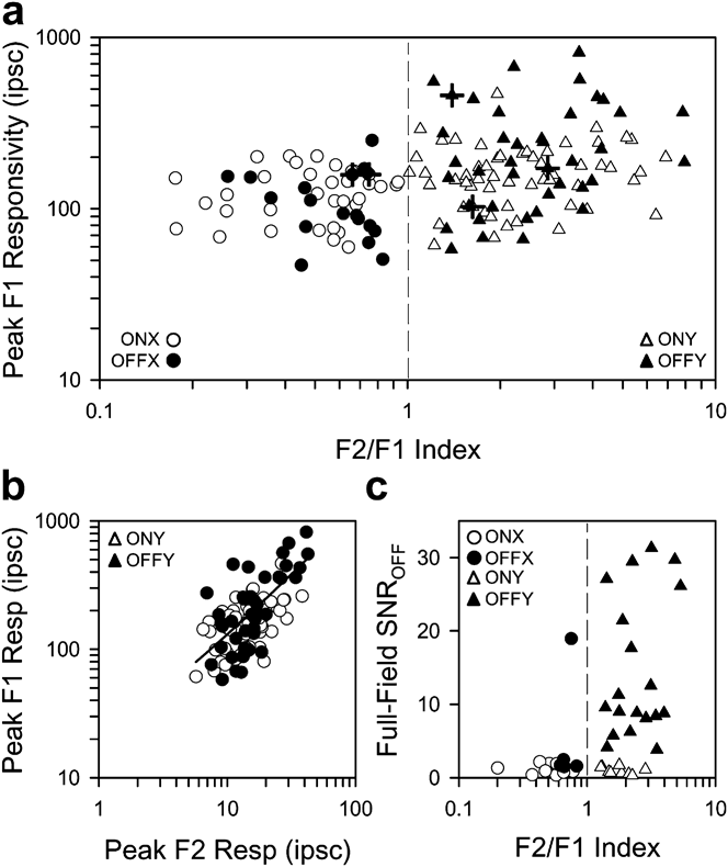
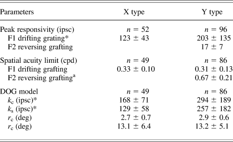
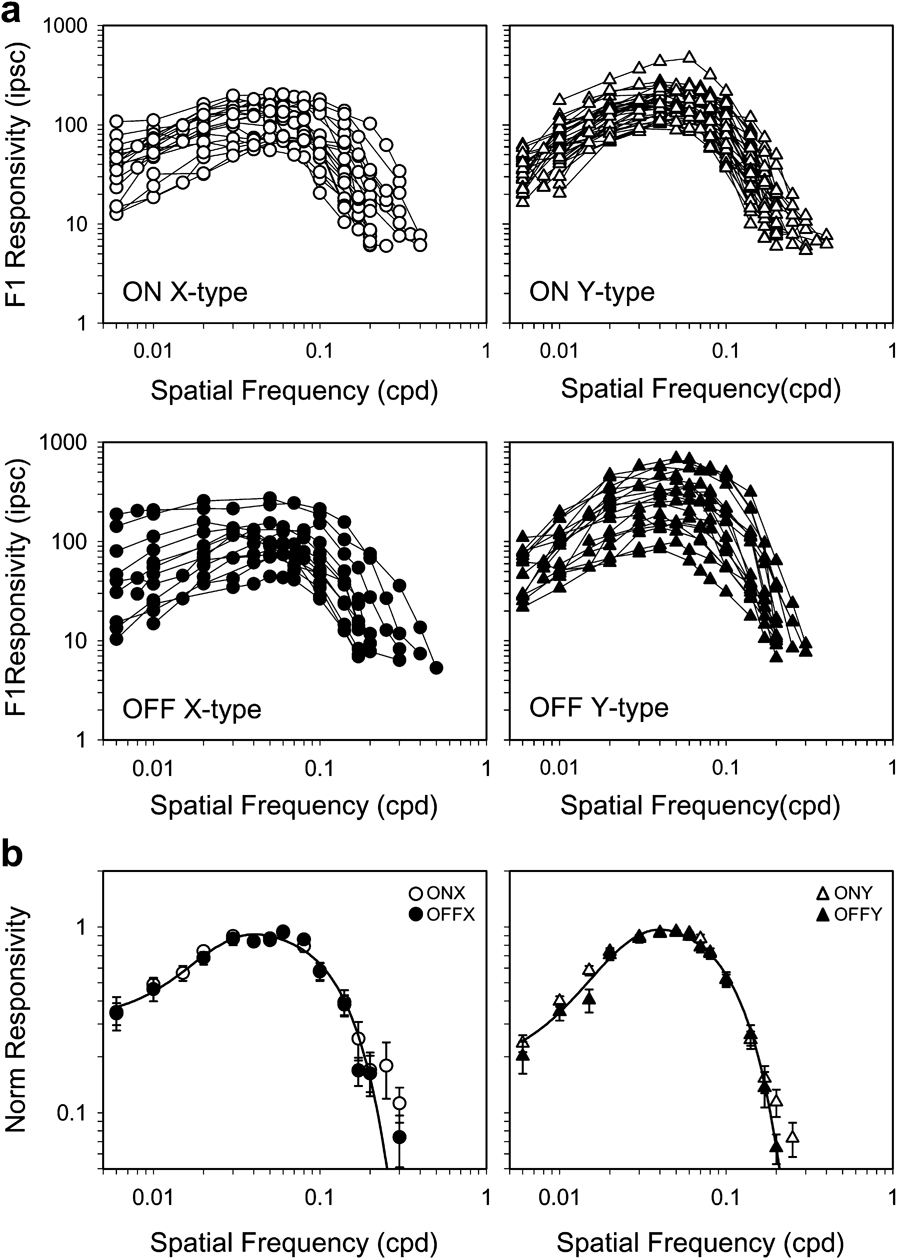
There was considerable variability in contrast sensitivity across the population of brisk cells. The peak F1 responsivity ranged from 50 to 250 ipsc for X-type cells and 60 to 820 ipsc for Y-type cells (Fig. 8a), even though retinal illuminance was held constant. The broad range cannot be attributed solely to experimental variation, as responsivity could vary markedly among cells in the same animal (crosshairs). It was greater for Y-type cells (ON: 167 ± 71 ipsc, n = 56; OFF: 252 ± 181 ipsc, n = 40) than X-type cells (ON: 127 ± 42 ipsc, n = 35; OFF: 115 ± 52 ipsc, n = 17), with OFF-center Y-type cells showing the greatest responsivity of all (Tukey–Kramer test, P < 0.05). F1 responsivity also covaried in Y-type cells with F2 responsivity (Fig. 8b, Rsq = 0.49). Linear regression of the data gave a slope of 12, meaning that the nonlinear RF component is about a log unit less responsive than the linear RF center (Table 1). This nonlinear mechanism might also be involved in the ON–OFF response of OFF-center brisk cells to step changes in full-field illumination (see Fig. 3c) because it was associated primarily with Y-type cells (Fig. 8c).
Response properties of brisk-linear and brisk-nonlinear cells. (a) Peak F1 responsivity of ON- and OFF-center brisk cells (white and black symbols) as a function of F2/F1 index. X-type cells (circles) are defined by F2/F1 indices <1 and Y-type cells (triangles) by indices >1 (dashed line). Crosshairs mark data points from the same animal. (b) Peak F1 responsivity of ON- and OFF-center brisk-nonlinear cells as a function of peak F2 responsivity. The line is a linear regression of the data (intercept = 12.4 ipsc, slope = 11.8, R 2 = 0.49). F1 and F2 responsivities were measured with drifting and reversing gratings. (c) OFF response to step changes in full-field illumination as a function of F2/F1 index. Response magnitude is expressed in terms of signal-to-noise ratio (SNR), which was defined as the peak rate in the first 1 s of the OFF response divided by the average rate over the following 3 s.

Summary of spatial tuning properties

Values are mean ± s.d. A significant difference (P < 0.05) between X- and Y-type cells is denoted by asterisks next to the parameter. F1 and F2 acuity values correspond to the spatial frequency at which the DOG model fit and measured response respectively fell below the noise threshold.
a n = 22.
In general, the spatial frequency response of all brisk cells showed characteristics of a band-pass filter with peak F1 responsivity for 2-Hz drifting gratings at around 0.05 cpd (Fig. 9a). Such filtering properties are indicative of a linear center-surround RF organization. The spatial acuity limit, defined as the frequency at which the F1 response fell below the noise level, was statistically indistinguishable for X- and Y-type cells, averaging around 0.32 cpd (Table 1). For each brisk cell type, there were some tuning curves that did not present much low frequency response attenuation and better resembled a low-pass filter. This could reflect the absence of a surround mechanism, but it can also be attributed to the large size of rat RFs and the limited area of the visual display, as the grating pattern might stimulate a fraction of the RF surround of cells near the display margins. In view of the variability in RGC responsiveness, spatial tuning curves were normalized by peak responsivity and averaged for each brisk cell type (Fig. 9b). The normalized curves describe the average spatial RF profile independent of cell sensitivity. Like the spatial acuity limit, the frequency of half-maximal responsivity was nearly equal for X-type (0.10 ± 0.02 cpd, n = 49) and Y-type (0.12 ± 0.04 cpd, n = 86) cells, though the small difference was statistically significant in this case (Student’s t-test, P < 0.05). The similar RF center size of brisk-linear and brisk-nonlinear cells is unlike that of cat X and Y cells. It cannot be explained by experimental factors like eye defocus because i) the measured cutoff frequency changed little when auxillary lenses between ±6 diopters were inserted into the visual path (data not shown), in agreement with prior findings (Artal et al., Reference Artal, Herreros de Tejada, Redó and Green1998), and ii) F0/F2 responses were measured for drifting/reversing gratings above the F1 cutoff frequency (Figs. 6c and 7a). The F2 spatial acuity limit averaged 0.67 cpd for highly nonlinear Y-type cells (F2/F1 index >2) and reached up to 1.2 cpd in some cases (Table 1).
Spatial frequency response of brisk cell subtypes. (a) Spatial tuning curves of all ON- and OFF-center (white and black symbols) brisk-linear (circles) and brisk-nonlinear (triangles) cells for 2-Hz full-field drifting gratings. (b) Average tuning curve after normalizing the data in (a) by the peak responsivity of each cell. Each point is the average of at least four cell measurements. Error bars give s.d. Solid line in (b) is a DOG model fit of the X-type and Y-type datasets (k c = 1.13 and 1.01, k s = 0.95 and 0.70, r c = 2.7 and 2.2 deg, and r s = 14.4 and 14.7 deg).

RF center and surround measurements
To quantify the size and strength of RF center and surround mechanisms, the spatial sensitivity profile was modeled by a DOG function that took into account the RF location on the visual display to mitigate edge effects on surround estimates. Only brisk cells with weak orientation bias were considered (<0.3) because the model assumes the sensitivity profile is circular symmetric. The DOG function was simultaneously fit to two separate measures of the spatial sensitivity profile: one was the frequency response (Fig. 10a) and the other was the response to sinusoidally modulated spots of varying radii (Fig. 10b). Spot response data served as an additional constraint on surround size. The model gave a reasonable fit to both RF measurements, and summary parameter values are provided in Table 1. Estimates of RF center and surround strength were both greater for Y-type cells than for X-type cells, with the ratio of center-to-surround strength averaging 1.27 ± 0.30 for all brisk cells (Fig. 10c, left). Estimates of RF center and surround radii, on the other hand, showed no significant differences between ON- or OFF-center X- and Y-type cells (Fig. 10c, right). Across the population center, radius ranged from 1.1 to 4.7 deg about a median of 2.8 deg, while surround radius ranged from 4.4 to 29.1 deg about a median of 12.3 deg. Any correlation between center-surround sizes was extremely weak (Rsq = 0.08). These measurements are consistent with prior studies of rat RGCs, which report center diameters from 3 to 15 deg with a mean of 7.5 deg (Brown & Rojas, Reference Brown and Rojas1965; Partridge & Brown, Reference Partridge and Brown1970). In those studies, the diameter was estimated from the spot size that produced the maximum response (Fig. 10a). This diameter corresponds to the distance between zero crossings of spatial sensitivity profiles computed by the DOG model, which averaged 7.3 ± 2.4 deg for our data.
RF center and surround measurements. (a) and (b) Responsivity of a brisk cell in space and spatial frequency measured with a spot matched in size to the RF center (a) and drifting gratings (b). Both stimuli were sinusoidally modulated at 2 Hz, and both datasets were simultaneously fit by a DOG model of the RF sensitivity profile. (c) Average center (light bars) and surround (dark bars) strengths and radii of brisk-linear (ONX/OFFX) and brisk-nonlinear (ONY/OFFY) cells. Error bars give s.d. Asterisks indicate pairs of datasets, for which RF parameters were significantly different (Tukey–Kramer test, P < 0.05).

The spatial properties of brisk cells were further examined with respect to RF location in visual space. Measurements from both eyes were combined using the nose as a reference point (horizontal location: 0 deg) in order to more fully map the rat’s visual field. The RFs of recorded cells were spread throughout much of the space accessible to our stimulus display system (Fig. 11a), including frontal regions that would provide for some binocular vision (Reese & Cowey, Reference Reese and Cowey1986; Grieve, Reference Grieve2005). There was, however, a curious paucity of cells with RFs in the ventronasal region that is swept by whisker movements. Overall, the distribution of RF locations was not uniform (Fig. 11b), with nearly half of recorded cells viewing a region 15–55 deg above eye level and 30–70 deg lateral to the nose. The nonuniform representation of visual space suggests that RF size might covary in a similar manner. However, center and surround radii were both independent of horizontal and vertical location (Fig. 11c and 11d). Moreover, the scatter in surround radius estimates was fairly consistent across vertical space, suggesting that the variability is physiological in origin. If the scatter were due to edge-effect errors, it should decrease toward the middle of the display (∼25 deg vertical) where the surround would be activated more fully.
RF map of visual space. (a) Distribution of the center radii across the rat’s visual field. Data from both eyes were combined as in Fig. 4. Symbols are scaled to center radii, with thick lines corresponding to X-type cells and thin lines to Y-type cells. (b) Distribution of cell counts as a function of horizontal (top) and vertical (side) location in space. (c)and (d) Center and surround radii of brisk cell subtypes as a function of horizontal (top) and vertical location.

Spatial response properties of W-type cells
In the course of study, a small heterogeneous collection of RGCs was encountered with physiological characteristics distinct from those of brisk cells, in that, their spot responses were generally sluggish (Fig. 2) and their RFs were often large and hard to pinpoint. Spatial frequency responses could be measured for several cells (n = 14) and showed a low-pass characteristic for 2-Hz drifting gratings (Fig. 12a). This could mean they lacked a surround mechanism, except the high frequency cutoff was 5–10 fold less than that of a typical brisk cell. Given the large center size (r c = 13.1 ± 7.9 deg), a surround could have existed beyond the limits of the visual display. In addition to broad spatial tuning, the center responsivity was fairly low (K c = 43.1 ± 29.2 ipsc). The combination of spatial and temporal features readily distinguished sluggish cells from brisk cells (Fig. 12b). This was validated quantitatively by k-means clustering, which formed the same cell groupings when parsing the data in two (ellipses), and by the distribution of center strength per unit area (Fig. 12c), which had more than one mode (dip = 0.052, P< 0.05). Some RGCs did not present a classic center-surround RF structure. One of these W-type cells (n = 2) gave a phasic ON–OFF response to stimulation throughout its RF (local-edge-detector cell; Cleland & Levick, Reference Cleland and Levick1974), as demonstrated in rat recently (Girman & Lund, Reference Girman and Lund2010). Another (n = 2) did not modulate its firing rate to drifting gratings but instead lowered its maintained discharge (suppressed-by-contrast cell; Rodieck, Reference Rodieck1967). The mean spike rate was suppressed for grating frequencies up to 0.7 cpd (Fig. 12b), similar to the F0 (Fig. 7a) and F2 (Table 1) responses of Y-type cells, as observed in cat (Troy et al., Reference Troy, Einstein, Schuurmans, Robson and Enroth-Cugell1989). An unusual W-type cell (n = 3) was also identified that fired a single strong slightly-delayed burst of spikes at the onset of a spot centered on the RF, suggestive of a linear center mechanism, but fired at both stimulus onset and offset when surrounding area was illuminated (Fig. 12c), irrespective of annulus area for the most part. The ON–OFF behavior of the surround mechanism is different from that of OFF-center brisk cells, which respond only at annulus offset (Fig. 3b).
Spatial RF properties of sluggish cells. (a) Spatial tuning curves of 10 ON-center and 4 OFF-center sluggish cells (white and black squares) to 2-Hz full-field drifting gratings. The line is the average tuning curve of brisk cells from Fig. 9b scaled to 100 for purpose of comparison. (b) Center strength and radius estimates from DOG model fits of the spatial frequency response of sluggish cells (squares) as compared to brisk X-type and Y-type cells (circles and triangles). The brisk and sluggish data form clusters that can be objectively identified by k-means clustering the data in two groups (ellipses). (c) Distribution of RF center strength per unit area ( ) for all rat RGCs. Two modes are evident, corresponding to sluggish and brisk cell populations. (d) A suppressed-by-contrast W-type cell, which ceased firing when presented with drifting gratings below a certain spatial frequency (~0.4 cpd). (e) A novel W-type cell with linear RF center and an ON–OFF surround. PSTHs (bin size: 64 ms) were collected by alternating the stimulus (ON period) with a uniform gray screen (OFF period). The stimulus was a 30-deg spot over the RF center (left panel) or an annulus with a 30-deg inner diameter and 90-deg outer diameter over the RF surround (right panel).

Discussion
The spatial RF properties of rat RGCs were quantitatively described using grating, spot, and annulus stimuli in conjunction with a DOG model of center and surround mechanisms. ON- and OFF-center brisk and sluggish cell types were identified based on spot response polarity and dynamics. Brisk-type cells were also distinguished from sluggish-type cells by their heightened responsivity and increased spatial resolution. Brisk cells were further subdivided into linear and nonlinear types based on their spatial summation properties, which resembled those of cat X and Y cells. These properties included frequency-doubled responses to reversing gratings and mean rate changes to drifting gratings. Like mouse but not other mammals, the majority of OFF-center brisk cells contained an additional sign-inverting mechanism in the RF surround that resulted in ON–OFF responses to step changes in full-field illumination. This mechanism was expressed by Y-type and not X-type cells in all but one case. On the whole, brisk-nonlinear cells were more responsive than brisk-linear cells. Their spatial acuity, on the other hand, was virtually identical. The homogeneity of RF center size among X- and Y-type cells in rat is a peculiar finding that has broad relevance for the roles these types of mammalian RGC are thought to play in spatial information processing.
RF properties in relation to other species
Rat RGCs exhibit an antagonistic center-surround RF that is slightly elliptical in shape. The ellipticity imparts brisk cells with a measurable sensitivity to stimulus orientation, which is comparable to that of cat RGCs and somewhat stronger than that of primate RGCs (Hammond, Reference Hammond1974; Levick & Thibos, Reference Levick and Thibos1982; Passaglia et al., Reference Passaglia, Troy, Ruttiger and Lee2002). No stimulus orientation appeared overly represented by the brisk cell population, presumably because the rat lacks a central high-acuity field like cat and primate which show a bias for radial and tangential RF orientations. Elliptical RFs of no particular orientation can also be seen in an in vitro study of rat RGCs (Anishchenko et al., Reference Anishchenko, Greschner, Elstrott, Sher, Litke, Feller and Chichilnisky2010), suggesting that it reflects the elongated morphology of RGC dendritic trees. Indeed, our physiological measurements of orientation sensitivity agree well with anatomical estimates for rat (mean bias index: 0.19, Schall et al., Reference Schall, Perry and Leventhal1987). The elliptical RF shape is passed onto LGN cells (Sumitomo et al., Reference Sumitomo, Sugitani, Fukuda and Iwama1979; Grubb & Thompson, Reference Grubb and Thompson2003; van Hooser et al., Reference van Hooser, Heimel and Nelson2003) and may help to build orientation selectivity in the rat visual cortex (Girman et al., Reference Girman, Sauve and Lund1999). It may also factor into the complex orientation-specific center-surround interactions recently reported in rat retina (Girman & Lund, Reference Girman and Lund2010).
In cat and primate, RFs are smallest near the center of the retina and increase toward the periphery due to an eccentricity-dependent expansion of RGC dendritic trees (Peichl & Wassle, Reference Peichl and Wassle1979; Lee et al., Reference Lee, Kremers and Yeh1998). Our data offer no support for a peripheral expansion of RFs in rat, though they do suggest a nonuniform sampling of the visual field (Figs. 4 and 11). This is also consistent with anatomical studies, which report no systematic variation of dendritic tree size with retinal eccentricity except perhaps for one morphological cell type (Huxlin & Goodchild, Reference Huxlin and Goodchild1997; Sun et al., Reference Sun, Li and He2002). Rats are not unique in this regard either as RF and dendritic tree sizes are independent of retinal location in mouse as well (Lin et al., Reference Lin, Wang and Masland2004; Sagdullaev & McCall, Reference Sagdullaev and McCall2005). In cat, the smallest RFs belong to X cells, and near the area centralis, their RF center is comparable in size to the nonlinear subunits of the frequency-doubling mechanism of Y cells, from which it was inferred that the same retinal elements probably provide input to both mechanisms (Enroth-Cugell & Freeman, Reference Enroth-Cugell and Freeman1987). These elements are thought to be bipolar cells (Demb et al., Reference Demb, Zaghloul, Haarsma and Sterling2001). Since the subunits are several fold smaller than the RF center of both brisk cell types in rat (Table 1), it would appear that there is extensive pooling of bipolar signals in the inner retina by RGCs throughout the rodent retina.
To date, the physiological properties of rat RGCs have not been systematically examined for possible differences beyond center polarity (ON or OFF). One reason for this might be that brisk cells are most often recorded electrophysiologically, and our results indicate that they all have similar RF size. A difference in temporal properties might be expected from work on other mammals (Cleland et al., Reference Cleland, Dubin and Levick1971; Cleland & Levick, Reference Cleland and Levick1974), and indeed, brisk and sluggish cell types were found. Sustained and transient subtypes of brisk cell have also been described recently in rat (Girman & Lund, Reference Girman and Lund2010). Response dynamics were not emphasized here, as sustained/transient distinctions can be obscured by the state of adaptation, which varies with RF center area (Jakiela & Enroth-Cugell, Reference Jakiela and Enroth-Cugell1976). When brisk cells were tested for spatial summation X- and Y-types were identified, consistent with a study that applied the test to a handful of rat LGN cells (Lennie & Perry, Reference Lennie and Perry1981). That study also noted a similarity of RF size among the two cell types, so we considered whether brisk cells might express a continuum of spatial summation properties with some more nonlinear than others and therefore constitute a single physiological group, as posited for visual cortical cells (Mechler & Ringach, Reference Mechler and Ringach2002). However, several aspects of our data argue against the idea. First, although rat brisk cells exhibited a broad range of F2/F1 indices that made some cells difficult to classify, the distribution of indices was distinctly bimodal (Fig. 6d) and the bimodality could not be explained by spike-rate rectification of modulated responses due to the lack of a maintained discharge (Fig. 6e). Second, several low index (F2/F1 < 0.8) cells had an F1 responsivity over 100 ips (Fig. 8a) yet lacked an F2 response altogether, meaning they were not Y-type cells that looked linear by virtue of poor contrast sensitivity. Third, none of the low index cells produced a modulated response to a contrast-reversing edge centered on the RF (data not shown). Fourth, drifting gratings affected the mean firing rate of high index cells only (Fig. 7b). And last, ON–OFF responses to step illumination changes were associated primarily with high index cells and not low index cells (Fig. 8c). Such X/Y dichotomies in behavior have been observed in other in vivo rodent studies (McCourt & Jacobs, Reference McCourt and Jacobs1984; van Hooser et al., Reference van Hooser, Heimel and Nelson2003). An in vitro mouse study, however, found that they did not reach a level of significance for cell classification (Carcieri et al., Reference Carcieri, Jacobs and Nirenberg2003). That study identified an abundance of nonlinear cells in comparison to linear cells, so perhaps this reflects an oversampling of Y-type RGCs by intraretinal arrays with homogeneous electrode properties or a “linearizing” effect of anesthesia on spatial summation properties, as an in vivo mouse study reported mostly X-type cells in the LGN (Grubb & Thompson, Reference Grubb and Thompson2003).
The non-brisk RGCs that were encountered bore strong resemblance to assorted W-type cells in other mammals. For example, sluggish cells had large RFs, center-surround organization, and relatively low visual responsivity (Cleland & Levick, Reference Cleland and Levick1974; Stone & Fukuda, Reference Stone and Fukuda1974; Caldwell & Daw, Reference Caldwell and Daw1978; Rowe & Cox, Reference Rowe and Cox1993; Merwine et al., Reference Merwine, Amthor and Grzywacz1995; Troy et al., Reference Troy, Schweitzer-Tong and Enroth-Cugell1995), while other cells gave only ON–OFF responses like local-edge-detector cells or mean rate changes like suppressed-by-contrast cells (Levick, Reference Levick1967; Rodieck, Reference Rodieck1967; van Dongen et al., Reference van Dongen, ter Laak, Thijssen and Vendrik1976; Troy et al., Reference Troy, Einstein, Schuurmans, Robson and Enroth-Cugell1989; Tailby et al., Reference Tailby, Solomon, Dhruv, Majaj, Sokol and Lennie2007). One cell type (ON–OFF surround) was fairly novel in terms of its response to flashed spots and annuli. Only one study to our knowledge mentions RGCs with a pure center and mixed surround (Winters et al., Reference Winters, Hickey and Pollack1973).
RF properties in relation to rat visual acuity
Behavioral estimates consistently place the limit of rat spatial acuity between 0.5–1.0 cpd (Lashley, Reference Lashley1938; Wiesenfeld & Branchek, Reference Wiesenfeld and Branchek1976; Dean, Reference Dean1978; Cowey et al., Reference Cowey, Henken and Perry1982; Linden et al., Reference Linden, Cowey and Perry1983). This limit falls within the physiological range for visually evoked cortical potentials and cortical spike recordings (Silveira et al., Reference Silveira, Heywood and Cowey1987; Girman et al., Reference Girman, Sauve and Lund1999) but is noticeably higher than that of RGCs. While we cannot exclude the possibility that a high-acuity population of brisk cell was missed by our optic tract electrode, the measured cutoff frequency of ~0.2 cpd is consistent with prior studies of subcortical neurons in rat. Powers and Green (Reference Powers and Green1978), for example, published spatial tuning curves for unclassified RGCs that peaked between 0.02 and 0.07 cpd and dropped into noise by 0.4 cpd. Prévost et al. (Reference Prévost, Lepore and Guillemot2007) reported cutoff frequencies in the same range for superior colliculus cells. And Lennie and Perry (Reference Lennie and Perry1981) noted no difference in spatial resolution of X- and Y-type LGN cells, with both rolling off around 0.1 cpd. There is one study, however, that reports a bimodal distribution of spatial acuity with one mode centered near 0.8 cpd (Friedman & Green, Reference Friedman and Green1982), suggesting that a high-acuity population of RGCs may exist. It is unclear though whether the high-acuity cells are actually different from those described here and elsewhere because that study used auditory cues to specify the finest resolvable grating, whereas our estimates are based on the frequency at which F1 spatial tuning curves fall below noise level. If nonlinear response components are considered, the acuity limits become comparable since Y-type cells can provide cues out to ~1 cpd (Fig. 7, Table 1). The disparity in spatial acuity of RGCs and animal behavior could also be explained by information available to the rat from other neural channels besides brisk cells. For example, local-edge-detector cells have the smallest RFs in rabbit and were implicated in the detection of fine spatial gratings (Zeck et al., Reference Zeck, Xiao and Masland2005; van Wyk et al., Reference van Wyk, Taylor and Vaney2006). The rat could also use other stimulus features to solve the detection task, such as edge effects that result when gratings are viewed through an aperture. The edges of a display can produce a flicker percept in humans even for patterns that are not resolvable, which may lead to overestimation of spatial acuity (Barlow, Reference Barlow1965; Campbell et al., Reference Campbell, Carpenter and Levinson1969). We could produce such effects in rat RGCs and extend F1 spatial tuning curves beyond 1 cpd by positioning the RF center on a display edge and drifting gratings parallel to the edge (data not shown).
Functional role of X- and Y-type cells in rat
The marked difference in RF center diameter of X and Y cells in cat, together with their distinct axon conduction velocity, temporal resolution, and central projection pattern, has been interpreted to mean that X cells subserve spatial vision and Y cells motion vision (Shapley & Perry, Reference Shapley and Perry1986). This interpretation is less compelling for rat since there is no obvious advantage for its visual system to relegate spatial information to one of these channels when both integrate over similar areas. Apparently, linear/nonlinear summation has a role in retinal signaling that is distinct from summation area. We also point out that the homogeneity of RF center diameter of X and Y type RGCs is a trait common to several other prey species, including mouse, rabbit, and gray squirrel (Vaney et al., Reference Vaney, Levick and Thibos1981; Stone & Pinto, Reference Stone and Pinto1993; van Hooser et al., Reference van Hooser, Heimel and Nelson2003). It could be related to the small size of these animals since the strong curvature of small eyes does not provide for fine quality images (Artal et al., Reference Artal, Herreros de Tejada, Redó and Green1998). Perhaps, it reflects the opponent ecological niches of predator and prey species. Prey animals like rat rely heavily on olfaction and whisker movements, and vision for them may serve more like an alert system designed to detect any large potentially threatening object as opposed to discriminate targets from their surroundings.
Acknowledgments
This work was supported by NIH R01 EY016849 and a Smith Family New Investigator Award. W.F.H. was partially supported by the NIH Training Grant T32 GM008541. We thank Dan Freeman and Gilberto Graña for technical assistance.