



1. Introduction
Bedload transport is a special kind of sediment transport in which typically coarse sedimentary grains roll, slide and hop along the surface in response to the shearing of a loose granular bed by a flow of liquid. It plays a vital role in shaping the environments of Earth and other planetary bodies (Poggiali et al. Reference Pähtz, Chen, Zhu, Tholen and He2016) by promoting the formation and growth of geological features of various scales, including ripples and dunes (Charru et al. Reference Charru, Andreotti and Claudin2013; Durán Vinent et al. Reference Durán Vinent, Andreotti, Claudin and Winter2019), deltas and fans (Baker et al. Reference Baker, Hamilton, Burr, Gulick, Komatsu, Luo, Rice and Rodriguez2015), and laminations and cross-bedding (Schieber Reference Schieber2016; Shchepetkina et al. Reference Shchepetkina, Gingras, Mángano and Buatois2019). A key problem hampering our understanding of bedload-induced landscape evolution is the notoriously large noise commonly associated with measurements of the bedload flux, often exceeding an order of magnitude (Recking Reference Recking2010; Ancey & Recking Reference Ancey and Recking2023). It partially originates from huge non-Gaussian flux fluctuations over large time scales, which even occur under steady flow conditions in the laboratory due to continuous topographic change (Dhont & Ancey Reference Dhont and Ancey2018). However, also when restricted to steady flows over flat beds at short time scales, reported bedload fluxes can still substantially differ between laboratory studies for largely self-similar conditions, for both weak and intense transport-driving flows (Ancey & Recking Reference Ancey and Recking2023), and it has been unclear whether such differences arise due to physical or experimental reasons. On the one hand, physical reasons may come into play because dissimilarities in grain size and shape distributions are not accounted for by commonly used similarity parameters. On the other hand, study-to-study variability of the geometry of laboratory facilities is a potential culprit on the experimental side, especially in view of the associated large random and systematic uncertainties in the experimental determination of the transport-driving bed shear stress
 $\tau _b$
(Yager et al. Reference Yager, Venditti, Smith and Schmeeckle2018). Focusing here on rectangular open channels, since they are geometrically similar to natural streams, the ratio
 $b/h$
between the channel width
 $b$
and flow depth
 $h $
is a crucial parameter in this regard. Ideally, one would want
 $b/h$
to be as large as possible to most closely resemble bedload transport in nature. However, in experimental reality,
 $b/h$
is often of order unity, substantially weakening the shearing of the bed due to frictional losses at the sidewalls, causing the flow to be non-uniform in the cross-channel direction (Guo Reference Guo2015). Another important parameter is the ratio between
 $h$
and the grain diameter
 $d$
. For shallow channel flows where
 $h/d$
is close to unity, the method by which the bed surface elevation, and thus the flow depth
 $h$
above it, is identified can have a large effect on the value of
 $\tau _b$
.
To illustrate that channel geometry effects often are not appropriately accounted for, we choose two laboratory studies measuring bedload flux over a flat bed: Ni & Capart (Reference Ni and Capart2018), who conducted their experiments in a wide but shallow channel (
 $h/d\sim 2{-}6$
), and Deal et al. (Reference Deal, Venditti, Benavides, Bradley, Zhang, Kamrin and Perron2023), who used a very narrow but deep channel (
 $b/h\approx 0.1$
). Since the grains in both studies were spherical and relatively uniformly sized, one expects the same quantitative behaviour of the non-dimensionalised bedload flux
 $Q_\ast$
as a function of the non-dimensionalised bed shear stress or Shields number
 $\varTheta$
(Ancey Reference Ancey2020). However, when using these studies’ reported values for
 $\varTheta$
and
 $Q_\ast$
, based on their own definitions and methods to determine
 $\tau _b$
, both datasets disagree with each other by a staggering factor of approximately
 $6$
for
 $\varTheta \approx 0.2$
(figure 1). This indicates that at least one of them was inappropriately correcting for channel geometry effects, showcasing the need for a universal channel geometry correction method.
Bedload flux measurements for spherical grains by Ni & Capart (Reference Ni and Capart2018) and Deal et al. (Reference Deal, Venditti, Benavides, Bradley, Zhang, Kamrin and Perron2023). The Shields number
 $\varTheta$
and non-dimensionalised bedload flux
 $Q_\ast$
are defined and determined as described in these studies. For
 $\varTheta \approx 0.2$
, the values of
 $Q_\ast$
disagree with each other by a factor of approximately
 $6$
.

This study addresses two of the mentioned potential reasons for the study-to-study variability of laboratory bedload flux measurements: grain shape and channel geometry effects. We compile existing and new data of turbulent bedload transport along flat beds (no bedforms) of shape-controlled and (relatively) uniformly sized grains, obtained from experiments and grain-resolved (i.e. directly resolving fluid–particle interactions) and grain-unresolved numerical simulations based on various computational fluid dynamics/discrete element method (CFD-DEM) techniques, across channel flow widths and heights, grain shapes, bed slopes and flow strengths. In § 2, we reconcile channel geometry effects in these data through a universal sidewall correction, based on linking Reynolds stress to bulk flow properties via an extension of Kolmogorov’s theory of turbulence (Gioia & Bombardelli Reference Gioia and Bombardelli2002; Gioia & Chakraborty Reference Gioia and Chakraborty2006), and a granular-physics-based definition to precisely determine the bed surface elevation (Pähtz & Durán Reference Pähtz and Durán2018b
). This channel geometry correction method is validated, among others, through a collapse of experimental and grain-resolved numerical bedload flux data for spherical grains on a unique behaviour, whereas classical methods (Einstein Reference Einstein1942; Johnson Reference Johnson1942; Guo Reference Guo2015, Reference Guo2017) yield very large scatter. Furthermore, in § 3, we generalise an existing physical bedload flux model (Pähtz & Durán Reference Pähtz, Liu, Xia, Hu, He and Tholen2020) to account for grain-shape effects. It agrees with the entire channel-geometry-corrected data compilation within a factor
 $1.3$
. The results are then discussed in § 4, and conclusions are drawn in § 5.
2. Universal channel geometry correction method
In this section, we derive and validate a universal channel geometry correction method to determine the transport-driving bed shear stress
 $\tau _b$
for open channels with hydraulically rough sediment beds and hydraulically smooth sidewalls. We begin with the definition of
 $\tau _b$
(§ 2.1), and derive from it, partially using known results, an expression that contains the flow depth
 $h$
and the effective mixture sidewall shear stress
 $\tau _w$
as unknowns. We then propose to determine
 $h$
from an existing granular-physics-based definition of the bed surface elevation (§ 2.2), and derive an expression for
 $\tau _w/\tau _b$
from an extension of Kolmogorov’s theory of turbulence (§ 2.3). In § 2.4, the resulting channel geometry correction method is tested against a data compilation of turbulent bedload transport of spherical grains and other data.
2.1. Definition of bed shear stress
For turbulent bedload transport in open channels with hydraulically rough sediment beds, there is a limited region in the clear-water flow above the bedload layer where the streamwise (
 $x$
) fluid velocity profile
 $u_x(z)$
approximately obeys the logarithmic law of the wall (Kidanemariam Reference Kidanemariam2016; Jain et al. Reference Jain, Tschisgale and Fröhlich2021; Deal et al. Reference Deal, Venditti, Benavides, Bradley, Zhang, Kamrin and Perron2023):
 \begin{equation} u_x\approx \frac {u_\tau }{\kappa }\ln \frac {z+z_o}{z_o}, \end{equation}
where
 $\kappa =0.41$
is the von Kármán constant,
 $z$
is the bed-normal coordinate, with
 $z=0$
the bed surface elevation,
 $z_o$
is the hydrodynamic roughness, which depends on both grain size and bedload flux (Durán et al. Reference Durán, Andreotti and Claudin2012), and
 $u_\tau$
is the friction velocity. The latter defines the bed shear stress
 $\tau _b\equiv \rho _{\!f}u_\tau ^2$
, where
 $\rho _{\!f}$
is the fluid density. In what follows, we seek to express
 $\tau _b$
in terms of known fluid and channel parameters.
Kidanemariam (Reference Kidanemariam2016) and Jain et al. (Reference Jain, Tschisgale and Fröhlich2021) conducted direct numerical simulations (DNS) with the DEM of bedload transport driven by negative streamwise fluid pressure gradients
 $\chi$
at zero bed slope angle
 $\alpha$
for infinitely wide and relatively deep channel flows. Both studies found that
 $\tau _b$
defined via (2.1) is equivalent to the effective mixture shear stress evaluated at the bed surface
 $\sigma _{zx}(0)$
. Below, we generalise this result to open channels with sidewalls and arbitrary
 $\alpha$
.
For a statistically steady (
 $\partial _t=0$
) and streamwise uniform (
 $\partial _x=0$
) open-channel flow, the mixture momentum balance resulting from averaging over time
 $t$
and the streamwise direction
 $x$
reads (Pähtz et al. Reference Pähtz, Clark, Valyrakis and Durán2026)
 \begin{equation} \partial _{\!y}\tilde \rho \tilde u_{\!y}\tilde u_x+\partial _z\tilde \rho \tilde u_z\tilde u_x=\partial _{\!y}\tilde \sigma _{yx}+\partial _z\tilde \sigma _{zx}+\chi +\tilde \rho g\sin \alpha , \end{equation}
where
 $g$
is the gravitational acceleration,
 $\tilde \rho$
is the mixture density,
 $\tilde{\boldsymbol{u}}$
is the mixture velocity, and
 $\tilde{\boldsymbol{\sigma }}$
is the mixture shear stress tensor, which is composed of the averaged viscous fluid shear stress, the solid phase contact stress, a stress resulting from fluid–particle interactions, and the mixture Reynolds stress. Integrating (2.2) over height and the cross-channel coordinate
 $y$
, written using the notations
 $\langle {\cdot }\rangle _z\equiv ({1}/{h})\int _0^h {\cdot }\,{\mathrm{d}} z$
and
 $\langle {\cdot }\rangle _{\!y}\equiv ({1}/{b})\int _{-b/2}^{b/2}{\cdot }\,{\mathrm{d}} y$
, then yields
 \begin{align} -b\left [\langle \tilde \sigma _{zx}-\tilde \rho \tilde u_z\tilde u_x\rangle _{\!y}\right ]^{z=h}_{z=0}=h\left [\langle \tilde \sigma _{yx}-\tilde \rho \tilde u_{\!y}\tilde u_x\rangle _z\right ]^{y=b/2}_{y=-b/2}+bh\chi +bh\langle \langle \tilde \rho \rangle _{\!y}\rangle _z\,g\sin \alpha . \end{align}
When assuming impermeable boundary conditions at the bed (
 $\langle \tilde \rho \tilde u_z\rangle _{\!y}(0)=0$
) and free surface (
 $\langle \tilde \rho \tilde u_z\rangle _{\!y}(h)=0$
) on average, statistical steadiness and mass conservation would imply impermeable boundary conditions also at the sidewalls (
 $\langle \tilde \rho \tilde u_{\!y}\rangle _z(\pm b/2)=0$
) on average, and vice versa. Although these boundaries are not necessarily perfectly impermeable, since low vertical transport may occur through the bed surface, we assume impermeability for simplicity, in which case the terms
 $-\langle \tilde \rho \tilde u_z\tilde u_x\rangle _{\!y}(0,h)$
and
 $-\langle \tilde \rho \tilde u_{\!y}\tilde u_x\rangle _z(\pm b/2)$
are Reynolds-like fluctuation stresses. We therefore identify
 $\sigma _{zx}\equiv \langle \tilde \sigma _{zx}-\tilde \rho \tilde u_z\tilde u_x\rangle _{\!y}$
, when evaluated at
 $z=0$
or
 $z=h$
, as the effective mixture bed and free-surface shear stresses, respectively, and
 $\tau _w\equiv \mp (\langle \tilde \sigma _{yx}-\tilde \rho \tilde u_{\!y}\tilde u_x\rangle _z)(\pm b/2)$
as the effective mixture sidewall shear stress. Furthermore, we use the free-surface boundary condition
 $\sigma _{zx}(h)=0$
and the relation
 $\langle \tilde \rho \rangle _{\!y}=(1-\phi )\rho _{\!f}+\phi \rho _{\!p}$
(Pähtz et al. Reference Pähtz, Clark, Valyrakis and Durán2026), where
 $\rho _{\!p}$
is the particle density, and
 $\phi (z)$
is the cross-channel-averaged particle volume fraction, and define the sediment transport load
 $M\equiv \rho _{\!p}h\langle \phi \rangle _z$
(the average mass of transported grains – i.e. grains elevated above the bed surface – per unit area of the bed surface) and the vertical submerged gravitational acceleration
 $\tilde g_z\equiv (1-\rho _{\!f}/\rho _{\!p})g\cos \alpha$
. Inserting these relations and definitions, and dividing by
 $b$
, (2.3) becomes
 \begin{equation} \sigma _{zx}(0)=h(\chi +\rho _{\!f}g\sin \alpha )-(2h/b)\tau _w+M\tilde g_z\tan \alpha . \end{equation}
This expression is a generalisation of the mixture balance by Bagnold (Reference Bagnold1956) to the case of a channel with sidewalls (
 $h/b\gt 0$
), and of the clear-water balance by Guo (Reference Guo2015) to the case of a mixture (
 $M\gt 0$
); Guo (Reference Guo2015) also assumed
 $\chi =0$
. Since we later propose a Bagnoldian-type bedload transport model, we assume, analogous to Bagnold (Reference Bagnold1956), that the bed shear stress defined via (2.1) is given by
 \begin{equation} \tau _b=\sigma _{zx}(0)-M\tilde g_z\tan \alpha . \end{equation}
This assumption is the generalisation of the mentioned finding
 $\tau _b=\sigma _{zx}(0)$
for
 $\alpha =0$
(Kidanemariam Reference Kidanemariam2016; Jain et al. Reference Jain, Tschisgale and Fröhlich2021). Note that the alternative assumption that
 $\tau _b=\sigma _{zx}(0)$
for all
 $\alpha$
would lead to substantial disagreement between the bedload transport model presented in § 3.1 and the numerical data against which it is tested. Combining (2.4) and (2.5) yields
 \begin{equation} \tau _b=h(\chi +\rho _{\!f}g\sin \alpha )-(2h/b)\tau _w. \end{equation}
Here,
 $\tau _b$
depends on two unknowns: the bed surface elevation
 $z=0$
required to determine
 $h$
, and the effective mixture sidewall shear stress
 $\tau _w$
. They are addressed below.
2.2. Definition of bed surface elevation
The water depth
 $h$
is the average distance between the free surface (
 $z=h$
) and bed surface (
 $z=0$
) elevations. Many studies on bedload transport have treated
 $h$
like it is a well-defined entity, without elaborating on what exactly they mean when referring to the bed surface (e.g. Deal et al. Reference Deal, Venditti, Benavides, Bradley, Zhang, Kamrin and Perron2023). This non-specificity is acceptable in situations where, regardless of the precise definition of the bed surface elevation
 $z=0$
, the resulting
 $h$
is much larger than the grain size
 $d$
(e.g. Deal et al. Reference Deal, Venditti, Benavides, Bradley, Zhang, Kamrin and Perron2023). This is because distinct definitions of
 $z=0$
usually differ from one another only by a fraction of
 $d$
, and therefore yield only small uncertainty in the value of
 $h$
for such deep channel flows due to
 $h\gg d$
. However, for shallow channel flows, the situation is fundamentally different, and a definition that accounts for the relevant grain scale characteristics and/or processes is required.
Most studies have defined
 $z=0$
via assuming that the relevant grain scale characteristics are the random close packing and near-stationarity of the granular bed underneath
 $z=0$
. For example,
 $z=0$
has been defined as the elevation where
 $\phi$
is a constant proportion of the bed packing fraction (Durán et al. Reference Durán, Andreotti and Claudin2012; Rebai et al. Reference Rebai, Berzi, Ballio and Matousek2022), via a yield criterion (Maurin et al. Reference Maurin, Chauchat, Chareyre and Frey2015), via critical values of the average particle velocity
 $v_x$
(Rebai et al. Reference Rebai, Berzi, Ballio and Matousek2022) or associated shear rate
 $\dot \gamma ={\mathrm{d}}_zv_x$
(Capart & Fraccarollo Reference Capart and Fraccarollo2011), or a nearly diminishing bedload flux below
 $z=0$
(Ni & Capart Reference Ni and Capart2018). However, since we later propose a Bagnoldian-type bedload transport model, we are more interested in a definition that accounts for the key assumptions behind such models.
Pähtz & Durán (Reference Pähtz and Durán2018b
) demonstrated that there are essentially three assumptions integral to Bagnoldian-type bedload transport models: (i) the vast majority of transport occurs above
 $z\gt 0$
; (ii) the ratio
 $\mu _b\equiv -\sigma ^p_{zx}(0)/\sigma ^p_{zz}(0)$
between the bed surface particle shear stress
 $\sigma ^p_{zx}(0)$
and surface particle pressure
 $-\sigma ^p_{zz}(0)$
is approximately constant; and (iii) except for intense transport conditions, the bed surface fluid shear stress
 $\sigma ^f_{zx}(0)$
reduces to approximately the threshold shear stress
 $\tau _t$
. They argued that these assumptions are also expected to be satisfied for the flow-driven saltation of grains along a rigid, rough wall instead of a granular bed, and therefore looked for a criterion that characterises grain rebounds at a rough wall. From drawing an analogy to inclined granular flow, they hypothesised that close to the wall,
 $-\sigma ^p_{zz}\dot \gamma$
, which describes the rate at which the granular flow converts mean particle kinetic energy density into solid phase Reynolds stress
 $-\rho _{\!p}\phi v_zv_x$
, should peak. Translating this hypothesis to sediment transport scenarios, they therefore defined the bed surface elevation through
 \begin{equation} \max (\dot \gamma \varSigma \phi )=(\dot \gamma \varSigma \phi )(0), \end{equation}
with
 $\varSigma\, \phi (z)\equiv \int _z^h\phi (z^\prime )\,{\mathrm{d}} z^\prime$
, based on the approximation
 $\sigma ^p_{zz}\approx -\rho _{\!p}\varSigma \phi \tilde g_z$
. They found that in their coupled Reynolds-averaged Navier–Stokes (RANS) DEM simulations of bedload transport (and windblown sand), when
 $z=0$
is defined through (2.7), it indeed approximately satisfies the three above assumptions across their simulated transport conditions.
2.3. Sidewall correction
Equation (2.6) is the same as that for clear-water flow (Guo Reference Guo2015), except for generalised meanings of
 $\tau _b$
and
 $\tau _w$
. In particular, the bed shear stress
 $\tau _b$
, even though it is based on the mixture flow above the bed surface, controls, like its clear-water counterpart, the slope of the logarithmic velocity profile in (2.1) (Kidanemariam Reference Kidanemariam2016; Jain et al. Reference Jain, Tschisgale and Fröhlich2021; Deal et al. Reference Deal, Venditti, Benavides, Bradley, Zhang, Kamrin and Perron2023). Like previous studies on the sidewall correction for open-channel flows with sediment transport (Einstein Reference Einstein1942; Johnson Reference Johnson1942; Vanoni & Brooks Reference Vanoni and Brooks1957; Guo Reference Guo2015), we therefore model
 $\tau _b$
and
 $\tau _w$
as if the the flow above the bed surface were clear-water flow.
We start by rearranging (2.6) into the form
 \begin{equation} \tau _b=\frac {h(\chi +\rho _{\!f}g\sin \alpha )}{1+({2h}/{b})f_w/f_b}, \end{equation}
where
 $f_w\equiv \tau _w/(\rho _{\!f}U^2)$
and
 $f_b\equiv \tau _b/(\rho _{\!f}U^2)$
are the friction factors associated with the sidewalls and bed surface, respectively, with
 $U$
the bulk fluid flow velocity. The rougher these surfaces are, the larger is the rate at which the bulk flow energy density
 $\rho _{\!f}U^2/2$
is frictionally dissipated, and the larger is the shear stress applied at them. The difficulty is now to relate the friction factor ratio
 $f_w/f_b$
to bulk flow properties, such as the open-channel flow geometry and
 $U$
. In fact, one wants to avoid linking
 $f_w/f_b$
to local flow properties, such the near-bed and near-sidewall flow velocity gradients, since they are usually not readily accessible.
A classical approach employed in numerous studies is to assume
 $f_w=f_b$
, in which case
 $\tau _b=\tau _R\equiv R(\langle \chi \rangle _z+\rho _{\!f}g\sin \alpha )$
, with
 $R\equiv hb/(b+2h)$
the hydraulic radius of the open channel (Guo Reference Guo2015). This prediction is consistent with measurements of centreline flow velocity profiles in particle-free open channels consisting of only hydraulically smooth walls (sidewalls and bottom wall) for a large range of width-to-depth ratios (
 $b/h=1.04{-}9.5$
) (Yang et al. Reference Yang, Lim and McCorquodale2005). However, in bedload transport, where the bed surface is typically hydraulically rougher than the hydraulically smooth sidewalls (
 $f_b\gt f_w$
),
 $\tau _R$
merely constitutes a lower bound of
 $\tau _b$
.
Another classical approach is the one by Einstein and Johnson (Einstein Reference Einstein1942; Johnson Reference Johnson1942; Vanoni & Brooks Reference Vanoni and Brooks1957; Guo Reference Guo2017) (see Appendix A), in which
 $f_w$
is determined from the empirical von Kármán–Prandtl law as the friction factor of a hydraulically fully smooth channel, then
 $f_b$
is linked to
 $f_w$
via an ad hoc separation of the open channel into three parallel, non-interacting sidewall-free channels. However, this separation’s only physical justification is its mathematically constructed consistency at the extreme limit
 $f_b=f_w$
, where it rightfully predicts
 $\tau _b=\tau _R$
.
Our approach presented below does not rely on Einstein’s ad hoc channel separation, but instead employs, for the Reynolds shear stress
 $\tau _s$
at a given surface (the sidewalls or the bed surface), a relation based on Kolmogorov’s theory of turbulence (Gioia & Bombardelli Reference Gioia and Bombardelli2002; Gioia & Chakraborty Reference Gioia and Chakraborty2006):
 \begin{equation} \tau _s=-\rho _{\!f}\langle u_\parallel ^\prime u_\perp ^\prime \rangle =\kappa _\tau \rho _{\!f}Uu_s, \end{equation}
where
 $\langle {\cdot }\rangle$
denotes an averaging procedure, and
 $\kappa _\tau$
is a flow-geometry-dependent empirical coefficient. Equation (2.9) states that the surface-parallel velocity fluctuations
 $u_\parallel ^\prime$
are dominated by the largest turbulent eddies in the system, whose characteristic velocity is
 $U$
, whereas the surface-normal velocity fluctuations
 $u_\perp ^\prime$
are primarily controlled by the largest normal velocities
 $u_s$
that turbulent eddies can generate near the surface. This relation, which was previously used to physically derive Manning’s (Gioia & Bombardelli Reference Gioia and Bombardelli2002) and Nikuradse’s (Gioia & Chakraborty Reference Gioia and Chakraborty2006) empirical formulas, leads to
 $f_w/f_b=u_w/u_b$
, where
 $u_b$
and
 $u_w$
are the values of
 $u_s$
for the hydraulically rough bed surface and hydraulically smooth sidewalls, respectively.
One may question (2.9), since it assumes that the sizes of the eddies associated with the bed and those associated with the sidewalls are independent of each other. Einstein’s sidewall correction exhibits an analogous characteristic, and Guo (Reference Guo2015) therefore challenged it by noting that it would produce a uniform shear stress on all boundaries,
 $\tau _b=\tau _w=\tau _R$
, in hydraulically fully smooth or hydraulically fully rough channels, which should not be the case due to secondary flows. However, we reiterate that for hydraulically fully smooth channels,
 $\tau _b=\tau _R$
is well supported by measurements of centreline velocity profiles for a large range of width-to-depth ratios (
 $b/h=1.04{-}9.5$
) (Yang et al. Reference Yang, Lim and McCorquodale2005), and we therefore believe that the assumption of independent eddy sizes is justified, at least in the context of determining
 $\tau _b$
.
The sizes of the eddies governing
 $u_b$
and
 $u_w$
are controlled by the typical size
 $r$
of the protrusion of bed surface grains (which roughly corresponds to the size of the largest eddies that fit into the cavities of the bed surface) and the thickness
 $5(\kappa _\epsilon \kappa _u^3/2)^{-1/4}R\, {\textit{Re}}^{-3/4}$
of the viscous sublayer adjacent to the hydraulically smooth sidewalls (Gioia & Chakraborty Reference Gioia and Chakraborty2006), respectively, where
 ${\textit{Re}}\equiv UR/\nu$
is the bulk flow Reynolds number, with
 $\nu$
the kinematic fluid viscosity. Furthermore,
 $\kappa _\epsilon =5/4$
is a constant that follows from Kolmogorov’s four-fifths law, and
 $\kappa _u\equiv u_R/U$
is a parameter that relates the characteristic velocity
 $u_R$
of the largest eddies to
 $U$
. It is found to be largely insensitive to flow geometry, with
 $\kappa _u=0.036\pm 0.005$
measured in pipe flow (Antonia & Pearson Reference Antonia and Pearson2000), and
 $\kappa _u=0.033$
in the atmospheric boundary layer (Tennekes & Lumley Reference Tennekes and Lumley1972). With these parameters,
 $f_w/f_b=u_w/u_b$
can be calculated via the smooth (
 $f_w$
) and rough (
 $f_b$
) limits of equation (2) of Gioia & Chakraborty (Reference Gioia and Chakraborty2006) as
 \begin{equation} \frac {f_w}{f_b}=2^{1/12}\frac {\sqrt {\varGamma _{-2/3}(\beta /5)}\left [\beta (\kappa _\epsilon \kappa _u^3)^{-1/4}\right ]^{1/3}{\textit{Re}}^{-1/4}}{\sqrt {3/2}\,(r/R)^{1/3}}=c_{wb}\frac {{\textit{Re}}^{-1/4}}{(r/R)^{1/3}}, \end{equation}
where
 $\varGamma _{-2/3}$
is the gamma function of order
 $-2/3$
,
 $\beta =[3\varGamma (4/3)]^{3/4}$
is the characteristic constant of the exponential decay of the velocity spectrum of turbulent flow, with
 $\varGamma$
the gamma function, and
 $c_{wb}\approx 2.23$
is the scaling coefficient resulting from evaluating the expression in the middle of (2.10). Note that the prefactor
 $2^{1/12}$
originates from the fact that
 $R$
in Gioia & Chakraborty (Reference Gioia and Chakraborty2006) refers to the pipe radius, which is twice the hydraulic radius
 $R$
here. Since
 $c_{wb}$
depends only on
 $\kappa _\epsilon$
,
 $\kappa _u$
and
 $\beta$
, but not on the parameter
 $\kappa _\tau$
defined through (2.9),
 $c_{wb}$
is an approximately channel-geometry-independent parameter.
Equation (2.10) states that
 $f_w/f_b$
is the ratio between the Blasius friction factor
 $f_w\sim {\textit{Re}}^{-1/4}$
for hydraulically fully smooth channels and the friction factor
 $f_b\sim (r/R)^{1/3}$
for hydraulically fully rough channels. Both scalings are of similar importance for the overall behaviour of
 $f_w/f_b$
, and are readily accessible for typical sediment transport datasets (e.g. see table 1 for the values of
 ${\textit{Re}}$
and
 $R/r$
for the channels with sidewalls considered in this paper). They require knowledge of the bulk fluid flow velocity
 $U$
and bed grain protrusion size
 $r$
, respectively. We calculate
 $U$
from the fluid discharge
 $Q_{\!f}$
as (Rebai et al. Reference Rebai, Berzi, Ballio and Matousek2022)
 \begin{equation} U=\frac {Q_{\!f}}{b\left (h-\int _0^h\phi\, {\mathrm{d}} z\right )}. \end{equation}
Note that except for intense bedload transport, the term
 $\int _0^h\phi\, {\mathrm{d}} z$
has only a marginal effect on
 $U$
. Hence for the datasets by Deal et al. (Reference Deal, Venditti, Benavides, Bradley, Zhang, Kamrin and Perron2023), which will constitute a part of our data compilation and for which concentration profile data are not available, we calculate
 $U$
as
 $U\approx Q_{\!f}/(bh)$
.
Furthermore, for random loose packed beds, like those in the classical experiments by Nikuradse (Reference Nikuradse1933), where many bed surface grains protrude nearly fully into the flow,
 $r$
is approximately equal to the size
 $k$
of the physical roughness elements (Gioia & Bombardelli Reference Gioia and Bombardelli2002; Gioia & Chakraborty Reference Gioia and Chakraborty2006), and may be approximated as the volume-equivalent sphere diameter
 $d_o\equiv \sqrt [3]{6V_{\!p}/\pi }$
, where
 $V_{\!p}$
is the grain volume. However, in the context of bedload transport over mobile beds, the action of the flow smoothes out and compactifies the bed surface (Allen & Kudrolli Reference Allen and Kudrolli2018; Cúñez et al. Reference Cúñez, Franklin, Houssais, Arratia and Jerolmack2022), since flow-mobilised bed surface grains tend to resettle in more resistant bed pockets (Clark et al. Reference Clark, Shattuck, Ouellette and O’Hern2017). As a result, the longer a bed is exposed to flow, the less grains tend to protrude into it, and this process continues until a state of maximum resistance is reached (Pähtz et al. Reference Pähtz and Durán2020). We estimate
 $r$
in this state from laminar bedload experiments with spherical grains (Charru et al. Reference Charru, Mouilleron and Eiff2004; Ouriemi et al. Reference Ouriemi, Aussillous, Medale, Peysson and Guazzelli2007; Houssais et al. Reference Houssais, Ortiz, Durian and Jerolmack2015; Cúñez et al. Reference Cúñez, Franklin, Houssais, Arratia and Jerolmack2022). They suggest that a Shields number
 $\varTheta \approx 0.1$
is needed to mobilise grains in the state of maximal resistance, which we use to infer the typical pivoting angle of grains resting in bed pockets as
 $\psi \approx 60^\circ$
from figure 13 of Agudo et al. (Reference Agudo, Illigmann, Luzi, Laukart, Delgado and Wierschem2017). It corresponds to a protrusion of
 $r=d\cos \psi \approx d/2$
.
Moreover, for non-spherical grains, we exploit that grains transported at elevations close to the bed surface tend to align their largest projected area parallel to the bed due to torque (Jain et al. Reference Jain, Tschisgale and Fröhlich2020; Zhang et al. Reference Zhang, Deal, Perron, Venditti, Benavides, Rushlow and Kamrin2025). We therefore choose the shortest grain axis
 $c_g$
as the parameter setting
 $r$
. It complements the large (
 $a_g$
) and intermediate (
 $b_g$
) grain axes, defined through approximating grains as ellipsoids. Hence we obtain
 $r=c_g/2$
as an estimate for sediment transport applications. However, when comparing to data obtained from open-channel flow over manually prepared fixed beds (Song Reference Song1994; Song & Chiew Reference Song and Chiew2001) or artificial surfaces (Auel et al. Reference Auel, Albayrak and Boes2014), we use the standard
 $r=d_o$
or
 $r=k$
, respectively.
2.4. Validation of the channel geometry correction method
2.4.1. Data compilation for turbulent bedload transport of spherical grains
In order to isolate channel geometry effects on bedload flux, we compile existing experimental datasets for spherical grains, assuming that grain-shape effects are negligible for them. However, surprisingly, even though turbulent bedload transport has been studied for more than a century (Ancey Reference Ancey2020), flux measurements for spherical grains with a nearly uniform size distribution seem to be exceedingly scarce. (By contrast, such kinds of measurements are the rule rather than exception when studying bedload transport driven by laminar flow; e.g. Ouriemi et al. Reference Ouriemi, Aussillous, Medale, Peysson and Guazzelli2007; Aussillous et al. Reference Aussillous, Chauchat, Pailha, Médale and Guazzelli2013; Houssais et al. Reference Houssais, Ortiz, Durian and Jerolmack2015; Cúñez et al. Reference Cúñez, Franklin, Houssais, Arratia and Jerolmack2022.) After an extensive literature search, we have managed to find only a handful of datasets (Frey et al. Reference Frey, Dufresne, Böhm, Jodeau and Ancey2006; Frey Reference Frey2014; Ni & Capart Reference Ni and Capart2018; Armanini & Cavedon Reference Armanini and Cavedon2019; Carrillo et al. Reference Carrillo, Petrie, Timbe, Pacheco, Astudillo, Padilla and Cisneros2022; Deal et al. Reference Deal, Venditti, Benavides, Bradley, Zhang, Kamrin and Perron2023). Four of these were subsequently disregarded because of either partially crystallised beds and very large scatter (Frey et al. Reference Frey, Dufresne, Böhm, Jodeau and Ancey2006; Frey Reference Frey2014), or the presence of substantial suspended load in addition to bedload (Armanini & Cavedon Reference Armanini and Cavedon2019), or self-inconsistent data (Carrillo et al. Reference Carrillo, Petrie, Timbe, Pacheco, Astudillo, Padilla and Cisneros2022) (almost no bedload flux change with important variation of flow strength: increasing bed slope at constant flow depth). The only two remaining experimental datasets for spherical grains are those by Ni & Capart (Reference Ni and Capart2018) and Deal et al. (Reference Deal, Venditti, Benavides, Bradley, Zhang, Kamrin and Perron2023) discussed in the Introduction. We therefore supplement the data compilation with additional datasets from numerical simulations that couple the DEM for the particle phase with a CFD method for the fluid phase that resolves the sub-grain scale: two datasets based on DNS (Kidanemariam & Uhlmann Reference Kidanemariam and Uhlmann2017; Jain et al. Reference Jain, Tschisgale and Fröhlich2021) for infinitely wide channels (
 $b/h=\infty$
, i.e. periodic boundaries), and two datasets based on grain-resolved large-eddy simulations (LES) (Zhang et al. Reference Zhang, Deal, Perron, Venditti, Benavides, Rushlow and Kamrin2022): one for
 $b/h=\infty$
, and one for a narrow-deep-channel configuration (
 $b/h\approx 0.1$
). Only such high-end methods, because they do not coarse-grain the particle phase and do not rely on empiricism for fluid-particle interactions, can be considered as similarly reliable as controlled experiments. The above spherical-grain datasets are denoted as D23EXPs, NC18EXP, Z22LESn, Z22LESw, J21DNS and KU17DNS, and summarised in table 1 together with other datasets used later. Note that to Z22LESn and Z25LESn (used later), we are unable to apply our sidewall correction method, since the bulk flow velocity
 $U$
, or data from which it can be inferred, was not reported. In addition, wall-modelled LES such as these are known to underestimate the friction factors of channels with smooth walls (Nikitin et al. Reference Nikitin, Nicoud, Wasistho, Squires and Spalart2000; Yang et al. Reference Yang, Park and Moin2017), rendering (2.10) unusable. We therefore use the empirical sidewall correction that Zhang et al. (Reference Zhang, Deal, Perron, Venditti, Benavides, Rushlow and Kamrin2025) applied to Z22LESn and Z25LESn,
 $\tau _b=3\tau _R$
, corresponding to
 $f_w/f_b\approx 0.29$
, which is justified because it leads to an overlap with the sidewall-free simulations Z22LESw and Z25LESw, respectively, for otherwise almost the same conditions (table 1).
Summary of bedload flux data shown in this study. The top, middle and bottom entries correspond to experiments, grain-resolved CFD-DEM simulations, and grain-unresolved CFD-DEM simulations, respectively. The data of the datasets BLRANS1 and BLRANS2 with
 $s=2.65$
and
 $\alpha =0$
are from Pähtz & Durán (Reference Pähtz, Liu, Xia, Hu, He and Tholen2020). The datasets Z25LESn and Z25LESw do not include data from simulations based on the ‘artificial- shrinkage method’ by Zhang et al. (Reference Zhang, Deal, Perron, Venditti, Benavides, Rushlow and Kamrin2025), since this method has been falsified (Chen et al. Reference Chen, Durán and Pähtz2026). The asterisk
 $\ast$
indicates that the friction factor ratio
 $f_w/f_b$
was not calculated but determined empirically. Note that the listed parameter values of
 $C_D$
,
 ${\textit{Ga}}$
,
 $\varTheta$
and
 $h^\ast$
are based on
 $d=c_g$
.

Table 1. Long description
Table with three main sections: experiments, grain-resolved CFD-DEM simulations, and grain-unresolved CFD-DEM simulations. Each section lists datasets with corresponding parameters. The top section includes datasets BLRANS1 and BLRANS2. The middle and bottom sections list datasets Z25LESn and Z25LESw. The table also notes the exclusion of data based on the artificial-shrinkage method by Zhang et al. (2025) due to its falsification by Chen et al. (2026). An asterisk indicates empirically determined friction factor ratios. The table provides parameter values for various datasets, with specific calculations and assumptions detailed for certain datasets.
For the spherical-grain datasets discussed in the previous paragraph, we determine the bed surface elevation using the method described in § 2.2, provided that the required data are available from the studies. This is the case for the dataset NC18EXP (figure 2), but not for D23EXPs, Z22LESn, Z22LESw, J21DNS and KU17DNS. For the latter, we use the values reported in the respective studies. This approximation is justified for D23EXPs, Z22LESn, J21DNS and KU17DNS, since
 $h^\ast =h/d\gg 1$
(table 1). In the case of Z22LESw, the authors of the respective study (Zhang et al. Reference Zhang, Deal, Perron, Venditti, Benavides, Rushlow and Kamrin2022) stated that they employed the method by Pähtz & Durán (Reference Pähtz and Durán2018a
) to calculate the bed surface elevation, which is the same as our method described in § 2.2. For more details and the calculation of the bed shear stress uncertainty, see Appendix B.
Determination of bed surface elevation for experimental dataset NC18EXP (Ni & Capart Reference Ni and Capart2018). The vertical profiles of
 $\dot \gamma \varSigma \phi$
exhibit several local maxima due to layering. We choose the top-most local maximum as the bed surface elevation, since the vertical profile of the fluid shear stress
 $\sigma ^f_{zx}(z)$
exhibits a focal point there,
 $\sigma ^f_{zx}(0)\approx \tau _t$
(§ 2.4.3), consistent with the theoretical expectation (Pähtz & Durán Reference Pähtz and Durán2018b
).

2.4.2. Test of channel geometry correction methods against data compilation
In this subsubsection, we test our existing channel geometry correction methods against the spherical-grain data compilation discussed above. Once the bed shear stress
 $\tau _b$
is determined using a given channel geometry correction method, we are able to fully characterise the hydrodynamic bedload transport conditions by dimensionless similarity parameters. We choose the particle–fluid density ratio
 $s\equiv \rho _{\!p}/\rho _{\!f}$
, Galileo number
 ${\textit{Ga}}\equiv d\sqrt {s\tilde g_zd}/\nu$
, Shields number
 $\varTheta \equiv \tau _b/(\rho _{\!p}\tilde g_zd)$
, dimensionless flow depth
 $h^\ast \equiv h/d$
, and bed slope angle
 $\alpha$
(table 1). All spherical-grain datasets (and also those for non-spherical grains considered later) are well within the range of what is typically categorised as bedload transport (
 $s\lesssim 10$
; Pähtz & Durán Reference Pähtz, Liu, Xia, Hu, He and Tholen2020), and most of them also satisfy
 $s^{1/2}Ga\gtrsim 70$
, here termed ‘rough’ transport conditions. In rough turbulent bedload, particle inertia dominates viscous fluid–particle interactions, and the non-dimensionalised bedload flux
 $Q_\ast \equiv Q/(\rho _{\!p}d\sqrt {s\tilde g_zd})$
is therefore expected to become essentially independent of
 $s$
and
 ${\textit{Ga}}$
for sufficiently small
 $\alpha$
(Ancey Reference Ancey2020; Pähtz & Durán Reference Pähtz, Liu, Xia, Hu, He and Tholen2020; Zhang et al. Reference Zhang, Deal, Perron, Venditti, Benavides, Rushlow and Kamrin2022). We use this expectation as a tool to evaluate the different sidewall corrections outlined above (figure 3). It can be seen that the data for rough turbulent bedload transport of spherical grains indeed collapse, within measurement uncertainty, on a universal
 $Q_\ast (\varTheta )$
behaviour for our method (figure 3
d), but do not collapse at all when employing a classical method or left uncorrected (figures 3
a–c), or when using our sidewall correction but a different bed surface definition (NC18EXP
 $\ast$
in figure 3
d). Note that the spherical-grain dataset Z22LESn is not included in figure 3(c), since the data for the bulk flow velocity
 $U$
, required to calculate the Einstein–Johnson sidewall correction, are unavailable. Furthermore, Z22LESn in figure 3(d) is based not on our sidewall correction (since it also requires
 $U$
as an input), but on the correction that Zhang et al. (Reference Zhang, Deal, Perron, Venditti, Benavides, Rushlow and Kamrin2025) applied to this dataset,
 $\tau _b=3\tau _R$
.
Channel geometry corrections. Non-dimensionalised bedload flux
 $Q_\ast$
versus Shields numbers for spherical grains: (a) uncorrected for sidewall effects (
 $\varTheta _0$
); (b) hydraulic-radius correction (Guo Reference Guo2015) (
 $\varTheta _R$
); (c) Einstein–Johnson correction (Einstein Reference Einstein1942; Johnson Reference Johnson1942; Vanoni & Brooks Reference Vanoni and Brooks1957; Guo Reference Guo2017) (
 $\varTheta _E$
); (d) our universal correction (
 $\varTheta$
). Symbols correspond to data from experiments and grain-resolved simulations (table 1). An error bar indicates the standard error and/or uncertainty range. In the absence of error bars, uncertainties are smaller than the symbol size. Except for KU17DNS (
 $s^{1/2}\,Ga\approx 44.86$
, smooth), all data are in the rough transport regime (
 $s^{1/2}\,Ga\gt 70$
). The values of
 $h$
used to determine
 $\tau _b$
in Z22LESw and NC18EXP use a granular-physics-based bed surface definition (Pähtz & Durán Reference Pähtz and Durán2018b
), (2.7), and in NC18EXP
 $\ast$
are based on the original definition reported by Ni & Capart (Reference Ni and Capart2018). For all other datasets, reported values of
 $h$
are used as it has a negligible effect on the Shields numbers due to
 $h\gg d$
. Case Z22LESn in (d) is based not on our sidewall correction, but on the correction that Zhang et al. (Reference Zhang, Deal, Perron, Venditti, Benavides, Rushlow and Kamrin2025) applied to this dataset,
 $\varTheta =3\varTheta _R$
(see text).

Figure 3. Long description
The image contains four scatter plots comparing non-dimensionalized bedload flux versus Shields numbers for spherical grains under different correction methods. Panel A shows uncorrected data for sidewall effects. Panel B presents data corrected using the hydraulic-radius correction method. Panel C displays data corrected with the Einstein-Johnson correction. Panel D illustrates data corrected using a universal correction method. Each panel includes data points from experiments and grain-resolved simulations, represented by different symbols and colors. Error bars indicate standard error and uncertainty ranges, with some data points lacking visible error bars due to their small size. The data spans both rough and smooth transport regimes, with specific datasets identified by unique symbols. The graphs aim to clarify the impact of channel geometry corrections on bedload transport measurements.
2.4.3. Further independent tests of our channel geometry correction method
Channel geometry corrections. (a) Plot of
 $\varTheta$
versus
 $2.41\varTheta _R$
(using
 $d=c_g$
for non-spherical-grain data, as explained in § 3.1.1), based on
 $\tau _b=2.41\tau _R$
, the empirical correction in Deal et al. (Reference Deal, Venditti, Benavides, Bradley, Zhang, Kamrin and Perron2023). (b) Log-profile shear velocity
 $u_\tau \approx \sqrt {\tau _b/\rho _{\!f}}$
predicted by our sidewall correction versus measured one for experimental data from particle-free flows in open channels consisting of artificially created hydraulically rough beds (
 $r=d_0$
or
 $r=k$
) and hydraulically smooth sidewalls (Song Reference Song1994; Song & Chiew Reference Song and Chiew2001; Auel et al. Reference Auel, Albayrak and Boes2014) (data as summarised in the tables of Guo Reference Guo2015). For non-uniform flows, the bed slope
 $\tan \alpha$
is corrected using (1b) of Guo (Reference Guo2015).

Independent evidence supporting our bed surface elevation definition. Vertical profiles (solid lines) of the non-dimensionalised fluid shear stress
 $\varTheta ^f_{zx}\equiv \sigma ^f_{zx}/(\rho _{\!p}\tilde g_zd)$
for the dataset NC18EXP (Ni & Capart Reference Ni and Capart2018). The data exhibit a focal point at the bed surface elevation
 $z=0$
defined by (2.7):
 $\varTheta ^f_{zx}(0)\approx 0.04$
, a property required for Bagnoldian-type bedload models (Pähtz & Durán Reference Pähtz and Durán2018b
). The fluid shear stress
 $\sigma ^f_{zx}$
is calculated from local quantities at the channel centre as described in Chauchat (Reference Chauchat2018), assuming that the mixture viscosity obeys the closure measured by Boyer et al. (Reference Boyer, Guazzelli and Pouliquen2011) for viscous suspensions. The dashed lines correspond to the bed surface elevations determined by Ni & Capart (Reference Ni and Capart2018).

Figure 5. Long description
A line graph displays vertical profiles of the non-dimensionalized fluid shear stress for the dataset NC18EXP. The x-axis represents the non-dimensionalized fluid shear stress, labeled as Theta f subscript xz, ranging from 0 to 0.06. The y-axis represents the normalized height, labeled as z divided by d, ranging from -2.5 to 2.5. The graph includes multiple colored lines, each representing different values of Theta, ranging from 0.119 to 0.207. The solid lines indicate the fluid shear stress calculated from local quantities at the channel center, while the dashed lines correspond to the bed surface elevations determined by Ni & Capart 2018. The data exhibit a focal point at the bed surface elevation defined by the equation z divided by d equals negative 1.5, a property required for Bagnoldian-type bedload models. The fluid shear stress is calculated assuming the mixture viscosity obeys the closure measured by Boyer et al. 2011 for viscous suspensions.
Figures 4(a) and 4(b) present further independent support for our sidewall correction. First, our correction predicts almost the same Shields numbers as those that Deal et al. (Reference Deal, Venditti, Benavides, Bradley, Zhang, Kamrin and Perron2023) empirically determined as
 $\tau _b=2.41\tau _R$
via fitting (2.1) to their flow velocity data, for both spherical and non-spherical grains (figure 4
a). Second, it is also consistent with experimental data from particle-free flows in open channels (
 $b/h=2.94{-}7.79$
) consisting of hydraulically rough beds and hydraulically smooth sidewalls (Song Reference Song1994; Song & Chiew Reference Song and Chiew2001; Auel et al. Reference Auel, Albayrak and Boes2014) (figure 4
b).
Furthermore, the strong quantitative difference between the spherical-grain data by Ni & Capart (Reference Ni and Capart2018) and Deal et al. (Reference Deal, Venditti, Benavides, Bradley, Zhang, Kamrin and Perron2023) discussed in the Introduction (figure 1) is found to be predominantly the consequence of the latter authors’ bed surface definition (NC18EXP
 $\ast$
in figure 3
d). In fact, figure 5 shows that the bed surface elevations resulting from their definition are much below ours. It can also be seen that the vertical profiles of the non-dimensionalised local fluid shear stress
 $\varTheta ^f_{zx}$
for various flow strengths exhibit a focal point at the bed surface elevation (
 $z=0$
) determined through our method (2.7), with a focal value
 $\varTheta ^f_{zx}(0)\approx 0.04$
close to the transport threshold Shields number
 $\varTheta _t$
. As discussed in § 2.2, the occurrence of such a focal point is precisely one of the properties that we expect the bed surface to have.
3. Physical rough-bedload flux model across grain shapes, bed slopes, flow strengths and depths
In this section, we derive (§ 3.1) and validate (§ 3.3) a general bedload flux model. The validation makes use of an extended data compilation that complements the compilation for spherical grains, used in § 2 to test channel geometry correction methods, with existing data from grain-shape-controlled experiments and grain-resolved CFD-DEM simulations for non-spherical grains, and with data for spherical and non-spherical grains from grain-unresolved CFD-DEM simulations (§ 3.2).
3.1. Model derivation
The model is derived in two steps. First, in § 3.1.1, via generalising an existing bedload flux model (Pähtz & Durán Reference Pähtz, Liu, Xia, Hu, He and Tholen2020), we obtain an expression that predicts the non-dimensionalised bedload flux
 $Q_\ast$
as a function of the excess Shields number
 $\varTheta -\varTheta _t$
. Then in § 3.1.2, we explain how we calculate the unknown transport threshold
 $\varTheta _t$
appearing in this expression.
3.1.1. Bedload flux
Using a numerical model coupling the RANS equations with the DEM, Pähtz & Durán (Reference Pähtz, Liu, Xia, Hu, He and Tholen2020) simulated non-suspended sediment transport of spherical grains, and derived a general transport rate expression holding for a large range of conditions, including turbulent bedload with
 $s^{1/2}\,Ga\gtrsim 80$
and windblown sand:
 \begin{equation} Q_\ast =2\kappa ^{-1}\sqrt {\varTheta _t}\,M_\ast (1+c_MM_\ast ), \end{equation}
with
 $M_\ast \equiv M/(\rho _{\!p}d)$
. Based on the definition
 $M\equiv \rho _{\!p}h\langle \phi \rangle _z$
of the transport load in § 2.1,
 $M_\ast$
can be interpreted as the number
 $N$
of transported grains above a bed surface area of size
 $\sim d^2$
. That is,
 $M_\ast$
is a measure for the particle activity and therefore proportional to the excess Shields number
 $\varTheta -\varTheta _t$
(Ancey Reference Ancey2020); the proportionality factor is derived shortly. Hence for bedload transport, where
 $1+c_MM_\ast \approx 2\sqrt {c_MM_\ast }$
(arithmetic mean
 $\approx$
geometric mean) is a good approximation as typically
 $c_MM_\ast \sim O(1)$
, (3.1) predicts a bedload flux scaling similar to the classical formula by Meyer-Peter & Müller (Reference Meyer-Peter and Müller1948).
In (3.1),
 $2\kappa ^{-1}\sqrt {\varTheta _t}$
represents the dimensionless average particle velocity at
 $\varTheta _t$
, deduced from assuming that
 $\varTheta _t$
corresponds to the smallest Shields number at which a quasi-continuous hopping-rebound motion (saltation) of a test grain along a stationary bed in a grain-motion-undisturbed logarithmic fluid velocity profile can be sustained, a so-called ‘rebound threshold’ (Pähtz et al. Reference Pähtz and Durán2020). Furthermore, the term
 $c_MM_\ast$
, with
 $c_M=1.7$
a constant parameter determined from the simulations, encodes the rate of collisions between transported grains (
 $\sim M_\ast ^2$
) relative to that of grain-bed collisions (
 $\sim M_\ast ^1$
). In fact, (3.1) expresses the balance between global energy production due to drag (left-hand side) and energy dissipation due to grain contacts (right-hand side). In order to apply it to non-spherical grains, it is important to generalise
 $d$
in a manner that retains
 $M_\ast \sim N$
. Since grains transported at elevations close to the bed surface, where most transport takes place, tend to align their largest projected area
 $A^{\textit{max}}_{\!p}$
parallel to the bed due to torque (Jain et al. Reference Jain, Tschisgale and Fröhlich2020; Zhang et al. Reference Zhang, Deal, Perron, Venditti, Benavides, Rushlow and Kamrin2025), implying
 $M\sim N\rho _{\!p}V_{\!p}/A^{\textit{max}}_{\!p}$
, this requirement begets
 $d\equiv ({3}/{2})V_{\!p}/A^{\textit{max}}_{\!p}$
. From approximating grains as ellipsoids, we estimate
 $V_{\!p}=\pi a_gb_gc_g/6$
and
 $A^{\textit{max}}_{\!p}=\pi a_gb_g/4$
, leading to
 $d=c_g$
(already used in figure 4
a).
In steady, homogeneous sediment transport, the average vertical force acting on transported grains is dominated by gravity, buoyancy and potentially fluid lift, since drag forces during the grains’ upward motion tend to cancel those during their downward motion (Pähtz & Durán Reference Pähtz and Durán2018a
). When fluid lift is neglected, as in the simulations by Pähtz & Durán (Reference Pähtz and Durán2018b
, Reference Pähtz, Liu, Xia, Hu, He and Tholen2020), this implies that the particle pressure at the bed surface
 $-\sigma ^p_{zz}(0)$
is approximately equal to the submerged particle weight
 $M\tilde g_z$
. The bed friction coefficient
 $\mu _b\equiv -\sigma ^p_{zx}(0)/\sigma ^p_{zz}(0)$
then links
 $M\tilde g_z$
to the surface particle shear stress
 $\sigma ^p_{zx}(0)$
. When further separating
 $\sigma ^p_{zx}(0)$
into gravity and drag contributions, and assuming that particle drag on the fluid reduces the surface fluid shear stress
 $\sigma ^f_{zx}(0)$
to a value that is just sufficient to sustain transport, one obtains (after some rearrangements) Bagnold’s famous expression (Bagnold Reference Bagnold1956; Pähtz & Durán Reference Pähtz and Durán2018b
)
 \begin{equation} M_\ast =\frac {\varTheta -\varTheta _t}{\mu _b-\tan \alpha }, \end{equation}
which is a key ingredient of numerous bedload transport and windblown sand models in the literature, including the one by Pähtz & Durán (Reference Pähtz, Liu, Xia, Hu, He and Tholen2020). Historically, it has been assumed that
 $\mu _b$
is equal to
 $\mu _s$
, the tangent of the static angle of repose of the bulk bed material (Bagnold Reference Bagnold1956). However, RANS-DEM simulations of turbulent bedload transport of spherical grains suggest that although constant,
 $\mu _b$
is actually substantially larger than
 $\mu _s$
(
 $\mu _b\approx 0.7$
versus
 $\mu _s\approx 0.4$
) (Pähtz & Durán Reference Pähtz and Durán2018b
). This observation can be understood as a bed surface strengthening effect (Clark et al. Reference Clark, Shattuck, Ouellette and O’Hern2017; Allen & Kudrolli Reference Allen and Kudrolli2018; Cúñez et al. Reference Cúñez, Franklin, Houssais, Arratia and Jerolmack2022). Bedload transport increases the bed surface’s ability to resist shear stress, since temporarily mobilised grains can settle again in more stable bed surface pockets (Clark et al. Reference Clark, Shattuck, Ouellette and O’Hern2017). Whenever this happens, the bed surface becomes stronger relative to the bulk, i.e.
 $r_b\equiv \mu _b/\mu _s$
increases. This process continues until a state is reached at which the pockets that emerge at the places where grains are mobilised are equivalent to the most stable pockets that transported grains can reach (Clark et al. Reference Clark, Shattuck, Ouellette and O’Hern2017). Then
 $r_b$
has acquired its equilibrium value, and will no longer increase. In viscous bedload transport, where all pockets are reachable as a transported grain’s kinetic energy is typically much smaller than the potential energy wells of the bed surface,
 $r_b\approx 3.4$
(Pähtz et al. Reference Poggiali, Mastrogiuseppe, Hayes, Seu, Birch, Lorenz, Grima and Hofgartner2021). However, in this study on turbulent bedload transport, where these two energy scales are of comparable size,
 $r_b$
attains a smaller value as grains are too fast to probe the entire phase space of bed surface pockets (Clark et al. Reference Clark, Shattuck, Ouellette and O’Hern2017). We use the value
 $r_b=1.8$
suggested by the simulations by Pähtz & Durán (Reference Pähtz and Durán2018b
), where
 $\mu _b\approx 0.7$
and
 $\mu _s\approx 0.4$
, to calculate
 $\mu _b=r_b\mu _s$
from the measured
 $\mu _s$
.
In addition to using
 $\mu _b=r_b\mu _s$
, we also generalise (3.2) to account for lift forces, defined as non-buoyancy fluid forces that act in the bed-normal direction. Neglecting particle–sidewall interactions in the particle momentum balance, a derivation analogous to that in Pähtz & Durán (Reference Pähtz, Liu, Xia, Hu, He and Tholen2020) yields (Appendix C)
 \begin{equation} M_\ast =(\varTheta -\varTheta _t)/\mu ^\dagger ,\quad \text{with} \quad \mu ^\dagger \equiv r_b\mu _s\left [\frac {1+\left ({s\tan \alpha }/{(s-1)}+\chi ^\ast \right )\overline {f_L}/\overline {f_D}}{1+r_b\mu _s\overline {f_L}/\overline {f_D}}\right ]-\tan \alpha , \end{equation}
where
 $\chi ^\ast \equiv \chi /(\rho _{\!p}\tilde g_z)$
,
 $f_D$
is the drag force per unit mass,
 $f_L$
is the lift force per unit mass divided by the fluid volume fraction
 $1-\phi$
, and the overbar,
 $\overline {{\cdot }}\equiv \langle \phi\, {\cdot }\rangle _z/\langle \phi \rangle _z$
, denotes the
 $\phi$
-weighted height average, i.e. the average over all transported grains. The expression for
 $\mu ^\dagger$
takes into account that Reynolds stress gradients do not contribute to the buoyancy force (Maurin et al. Reference Maurin, Chauchat and Frey2018; Zhu et al. Reference Zhu, Chen, Tholen, He and Pähtz2026), a recent finding that implies that there is no buoyancy force counteracting the gravitational and pressure gradient forces in the streamwise direction.
Equation (3.3) contains the single additional calibratable parameter
 $\overline {f_L}/\overline {f_D}$
, and reduces to (3.2) if fluid lift is neglected. In real-world scenarios, one may expect
 $\overline {f_L}/\overline {f_D}$
to be of order unity, as suggested by measurements of drag and lift forces acting on surface roughness elements, including grains in bed surface pockets (Chepil Reference Chepil1958, Reference Chepil1961), and by DNS-DEM of sheared mobile beds (Ji et al. Reference Ji, Munjiza, Avital, Ma and Williams2013). We use
 $\overline {f_L}/\overline {f_D}=1.0$
because it optimises the agreement between the final model and the entire data compilation.
3.1.2. Transport threshold
We reiterate that the prefactor
 $2\sqrt {\varTheta _t}/\kappa$
in (3.1) resulted from assuming that
 $\varTheta _t$
is the smallest Shields number that permits a quasi-continuous hopping-rebound motion (saltation) of a test grain along a stationary bed in a grain-motion-undisturbed logarithmic fluid velocity profile (Pähtz & Durán Reference Pähtz, Liu, Xia, Hu, He and Tholen2020). In such a scenario, lift forces acting on the moving test grain are typically much smaller than drag forces due to the formers’ rapid decrease with distance from the bed (Chepil Reference Chepil1961; Li et al. Reference Li, Balachandar, Lee and Bai2019). Then it can be shown that for conditions with
 $s^{1/4}\,Ga\gtrsim 200$
,
 $\varTheta _t$
in (3.1) obeys (Pähtz et al. Reference Poggiali, Mastrogiuseppe, Hayes, Seu, Birch, Lorenz, Grima and Hofgartner2021)
 \begin{equation} \varTheta _t=c_t\left (r_b\mu _s-\frac {s}{s-1}\tan \alpha -\chi ^\ast \right )/C_D, \end{equation}
where
 $c_t$
is a dimensionless parameter, and
 $C_D$
is an effective drag coefficient parametrising streamwise drag force acting on grains. However, in spite of the similarity of (3.4) with scaling laws classically associated with the incipient motion of a grain resting in a bed surface pocket, we emphasise again that
 $\varTheta _t$
is not an incipient motion threshold, but a so-called rebound threshold, as defined and discussed by Pähtz et al. (Reference Pähtz and Durán2020, Reference Poggiali, Mastrogiuseppe, Hayes, Seu, Birch, Lorenz, Grima and Hofgartner2021). In particular, incipient motion thresholds strongly depend on turbulent fluctuations and therefore exhibit an additional dependence on
 $h^\ast$
that is responsible for their often observed increase with bed slope
 $\tan \alpha$
(Lamb et al. Reference Lamb, Dietrich and Venditti2008). By contrast, the rebound threshold
 $\varTheta _t$
is insensitive to turbulent fluctuations (Pähtz et al. Reference Pähtz and Durán2020), as was also directly shown in figure S1 of Pähtz & Durán (Reference Pähtz and Durán2018a
) based on numerical simulation data by Maurin et al. (Reference Maurin, Chauchat, Chareyre and Frey2015), and therefore always decreases with
 $\tan \alpha$
.
The drag coefficient
 $C_D$
in (3.4) is smaller than that for settling grains,
 $C_{D\textit{Settle}}\equiv 4(s-1)gd/(3v_s^2)$
(Deal et al. Reference Deal, Venditti, Benavides, Bradley, Zhang, Kamrin and Perron2023), where
 $v_s$
is the terminal grain settling velocity, due to the smaller projected grain area exposed to the flow. Assuming again that transported grains tend to align their largest projected area
 $A^{\textit{max}}_{\!p}=\pi a_gb_g/4$
parallel to the bed, the effective projected area
 $A^{\textit{eff}}_{\!p}$
in the streamwise direction is estimated as the geometric mean of the remaining two projected areas
 $\pi a_gc_g/4$
and
 $\pi b_gc_g/4$
:
 $A^{\textit{eff}}_{\!p}=\pi \sqrt {a_gb_g}\,c_g/4$
, implying
 $A^{\textit{eff}}_{\!p}/A^{\textit{max}}_{\!p}=c_g/\sqrt {a_gb_g}\equiv S_{\!f}$
, which is the Corey shape factor. Hence we obtain
 $C_D=S_{\!f}C_{D\textit{Settle}}$
or
 \begin{equation} C_D=4S_{\!f}(s-1)gd/(3v_s^2). \end{equation}
In the case of spherical grains (
 $S_{\!f}=1$
), typical values for the quantities in (3.4) are
 $\mu _s\approx 0.46$
,
 $C_D\approx 0.43$
and
 $\varTheta _t\approx 0.05$
(Deal et al. Reference Deal, Venditti, Benavides, Bradley, Zhang, Kamrin and Perron2023), implying
 $c_t\approx 0.03$
. We use
 $c_t=0.032$
because it optimises the agreement between the final model and the entire data compilation. On the other hand, when
 $s^{1/4}\,Ga\lesssim 200$
, viscous-sublayer effects render the scaling of
 $\varTheta _t$
much more complicated (Pähtz et al. Reference Poggiali, Mastrogiuseppe, Hayes, Seu, Birch, Lorenz, Grima and Hofgartner2021). Therefore, we use (3.4) to determine
 $\varTheta _t$
, except for the few numerical conditions with
 $s^{1/4}\,Ga\lt 200$
(BLRANSx in table 1, where ‘x’ stands for an arbitrary character), for which we determine
 $\varTheta _t$
directly from the simulations, as described by Pähtz & Durán (Reference Pähtz, Liu, Xia, Hu, He and Tholen2020). Note that the datasets J21DNS and KU17DNS in table 1, which also satisfy
 $s^{1/4}\,Ga\lt 200$
, are excluded from this discussion as they violate the precondition
 $s^{1/2}\,Ga\gtrsim 80$
required for (3.1).
3.2. Extended data compilation
3.2.1. Experiments and grain-resolved CFD-DEM simulations
To evaluate our model, we require bedload flux datasets for shape-controlled grains, meaning that they must provide the values of
 $v_s$
and
 $S_{\!f}$
, required to calculate
 $C_D$
in (3.5), and the value of
 $\mu _s$
, which affects
 $Q_\ast$
both via the calculation of
 $M_\ast$
in (3.3) and via the calculation of
 $\varTheta _t$
in (3.4). The datasets by Deal et al. (Reference Deal, Venditti, Benavides, Bradley, Zhang, Kamrin and Perron2023), denoted as D23EXPx in table 1, and by Zhang et al. (Reference Zhang, Deal, Perron, Venditti, Benavides, Rushlow and Kamrin2022, Reference Zhang, Deal, Perron, Venditti, Benavides, Rushlow and Kamrin2025), denoted as Z22LESx and Z25LESx in table 1, satisfy this requirement. However, we excluded from Z25LESx simulation data based on the ‘artificial-shrinkage method’ by Zhang et al. (Reference Zhang, Deal, Perron, Venditti, Benavides, Rushlow and Kamrin2025), since this method has been falsified (Chen et al. Reference Chen, Durán and Pähtz2026). Furthermore, in order to use the spherical-grain dataset NC18EXP by Ni & Capart (Reference Ni and Capart2018), who did not report
 $\mu _s$
, we acquired the same spheres from the same company, and measured
 $\mu _s$
using the funnel method (Beakawi Al-Hashemi & Baghabra Al-Amoudi Reference Beakawi Al-Hashemi and Baghabra Al-Amoudi2018) in the manner described by Deal et al. (Reference Deal, Venditti, Benavides, Bradley, Zhang, Kamrin and Perron2023): by slowly pouring them onto an elevated disk bounded by a
 $2d_o$
high rim (Appendix D). Moreover, we scoured the literature and found two more usable experimental datasets for non-spherical grains: the bedload flux measurements for cylinders (R22EXPc) and lenses (R22EXPl) by Rebai et al. (Reference Rebai, Berzi, Ballio and Matousek2022). For both grain shapes,
 $v_s$
(Matoušek & Zrostlík Reference Matoušek and Zrostlík2020) and the grain dimensions (required for
 $S_{\!f}$
) have been reported, while
 $\mu _s$
was measured using the funnel method in a box filled with water, which was sufficiently large to rule out potential box–sidewall friction effects (private correspondence with the authors). We confirmed with DEM simulations that different procedures of conducting the funnel method have only a small effect on
 $\mu _s$
(
 $\lt 5\,\%$
) provided that a sufficiently large number of grains is used and that there is some means of preventing grains from rolling away (such as a rim or rough bed; see Appendix D). By contrast, most other experimental datasets reported in the literature, even well-controlled ones (Lajeunesse et al. Reference Lajeunesse, Malverti and Charru2010), do not report
 $S_{\!f}$
and/or
 $\mu _s$
.
For those datasets mentioned in the previous paragraph that were not already discussed in § 2.4.1 on the spherical-grain data compilation, we use the values of
 $h$
reported in the respective studies, as justified by
 $h^\ast =h/d\gg 1$
(table 1). For more details and the calculation of the bed shear stress uncertainty, see Appendix B.
3.2.2. Grain-unresolved CFD-DEM simulations
Since our bedload flux model generalises (3.2), the transport load expression by Bagnold (Reference Bagnold1956), to (3.3), involving the additional parameter
 $\overline {f_L}/\overline {f_D}=1.0$
, we test it also for conditions to which (3.2) applies (i.e.
 $\overline {f_L}/\overline {f_D}=0$
). For this purpose, we add data from grain-unresolved CFD-DEM simulations to the compilation, both from existing studies (Maurin et al. Reference Maurin, Chauchat and Frey2018; Monthiller Reference Monthiller2019; Pähtz & Durán Reference Pähtz, Liu, Xia, Hu, He and Tholen2020) and from our own new simulations, all of which were conducted using either of the numerical models described by Durán et al. (Reference Durán, Andreotti and Claudin2012), Maurin et al. (Reference Maurin, Chauchat, Chareyre and Frey2015) and Xie et al. (Reference Xie, Hu, Pähtz, He and Cheng2022) (table 1; for details, see Appendix E). They differ from grain-resolved simulations in the fact that they do not resolve the flow around single grains, and they therefore incorporate empirical relations for the buoyancy, drag and lift forces acting on grains, the latter of which are typically neglected (also here, i.e.
 $\overline {f_L}/\overline {f_D}=0$
). They also allow us to perform thought experiments in which
 $C_D$
is treated as just another control parameter, since we can artificially modify
 $C_D$
through changing the drag force parameters (Appendix E); see LESCD and BLRANSCD in table 1. Another purpose for adding these data is to confront our bedload flux model with transport conditions across a much larger range of the control parameters
 $\varTheta$
,
 $\alpha$
and
 $h^\ast$
than that spanned by the experiments and grain-resolved simulations alone.
3.2.3. Streamwise fluid momentum balance in BLRANSx
The numerical model of Durán et al. (Reference Durán, Andreotti and Claudin2012) behind the datasets BLRANSx considers a flow in an inner turbulent boundary layer of infinite height (no sidewalls). To be consistent with (2.5), we slightly modified the streamwise fluid momentum balance employed by Durán et al. (Reference Durán, Andreotti and Claudin2012) to
 \begin{equation} {\mathrm{d}}_z\sigma ^f_{zx}=\rho _{\!f}\phi g\sin \alpha +\rho _{\!p}\phi f^{f\rightarrow p}_x,\quad \text{with} \quad \sigma ^f_{zx}(\infty )=\tau _b, \end{equation}
before conducting simulations, where
 $\rho _{\!p}\phi \boldsymbol{f}^{f\rightarrow p}$
is the fluid–particle interaction force per unit volume of the mixture. In fact, integrating (3.6) from zero to infinity, and combining the result with (C5) and
 $\sigma _{zx}(0)=\sigma ^f_{zx}(0)+\sigma ^p_{zx}(0)$
, leads precisely to (2.5). Note that for the numerical model of Durán et al. (Reference Durán, Andreotti and Claudin2012), the Shields number
 $\varTheta \equiv \tau _b/(\rho _{\!p}\tilde g_zd)$
based on
 $\tau _b$
in (3.6) is a prescribed fixed parameter.
3.2.4. Determination of
 $\varTheta$
for M18RANS, M19RANSx and LESx

Since the raw data required to determine the bed surface elevation, and thus
 $h$
and
 $\tau _b$
, are not available for the datasets M18RANS (Maurin et al. Reference Maurin, Chauchat and Frey2018) and M19RANSx (Monthiller Reference Monthiller2019) in table 1, based on the model of Maurin et al. (Reference Maurin, Chauchat, Chareyre and Frey2015), we infer
 $\varTheta$
from their reported transport-driving Shields number
 $\varTheta _\ast$
, as explained in Appendix F.
3.3. Model validation
Data compilation exhibits substantial scatter due to grain shape and other effects. Non-dimensionalised bedload flux
 $Q_\ast$
versus Shields number
 $\varTheta$
, both rescaled using the generalised grain diameter definition
 $d\equiv ( {3}/{2})V_{\!p}/A^{\textit{max}}_{\!p}$
(see text). (a) Symbols correspond to data from channel-geometry-corrected experiments and grain-resolved CFD-DEM simulations (table 1). (b) Symbols also include grain-unresolved CFD-DEM simulations (table 1). An error bar indicates the standard error and/or uncertainty range. In the absence of error bars, uncertainties are smaller than the symbol size.

As a result of the wide range of control parameters and methods, especially grain-shape parameters, the data for
 $Q_\ast$
from the grain-unresolved simulations alone (figure 6
a), and in extension from the entire data compilation (figure 6
b), can vary by almost an order of magnitude at a given channel-geometry-corrected Shields number
 $\varTheta$
. Nonetheless, the predictions from our bedload flux model deviate by less than a factor
 $1.3$
from almost all these data (figure 7). The only notable exceptions are the datasets Z25LESn and Z25LESw, which are based on the same grain shape. While the low-
 $\varTheta$
simulations corresponding to these datasets are reproduced, their large-
 $\varTheta$
simulations are substantially underpredicted (figures 7
a,d). Among the other datasets, deviations of similar magnitude are seen only for two isolated data points: one for M19RANSt1 (figure 7
e), and another for BLRANS1 (figure 7
f), both of which correspond to the smallest value of
 $\varTheta$
for each respective dataset.
Test of our rough-bedload flux model across grain shapes, bed slopes, flow strengths and flow depths. (a–c) Normalised bedload flux
 $Y\equiv \kappa Q_\ast /(2\sqrt {\varTheta _t})$
versus
 $X\equiv (\varTheta -\varTheta _t)/\mu^\dagger$
and model prediction
 $Y=X(1+c_MX)$
(solid lines, from (3.1) and (3.3)). (d–f) Plots of
 $Q_\ast$
predicted by (3.1) and (3.3) versus measured or simulated
 $Q_\ast$
. Symbols correspond to channel-geometry-corrected data from a variety of methods (table 1; see figure 6 for legend). An error bar indicates the standard error and/or uncertainty range. In the absence of error bars, uncertainties are smaller than the symbol size. When
 $s^{1/4}\,Ga\geqslant 200$
,
 $\varTheta _t$
is calculated by (3.4). Otherwise (only BLRANSx),
 $\varTheta _t$
is determined directly from the simulations, as described in Pähtz & Durán (Reference Pähtz, Liu, Xia, Hu, He and Tholen2020). All grain-unresolved simulations neglect lift forces, implying
 $\overline {f_L}/\overline {f_D}=0$
. Almost all data in (d–f) fall within a factor
 $1.3$
of the model prediction, delineated by the dashed lines.

Figure 7. Long description
The image contains six scatter plots labeled (a) through (f), each comparing normalized bedload flux versus a variable and model predictions. Panel A: A scatter plot showing normalized bedload flux on the y-axis versus a variable on the x-axis. The solid lines represent model predictions. Symbols correspond to channel-geometry-corrected data from various methods. Error bars indicate standard error and/or uncertainty range. Panel B: A scatter plot similar to Panel A but with different data points and symbols. Panel C: Another scatter plot with normalized bedload flux on the y-axis versus the same variable on the x-axis, showing a tight correlation along the model prediction lines. Panel D: A scatter plot comparing predicted bedload flux versus measured or simulated bedload flux. The dashed lines delineate a factor of the model prediction. Panel E: A scatter plot similar to Panel D but with different data points and symbols. Panel F: A scatter plot comparing predicted bedload flux versus simulated bedload flux, showing a strong correlation along the model prediction lines. The dashed lines delineate a factor of the model prediction. All panels show that most data points fall within a factor of the model prediction, indicating good agreement between the model and experimental data.
As a side note, the agreement between our bedload flux model and most of the data compilation also lends support to the reliability of the grain-unresolved simulations, since if they were governed by different physics, then one would not expect them to be captured by the same physical analytical model.
4. Discussion
4.1. The role of fluid lift in bedload transport
Our rough-bedload flux model combines the global energy balance (3.1) after Pähtz & Durán (Reference Pähtz, Liu, Xia, Hu, He and Tholen2020), linking the bedload flux to the transport load, with Bagnold’s famous transport load expression (3.3) (Bagnold Reference Bagnold1956), generalised to account for a non-vanishing ratio
 $\overline {f_L}/\overline {f_D}$
between the average lift and drag forces acting on transported grains. This is curious insofar as fluid lift is often assumed to be negligible in bulk bedload transport (Pähtz & Durán Reference Pähtz, Liu, Xia, Hu, He and Tholen2020; Pähtz et al. Reference Poggiali, Mastrogiuseppe, Hayes, Seu, Birch, Lorenz, Grima and Hofgartner2021; Deal et al. Reference Deal, Venditti, Benavides, Bradley, Zhang, Kamrin and Perron2023), mainly because once a grain is elevated above a stationary bed, the shear-induced lift force acting on it rapidly declines with elevation (Chepil Reference Chepil1961; Li et al. Reference Li, Balachandar, Lee and Bai2019) and may even become negative (Li et al. Reference Li, Balachandar, Lee and Bai2019; Shi & Rzehak Reference Shi and Rzehak2019). In this regard, it is also interesting that
 $\overline {f_L}/\overline {f_D}$
has no bearing on the transport threshold
 $\varTheta _t$
in (3.4). (We confirmed that including
 $\overline {f_L}/\overline {f_D}$
in (3.4) in a fashion after Wiberg & Smith (Reference Wiberg and Smith1987) results in failure of the overall model.) The key difference between (3.3) and (3.4) is that the former is modelling collective grain motion, whereas the latter is derived from the physical picture of a single test grain bouncing along an otherwise immobile bed. In DNS-DEM, collective grain motion is highly associated with pressure-gradient-induced lift forces of a comparable magnitude to streamwise drag forces (Ji et al. Reference Ji, Munjiza, Avital, Ma and Williams2013). By contrast, in DNS of a fixed bed and a fixed particle elevated above it, such pressure-gradient-induced lift forces are much smaller than streamwise drag forces (Li et al. Reference Li, Balachandar, Lee and Bai2019). (Note that Li et al. (Reference Li, Balachandar, Lee and Bai2019) called the pressure-gradient-induced lift forces ‘wall-normal drag forces’.) This suggests that collective grain motion might induce pressure fluctuations and thereby substantially enhance lift forces, though more studies are needed to test this hypothesis, and if confirmed, elucidate the underlying physical mechanism.
4.2. Test of the rough-bedload flux model of Deal et al. (Reference Deal, Venditti, Benavides, Bradley, Zhang, Kamrin and Perron2023) with independent data
We are aware of only a single alternative bedload flux model attempting to account for grain shape: the one by Deal et al. (Reference Deal, Venditti, Benavides, Bradley, Zhang, Kamrin and Perron2023). These authors generalised
 $d$
to the volume-equivalent sphere diameter
 $d_o$
, as opposed to the shortest grain axis
 $c_g\approx S_{\!f}^{2/3}d_o$
in our model, and used the modified Shields number
 $\varTheta ^{\textit{D}23}\equiv \tau _b/(\rho _{\!p}\tilde g_zd_o)$
and modified non-dimensionalised bedload flux
 $Q^{\textit{D}23}_\ast \equiv Q/(\rho _{\!p}d_o\sqrt {(s-1)gd_o})$
to quantify the flow strength and transport rate, respectively. They proposed that bedload flux data corresponding to different grain shapes collapse onto a single curve
 $Q^{\textit{D}23}_\ast =f[(C^\ast /\mu ^\ast )\varTheta ^{\textit{D}23}]$
, where
 $C^\ast$
is the sphere-normalised value of
 $C_Dd_o/c_g$
(Appendix G), and
 $\mu ^\ast \equiv (\mu _s-\tan \alpha )/(\mu _o-\tan \alpha )$
, with
 $\mu _o=\tan 24^\circ$
the approximate value of
 $\mu _s$
for spheres.
Deal et al. (Reference Deal, Venditti, Benavides, Bradley, Zhang, Kamrin and Perron2023) validated their model with their bedload flux measurements for several grain shapes, but not with other experimental data from independent sources. Here, we test their model with the independent datasets from our data compilation, sidewall-corrected with our derived universal method (figure 8). We remind the reader that when applied to the datasets by Deal et al. (Reference Deal, Venditti, Benavides, Bradley, Zhang, Kamrin and Perron2023), this correction yields almost the same bed shear stress
 $\tau _b$
as their own empirical correction (figure 4
a), while unifying spherical-grain datasets across experimental facilities (figure 3
d). So any unfavourable outcome of this test is likely not attributable to the application of our method. To be as fair as possible, we focus on those independent datasets obtained from experiments and grain-resolved simulations (figures 8
a–d), and use the entire data compilation only as a secondary addition to our arguments (figures 8
e, f). In addition, our main interest is not in the agreement between their model equation (solid lines in figures 8
b,d) and the data, since this can be easily remedied through a change of the prefactor in that equation, but in the question of whether or not their Shields number correction reduces the scatter in the data.
Test of the bedload flux model of Deal et al. (Reference Deal, Venditti, Benavides, Bradley, Zhang, Kamrin and Perron2023) with independent data. Plots of non-dimensionalised bedload flux
 $Q^{\textit{D}23}_\ast$
versus (a,c,e) shape-uncorrected Shields number
 $\varTheta ^{\textit{D}23}$
and (b,d, f) shape-corrected Shields number
 $(C^\ast /\mu ^\ast )\varTheta ^{\textit{D}23}$
, based on the same definitions as in Deal et al. (Reference Deal, Venditti, Benavides, Bradley, Zhang, Kamrin and Perron2023). Symbols in (a–d) correspond to data from channel-geometry-corrected experiments and grain-resolved simulations from independent studies. Symbols in (e, f) correspond to the entire channel-geometry-corrected data compilation, including D23EXPx (Deal et al. Reference Deal, Venditti, Benavides, Bradley, Zhang, Kamrin and Perron2023) and data from grain-unresolved simulations (table 1; see figure 6 for legend). An error bar indicates the standard error and/or uncertainty range. In the absence of error bars, uncertainties are smaller than the symbol size. The solid lines correspond to (a,c)
 $Q^{\textit{D}23}_\ast =12(\varTheta ^{\textit{D}23}-0.05)^{3/2}$
and (b,d)
 $Q^{\textit{D}23}_\ast =12(\varTheta ^{\textit{D}23}C^\ast /\mu ^\ast -0.05)^{3/2}$
. The latter is the prediction by Deal et al. (Reference Deal, Venditti, Benavides, Bradley, Zhang, Kamrin and Perron2023).

It can be seen that the grain-shape correction by Deal et al. (Reference Deal, Venditti, Benavides, Bradley, Zhang, Kamrin and Perron2023) (figures 8
b,d) much increases the scatter in the independent data when compared with the situation without correction (figures 8
a,c), for both intense and weak transport conditions. In particular, the chosen range
 $0.05{-}0.25$
of the (un)corrected Shields number in figures 8(c) and 8(d) is equivalent to the range of their own experiments (Deal et al. Reference Deal, Venditti, Benavides, Bradley, Zhang, Kamrin and Perron2023), and the maximum scatter in figure 8(d) by approximately a factor
 $3$
occurs well within this range, at
 $(C^\ast /\mu ^\ast )\varTheta ^{\textit{D}23}\approx 0.14$
. It is mainly caused by the dataset R22EXPc in table 1, for which
 $C^\ast /\mu ^\ast =0.69$
, a more extreme value of
 $C^\ast /\mu ^\ast$
than in all their experiments (
 $C^\ast /\mu ^\ast =0.84{-}1.05$
) (Deal et al. Reference Deal, Venditti, Benavides, Bradley, Zhang, Kamrin and Perron2023).
We believe that this poor performance chiefly results from their incorporation of
 $C^\ast$
in their grain-shape correction of the Shields number. In fact, it was shown that models that express bedload flux as a function of the excess bed shear stress are inherently linked to the assumption by Bagnold (Reference Bagnold1956), later confirmed by Pähtz & Durán (Reference Pähtz and Durán2018b
), that the bed friction coefficient
 $\mu _b$
is constant. (In the model of Deal et al. (Reference Deal, Venditti, Benavides, Bradley, Zhang, Kamrin and Perron2023),
 $\mu _b=\mu _s$
, whereas
 $\mu _b=r_b\mu _s$
in our model.) In equilibrium, this constant friction coefficient is equal to the ratio between the average streamwise and bed-normal forces acting on transported grains, rendering the average drag force per unit mass
 $\overline {f_D}$
insensitive to the details of the flow. In consequence, increments of
 $C^\ast$
(or
 $C_D$
in our model) tend to be compensated by decrements of the average fluid–particle velocity difference, keeping
 $\overline {f_D}$
and therefore the effective transport-driving shear stress constant. Note that this reasoning is corroborated by the fact that the yellow symbols in figures 8(e) and 8(f), corresponding to conditions with artificially strongly elevated values of
 $C^\ast$
or
 $C_D$
(LESCD and BLRANSCD in table 1), shift far away from the rest of the data after employing the grain-shape correction by Deal et al. (Reference Deal, Venditti, Benavides, Bradley, Zhang, Kamrin and Perron2023). In contrast, they are captured by our bedload flux model (figure 7
d) because it does not modify the Shields number
 $\varTheta$
by a drag-dependent correction.
5. Conclusions
We have derived a universal channel geometry correction method to determine the bed shear stress that collapses spherical-grain data of the non-dimensionalised bedload flux
 $Q_\ast$
as a function of the Shields number
 $\varTheta$
(figure 3), obtained from experiments and grain-resolved CFD-DEM simulations, across a wide range of geometries, including narrow-deep and wide-shallow open-channel flows. It consists of a granular-physics-based method to determine the bed surface elevation and a sidewall correction derived from Kolmogorov’s theory of turbulence. The latter incorporates a single parameter (
 $c_{bw}\approx 2.23$
in (2.10)) that is exclusively related to approximately channel-geometry-independent scaling coefficients in that theory. We have applied the channel geometry correction method to a very diverse compilation of grain-shape-controlled datasets from experiments, and grain-resolved and grain-unresolved CFD-DEM simulations (table 1). An existing bedload flux model, here generalised to account for grain-shape effects, predicts almost all these data within a factor
 $1.3$
(figure 7). By contrast, the only, to our knowledge, existing alternative bedload model accounting for grain-shape effects (Deal et al. Reference Deal, Venditti, Benavides, Bradley, Zhang, Kamrin and Perron2023) clearly disagrees with the data compilation (figure 8). While our model agrees with the latter model in that the Corey shape factor
 $S_{\!f}$
, static angle of repose
 $\mu _s$
, and settling drag coefficient
 $C_{D\textit{Settle}}$
are the three relevant parameters for modelling grain shape, the effect of
 $C_{D\textit{Settle}}$
on
 $Q_\ast$
is much weaker in our model, since it appears only via the transport threshold, and not also via a modification of
 $\varTheta$
. In § 4.2, we have reasoned that a modification of
 $\varTheta$
via
 $C_{D\textit{Settle}}$
is unphysical, since it conflicts with the well-established result that the friction coefficient
 $\mu _b$
at the interface between bed and transport layer is constant (Bagnold Reference Bagnold1956; Pähtz & Durán Reference Pähtz and Durán2018b
). Another important difference between the two models is the meaning of the grain diameter
 $d$
used to non-dimensionalise physical quantities. Deal et al. (Reference Deal, Venditti, Benavides, Bradley, Zhang, Kamrin and Perron2023) assumed that
 $d$
is equal to the volume-equivalent grain diameter
 $d_o$
, whereas we reasoned that
 $d$
should be the size
 $c_g\approx S_{\!f}^{2/3}d_o$
of the shortest grain axis.
In view of the diversity of the data compilation in terms of sediment transport and channel flow conditions, and the methods on which it is based, the degree to which our relatively simple model, with only three adjustable parameters, agrees with it is remarkable (figure 7). This suggests that with the here employed sidewall correction and bed surface definition, and our physical model to predict the flux of rough bedload transport (applicable if
 $s^{1/2}\,Ga\gtrsim 80$
, satisfied for most conditions in nature), bedload variability is largely diminished, at least for the idealised case considered here (steady flows over flat beds at short time scales). This is a prerequisite for discerning different sources of variability in the more complex situations typically encountered in nature.
Acknowledgements
The authors thank Y. Lu for helping to find grain-shape-controlled bedload transport datasets.
Funding
Z.H. acknowledges financial support from the National Key R&D Program of China (grant no. 2023YFC3008100). T.P. acknowledges financial support from the National Natural Science Foundation of China (grant nos. 12350710176, 12272344). O.D. acknowledges financial support from Texas A&M Engineering Experiment Station.
Declaration of interests
The authors report no conflict of interest.
Data availability statement
The data required to reproduce figures 3, 4(a), 6, 7, 8 and 11, and MATLAB code to plot them, are available online at https://doi.org/10.5281/zenodo.20921059. The measurements of
 $\mu _s$
resulting from the experiment in figure 9 and simulations in figure 10 are reported in table 1. The data plotted in figure 4(b) are from the tables of Guo (Reference Guo2015). The data plotted in figure 1 are from Ni & Capart (Reference Ni and Capart2018) and Deal et al. (Reference Deal, Venditti, Benavides, Bradley, Zhang, Kamrin and Perron2023), and can also be plotted using the MATLAB code. The data plotted in figures 2 and 5 are from the supplementary materials of Ni & Capart (Reference Ni and Capart2018). All data needed to evaluate the conclusions of the paper are present in the paper.
Author contributions
T.P. and Y.C. contributed equally.
Appendix A. The Einstein–Johnson sidewall correction
The empirical Einstein–Johnson sidewall correction calculates the friction factor ratio
 $f_w/f_b$
in (2.8) as (Guo Reference Guo2017)
 \begin{equation} \begin{aligned} f_w/f_b&=R_w/R_b,\quad \text{with}\quad R_b=h(1-2R_w/b),\quad R_w=f^{-1}R \big[6\log _{10}\left [W(x)/x\right ]\big]^{-2}, \\ f&=8U^{-2}gR\sin \alpha ,\quad x=[9\textit{Re}/(100f)]^{1/3}, \end{aligned} \end{equation}
where
 $W(x)$
denotes the principal branch of the Lambert
 $W$
function. These expressions constitute an analytical solution of the system of equations by Einstein (Reference Einstein1942) and Johnson (Reference Johnson1942), improving their iterative solution method as well as the graphical approximation by Vanoni & Brooks (Reference Vanoni and Brooks1957).
Appendix B. Estimation of bed shear stress and its uncertainty
B.1. Dataset NC18EXP
For this highly resolved dataset, the profiles of
 $\dot \gamma \varSigma \phi$
exhibit several local maxima due to layering (figure 2). We choose the top-most local maximum at the bed surface elevation, defined in (2.7), because the profiles
 $\varTheta ^f_{zx}(z)$
exhibit a focal point there, with
 $\varTheta ^f_{zx}(0)\approx \varTheta _t$
(figure 5), consistent with the theoretical expectation (Pähtz & Durán Reference Pähtz and Durán2018b
). It occurs
 $\Delta z=31.75\pm 0.5 \ \mathrm{mm}$
above the channel bottom for all flow conditions. The upper and lower bounds
 $\Delta z=32.25\,\mathrm{mm}$
and
 $\Delta z=31.25\,\mathrm{mm}$
then yield corresponding lower (
 $h_{\textit{min}}$
) and upper (
 $h_{\textit{max}}$
) bounds, respectively, of
 $h$
for a given flow condition, with corresponding bed shear stress estimates
 $\tilde \tau _b(h_{\textit{max}})$
and
 $\tilde \tau _b(h_{\textit{min}})$
, respectively, obtained from (2.8) and (2.10). Hence we estimate
 $\tau _b$
and its uncertainty as
 \begin{equation} \tau _b=\frac {1}{2}\left [\tilde \tau _b(h_{\textit{max}})+\tilde \tau _b(h_{\textit{min}})\right ]\pm \frac {1}{2}\left [\tilde \tau _b(h_{\textit{max}})-\tilde \tau _b(h_{\textit{min}})\right ]\!. \end{equation}
B.2. Datasets D23EXPx, R22EXPx, Z22LESx, and Z25LESx
For these datasets, we use the reported values of
 $h$
as its effect on
 $\tau _b$
is very small because
 $h$
was much larger than the bedload layer thickness (Zhang et al. Reference Zhang, Deal, Perron, Venditti, Benavides, Rushlow and Kamrin2022; Zhang et al. Reference Zhang, Deal, Perron, Venditti, Benavides, Rushlow and Kamrin2025; Deal et al. Reference Deal, Venditti, Benavides, Bradley, Zhang, Kamrin and Perron2023). Note that for the numerical datasets Z22LESx and Z25LESx, we therefore conclude that the uncertainty of
 $\tau _b$
is very small (smaller than the respective symbols in the plots). For the experimental datasets D23EXPx, the main source of uncertainty is the determination of the bed slope angle
 $\alpha$
. We propagate its reported uncertainty to estimate the uncertainty of
 $\tau _b$
. For the experimental datasets R22EXPx, the main source of uncertainty is the determination of
 $h$
. We propagate its reported uncertainty to estimate the uncertainty of
 $\tau _b$
.
B.3. Datasets J21DNS and KU17DNS
As we do not have access to the raw data of these datasets, and since
 $h$
was much larger than the bedload thickness (Kidanemariam & Uhlmann Reference Kidanemariam and Uhlmann2017; Jain et al. Reference Jain, Tschisgale and Fröhlich2021), we use the reported values of
 $h^\ast$
and
 $\varTheta$
, assuming that the uncertainty of
 $\varTheta$
is very small (smaller than the respective symbols in the plots).
B.4. Datasets M18RANS, M19RANSx, LESx
For these datasets, see Appendix F.
B.5. Datasets BLRANSx
For these datasets,
 $h^\ast =\infty$
by construction, and
 $\varTheta$
is a prescribed parameter (no uncertainty; see § 3.2).
Appendix C. Transport load expression
To derive simple expressions for the dimensionless transport load
 $M_\ast$
, we neglect the contributions of particle–sidewall interactions in the streamwise and vertical particle momentum balances. Then these balances read (Pähtz et al. Reference Pähtz, Clark, Valyrakis and Durán2026)
 \begin{align} {\mathrm{d}}_z\sigma ^p_{zx}=-\rho _{\!p}\phi g\sin \alpha -\rho _{\!p}\phi f^{f\rightarrow p}_x, \\[-12pt]\nonumber \end{align}
 \begin{align} {\mathrm{d}}_z\sigma ^p_{zz}=\rho _{\!p}\phi g\cos \alpha -\rho _{\!p}\phi f^{f\rightarrow p}_z, \end{align}
where
 $\rho _{\!p}\phi \boldsymbol{f}^{f\rightarrow p}$
is the fluid–particle interaction force per unit volume of the mixture. In both balance equations, we decompose
 $\rho _{\!p}\phi \boldsymbol{f}^{f\rightarrow p}$
into buoyancy (
 $\phi {\mathrm{d}}_z\partial _i\sigma _{ix}$
) and non-buoyancy contributions, where the latter are identified as the drag plus pressure gradient (
 $\rho _{\!p}\phi f_D+\phi \chi$
) and lift (
 $\rho _{\!p}\phi \tilde f_L$
) forces per unit volume of the mixture for the streamwise and vertical directions, respectively:
 \begin{align} f^{f\rightarrow p}_x&=f_D+\chi /\rho _{\!p}+{\mathrm{d}}_z(\sigma _{zx}-\sigma _{\textit{Re}zx})/\rho _{\!p}\approx f_D+\chi /\rho _{\!p}, \\[-12pt]\nonumber \end{align}
 \begin{align} f^{f\rightarrow p}_z&=\tilde f_L+{\mathrm{d}}_z(\sigma _{zz}-\sigma _{\textit{Re}zz})/\rho _{\!p}\approx \tilde f_L+{\mathrm{d}}_z\sigma _{zz}/\rho _{\!p} =\frac {\tilde f_L}{1-\phi }+s^{-1}g\cos \alpha. \end{align}
The buoyancy contribution in (C3) has been neglected, since the effective fluid shear stress
 $\sigma _{zx}$
is dominated by the Reynolds stress
 $\sigma _{\textit{Re}\,zx}$
, gradients of which do not contribute to buoyancy (Maurin et al. Reference Maurin, Chauchat and Frey2018; Zhu et al. Reference Zhu, Chen, Tholen, He and Pähtz2026). By contrast, the effective fluid pressure
 $\sigma _{zz}$
dominates the Reynolds pressure
 $\sigma _{\textit{Re}\,zz}$
, leading to a standard buoyancy expression (e.g. Durán et al. Reference Durán, Andreotti and Claudin2012). Using (C3) and (C4), integration of (C1) and (C2), respectively, yields
 \begin{align} \sigma ^p_{zx}(0)&=M\left (g\sin \alpha +\chi /\rho _{\!p}+\overline {f_D}\right )\!, \\[-12pt]\nonumber \end{align}
 \begin{align} \sigma ^p_{zz}(0)&=-M\left (\tilde g_z-\overline {f_L}\right )\!, \end{align}
where
 $f_L\equiv \tilde f_L/(1-\phi )$
. It follows that the bed friction coefficient
 $\mu _b\equiv -\sigma ^p_{zx}(0)/\sigma ^p_{zz}(0)$
constrains the average forces acting on transported grains:
 \begin{equation} \mu _b=\frac {g\sin \alpha +\chi /\rho _{\!p}+\overline {f_D}}{\tilde g_z-\overline {f_L}}. \end{equation}
This equation can be transformed into
 \begin{equation} \overline {f_D}=\frac {\mu _b\tilde g_z-g\sin \alpha -\chi /\rho _{\!p}}{1+\mu _b\overline {f_L}/\overline {f_D}}. \end{equation}
Finally, combining (C5) and (C8) with (2.5) and
 $\sigma _{zx}=\sigma ^f_{zx}+\sigma ^p_{zx}$
, non-dimensionalising, and employing
 $\varTheta -\varTheta ^f_{zx}(0)\equiv (\tau _b-\sigma ^f_{zx}(0))/(\rho _{\!p}\tilde g_zd)=\varTheta -\varTheta _t$
(Pähtz & Durán Reference Pähtz and Durán2018b
), leads to (3.3).
Appendix D. Determinations of angle of repose and its uncertainty
We acquired the same spheres as those used in Ni & Capart (Reference Ni and Capart2018) (NC18EXP in table 1) from the same company (Chiao Dar Acry & Advertisement Co. Ltd, http://www.bridgeacry.com.tw), and measured
 $\mu _s$
using the funnel method (Beakawi Al-Hashemi & Baghabra Al-Amoudi Reference Beakawi Al-Hashemi and Baghabra Al-Amoudi2018) in the manner described in Deal et al. (Reference Deal, Venditti, Benavides, Bradley, Zhang, Kamrin and Perron2023) (figure 9). Furthermore, we confirmed with DEM simulations that different measurement methods have only a small effect on
 $\mu _s$
provided that a sufficiently large number of grains is used and that there is some means of preventing grains from rolling away (such as a rim or a rough bed; see figure 10). Based on these simulations, we assign an uncertainty of
 $5\,\%$
to all
 $\mu _s$
measurements, including those from different studies and methods.
Measurements of
 $\mu _s$
for the dataset NC18EXP (table 1). We slowly poured
 $25\,000$
grains onto an elevated disk bounded by a
 $2d$
high rim. The angle of repose of the resulting heap is then determined as the base angle of the isosceles triangle that has the same area as the projected heap, averaged over two side-view images separated by a rotation of
 $90^\circ$
(Elekesa & Parteli Reference Elekesa and Parteli2021).

Figure 9. Long description
A diagram of the experimental setup for measuring the angle of repose of a heap of grains. The setup includes a funnel, control points, EVA foam, and a camera. The funnel is used to pour grains onto an elevated disk bounded by a high rim. The angle of repose is determined as the base angle of the isosceles triangle that has the same area as the projected heap, averaged over two side-view images separated by a rotation of 180 degrees. The diagram includes dimensions for the setup, with the funnel having a diameter of 14.5 centimeters and the disk having a diameter of 60 centimeters. The distance from the funnel to the control points is 20 centimeters, and the overall dimensions of the setup are 65 centimeters by 65 centimeters. The images show the heap of grains from two different angles, with the angle of repose being measured.
Numerical determination of the static angle of repose. We compare three different methods of measuring the tangent of the static angle of repose,
 $\mu _s$
, for the composite grains (spheres and sphere triplets) used in the grain-unresolved DEM-CFD simulations: slowly pouring a sufficient number of grains onto a rough bed consisting of spheres of the same volume-equivalent sphere diameter
 $d_o$
(funnel method 1); onto an elevated disk of diameter
 $24d_o$
bounded by a
 $2d_o$
high rim (funnel method 2, exactly as described in Deal et al. Reference Deal, Venditti, Benavides, Bradley, Zhang, Kamrin and Perron2023); and tilting the granular bed until the granular bulk moves (tilting method). The most reliable and reproducible results are yielded by funnel method 1, where the angle of repose is determined as the base angle of the isosceles triangle that has the same area as the projected heap, averaged over two side-view images separated by a rotation of
 $90^\circ$
(Elekesa & Parteli Reference Elekesa and Parteli2021). For funnel method 2, the heaps exhibit too-irregular shapes when the aspect ratio
 $A$
becomes too large, making a clear determination of the angle of repose difficult. However, for
 $A\lesssim 2$
, it yields values very close to funnel method 1. The tilting method also yields similar results to funnel method 1, though it is sometimes difficult to distinguish between bulk and isolated-grain motion. We therefore decided to use funnel method 1 as the standard procedure to determine
 $\mu _s$
in the grain-unresolved DEM-CFD simulations.

Figure 10. Long description
The image contains multiple panels showing the results of different methods used to measure the tangent of the static angle of repose for composite grains in grain-unresolved DEM-CFD simulations. Panel A: This panel shows the results of the funnel method with a rough bed for different aspect ratios (A = 1.0, 1.4, 1.8, 2.0, 2.6, 3.0). Each sub-panel displays a side view of the grain heap, with the grains depicted in blue and the outline of the isosceles triangle used to determine the angle of repose in red. Panel B: This panel illustrates the funnel method with an elevated rim, showing a 3D view of the grain heap. It also includes a schematic of a sphere triplet and the formula for the aspect ratio. Panel C: This panel presents a scatter plot comparing the static friction coefficient (μs) versus the aspect ratio (A) for both the funnel method and the tilting bed method. The funnel method data points are in blue, and the tilting bed method data points are in red. The scatter plot shows how the static friction coefficient varies with the aspect ratio for the two different methods. The image also includes a legend explaining the symbols used in the scatter plot.
Appendix E. Grain-unresolved simulation details
E.1. Contact parameters and
$\mu _s$
in grain-unresolved CFD-DEM simulations

The normal restitution coefficient
 $e_n$
, tangential contact friction coefficient
 $\mu _c$
, and tangent of the static angle of repose,
 $\mu _s$
(determined as described in figure 10) are
 $(e_n,\mu _c,\mu _s)=(0.5,0.4,0.40)$
for the model of Maurin et al. (Reference Maurin, Chauchat, Chareyre and Frey2015) and data of Maurin et al. (Reference Maurin, Chauchat and Frey2018),
 $(e_n,\mu _c,\mu _s)=(0.5,0.5,0.49{-}0.72)$
for the model of Maurin et al. (Reference Maurin, Chauchat, Chareyre and Frey2015) and data of Monthiller (Reference Monthiller2019),
 $(e_n,\mu _c,\mu _s)=(0.3,0.5,0.49)$
for the model of Xie et al. (Reference Xie, Hu, Pähtz, He and Cheng2022), and
 $(e_n,\mu _c,\mu _s)=(0.9,0.5,0.38)$
for the two-dimensional model of Durán et al. (Reference Durán, Andreotti and Claudin2012), the latter of which exhibits a lower value of
 $\mu _s$
because the simulation domain was quasi-two-dimensional (all grains exhibited the same fixed lateral position
 $y=0$
).
E.2. Drag coefficient
The numerical CFD-DEM models that do not resolve the sub-grain scale rely on semi-empirical relations for fluid–particle interactions. They consider buoyancy and drag forces on spheres or composite grains consisting of non-overlapping component spheres, but neglect lift forces. Following Sun et al. (Reference Sun, Xiao and Sun2017), the drag force is modelled as the total force on all component spheres:
 \begin{equation} \boldsymbol{F}_{\!D}=\sum _i\frac {1}{8}\rho _{\!f}\pi d_i^2\left [\left (\frac {{\textit{Re}}_c\,\nu }{d_i\epsilon ^{p_1}}\right )^{1/m}+\left (\frac {C^\infty _D\,|\boldsymbol{u}_r|}{\epsilon ^{p_2}}\right )^{1/m}\right ]^m\boldsymbol{u}_r, \end{equation}
where
 $d_i$
is the diameter of the
 $i$
th component sphere,
 $\boldsymbol{u}_r$
is the fluid–particle velocity difference, and
 ${\textit{Re}}_c$
,
 $C^\infty _D$
,
 $m$
,
 $p_1$
and
 $p_2$
are empirical parameters. They are
 $({\textit{Re}}_c,C^\infty _C,m,p_1,p_2)=(24.4,0.4,1,3.1,3.1)$
in Maurin et al. (Reference Maurin, Chauchat, Chareyre and Frey2015),
 $({\textit{Re}}_c,C^\infty _C,m,p_1,p_2)=(24,0.5,2,0,0)$
in Durán et al. (Reference Durán, Andreotti and Claudin2012) (nominal),
 $({\textit{Re}}_c,C^\infty _C,m,p_1,p_2)=(96,2,2,0,0)$
in Durán et al. (Reference Durán, Andreotti and Claudin2012) (enhanced drag),
 $({\textit{Re}}_c,C^\infty _C,m,p_1,p_2)=(23.04,0.3969,2,p,p-1)$
in Xie et al. (Reference Xie, Hu, Pähtz, He and Cheng2022) (nominal), and
 $({\textit{Re}}_c,C^\infty _C,m,p_1,p_2)=(69.12,1.1907,2,p,p-1)$
in Xie et al. (Reference Xie, Hu, Pähtz, He and Cheng2022) (enhanced drag), with
 $p=3.7-0.65\exp [-(1.5-\log _{10}(\epsilon\, |\boldsymbol{u}_r|\,d_i/\nu ))^2/2]$
. Dividing (E1) by the grain weight
 $({\pi }/{6})\sum _id_i^3$
leads to an expression for the ratio between the drag acceleration
 $\boldsymbol{a}_{\!D}$
and submerged gravitational acceleration
 $\tilde g\equiv (1-1/s)g$
in terms of non-dimensionalised quantities:
 \begin{equation} \frac {\boldsymbol{a}_{\!D}}{\tilde g}=\frac {3}{4}\left [\left (\frac {{\textit{Re}}_c}{\widetilde {\textit{Ga}}\,\epsilon ^{p_1}}\right )^{1/m}+\left (\frac {C^\infty _D\,|\tilde{\boldsymbol{u}}_r|}{\epsilon ^{p_2}}\right )^{1/m}\right ]^m\tilde{\boldsymbol{u}}_r, \end{equation}
where
 $\tilde{\boldsymbol{u}}_r\equiv \boldsymbol{u}_r/\sqrt {s\tilde gd}$
, with
 $d\equiv ({3}/{2})V_{\!p}/A^{\textit{max}}_{\!p}=\sum\nolimits _id_i^3/\sum\nolimits _id_i^2$
, is the non-dimensionalised fluid–particle velocity difference, and
 \begin{equation} \widetilde {\textit{Ga}}\equiv \frac {\sqrt {\left (\sum _id_i^2\right )\left (\sum _id_i^3\right )}}{\sum _id_i}\sqrt {s\tilde g}/\nu, \end{equation}
a quantity similar to the Galileo number. From (E2), one obtains the non-dimensionalised settling velocity
 $\tilde v_s$
of a single composite grain in quiescent fluid (
 $\epsilon =1$
) as (Pähtz et al. Reference Poggiali, Mastrogiuseppe, Hayes, Seu, Birch, Lorenz, Grima and Hofgartner2021)
 \begin{equation} \tilde v_s=\left [\sqrt {\frac {1}{4}\sqrt [m]{\left (\frac {{\textit{Re}}_c}{C^\infty _D\,\widetilde {\textit{Ga}}}\right )^2}+\sqrt [m]{\frac {4}{3C^\infty _D}}}-\frac {1}{2}\sqrt [m]{\frac {{\textit{Re}}_c}{C^\infty _D\,\widetilde {\textit{Ga}}}}\right ]^m, \end{equation}
and subsequently the drag coefficient as
 \begin{equation} C_D=\frac {4(s-1)gd}{3v_s^2}=\frac {4}{3\tilde v_s^2}. \end{equation}
Here, we used that a composite grain is treated as if the projected area of all its component spheres is always, regardless of its orientation relative to the flow, fully exposed to the flow, which follows from (E1). That is, the total projected area seen by the flow,
 $A_{\!p}=({\pi }/{4})\sum _id_i^2$
, is constant, and therefore
 $A^{\textit{eff}}_{\!p}=A^{\textit{max}}_{\!p}$
and
 $C_D=C_{D\textit{Settle}}$
.
Appendix F. Determination of
$\varTheta$
for M18RANS, M19RANSx and LESx

For the datasets M18RANS (Maurin et al. Reference Maurin, Chauchat and Frey2018) and M19RANSx (Monthiller Reference Monthiller2019) in table 1, based on the model of Maurin et al. (Reference Maurin, Chauchat, Chareyre and Frey2015), only the transport-driving Shields number
 $\varTheta _\ast$
is reported. Maurin et al. (Reference Maurin, Chauchat, Chareyre and Frey2015) defined
 $\varTheta _\ast \equiv \tau _{\textit{cl}}/(\rho _{\!p}\tilde g_zd)$
as the Shields number based on the clear-water fluid shear stress
 $\tau _{\textit{cl}}$
on the top of the bedload layer:
 \begin{equation} \tau _{\textit{cl}}\equiv \max \sigma ^f_{zx}(z). \end{equation}
Using
 $\tau _b\propto h$
for their sidewall-free channels,
 $\tau _{\textit{cl}}$
therefore defines an effective clear-flow depth as
 \begin{equation} h_{\textit{cl}}\equiv h\tau _{\textit{cl}}/\tau _b, \end{equation}
and subsequently an effective bedload layer thickness above the bed surface as
 \begin{equation} h_{\!p}\equiv h-h_{\textit{cl}}. \end{equation}
The latter is linked to the transport load
 $M$
via
 \begin{equation} M=\rho _{\!p}h_{\!p}\underline {\phi }, \end{equation}
with
 $\underline {\phi }\equiv ( {1}/{h_{\!p}})\int _0^h\phi{\mathrm{d}} z\approx ({1}/{h_{\!p}})\int _0^{h_{\!p}}\phi\, {\mathrm{d}} z$
the approximate average of the particle volume fraction
 $\phi$
over the bedload layer thickness. Combining the above relations and non-dimensionalising the result yields
 \begin{equation} \varTheta =\varTheta _\ast \left (1+\frac {M_\ast }{\underline {\phi }h^\ast _{\textit{cl}}}\right )\!, \end{equation}
where
 $h^\ast _{\textit{cl}}\equiv h_{\textit{cl}}/d$
is the dimensionless clear-flow depth.
To determine the parameter
 $\underline {\phi }$
in (F5), we combine (F5) with (3.2), valid for the grain-unresolved simulations due to
 $\overline {f_L}/\overline {f_D}=0$
, yielding
 \begin{equation} \underline {\phi }=J\left (1-\frac {\varTheta _\ast -\varTheta _t}{(r_b\mu _s-\tan \alpha )M_\ast }\right )^{-1}, \end{equation}
with
 $J\equiv \varTheta _\ast /[h^\ast _{\textit{cl}}(r_b\mu _s-\tan \alpha )]$
. The unknown values of
 $M_\ast$
in (F6) can be estimated from the simulation data of
 $Q_\ast$
via (3.1), using the predicted values of
 $\varTheta _t$
from (3.4). Figure 11 shows the resulting estimates of
 $\underline {\phi }$
as a function of
 $J$
for the grain-unresolved datasets M18RANS, M19RANSx, LES and LESCD. Note that the estimates for
 $J\lesssim 0.05$
cannot be trusted, since they are very sensitive to even slight variations in the simulation data of
 $\varTheta _\ast$
,
 $h^\ast _{\textit{cl}}$
, and especially
 $Q_\ast$
, explaining the large scatter and the occasionally unphysically large values of
 $\underline {\phi }$
for low
 $J$
. However, this is not a serious issue, since for weak transport conditions,
 $\varTheta _\ast$
is close to
 $\varTheta$
no matter the precise value of
 $\underline {\phi }$
as
 $M_\ast$
in (F5) becomes small. By contrast, for
 $J\gtrsim 0.05$
, the estimations of
 $\underline {\phi }$
from the simulation data scatter relatively little between only approximately
 $0.2$
and
 $0.3$
(figure 11). In particular, for the most intense conditions,
 $\underline {\phi }\approx 0.25$
, which is a reasonable value as it is approximately half of
 $\phi (0)$
for intense transport conditions (Pähtz & Durán Reference Pähtz and Durán2018b
). We therefore fix
 $\underline {\phi }=0.25$
in (F5) as a simple means to relate
 $\varTheta$
to
 $\varTheta _\ast$
for arbitrary conditions through (F5). The ratio
 $\varTheta /\varTheta _\ast$
resulting from this choice is shown in the inset of figure 11.
Determination of transport-layer-averaged particle volume fraction
 $\underline {\phi }$
, estimated from the
 $Q_\ast$
data as described in the text, versus
 $J$
. Symbols correspond to grain-unresolved CFD-DEM simulations (table 1). The dashed line indicates the value
 $\underline {\phi }=0.25$
exhibited for large
 $J$
, where the ratio
 $\varTheta /\varTheta _\ast$
deviates from unity the most. Inset: estimate of
 $\varTheta /\varTheta _\ast$
resulting from
 $\underline {\phi }=0.25$
, where the error bars correspond to the propagated uncertainty of
 $\mu _s$
, required for predicting
 $M_\ast$
and therefore
 $\varTheta$
, as described in the text.

Although we have used the
 $M_\ast$
values estimated from the
 $Q_\ast$
data via (3.1) to obtain
 $\underline {\phi }=0.25$
, we do not do so when estimating
 $\varTheta$
from (F5), in order to avoid an implicit dependence of
 $\varTheta$
on
 $Q_\ast$
. Instead, we obtain
 $\varTheta$
from the values of
 $M_\ast$
predicted by (3.3). The uncertainty of
 $\varTheta$
then corresponds to the propagated uncertainty of
 $\mu _s$
in the calculation of
 $\varTheta$
via (3.3) and (F5).
Appendix G. Sphere-normalised drag coefficient after Deal et al. (Reference Deal, Venditti, Benavides, Bradley, Zhang, Kamrin and Perron2023)
Deal et al. (Reference Deal, Venditti, Benavides, Bradley, Zhang, Kamrin and Perron2023) defined the sphere-normalised drag coefficient
 $C^\ast$
as
 \begin{equation} C^\ast \equiv S_{\!f}v_o^2/v_s^2, \end{equation}
where
 $v_o$
is the theoretical value of the settling velocity of spheres, given via (Dietrich Reference Dietrich1982; Deal et al. Reference Deal, Venditti, Benavides, Bradley, Zhang, Kamrin and Perron2023)
 \begin{equation} v_{o\ast }=-3.81564+1.94593D_\ast -0.09016D_\ast ^2-0.00855D_\ast ^3+0.00075D_\ast ^4, \end{equation}
with
 $v_{o\ast }\equiv \log _{10}v_o^3/[(s-1)g\nu ]$
and
 $D_\ast \equiv \log _{10}(s-1)gd_o^3/\nu ^2$
. Since these expressions are based on the volume-equivalent sphere diameter
 $d_o$
, as opposed to the shortest grain axis
 $c_g$
in our model,
 $C^\ast$
is linked to the drag coefficient
 $C_D$
in (3.5) through
 $C^\ast =C_Dd_o/(C_oc_g)$
, where
 $C_o\equiv 4(s-1)gd_o/(3v_o^2)$
.
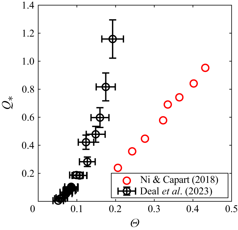
 Θ
 Q∗
 Θ≈0.2
 Q∗
 6
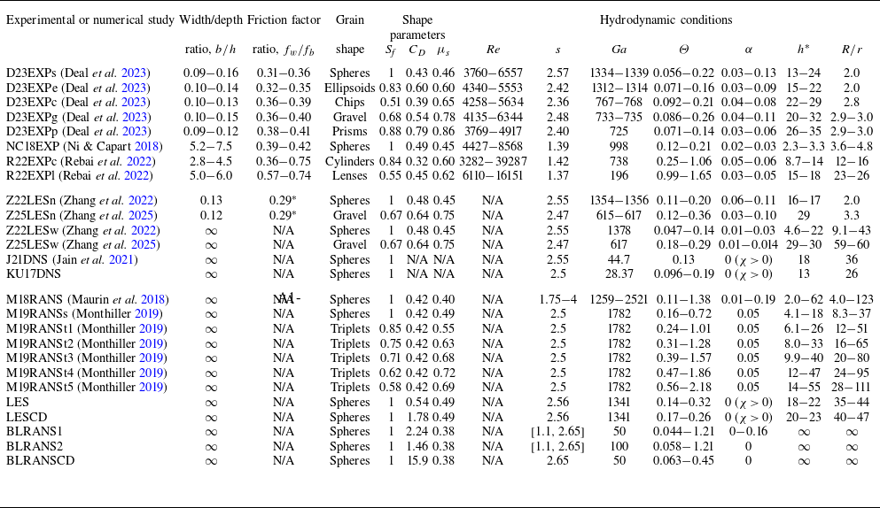
 s=2.65
 α=0
 ∗
 fw/fb
 CD
 Ga
 Θ
 h∗
 d=cg
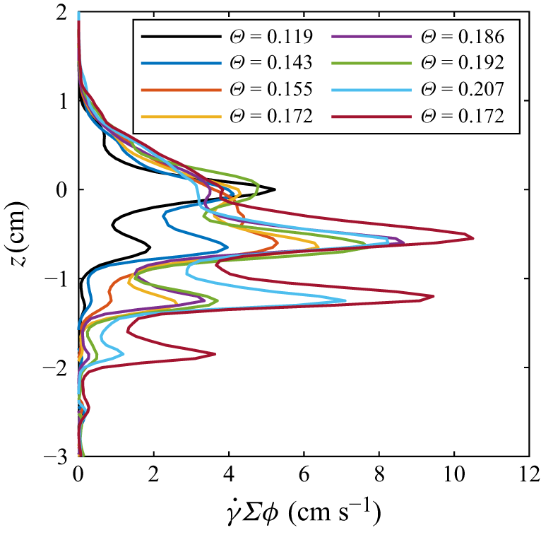
 γ˙Σϕ
 σzxf(z)
 σzxf(0)≈τt
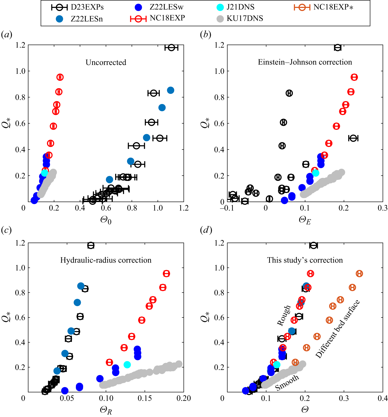
 Q∗
 Θ0
 ΘR
 ΘE
 Θ
 s1/2Ga≈44.86
 s1/2Ga>70
 h
 τb
 ∗
 h
 h≫d
 Θ=3ΘR
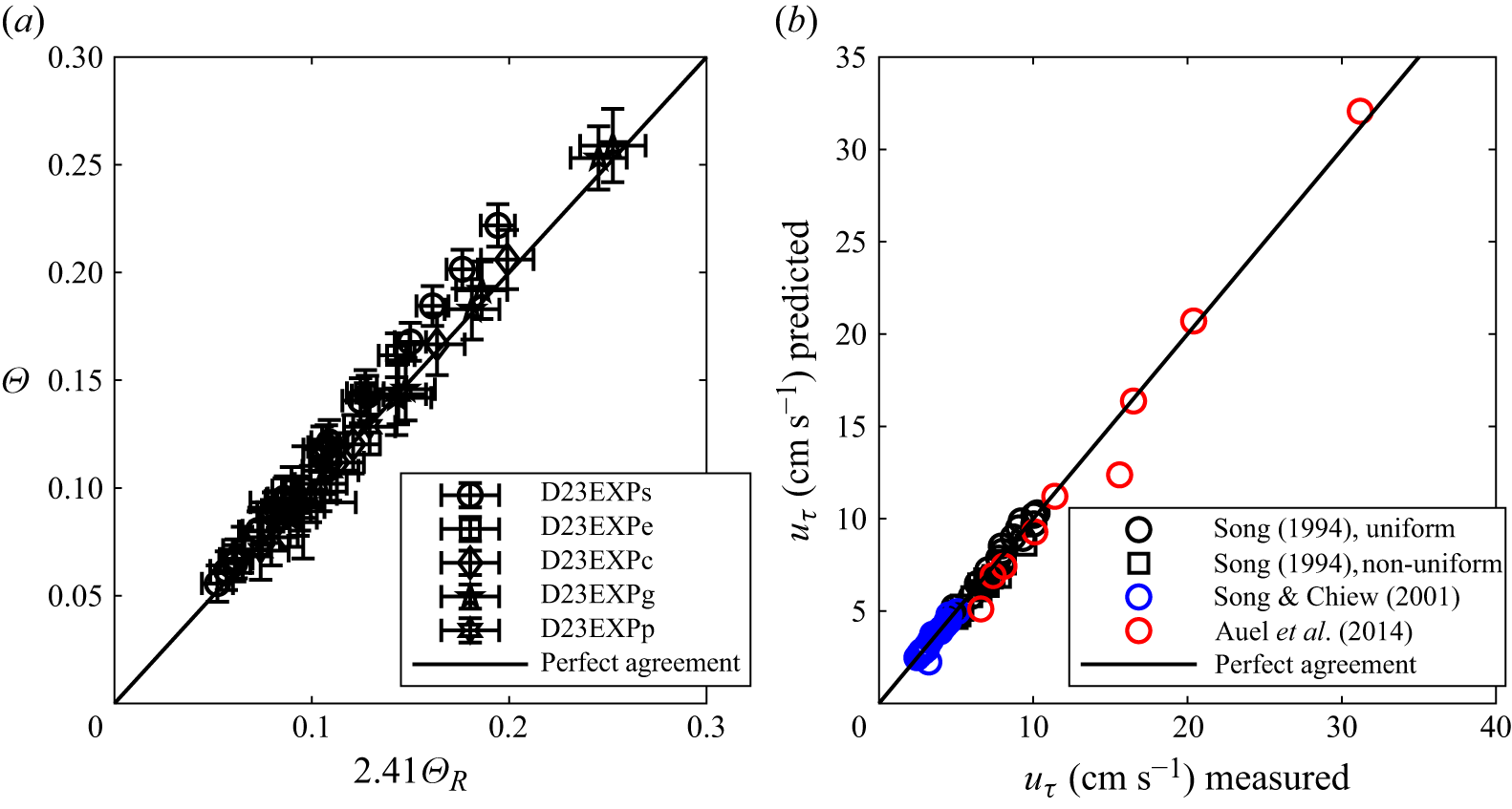
 Θ
 2.41ΘR
 d=cg
 τb=2.41τR
 uτ≈τb/ρf
 r=d0
 r=k
 tanα
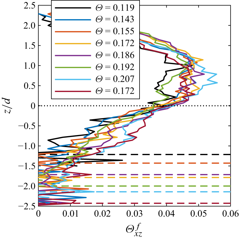
 Θzxf≡σzxf/(ρpg~zd)
 z=0
 Θzxf(0)≈0.04
 σzxf
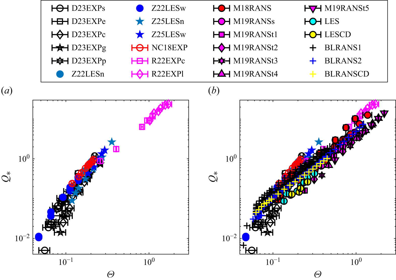
 Q∗
 Θ
 d≡(3/2)Vp/Apmax
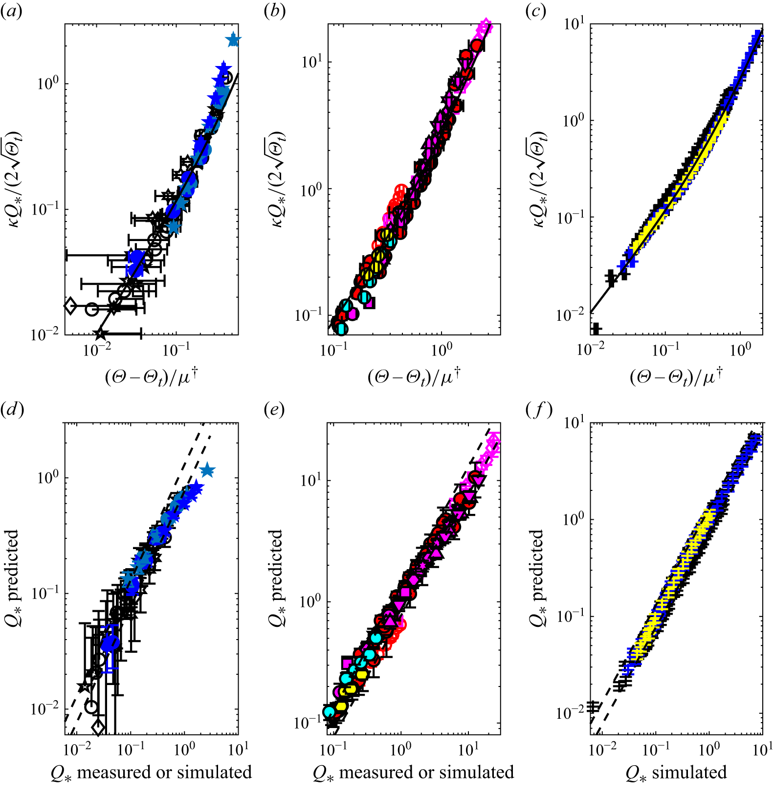
 Y≡κQ∗/(2Θt)
 X≡(Θ−Θt)/μ†
 Y=X(1+cMX)
 Q∗
 Q∗
 s1/4Ga⩾200
 Θt
 Θt
 fL¯/fD¯=0
 1.3

 Q∗D23
 ΘD23
 (C∗/μ∗)ΘD23
 Q∗D23=12(ΘD23−0.05)3/2
 Q∗D23=12(ΘD23C∗/μ∗−0.05)3/2

 μs
 25000
 2d
 90∘

 μs
 do
 24do
 2do
 90∘
 A
 A≲2
 μs
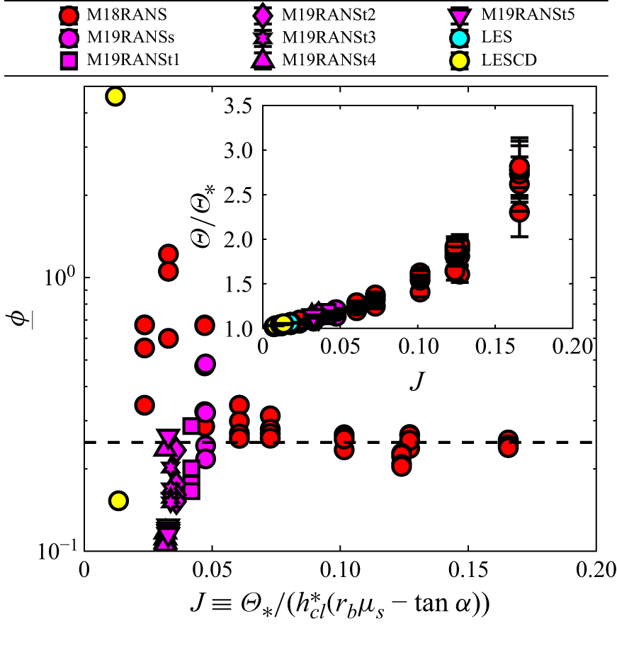
 ϕ_
 Q∗
 J
 ϕ_=0.25
 J
 Θ/Θ∗
 Θ/Θ∗
 ϕ_=0.25
 μs
 M∗
 Θ


