The Importance of Family Space

There are practical reasons for studying family dispersion. The availability of family members to support the elderly is just one example because support also goes from older to younger members, and some of it, such as care of grandchildren, requires spatial proximity. Welfare systems now use the term kinship care to refer to the placing of grandchildren with their grandparents (or other kin) if they have to live apart from their parents (e.g., Iglehart Reference Iglehart2004). The presence of kin nearby (or far away) is also important in how a community responds to disasters and is included in measures of resilience.

The presence of kin also affects demographic outcomes (e.g., Broström et al. Reference Broström, Edvinsson and Engberg2018; van Djik and Mandemakers Reference van Djik and Mandemakers2018). Did having a mother-in-law nearby affect the fertility or infant mortality of her daughter-in-law? Recently, Hacker and Roberts (Reference Hacker and Roberts2017) studied the effect of having a mother-in-law nearby upon fertility. They used a proxy measure—whether a woman with the daughter’s surname lived within the closest 10 households on the US 1880 Census and found a relationship. In many societies, a patrilocal pattern of residence led to pressure from the mother-in-law for her daughter-in-law to have children. Her presence might also affect child mortality by way of resources made available or other means. Frequently, however, these studies do not consider the underlying reasons for proximity of kin. If resources are attractive, kin may remain together. Beneficial outcomes could come from the plentiful resources not the presence of a grandmother. The study of the factors leading to kin proximity would provide a “control” for some of the oft-claimed benefits. But because we know so little about kin networks in space, it is difficult to use them in modeling outcomes.

While fathers’ and sons’ incomes have been found repeatedly to be correlated in contemporary studies in many countries, and there is also research on effects of more distant kin (Song and Campbell Reference Song and Campbell2017), such correlations could arise from relatives living near each other, not because of any “inheritance” of wealth. Mobility studies acknowledge variation between countries, but there is very little attention paid to how spatial patterning within countries could affect results. Some studies include very simple spatial variables: whether the parent or grandparent was an immigrant or the region of the country where the individual lived. Some studies do include the possibility for social interaction between the parent or grandparent and the person whose wealth or income is being explained. Although there are methods that can be used to explore and include different possible spatial effects in multivariate models (Anselin et al. Reference Anselin, Florax and Rey2010, who uses numerate methods; Lawson Reference Lawson2009, who uses Bayesian methods), studies of social mobility in the past and the present have not made use of them.

Our analysis of family effects upon wealth using the nineteenth-century-Yankee data showed that in 1860 brothers’ wealth was related even after the father had died. The analysis controlled for the spatial proximity of the brothers and included several different spatial effects upon wealth (Kasakoff et al. Reference Kasakoff, Lawson and van Meter2014). We also modeled wealth longitudinally for three census years, 1850, 1860, and 1870, to test for family as well as temporal and spatial effects (Kasakoff et al. Reference Kasakoff, Lawson, Dasgupta, Feetham and DuBois2018) and did not find such family effects. A peak year for wealth of farmers in our data was 1860. Such effects might come and go depending on economic and political conditions, such as the Civil War, which occurred during the period we studied.

The migration patterns leading to clustering of relatives may also affect the development of cultural regions. If regions are defined by social interaction, family ties should be clustered within them. Fischer (Reference Fischer1989) traced such cultural regions in the colonial United States to the origins of the colonists in different parts of Europe. And there are indications that such regions persist.

Conceptualizing Family Space

Despite its importance for social support, mobility, and the “social fabric,” the clustering and dispersion of relatives in space has rarely been studied as a process on its own. There are, however, some concepts useful for understanding it.

Rosental (Reference Rosental1999) discussed the “family territories” of people living just outside the reach of Paris. His data came from family trees collected in the TRA project (Bourdieu et al. Reference Bourdieu, Kesztenbaum and Postel-Vinay2014). He contrasted families that were auto-centered (“rooted” in a family territory) as opposed to exo-centered (oriented to outsiders), measured from the degree to which witnesses to marriages were repeated within a family tree. Rosental (Reference Rosental1999) also showed how family ties through sisters were used to secure jobs for their brothers when they moved from rural areas. The sisters, then, had a family territory that linked the rural areas where they were raised with the larger settlements where they were living later in life and linked their natal families with their husbands’ networks. The family territory exists at a “meso level” between the local commune and the nation-state (Adams et al. Reference Adams, Ericsson, Page Moch and Kok2002a: 129).

Kesztenbaum (Reference Kesztenbaum2008) used the TRA data to measure spatial capital. He built upon Levy’s (Reference Levy2003) expansion of Bourdieu’s notion of social capital to include space. Levy pointed out that while migrants may be poor, they have a great deal of spatial capital, that is, they link many places together (Levy Reference Levy2014). Also, spatial capital could be turned into other forms of capital. The places where a family lives and has lived in the past represent a stock upon which people could draw in their own choice of destination. Kesztenbaum (Reference Kesztenbaum2008) calculated the number of places in lineages for TRA project trees and used this in analyses to determine the probability of migration. The past paths did not seem to influence migration. However, the idea that a family shares spatial capital is quite important: People draw on it today at times of crisis and when moving over long distances.

Hubs are “highly connected nodes” (Barabási Reference Barabási2014: 58) within networks. But if we move away from individual locations to a network, a hub could be an area where family members are concentrated. Barabási noted that when networks are plotted by size there are often a few large hubs and a long tail of small ones. He attempted to model the process that produced this structure using two principles: growth and preferential attachment. Growth means the network has a history because the earliest nodes have the longest time to grow. But this was not sufficient to explain the concentration of ties. He needed also preferential attachment: People prefer to link to people who are already linked. Like a gravity model in geography, people move to places with the most people. In later models he also incorporated age: As they age and have fewer roles in film, for example, actors do not link as much to other actors. Similarly, the first hubs become less attractive as networks age. This would certainly apply to situations such as pioneering where areas fill up.

Family trajectories can be useful in explaining how dispersion of relatives comes about. A trajectory is a sequence of statuses or roles a person occupies in his or her lifetime (Kok Reference Kok2007). How does the timing of migration during the life course affect the spatial distribution of relatives? If different societies or historical periods have different patterns of life course migration (and reproduction) how might that affect the formation and duration of family hubs? Life course studies incorporate the concept of “linked lives” to show how decisions of some family members affect those of others, but to see how spatial dispersion of families occurs, the trajectories would have to move beyond a birth cohort to include sequences of trajectories of individuals in different generations.

Yankee Genealogical Sample

Family trees are useful for studying the process of family dispersion, but only if they show the entire set of relatives, not just, for example, a line going back through only one individual each generation without including their siblings and the children of those siblings. Other advantages are that the linkage has already been done, at times with the aid of information privy only to family members. They allow the study of processes over many generations and thus long-term outcomes (Grusky et al. Reference Grusky, Smeeding and Snipp2015; Mare Reference Mare2011; Ruggles Reference Ruggles2014; Song and Campbell Reference Song and Campbell2017). However, these processes must be anchored in space. If the data gives locations, they allow an analysis of spatial dispersion along with temporal change.

We began the Yankee Genealogical Sample in 1977. We thought it important anthropologists study regions of interacting villages, not single isolated villages. After exploring marriage ties as an indicator of regional interaction in a variety of societies using secondary literature (Adams and Kasakoff Reference Adams and Kasakoff1975), we realized that because there is so little historical data on the societies that anthropologists study, we would have to find other sources to explain how the territorially rooted “endogamous groups” developed over time.

We decided to use information from published genealogies and created a database designed to document the migration of family members whose lives were described in nine such books. We selected families in which the founder came to New England before 1650, when almost all the progenitors of what later became the Yankees came. After 1650, migrants from England went to the Middle Colonies, so New England was nearly a closed population expanding only by natural increase (Matthews Reference Matthews1962). We thought the migration paths of the families would be influenced by where they first settled, so we picked three families whose founders settled in the middle of Massachusetts (Farwell, Pelton, and Coney were chosen because they moved to a city, Boston), three who went to what was Plymouth colony or other parts of Southern Massachusetts (Bisbee, Faunce, and Chaffee), and three whose founders had died in Northern Massachusetts (Greely, Wellman, and Shed). It turned out that once they moved into New York in the early nineteenth century their migration paths did not vary a great deal. However, Chaffees did move up the Connecticut River near where they had first settled, and Bisbees and Faunces moved from Plymouth to Maine.

We used a guide to surnames that were present in the American colonies prior to 1650 (Colket Reference Colket1975, which gave stars to high-quality genealogies). Colket was a founder of the American Society of Genealogists in 1940 and an advocate for a more systematic and scientific approach to genealogies (Weil Reference Weil2013: 169). Our criteria included that women had to be followed along with men. We also looked for books that contained more than just the begats: First and foremost, we wanted specific locations of vital events as well as information about occupations. We also chose books that documented their sources.

These genealogies came out of a democratic movement in the nineteenth century: “[A] new genealogical regime dominated by middle-class, family-related, republican moral concerns” that stressed the “family as a moral, social, and political unit in the new republic rather than the elite status oriented concerns that prevailed during the Colonial period” (ibid.: 43). “The humblest artisan or laborer, who partook in the glorious work of peopling our N.E. world, should be secure of his commemoration as much as Govrs. Winthrop, Haynes or Eaton” (James Savage writing in 1806 quoted by ibid.: 70). These democratic genealogies emphasized ordinary descendants over distinguished ancestors. They were also descending genealogies rather than pedigrees (see following text). But the effort was also fueled by a desire to promote the Puritans and Pilgrims who settled New England as the first true Americans. It was also probably no coincidence that during the 1840s, when the New England Historic and Genealogical Society was founded in Boston, many Irish were moving there. The genealogical movement was a “Nativisitic” movement (Linton Reference Linton1943) and genealogies furnished “proof” that the descendants were here first.

Family reconstitution was being used in the United States to understand the lives of ordinary people in colonial America, resulting in several “town studies.” In some ways, they were adopting the closed single village of anthropology that we thought should be abandoned. Using data from family trees, we were able to critique some of those central tenets of family reconstitution: Migrants were not the same as those who remained behind and that, furthermore, at least in colonial America, they formed a considerable proportion of the population. Family reconstitution should underestimate ages at vital events such as marriage and death because people who left the village and experienced those events elsewhere were not counted (Adams and Kasakoff Reference Kasakoff and Adams1995). While Henry, who originated family reconstitution, had proposed ways to compensate for this, such as including in-migrants, they were frequently not used, even impossible because the ages of the in-migrants might be missing as they had not been born there.

Because of the rapid rate of increase of the population in colonial New England, Malthus used this population as an example of what could happen if fertility did not decline. Indeed the population increased quite rapidly—on average four sons lived to have sons. The Yankee database includes about 25,000 individuals. We entered all individuals, male and female, born in the patriline up to 1840, all their children and siblings, and the spouses of the men. The nine progenitors had produced some 1,464 men 25 or older whom we were able to locate on the census of 1850. We have since linked the men in these families to the US censuses of 1850, 1860, and 1870. This group went on to become known as the “Yankees” and the map of where the Yankee sample lived when Lincoln was elected coincided with the map showing counties that had voted for him. It is thus a record of an ethnic group that came to settle the entire Northern tier of the United States.

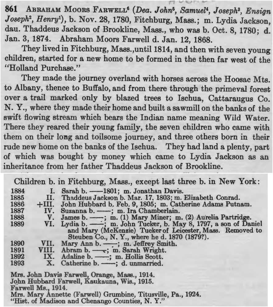
The example of the family of Abram Farwell in figure 1 (Abbott and Wilson Reference Abbott and Wilson1929: 151–52) illustrates the richness of the materials and the migration patterns typical of these families. He was born in 1780, just after the Revolution in Fitchburg, Massachusetts, where his father had moved after marriage. It was 28 miles from Chelmsford, where the founder of this family settled in 1655. But in 1814, Abram became the first European settler in Ischua, Cattaraugus County, New York (French Reference French1860), some 500 miles away. He moved with seven children and had other children after arrival. Did he wait until his oldest son was old enough to help clear land—which makes sense due to the lack of labor on the frontier (Adams and Kasakoff Reference Adams and Kasakoff1984)? Maybe so, but in this case his move seems to have followed the death of his wife’s father as the genealogy specifically notes they used that money to purchase land.

Figure 1

Abraham Moors Farwell entry from genealogy.

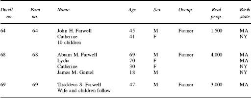
By linking to the census we can add occupation, wealth, and household arrangements. In 1850—the first US census to list every inhabitant by name and household—Abram, age 70, is surrounded by kin (see table 1). The large tract of land he had purchased earlier had been divided into farms for his several sons. But by the 1870 Census, Abram has died, his wife Lydia is living with Catherine, her unmarried daughter (and is “insane,” not the energetic pioneer the genealogy talks about), close to her sons. They were all doing very well economically.

Table 1

Abram Farwell, 1850 Census, Rice, New York

Source: Ancestry.com, 1850 census.

This genealogy was published in 1929, but as early as 1914 the compiler, John Dennis Farwell, was corresponding with family members as far away as Wisconsin and Pennsylvania to fill in gaps and follow the family farther West. In the original book, only one son was followed in the next generation (entry with a plus sign). Nevertheless, we have added information on the other sons and their children from censuses.

Abram’s story was repeated over and over in the nine families, which during the nineteenth century settled the Northern tier of the United States (Matthews Reference Matthews1962). They traveled along latitudes partly because the variety of corn they had could not grow farther south or north (Steckel Reference Steckel1983). The modern varieties that do not have such strict limits were not developed until much later. Cultural regions followed such latitudinal bands as well, at least until they reached the Great Plains (Fischer Reference Fischer1989; Woodard Reference Woodard2011), and these migration patterns were the basis for regional dialects. These regions are remarkably persistent: We have documented the same latitudinal bands using Twitter from 2013 (Huang et al. Reference Huang, Guo, Kasakoff and Grieve2016).

The Development of Families in Space

Family Hot Spots

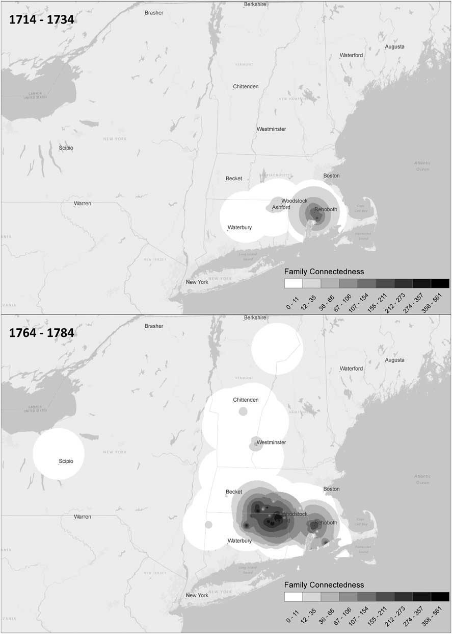
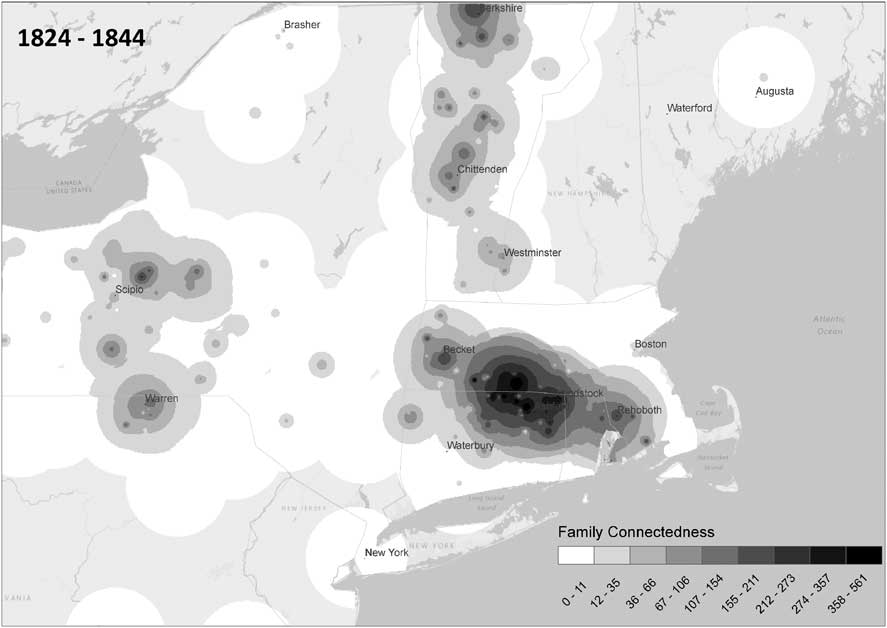
We created a measure of kin density and plotted it over time for the largest family in our database, the Chaffee family (Koylu et al. Reference Koylu, Guo, Kasakoff and Adams2014). For each individual, we looked for all the other men descended in the male line within a 60 km radius (37 miles), the median distance of a move in our data. We used only men because of the difficulties following women in genealogical data (see figures 2 and 3). We weighted each by the length of time they had been within this radius (using 20-year periods that overlapped) and also by the closeness of the relationships between individuals. We did this only out to first cousins. We summed this number for all individuals and the result was a surface of kin density or family connectedness (the darker the shade, the more intense the kin relations). The darkest areas represent hot spots, areas where kin ties were concentrated. They represent episodes of successful pioneering. This surface describes the potential for interaction. We know very little about actual interaction. But it is certain that it was much easier to interact within the 60 km radius than beyond.

Figure 2

Chaffee family connectedness: 18th century.

Figure 3

Chaffee family connectedness: 19th century.

One hundred years after the first Chaffee arrived in Massachusetts, the hot spot located around the town they first settled, near the Connecticut River, was still the most prominent, even though, by then, the family had also spread out to nearby towns. The balance of kin between the component towns in this cluster changed, sometimes quite rapidly, due to the deaths of grandfathers who linked people in different towns. This family moved up the Connecticut River to Vermont. Between 1760s and the 1820s, they branched out to several areas of New York State and to Maine, but the original location became hotter and had the highest density of kin throughout the nearly 300 years of data, still the largest concentration of kin even in 1914 when our data ends.Footnote ¹

The rapid growth of the early generations, which lasted for more than a century but remained within a very small physical area, was never again duplicated. Even as people moved out and established family branches elsewhere, they tended to leave before equally dense family hot spots could be established. Concentrations of kin sometimes diminished in strength as family members left and disappeared altogether. It took several generations in one place to create the enduring hot spot at the family hearth.

When we plotted all nine families together, the diagrams did not show these patterns as clearly. The concentrations became closer to population density, but not the same. If we had controlled for actual population density, the result would show what is really a family, and not a population pattern, a set of family hubs or hearths, representing similar colonization episodes, where each of the original towns was founded.

These surfaces make visible patterns that we could not have seen before: They are visualizations of a family territory over several generations. Each one can be treated as an object, the residue of many forces or processes. These processes explain the different forms such a surface took in historical contexts. It is a footprint of a family’s successful migrations, in the form of relatives who remain in places where the family lived, on its way to being extinguished as people die, and there are no descendants in those locations.

Proximity of Fathers and Adult Sons: 1850 vs. Today

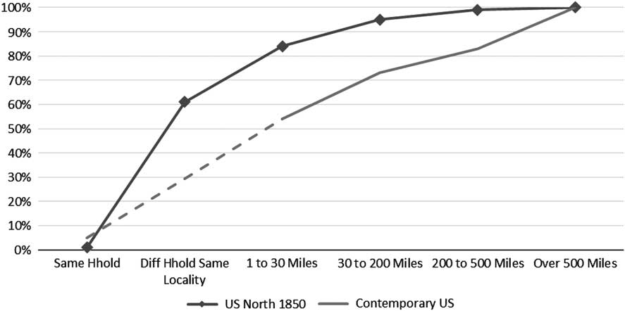
It is only in the last few years that information has been available for the United States that could be compared with the family trees that I have been studying. The most complete study so far uses data from PSID (ibid.), which in its last survey asked the person being interviewed about the whereabouts of their child and their parents. Here I will compare the findings of this survey about the proximity of fathers and adult sons with the Yankee Genealogical Sample in 1850 (see figure 4). The contemporary study uses 30 miles as a threshold, a distance that one could travel in one day by car. The comparable distance in the nineteenth century was less: 73 percent of adult sons were living within 15 miles of their fathers in 1850. Twelve percent lived more than 120 miles away, much of this representing pioneering, but I use the 30 miles to facilitate comparison (see Supplementary Materials).

Figure 4

Distances between fathers and their closest adult son in 1850 US North.

Eighty-four percent of men with living adult sons had at least one within the 30-mile radius in 1850 but only 54 percent have sons that close to them today (see Supplementary Materials for the sons’ perspective). Sixty percent of the men had sons in the same locality (this number is not available for the contemporary data). This chart, and the table that follows, includes only men who had at last one son age 25 or older. That would mean the fathers in question were at least 45 years old. If we were to also add those men who did not have any adult sons, the number with no son within 30 miles would be larger in both populations. Differences in demographic availability are not easily explained because the two populations differed so much in age structure and the contemporary data is not broken down by age.

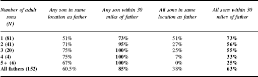
Whether one had a living son close by depended very much on how many living sons the father had, as table 2 shows. Among men with only one surviving adult son, 73 percent lived within a 30-mile radius of him. But among men with two, 93 percent had a son this close by and all the fathers with more than two sons had at least one within the 30 miles. The more sons, the less likely they would all live within a 30-mile radius of their fathers.

Table 2

Proximity of adult sons to fathers in 1850

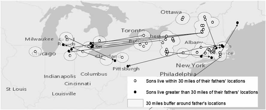
Figure 5 maps fathers and their adult sons in the Chaffee family in 1850. Solid dots are sons living within 30 miles of their fathers, and we have joined the family territories together if they overlapped. They are quite similar to the hot spot maps referred to previously from an earlier period, though we are focusing on only one relationship. We see the hub in southern Massachusetts, the family hearth, and another in Vermont and New York. And these maps follow the process westward.

Figure 5

Map of fathers and sons: Chaffee family 1850.

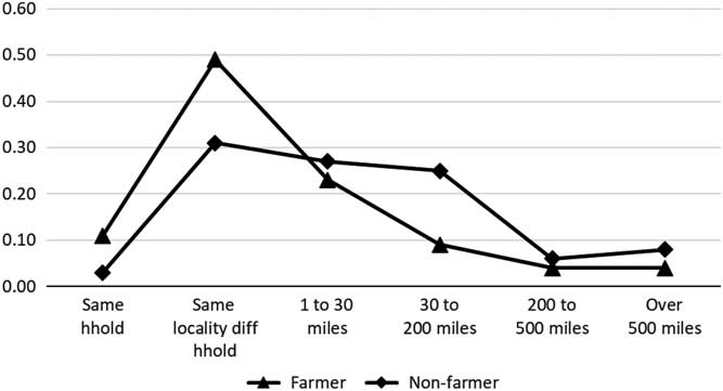
Arrows linking sons to their fathers more than 30 miles away represent the new opportunities; the tip of the arrow is the son’s location and the other is the father’s (see figure 6). There were six cases of pioneering, largely in Michigan but also in northern Pennsylvania. But the majority of sons more than 30 miles from their fathers were not farmers. Occupation was important then and probably today as well; Choi (2018) reports that the more education the child has, the farther a son lives from his parents. As people left farming, there would be greater spatial dispersion. But as fertility declined, at least among farmers, there would be a contrary pressure for at least one son to remain behind to work the farm, which required two men, and care for parents in old age.

Figure 6

Distances of sons from fathers by son’s occupation in 1850.

There is evidence that family clusters continued in the next generation: There were three examples where brothers moved more than 30 miles to new locations without their fathers. Two were cases of pioneering in Michigan and, in a third case, two sons of a wealthy merchant in Newport, Rhode Island, set up branches of the business in South Carolina. In neither case was the father left without family in the older area. There is also ample evidence in the Yankee genealogies for brothers-in-law moving to the same locations. Usually the youngest sibling remained behind (and also inherited the farm), but the pattern varied by family size (Kasakoff Reference Kasakoff2010). We are analyzing the potential for interaction, not the quality of relationships. Still one should say that in the northern United States, families were so large that there was plenty of opportunity for falling out without depriving a father of a nearby son. Today the number of fathers with an adult son so close is perhaps more than one would expect, 54 percent. In at least some cases, both today and in the nineteenth century, the direction of support might run from parent to child if a child were unable to be self-supporting, and this might be more frequent now than it was in the past.

Social class plays an important role today. The professional classes have quite dispersed kin networks, although people in professions, like teaching, which require state credentialing, live closer to their kin (Lundberg et al. Reference Lundberg, Pollak and Stearns2016). The difference in proximity to relatives is only one of several class differences, which include age at childbearing and whether couples marry at all, which are becoming more pronounced. What poor people lose by not being able to marry, they may make up by remaining close to their original families. Family effects on social mobility will vary by occupations and educational strata. In the nineteenth century, farmers would not have to travel far to have their fathers’ help and their wealth could be correlated simply because they lived in the same vicinity under the same agricultural conditions. However, if a man left farming to live several miles away and his wealth was still correlated with that of his father, the explanation would have to be different.

Big Data from Crowd-Sourced Family Trees

Four databases that have recently been used to study population clustering give us a taste of the future. Two of the four databases link genetic information from a smaller population to a much larger set of “demographic” data (frequently genealogies) to identify spatial clusters. The Ancestry group uses 777,000 primarily US-born individuals who ordered DNA tests and consented to participate in research and linked them with a much larger data set of user-generated pedigree data to infer the history of the genetic clusters they identified (Han et al. Reference Han, Carbonetto, Curtis, Wang, Granka, Byrnes, Noto, Kermany, Myres, Barber, Rand, Song, Roman, Battat, Elyashiv, Guturu, Hong, Chahine and Ball2017). Kandt et al. (Reference Kandt, Cheshire and Longley2016) also started with genetic data from a small group, 2,039 volunteers in Great Britain whose four grandparents were born within an 80 km radius, and then linked it with a large data set, the 1881 census. The year 1881 was about the time when most grandparents of the genetic sample were born. They used only rural areas (18 million individuals, roughly half the population of Great Britain) and the study compared the regional clusters from the genetics with clusters of surnames from the census. The study was explicitly trying to test Pooley and Turnbull’s (Reference Pooley and Turnbull1998) conclusion from pedigrees that most migration in rural areas in Great Britain was over quite short distances. Two other projects created even larger data sets from user-generated trees: Geni.com (Kaplanis et al. Reference Kaplanis, Gordon, Shor, Weissbrod, Geiger, Wahl, Gershovits, Markus, Sheikh, Gymrek, Bhatia, MacArthur, Price and Erlich2018) yielded 86 million individuals and Rootsweb.com (Guo et al. Reference Guo, Kasakoff, Koylu, Huang and Grieve2015), which I will refer to as the Trees data set, 80 million. Geni has more individuals from outside the United States.

Spatial clustering techniques applied to these Big Data sets revealed regional boundaries, migration, and large-scale temporal changes that would affect proximity to kin. Not surprisingly, because urban areas were excluded, Kandt et al. found there were relatively stable regions in Great Britain where surnames and genetics corresponded. It is difficult to evaluate the scale of genetic differences, but Great Britain, a much smaller geographical area than the United States, was divided into much smaller geographical regions than the United States in the nineteenth century. The spatial patterns from the United States from Ancestry confirm what is known: Acadians live in Louisiana and the eastern part of the United States has clusters that correspond with east-west bands. That these studies confirm well-recognized patterns validates this type of data.

But there is also potential to find new patterns and pinpoint the timing of changes. The Geni study documented changes in the distances between birthplaces of parents, children, and spouses. It has always been thought that these increased over time, but these studies confirm them on a grand scale and also suggest turning points that have yet to be fully explained historically. Distances between birthplaces of spouses increased in both Europe and North America after 1750 (marriage date), but, as one would expect simply from differences in population density, as well as earlier research, European distances were always smaller than in the United States. Only in 1950 did the two catch up to each other (Kaplanis et al. Reference Kaplanis, Gordon, Shor, Weissbrod, Geiger, Wahl, Gershovits, Markus, Sheikh, Gymrek, Bhatia, MacArthur, Price and Erlich2018: supplementary figures 18 and 19). There was a lag between the increase in spousal distances and a decrease in genetic relatedness, and the authors speculate that people continued to marry relatives even after changes in mobility that produced greater mixing.

Distances between birthplaces of fathers and sons started to increase in 1850 in Europe but did so earlier in the America. This increase could not have been due to immigration because only native-born sons and fathers were included. Kaplanis et al. (Reference Kaplanis, Gordon, Shor, Weissbrod, Geiger, Wahl, Gershovits, Markus, Sheikh, Gymrek, Bhatia, MacArthur, Price and Erlich2018) attributed the increasing distances to the railroad. But the increased distances could reflect moves before 1850 because the average time between the birth of a father and his son is 30 years. Urbanization and nonfarm work were more likely causes. A spatial analysis at a smaller scale would identify more clearly where people moved and help explain why these distances increased.

Big Data will allow researchers to study spatial dispersion of families in many different social contexts, to see how large-scale changes such as the demographic transition, transportation changes, urbanization, immigration, and the like affected family networks in space. But studies have yet to address the issues of representativeness or accuracy in a thorough way. Changes over time may reflect changes in the sources, samples, coverage, and so forth. There are many reasons to suspect that the data are less complete and less accurate further back in time.

Limitations of Genealogical Data

Written Sources and Linkage

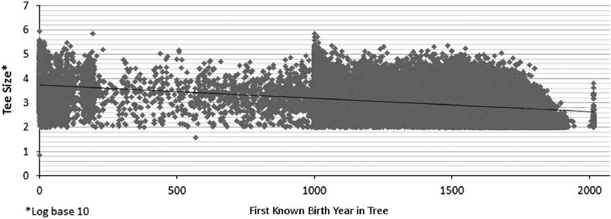
Despite the enormous numbers of individuals in these data sets they are all limited by the availability of written sources and difficulty of linkage. Dating and naming and writing each has a history that affects the very possibility of being included in a genealogical data set. We plotted the Tree data set by the number of individuals in the tree (vertical axis) and the date of birth of the founder (see figure 7). We wanted to know whether trees that went further back in time were larger. The answer was yes, but the results showed how genealogies depend upon written sources. For an individual to be in a tree, he or she needs a name and a date that has been preserved (note: figure 7 uses birth dates). The Franks were the first in Europe to satisfy this criterion, so it is not surprising that the earliest founder in the data was Otamir the Great, a Frankish king. There are a large number of trees in which the earliest individual was born before 200 AD, but they probably all go back to such early royal families. The years from 200 to 1000 were a “dark age” when many fewer trees began, likely because of the paucity of written sources. Many more trees began after 1000.

Figure 7

Tree size by first known birth year.

Societies differ in the uniqueness of names, and this also imposes limits on trees. Commonness of names drastically reduced the linkage rate in the IPUMS USA linked sample (IPUMS USA 2010). If, as has been shown for the United States (Olivetti and Paserman Reference Olivetti and Paserman2015; Olivetti et al. Reference Olivetti, Paserman and Salisbury2016), complexity and length of names is associated with a higher social class, then there will always be a problem of linkage for the poorer people in the population and genealogical data sets will be biased toward the more wealthy in the population.

Comparison with Census Data

One way to assess representativeness is to compare with a census. We compared the men in the Yankee sample with the census data for a comparable group taken from the IPUMS sample from 1850 (Ruggles et al. Reference Ruggles, Genadek, Goeken, Grover and Sobek2015). We took a sample of households containing native-born men 20 years of age or older born in each of the states where our sample was concentrated: New England, New York, and the Middle West. It was impossible using these criteria to exclude some of the more recent arrivals: children of German and Irish immigrants who had been born in the United States. Despite the longer time they had lived in the United States, the men in the Yankee sample were only slightly more wealthy than the IPUMS sample. And, part of the reason, as expected, was that the IPUMS sample was less likely to be farmers (Kasakoff et al. Reference Kasakoff, Lawson and van Meter2014: 8).

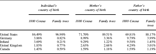
The Trees data lack foreign born. Ninety-seven percent of the individuals in the trees had been born in the United States whereas only 86 percent of the US population in 1880 had been born there (see table 3). The greatest deficit is for the Irish. New York was the state with the greatest difference in population between the two data sets, presumably because of the lack of Irish who were concentrated there (see Supplementary Materials). The duplication in their names and their concentration in cities would make it quite difficult to construct their trees. Likewise, the South and Midwest are somewhat overrepresented in the Tree data probably because fewer immigrants went to those regions. A regression on the difference between the Trees sample and the census for each state’s population in 1880 had statistically significant effects: Farmers are overrepresented in the Trees sample; blacks and foreign born are underrepresented.

Table 3

Comparison of 1880 Census and trees, proportion born in each country

But if the data is restricted to native-born children of native-born parents, the trees match the census proportions living in each state in 1880 almost exactly. The biggest discrepancies are in a few recently settled states where the Tree sample has too few people (see Supplementary Materials), most likely because they had moved there recently but our methods allocated them to their birth states instead.

Erlich et al. (Reference Erlich, Shor, Pe’er and Carmi2018) have found a similar bias in the Geni data. They estimate that 60 percent of individuals of European descent within the United States have a third cousin or closer relative in a publicly available genetic database who can be identified using identifiers from the Geni data such as place of residence, age, and sex. But 75 percent of the individuals who were matched were white. The linked IPUMS samples have a similar bias toward whites (IPUMS USA 2010) and native born. This is a serious problem that all users of Big Data must tackle in the future.

Uncertainty and Accuracy

Dates of the moves in genealogical data are too late because they are discovered only through vital events recorded in a “new” place. Also there are long stretches of the life course that we know little about because of lack of vital events. The longest period is that between the birth of the last child and the death of one of the parents. Leaving home is difficult to study. Short-term moves and circulation or return migration are invisible because even the closest spaced vital events, usually the births of children, in our Yankee data, a high-fertility population, are two years apart. Linking the trees to the decennial censuses can fill in missing information but only every 10 years. The new Big Data studies focus on parent-child birth distances because that is what is usually most available in genealogical data. This means the temporal resolution is only a generation—30 years or so. Therefore, it is difficult to see the impact of historical events, as we have seen in the attempt to explain increasing spousal distances.

The genetic data in some of these data sets allow an assessment of accuracy. The Ancestry study (Han et al. Reference Han, Carbonetto, Curtis, Wang, Granka, Byrnes, Noto, Kermany, Myres, Barber, Rand, Song, Roman, Battat, Elyashiv, Guturu, Hong, Chahine and Ball2017) matched genetic information from fathers and sons identified in genealogical data and found a rate of agreement that matched other studies. The Geni study validated the trees from genetic material they had on a small number of individuals (211 lineages through women and 27 through men). Accuracy could be assessed by matching individuals in trees with individuals in complete count censuses. In this case, however, it may be the census that is wrong, not the genealogy; one study has estimated that 18 percent of the birthplaces there are not correct.

The entry process for the user-generated data may also affect accuracy. Geni users are pointed to another profile that matches the person they are entering, and it is the user who makes the judgment that their relative is the same individual as the one already there. They are also asked to validate the geographical locations they enter. (Both Geni and Ancestry have what are probably the most complete global historical gazetteers in existence.) Users might not know which of several different place names or individuals match their relatives, so Geni data is probably better the closer to the present it is. The Geni study has “validated” its data through matching death dates with Vermont death certificates, but these constitute only a small proportion of their sample and only one variable of interest.

Rootsweb does not eliminate duplicates, so the Trees project had to clean the data to eliminate them. The 247,765,060 “individuals,” about five times the population of the United States in 1880, were reduced by two-thirds. Six percent of the trees were eliminated because they were either exact duplicates or of too poor quality to use. Thirty-six percent of the “individuals” were removed because they did not have a first and last name, birth year, gender, or birthplaces at state level in the United States and country level outside the United States. Twenty-eight percent were removed after a complex process of comparing married couples and their offspring to find duplicates. Despite all the pruning, these trees are representative of the native-born population in the United States in 1880. Still, we do not know if the links are accurate. This could be assessed by linking individuals in the trees with censuses and comparing information from the two sources.

Linkage methods can affect results. If there are false positives then individuals who are not “the same” are treated as such resulting in higher rates of both geographic and social mobility. One of the most common methods of linking names, Soundex, has been found to create many more false positives than a method based upon degree of divergence. One study found linkage methods can overestimate intergenerational income elasticities by 50 percent (Bailey et al. Reference Bailey, Cole, Henderson and Massey2017). Its conclusion relied upon using trained genealogists to assess the accuracy of matches.

The three Big Data sets each report one large cluster along with several smaller ones. These data sets undoubtedly overlap and include most of the individuals in the earlier, smaller, genealogical data sets. So far all the data sets share the same biases: white native born (in the United States) of European stock. All three have posed the challenge of including more people from diverse populations. There is another way of validating the trees: merge them to see if the data on particular individuals agree.

Contingency and Timing

Ingold (Reference Ingold2016) contrasts a fixed point connected by straight lines with “wayfaring,” a wandering or a braiding of paths. The former is part of the industrial age while the latter is preindustrial. The wandering view of a family tree considers duration and spatial extent, not just ancestry and descendants. I have tried to show how a family tree, and especially large numbers of them, can help us conceive of flows not points—flows that have durations and connections.

Even as patterns emerge from many family trees, they are particularistic, full of chance and accident (Foucault Reference Foucault1977). The massive effort to study spatial patterns through Big Data may lead to a greater understanding of how chance affects history. Each family hot spot map is unique, even though we can discern patterns and forces that create them. The spatial pattern of family relationships has the advantage of being visual, anchored in demographic events, even as it makes room for contingency and individual agency.

As Gordon-Reed (Reference Gordon-Reed2008: 78) has written about the children of Elizabeth Hemmings, mother of Sally, who had children with Thomas Jefferson: “[T]heir individual family lines followed nearly all the various trajectories of black life during the eighteenth and nineteenth centuries. Some in those lines would become free well before the end of slavery in America… whereas others would not. Some, facing the enormity of white supremacy, would reject their African ancestry; others would continue to embrace it. These various pathways were forged out of the circumstances of Elizabeth Hemmings’s early life.”

This sense of history as a branching process over time with dead ends and affiliation with different groups, influenced (by how much?) by early events in the process, is one that family trees encourage, and it meshes very well with the tension between contingent events and long-term trends. These trends are made up of individuals. Which ones are the early birds and how are those selected? Which follow along later and which are the hold outs? These questions can be asked not only of migration but also of other types of change.

How stable were family hubs? The smaller families of today leave much more room for contingency in their development than in the past. Mechanisms have certainly changed and help might be less reliable especially among the more educated with their much smaller and more dispersed families. The location of family hubs has always been affected by random events—where the first person came, that the person remained there and produced children—and, importantly, each location led to particular opportunities and pathways out, opportunities that are constrained in space.