1 Background and motivation
In the context of the worldwide research effort on magnetically confined fusion reactors, the description and understanding of a wide class of plasma instabilities is of great importance; the subsequent low-level turbulent flows have a strong impact on the efficiency of the energy confinement properties of the device. This work is devoted to the ion temperature gradient instability (ITG) in an axisymmetric magnetic field configuration of the type found in tokamaks.
The low collisionality of the plasma in the core of the device calls for a kinetic model of particle dynamics. Taking advantage of the spatial anisotropy and time scale separation brought forth by the strong confining magnetic field, the original six-dimensional kinetic description is reduced to the so-called five-dimensional gyrokinetic model (see Littlejohn Reference Littlejohn1979, Reference Littlejohn1982; Frieman & Chen Reference Frieman and Chen1982; Dubin et al. Reference Dubin, Krommes, Obermann and Lee1983; Sugama Reference Sugama2000; Brizard & Hahm Reference Brizard and Hahm2007; Hahm, Wang & Madsen Reference Hahm, Wang and Madsen2009; Wang & Hahm Reference Wang and Hahm2010; Abel et al. Reference Abel, Plunk, Wang, Barnes, Cowley, Dorland and Schekochihin2013). Even so reduced, accurate numerical simulation of the gyrokinetic model remains a challenging task, which has led to substantial research effort in the past decades, and to the development of numerous codes such as GYSELA (Grandgirard et al. Reference Grandgirard, Brunetti, Bertrand, Besse, Garbet, Ghendrih, Manfredi, Sarazin, Sauter and Sonnendrucker2006a , Reference Grandgirard, Sarazin, Angelino, Bottino, Crouseilles, Darmet, Dif-Pradalier, Garbet, Ghendrih and Jolliet2007, Reference Grandgirard, Sarazin, Garbet, Dif-Pradalier, Ghendrih, Crouseilles, Latu, Sonnendrücker, Besse and Bertrand2008), ORB5 (Jolliet et al. Reference Jolliet, Bottino, Angelino, Hatzky, Tran, Mcmillan, Sauter, Appert, Idomura and Villard2007), GENE (Jenko et al. Reference Jenko, Dorland, Kotschenreuther and Rogers2000; Görler et al. Reference Görler, Lapillonne, Brunner, Dannert, Jenko, Merz and Told2011), GYRO (Candy & Waltz Reference Candy and Waltz2003), GS2 (Dorland et al. Reference Dorland, Jenko, Kotschenreuther and Rogers2000; Jenko et al. Reference Jenko, Dorland, Kotschenreuther and Rogers2000) and GT5D (Idomura & Jolliet Reference Idomura and Jolliet2011).
We present here two codes devoted to linear stability analysis, which rely on a multi-waterbag model of the ion distribution function. This kind of approach, which allows for a notable reduction of the problem complexity, has been used with some success for plasma instabilities analysis in cylindrical geometry (Morel et al. Reference Morel, Gravier, Besse, Klein, Ghizzo, Bertrand, Garbet, Ghendrih, Grandgirard and Sarazin2007, Reference Morel, Gravier, Besse, Ghizzo and Bertrand2008, Reference Morel, Dreydemy, Berionni, Coulette, Besse and Gurcan2014; Gravier et al. Reference Gravier, Klein, Morel, Besse and Bertrand2008; Besse & Bertrand Reference Besse and Bertrand2009; Klein et al. Reference Klein, Gravier, Morel, Besse and Bertrand2009; Coulette & Besse Reference Coulette and Besse2013a ,Reference Coulette and Besse b ). We propose here the first extension of the model to the global analysis of ITG modes in toroidal geometry.
Section 2 is devoted to the description of the physical model, the multi-waterbag reduction as well as the building of the stationary state used as a basis for subsequent perturbation analysis. In § 3, through perturbation analysis, we obtain the linear initial value problem describing the short time evolution of the perturbation. The problem is then recast as an eigenvalue problem in the so-called ballooning representation. The resolution algorithm, based on a second-order asymptotic expansion, is presented. In § 4 we detail the numerical schemes used in the implementation of both the initial and the asymptotic eigenvalue problem. Numerical results are presented in § 5, for a particular set of initial conditions compatible with both methods. We eventually briefly discuss the issues remaining to be addressed in order to extend the range of applicability of the model.
2 Physical model
In the gyrokinetic framework, particle dynamics is described by the evolution of the gyrocentres distribution function
 $f(t,\boldsymbol{r},v_{\Vert },\unicode[STIX]{x1D707})$
, where
 $t$
is time and
 $\boldsymbol{r}$
spatial position,
 $v_{\Vert }$
is the velocity along magnetic field lines and
 $\unicode[STIX]{x1D707}$
the magnetic moment. We consider here a ‘full-
 $f$
’ model, i.e.
 $f$
encompasses both the background and perturbed part of the gyrocentre distribution function. As
 $\unicode[STIX]{x1D707}$
is by construction (Brizard & Hahm Reference Brizard and Hahm2007) an adiabatic invariant of the model, it may be treated as a parameter. For a given value of
 $\unicode[STIX]{x1D707}$
, the distribution function
 $f_{\unicode[STIX]{x1D707}}(t,\boldsymbol{r},v_{\Vert })$
, is solution of the gyrokinetic Vlasov equation
 $$\begin{eqnarray}\unicode[STIX]{x2202}_{t}f_{\unicode[STIX]{x1D707}}+\boldsymbol{V}_{GC}\boldsymbol{\cdot }\unicode[STIX]{x1D735}f_{\unicode[STIX]{x1D707}}+\left(\frac{\text{d}v_{\Vert }}{\text{d}t}\right)\unicode[STIX]{x2202}_{v_{\Vert }}f_{\unicode[STIX]{x1D707}}=0,\end{eqnarray}$$
where the nonlinear drift velocity is defined by
 $$\begin{eqnarray}\boldsymbol{V}_{GC}=\frac{B}{B_{\Vert }^{\star }}\left[v_{\Vert }\boldsymbol{b}+\frac{v_{\Vert }^{2}}{\unicode[STIX]{x1D6FA}_{CI}}\unicode[STIX]{x1D735}\times \boldsymbol{b}+\frac{1}{B}\boldsymbol{b}\times \unicode[STIX]{x1D735}{\mathcal{J}}_{\unicode[STIX]{x1D707}}\unicode[STIX]{x1D719}+\frac{\unicode[STIX]{x1D707}}{q_{i}B}\boldsymbol{b}\times \unicode[STIX]{x1D735}B\right],\end{eqnarray}$$
and the parallel acceleration as
 $$\begin{eqnarray}\left(\frac{\text{d}v_{\Vert }}{\text{d}t}\right)=-\frac{1}{m_{i}}\frac{\boldsymbol{B}^{\star }}{B_{\Vert }^{\star }}\boldsymbol{\cdot }(\unicode[STIX]{x1D707}\unicode[STIX]{x1D735}B+q_{i}\unicode[STIX]{x1D735}{\mathcal{J}}_{\unicode[STIX]{x1D707}}\unicode[STIX]{x1D719}),\end{eqnarray}$$
where
 $\boldsymbol{B}=B\boldsymbol{b}$
. The corrected magnetic field
 $\boldsymbol{B}^{\star }$
is defined by
 $\boldsymbol{B}^{\star }=\boldsymbol{B}+(m_{i}v_{\Vert }/q_{i})\unicode[STIX]{x1D735}\times \boldsymbol{b}$
,
 $\unicode[STIX]{x1D719}=\unicode[STIX]{x1D719}(t,\boldsymbol{r})$
is the electrostatic potential,
 ${\mathcal{J}}_{\unicode[STIX]{x1D707}}$
stands for the gyroaverage operator, whose application on any function
 $F$
depending on position
 $\boldsymbol{r}$
is defined by
 $$\begin{eqnarray}{\mathcal{J}}_{\unicode[STIX]{x1D707}}F(\boldsymbol{r},\ldots )=\frac{1}{2\unicode[STIX]{x03C0}}\int _{0}^{2\unicode[STIX]{x03C0}}F(\boldsymbol{r}+\unicode[STIX]{x1D746}(\unicode[STIX]{x1D709}),\ldots )\,\text{d}\unicode[STIX]{x1D709},\end{eqnarray}$$
where
 $\unicode[STIX]{x1D746}=\unicode[STIX]{x1D70C}(\cos \unicode[STIX]{x1D709}\boldsymbol{e}_{1}+\sin \unicode[STIX]{x1D709}\boldsymbol{e}_{2})$
,
 $(\boldsymbol{e}_{1},\boldsymbol{e}_{2},\boldsymbol{b})$
form an orthonormal basis and
 $\unicode[STIX]{x1D70C}(\boldsymbol{r},\unicode[STIX]{x1D707})=(2\unicode[STIX]{x1D707}/q_{i}\unicode[STIX]{x1D6FA}_{CI})^{1/2}$
with
 $\unicode[STIX]{x1D6FA}_{CI}=q_{i}B(\boldsymbol{r})/m_{i}$
.
The multi-waterbag approach that we adopt here relies on the conservative nature of the particle flow in phase space (Liouville invariant). We will first consider for simplicity a one-dimensional problem, where the dynamics is described by a Lagrangian
 ${\mathcal{L}}(x,v_{\Vert })$
, where
 $x$
stands for a generic spatial coordinate. Let us assume an initial condition for
 $f$
defined the characteristic function of some bounded volume
 $\unicode[STIX]{x1D6FA}$
in phase space, i.e.
 $f=1$
is constant inside and zero everywhere else. As the value of
 $f$
is preserved along the characteristics (particle trajectories), the evolution of
 $f$
can be retraced by following only the Lagrangian evolution of the boundary
 $\unicode[STIX]{x2202}\unicode[STIX]{x1D6FA}(t)$
. The conservation of the volume of
 $\unicode[STIX]{x1D6FA}$
with time, while its boundary is deformed, led to the ‘waterbag’ denomination. Considering now for
 $f$
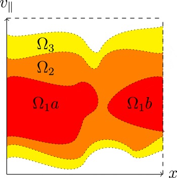
an arbitrary initial condition, it is always possible to decompose it as a (possibly infinite) weighted sum of individual waterbags (cf. figure 1) with completely decoupled dynamics. From a numerical point of view, the approach has two main potential advantages: first the evolution of all waterbags can be treated in parallel. Second, the most salient features of the dynamics can often be captured using a rather low (typically 5–15) number of waterbags. The price for those benefits is the requirement of Liouville invariance. This means first that a full-
 $f$
treatment is mandatory, and second that the model does not lend itself naturally to the treatment of collisional processes. Applying a collision operator strictly requires a full resampling of the multi-waterbag distribution. If one used a splitting scheme alternating a sufficiently large number of collisionless steps with the application of the collision operator, the additional numerical cost of the collision step should be bearable. In the following analysis we will consider a vanishingly small perturbation of the ion distribution function around a fixed local Maxwellian equilibrium so that a collisionless model for the fast evolution of the perturbation is a reasonable approximation.
Generic waterbag decomposition of the initial condition; three levels are considered here leading to four waterbags.

It is important to note that trying to solve the problem by describing the Lagrangian evolution of the waterbag boundaries may actually prove harder than solving the Vlasov equation directly. Excluding one-dimensional cases (Colombi & Touma Reference Colombi and Touma2008, Reference Colombi and Touma2014), dealing with the complex evolution of boundary geometry due to filamentation (small-scale generation) in phase space is no small undertaking for higher-dimension problems. Such an approach has been successfully applied on a closely related model in the context of astrophysics (see Sousbie & Colombi Reference Sousbie and Colombi2016) for which the structures of interest are thin filaments occupying only a small fraction the six-dimensional phase space. In the context of gyrokinetic turbulence, where small scales are generated in the whole space volume, this approach appears less obviously attractive compared to an Eulerian (grid-based) one, but might still prove interesting as an intermediate model between fluid codes and full kinetic ones if the number of waterbags can be kept low enough. Before attempting such an adaptation of the methods used in Sousbie & Colombi (Reference Sousbie and Colombi2016), we use here a more restrictive but simpler version of the waterbag model, which has the notable advantage of lending itself to linear analysis.
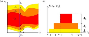
Indeed, under additional assumptions, the description of the waterbag contours evolution in time can be dramatically simplified. We assume now that each waterbag boundary can be split into pairs of non-crossing branches (figure 2
a) for which the parallel velocity can be expressed as a single-valued function of space
 $v_{\Vert }=v_{j}(x)$
. Under this assumption, the characteristic function of
 $\unicode[STIX]{x1D6FA}$
defining the waterbag volume reduces to a gate function in velocity, whose bounds are space dependent scalar fields
 $v_{j}(t,x)$
and the full multi-waterbag distribution a weighted sum of such gate functions (figure 2
b). Provided the so-called contours
 $v_{j}$
(i) do not cross, (ii) remain single-valued during the system evolution and (iii) obey a set of decoupled hydrodynamic equations in real space (see (2.7) for the explicit form), the multi-waterbag structure is preserved and the multi-waterbag distribution is an exact solution (in the weak sense) of the Vlasov equation. The initial four-dimensional dynamics in phase space is thus reduced to a finite set of three-dimensional hydrodynamic equations, which can be treated using standard Eulerian methods. The linear dynamics of the scalar fields describing the waterbag contours can be approached using perturbation around the equilibrium fields. Moreover, Fourier analysis can be applied to solve toroidal Fourier modes independently, reducing the problem to two dimensions in space.
Three bags multi-waterbag decomposition; non-crossing contours in phase space (a) and corresponding local velocity distribution at position
 $x_{0}$
(b).

2.1 Ion dynamics
The ion gyrocentre distribution function is modelled as a multi-beam distribution in the perpendicular velocity space and a multi-waterbag distribution function in parallel velocity, reading
 $$\begin{eqnarray}f(t,\boldsymbol{r},v_{\Vert },\unicode[STIX]{x1D707})=\mathop{\sum }_{\substack{ j=-N \\ j\neq 0}}^{N}\mathop{\sum }_{l=1}^{N_{\unicode[STIX]{x1D707}}}A_{jl}{\mathcal{H}}(v_{jl}(t,\boldsymbol{r})-v_{\Vert })\unicode[STIX]{x1D6FF}(\unicode[STIX]{x1D707}-\unicode[STIX]{x1D707}_{l}),\end{eqnarray}$$
where
 ${\mathcal{H}}$
is the Heaviside function. An algebraic convention is used for the waterbag index
 $j$
implying for the weights
 $$\begin{eqnarray}\forall (l,j),\quad \left\{\begin{array}{@{}l@{}}j>0\Rightarrow A_{jl}>0\\ A_{-j,l}=-A_{j,l}.\end{array}\right.\end{eqnarray}$$
In the following, summations shortened as
 $\sum _{j,l}$
shall be considered by default as taken on the whole index ranges
 ${\mathcal{I}}_{b}=[-N,-1]\cup [1,N]$
and
 ${\mathcal{I}}_{\unicode[STIX]{x1D707}}=[1,N_{\unicode[STIX]{x1D707}}]$
. The waterbag contours time evolution is governed by the transport equations
 $$\begin{eqnarray}\unicode[STIX]{x2202}_{t}v_{jl}+\boldsymbol{V}_{jl}^{GC}\boldsymbol{\cdot }\unicode[STIX]{x1D735}v_{jl}=\left(\frac{\text{d}v_{\Vert }}{\text{d}t}\right)_{jl},\quad \forall (j,l)\in {\mathcal{I}}_{b}\times {\mathcal{I}}_{\unicode[STIX]{x1D707}},\end{eqnarray}$$
where the drift velocity advection field reads
 $$\begin{eqnarray}\boldsymbol{V}_{jl}^{GC}=\frac{1}{{\mathcal{F}}_{tj\unicode[STIX]{x1D707}}}\left[v_{jl}\boldsymbol{b}+\frac{v_{jl}^{2}}{\unicode[STIX]{x1D6FA}_{CI}}\unicode[STIX]{x1D735}\times \boldsymbol{b}+\boldsymbol{b}\times \left(\unicode[STIX]{x1D707}_{l}\frac{\unicode[STIX]{x1D735}B}{B}+\frac{q_{i}\unicode[STIX]{x1D735}{\mathcal{J}}_{\unicode[STIX]{x1D707}_{l}}\unicode[STIX]{x1D719}}{B}\right)\right],\end{eqnarray}$$
and the parallel acceleration field
 $$\begin{eqnarray}\left(\frac{\text{d}v_{\Vert }}{\text{d}t}\right)_{jl}=\frac{-1}{{\mathcal{F}}_{tjl}}\left(\boldsymbol{b}+\frac{v_{jl}}{\unicode[STIX]{x1D6FA}_{CI}}\unicode[STIX]{x1D735}\times \boldsymbol{b}\right)\boldsymbol{\cdot }\left(\frac{\unicode[STIX]{x1D707}}{m_{i}}\unicode[STIX]{x1D735}B+\frac{q_{i}}{m_{i}}\unicode[STIX]{x1D735}{\mathcal{J}}_{\unicode[STIX]{x1D707}_{l}}\unicode[STIX]{x1D719}\right),\end{eqnarray}$$
with
 $$\begin{eqnarray}{\mathcal{F}}_{tjl}=1+\frac{v_{jl}}{\unicode[STIX]{x1D6FA}_{CI}}\boldsymbol{b}\boldsymbol{\cdot }\unicode[STIX]{x1D735}\times \boldsymbol{b}\approx 1.\end{eqnarray}$$
In the magnetic configuration considered here, the latter term is close to unity. Though necessary to ensure proper conservation properties of the model in nonlinear simulations, its departure from unity entails only minor frequency alterations for linear analysis, and its effects are negligible.
2.2 Electron dynamics and quasi-neutrality
The electron response follows a Boltzmann law. The strongly magnetized electrons are assumed to stay confined to magnetic surfaces, and their low inertia allows for a fast response to electrostatic potential variations, considered in this regard as ‘adiabatic’. The electron density thus reads
 $$\begin{eqnarray}n_{e}(t,\boldsymbol{r})=n_{e0}(r)\exp \left[\frac{e(\unicode[STIX]{x1D719}-\langle \unicode[STIX]{x1D719}\rangle _{FS})}{k_{B}T_{e}(r)}\right]\approx n_{e0}(r)\left(1-\left[\frac{e(\unicode[STIX]{x1D719}-\langle \unicode[STIX]{x1D719}\rangle _{FS})}{k_{B}T_{e}(r)}\right]\right),\end{eqnarray}$$
where
 $n_{e0}(r)$
,
 $T_{e0}(r)$
are prescribed profiles,
 $\langle \unicode[STIX]{x1D719}\rangle _{FS}$
is the flux surface-averaged potential, whose presence marks the fact that no screening can occur across distinct magnetic surfaces. The so-called ‘adiabatic’ electron response relies on the assumption of a strong time scale separation between the electron and potential dynamics. In the magnetic configuration considered, this assumption can be broken for the fraction of the electron population that is trapped by magnetic field intensity variations. This coupling of trapped electrons with ions leads to a substantial modification of the ITG spectral properties (see e.g. Rewoldt, Lin & Idomura Reference Rewoldt, Lin and Idomura2007; Howard et al.
Reference Howard, White, Reinke, Greenwald, Holland, Candy and Walk2013; Happel et al.
Reference Happel, Navarro, Conway, Angioni, Bernert, Dunne, Fable, Geiger, Görler and Jenko2015; Qi et al.
Reference Qi, Kwon, Hahm and Jo2016; Nakata et al.
Reference Nakata, Honda, Yoshida, Urano, Nunami, Maeyama, Watanabe and Sugama2016). Most notably the growth rate of ITG modes is significantly increased. In all the following the effect of trapped electrons will be neglected in order to keep the model simple.
The closure of the system is provided by the quasi-neutrality condition
 $n_{e}\approx n_{i}$
with the linearized polarization drift correction for the ion density, leading to
 $$\begin{eqnarray}-\unicode[STIX]{x1D735}_{\bot }\boldsymbol{\cdot }\left(\frac{n_{0}}{B\unicode[STIX]{x1D6FA}_{CI}}\unicode[STIX]{x1D735}_{\bot }\unicode[STIX]{x1D719}\right)+\frac{n_{0}e}{k_{B}T_{e}}(\unicode[STIX]{x1D719}-\langle \unicode[STIX]{x1D719}\rangle _{FS})=Z_{i}\int \text{d}^{3}v{\mathcal{J}}_{\unicode[STIX]{x1D707}}f-n_{0},\end{eqnarray}$$
where the electron adiabatic response has been linearized.
2.3 Magnetic configuration and normalization convention
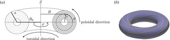
The confining magnetic field axisymmetric configuration considered here is the so-called ‘circular’ one: flux surfaces are nested tori (figure 3
b) with centred circular cross-sections. In toroidal coordinates
 $(r,\unicode[STIX]{x1D717},\unicode[STIX]{x1D711})$
(figure 3
a), in the domain defined by
 $(\unicode[STIX]{x1D717},\unicode[STIX]{x1D711})\in [0;2\unicode[STIX]{x03C0}]^{2}$
,
 $r_{min}<r<a$
, the magnetic field reads
 $$\begin{eqnarray}\boldsymbol{B}=B(b_{\unicode[STIX]{x1D717}}\boldsymbol{e}_{\unicode[STIX]{x1D717}}+b_{\unicode[STIX]{x1D711}}\boldsymbol{e}_{\unicode[STIX]{x1D711}})=\frac{B_{0}R_{0}}{R}\left(\frac{r}{qR}\boldsymbol{e}_{\unicode[STIX]{x1D717}}+\boldsymbol{e}_{\unicode[STIX]{x1D711}}\right),\end{eqnarray}$$
where
 $R=R_{0}+r\cos \unicode[STIX]{x1D717}$
and
 $(R_{0},a)$
are respectively the major and minor radius of the torus. Parameter
 $q(r)$
is the security factor and
 $s(r)=rd_{r}\ln q$
the magnetic shear. Radial dependency of the security factor is a parabolic one
 $q=q_{0}+q_{2}(r/a)^{2}$
, with
 $q_{2}>0$
so that
 $q$
is strictly monotonic. Throughout the text, radial dependencies shall be expressed using either
 $r$
,
 $x=r/a$
or
 $q$
. With this particular field configuration we have notably
 $\unicode[STIX]{x1D735}B/B=(1/R)(\cos \unicode[STIX]{x1D717}\boldsymbol{e}_{r}-\sin \unicode[STIX]{x1D717}\boldsymbol{e}_{\unicode[STIX]{x1D717}})$
,
 $\boldsymbol{b}\times (\unicode[STIX]{x1D735}B/B)=(-b_{\unicode[STIX]{x1D711}}/R)(\sin \unicode[STIX]{x1D717}\boldsymbol{e}_{r}+\cos \unicode[STIX]{x1D717}\boldsymbol{e}_{\unicode[STIX]{x1D717}})$
and
 $\unicode[STIX]{x1D735}\times \boldsymbol{b}=(b_{\unicode[STIX]{x1D711}}/R)(-\sin \unicode[STIX]{x1D717}\boldsymbol{e}_{r}-\cos \unicode[STIX]{x1D717}\boldsymbol{e}_{\unicode[STIX]{x1D717}}+((3-2s)/q)\boldsymbol{e}_{\unicode[STIX]{x1D711}})$
, up to second order in
 $\unicode[STIX]{x1D716}_{r}=r/R_{0}$
.
Toroidal geometry; toroidal coordinates (a); winding of a magnetic field line (yellow) on a rational (
 $q\in \mathbb{Q}$
) flux surface (purple) (b).

As shown in Lapillonne et al. (Reference Lapillonne, Brunner, Dannert, Jolliet, Marinoni, Villard, Görler, Jenko and Merz2009), the slight differences in magnetic geometry between this circular concentric model (dubbed as ‘ad hoc’ in Lapillonne et al. (Reference Lapillonne, Brunner, Dannert, Jolliet, Marinoni, Villard, Görler, Jenko and Merz2009)) and the
 $s{-}\unicode[STIX]{x1D6FC}$
model used in some flux-tube-based codes can lead to significant differences in both linear and nonlinear simulation results, due to inconsistencies in the
 $s{-}\unicode[STIX]{x1D6FC}$
geometry. The effects of those inconsistencies vanish in the large aspect ratio limit, and codes using consistent geometry but a different scheme yield comparable results (McMillan et al.
Reference McMillan, Lapillonne, Brunner, Villard, Jolliet, Bottino, Görler and Jenko2010).
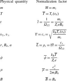
From now on, all physical quantities will be normalized using the reference values given in table 1. In this normalized system the waterbag equilibrium contours scale as
 $v_{jl}\sim O(1)$
(a few units) and their perpendicular gradients as
 $|\unicode[STIX]{x2202}_{r}\ln v_{jl}|$
,
 $|r^{-1}\unicode[STIX]{x2202}_{\unicode[STIX]{x1D703}}\ln v_{jl}|\sim \unicode[STIX]{x1D70C}_{s}/a=\unicode[STIX]{x1D70C}^{\star }\sim 10^{-2}$
. The characteristic length of the equilibrium magnetic field variations scales as
 $1/R=\unicode[STIX]{x1D70C}^{\star }\unicode[STIX]{x1D716}_{a}/(1+x\unicode[STIX]{x1D716}_{a}\cos \unicode[STIX]{x1D717})\sim \unicode[STIX]{x1D70C}^{\star }\unicode[STIX]{x1D716}_{a}\sim 10^{-3}$
.
Normalization conventions.

2.4 Equilibrium distribution function
The equilibrium distribution function used as a reference is a local Maxwellian
 $$\begin{eqnarray}f^{loc}(r,\unicode[STIX]{x1D717},v_{\Vert },\unicode[STIX]{x1D707})=\frac{n(r)}{(2\unicode[STIX]{x03C0}T(r))^{3/2}}\exp \left(-\frac{v_{\Vert }^{2}/2+\unicode[STIX]{x1D707}B(r,\unicode[STIX]{x1D717})}{T(r)}\right),\end{eqnarray}$$
where
 $n(r),T(r)$
are prescribed density and temperature radial profiles, and no equilibrium electrostatic field is present. This distribution is not a true stationary solution of the gyrokinetic Vlasov equation: a local thermodynamic equilibrium is assumed to be reached on each flux surface, which implies neglecting the radial excursion of equilibrium trajectories from said surfaces stemming from the curvature and intensity gradient of the magnetic field. In quasi-linear and nonlinear simulations this kind of initial condition entails the rapid growth of large radial electric field and consequently large scale
 $\boldsymbol{E}\times \boldsymbol{B}$
flows which prevent the onset of the instability. The so-called canonical Maxwellian, function of the true motion invariants of equilibrium characteristics, energy
 $E$
and toroidal momentum
 $P_{\unicode[STIX]{x1D711}}$
, is preferred in those cases (Idomura, Tokuda & Kishimoto Reference Idomura, Tokuda and Kishimoto2003; Dif-Praladier et al.
Reference Dif-Praladier, Grangirard, Sarazin, Garbet and Ghendrih2008). For linear analysis however, as the
 $(\unicode[STIX]{x1D717},\unicode[STIX]{x1D711})$
-averaged potential is constant and set to zero, the non-stationarity of the local Maxwellian results only in corrections on the spectral characteristics of the unstable modes (Idomura et al.
Reference Idomura, Tokuda and Kishimoto2003).
Building a multi-waterbag distribution of the form (2.5) in order to match as closely as possible the physical equilibrium corresponding to the local Maxwellian is not a trivial problem. Two methods have been used to perform this task, each having its pros and cons.
2.4.1 Maxwellian iso-surfaces methods
This method relies on the fact that in the ‘continuum’ limit in velocity space, i.e. when the number of bags and values of
 $\unicode[STIX]{x1D707}$
goes to infinity, waterbag equilibrium contours should tend to idenepsy with iso-value surfaces of the local Maxwellian. (Here we obviously assume a bounded support for both reference and multi-waterbag distributions in velocity space.) Starting from a reference point
 $(r_{0},\unicode[STIX]{x1D717}_{0},v_{0},\unicode[STIX]{x1D707})$
, the parallel velocity can be expressed as a function of
 $(r,\unicode[STIX]{x1D717})$
on the corresponding iso-surface as
 $$\begin{eqnarray}v_{\Vert }=\pm \sqrt{{\mathcal{V}}_{0}(r)^{2}+2\unicode[STIX]{x1D707}(B(r,\unicode[STIX]{x1D717}_{0})-B(r,\unicode[STIX]{x1D717}))},\end{eqnarray}$$
where
 $$\begin{eqnarray}{\mathcal{V}}_{0}^{2}(r)=v_{0}^{2}+2T\ln \left[\frac{n(r)}{n(r_{0})}\left(\frac{T(r_{0})}{T(r)}\right)^{3/2}\right]+2\unicode[STIX]{x1D707}\left[B(r_{0},\unicode[STIX]{x1D717}_{0})\frac{T(r)}{T(r_{0})}-B(r,\unicode[STIX]{x1D717}_{0})\right],\end{eqnarray}$$
provided the domain in
 $(r,\unicode[STIX]{x1D717})$
is restricted so as to ensure all quantities are real and finite. The two solution branches of (2.15) lead, for a given
 $(r_{0},\unicode[STIX]{x1D717}_{0},v_{j0}^{2},\unicode[STIX]{x1D707}_{l})$
, to a pair of symmetric contours
 $v_{\pm jl}$
. If the argument of the square root of (2.15) stays positive on the whole
 $(r,\unicode[STIX]{x1D717})$
domain, both branches stay distinct everywhere, and the contour pair is considered as ‘open’ from a topological point of view. For some values of the parameters
 $(r_{0},\unicode[STIX]{x1D717}_{0},v_{j0}^{2},\unicode[STIX]{x1D707}_{l})$
however, cancellation of the parallel velocity can occur, leading to a merging of the two branches at
 $v_{\Vert }=0$
and ‘closed’ topology for the contour pair. This closing phenomenon is slightly different whether one considers poloidal or radial variations of the parallel velocity:
-
(i) at constant
 $r$
, i.e. on a flux surface, parallel velocity variations stem directly from energy
$E=v_{\Vert }^{2}/2+\unicode[STIX]{x1D707}B$
conservation on said surface. The poloidal variations of magnetic field intensity entail the presence of a magnetic well, leading to possible poloidal trapping effects. The closing of the contour pair is then formally related to the existence of a zero-width ‘banana’ orbit on the flux surface;
-
(ii) at constant
$\unicode[STIX]{x1D703}$
the situation is more intricate: parallel velocity variations arise both from
$B$
variations and
$(n,T)$
equilibrium profiles, i.e. on the underlying radial force balance. It must be noted in particular that parallel velocity cancellation can occur even in the case of a constant magnetic field. In that case, radial variations of the Maxwellian prefactor
$nT^{-3/2}$
are sufficient to allow for contour closing.


In all cases, the presence of closed or ‘critical’ equilibrium contours has a major impact on the dynamics of the model: when two contours
 $v_{\pm jl}$
merge at some point in space, both poloidal and radial gradients diverge. This entails a divergence in the transport equation (2.7) and a coupling of the contour transport equations at the singularity points. For a linear stability analysis such as we propose here, the localization of these singularities is fixed by the setting of the equilibrium contours, so that the difficult problem of topology evolution (i.e. dynamical merging or splitting) does not have to be tackled.
Having devised a procedure to obtain equilibrium contours from the local Maxwellian iso-surface, we must now set the distribution weights
 $A_{jl}$
. They can be approximated using a mixed product quadrature rule in
 $v_{\Vert }$
(trapezoidal) and
 $\unicode[STIX]{x1D707}$
(rectangle) reading
 $$\begin{eqnarray}A_{jl}=w_{l}f^{loc}(r_{0},\unicode[STIX]{x1D717}_{0},v_{jl}+\unicode[STIX]{x0394}v/2,\unicode[STIX]{x1D707}_{l})-f^{loc}(r_{0},\unicode[STIX]{x1D717}_{0},v_{jl}-\unicode[STIX]{x0394}v/2,\unicode[STIX]{x1D707}_{l}),\end{eqnarray}$$
where
 $\unicode[STIX]{x1D6E5}_{v}=|v_{j+1l}(r_{0},\unicode[STIX]{x1D717}_{0})-v_{jl}(r_{0},\unicode[STIX]{x1D717}_{0})|$
in the case of a uniform sampling of the reference parallel velocity contours at
 $(r_{0},\unicode[STIX]{x1D717}_{0})$
, and
 $w_{l}=1/2$
for
 $l\in \{1,N_{\unicode[STIX]{x1D707}}\}$
and
 $w_{l}=1$
in other cases.
2.4.2 Moment method
Let us first consider the stationarity condition for the waterbag contours. Setting
 $\unicode[STIX]{x2202}_{t}v_{jl}=0$
in (2.7) and expressing the various fields we obtain for each axisymmetric contour
 $v_{jl}(r,\unicode[STIX]{x1D717})$
the condition
 $$\begin{eqnarray}\underbrace{\frac{1}{q}\unicode[STIX]{x2202}_{\unicode[STIX]{x1D717}}\left(\frac{v_{jl}^{2}}{2}+\unicode[STIX]{x1D707}_{l}B\right)}_{O(1)}-\underbrace{\left(\unicode[STIX]{x1D707}_{l}+\frac{v_{jl}^{2}}{B}\right)\left(\sin \unicode[STIX]{x1D717}\unicode[STIX]{x2202}_{r}v_{jl}+\frac{\cos \unicode[STIX]{x1D717}}{r}\unicode[STIX]{x2202}_{\unicode[STIX]{x1D717}}v_{jl}\right)}_{O(\unicode[STIX]{x1D70C}^{\star }\approx 10^{-2})}=0,\end{eqnarray}$$
where we have neglected the term
 $\unicode[STIX]{x1D707}(\unicode[STIX]{x1D735}\times \boldsymbol{b})\boldsymbol{\cdot }\unicode[STIX]{x1D735}B/B\ll 1$
, which is negligible in the considered low
 $\unicode[STIX]{x1D6FD}$
configuration. Taking into account the ordering of the two terms of (2.18) (coming from the
 $1/a$
scaling of equilibrium radial gradient lengths), we can first consider an approximate stationarity condition
 $$\begin{eqnarray}\unicode[STIX]{x2202}_{\unicode[STIX]{x1D717}}\left(\frac{v_{jl}^{2}}{2}+\unicode[STIX]{x1D707}_{l}B\right)=0,\end{eqnarray}$$
which is related to the conservation of energy at equilibrium on each flux surface, as the radial excursion of equilibrium trajectories from such surfaces is neglected. Assuming that, at a reference angle
 $\unicode[STIX]{x1D717}_{0}$
the radial profile
 $v_{jl}(r,\unicode[STIX]{x1D717}_{0})$
is known, (2.19) can be integrated to obtain
 $$\begin{eqnarray}v_{jl}(r,\unicode[STIX]{x1D717})=\pm \sqrt{v_{jl}(r,\unicode[STIX]{x1D717}_{0})^{2}+2\unicode[STIX]{x1D707}_{l}(B(r,\unicode[STIX]{x1D717}_{0})-B(r,\unicode[STIX]{x1D717}))},\end{eqnarray}$$
provided the square root argument is positive. As was the case for the iso-value surfaces of the local Maxwellian, (2.20) may lead to contour cancellation depending on the reference contour value
 $v_{jl}(r,\unicode[STIX]{x1D717}_{0})$
and magnetic field variation range through the choice of
 $\unicode[STIX]{x1D717}_{0}$
. It must be noted that
 $\unicode[STIX]{x1D717}_{0}$
can be set independently for each contour pair
 $v_{\pm jl}$
. In order to make use of (2.20) we must build appropriate radial profiles for the reference contours at
 $\unicode[STIX]{x1D717}_{0}$
.
In Coulette & Besse (Reference Coulette and Besse2013a
,Reference Coulette and Besse
b
), an accurate method was developed in cylindrical geometry to obtain radial profiles of equilibrium contours by equating the parallel velocity moments of the multi-waterbag distribution function and the local Maxwellian. Extension of the method to full moment equivalence for both parallel and perpendicular velocity moments gives rise to a severely ill-conditioned problem. A more tractable problem can be obtained by restricting moment equivalence to the zeroth order in
 $\unicode[STIX]{x1D707}$
(or equivalently
 $v_{\bot }$
) and putting the weights
 $A_{jl}$
in separable form
 $A_{lj}=A_{j}A_{l}$
with
 $\sum _{l}A_{l}=1$
. The
 $\unicode[STIX]{x1D707}$
weights
 $A_{l}$
are obtained as before from a rectangle quadrature rule at some reference position
 $(r_{0},\unicode[STIX]{x1D717}_{0})$
 $$\begin{eqnarray}A_{l}=\frac{\exp (-\unicode[STIX]{x1D707}_{l}B(r_{0},\unicode[STIX]{x1D717}_{0})/T(r_{0}))}{\displaystyle \mathop{\sum }_{l^{\prime }}\exp (-\unicode[STIX]{x1D707}_{l^{\prime }}B(r_{0},\unicode[STIX]{x1D717}_{0})/T(r_{0}))}.\end{eqnarray}$$
Choosing now both a common reference angle
 $\unicode[STIX]{x1D717}_{0}$
for all contours and common initial contours
 $v_{j}(r_{0},\unicode[STIX]{x1D717}_{0})$
for all
 $l$
values, the
 $2p$
th-order parallel velocity and zeroth-order
 $\unicode[STIX]{x1D707}$
moment of the multi-waterbag distribution function reads
 $$\begin{eqnarray}{\mathcal{M}}_{2p}^{MWB}=\underbrace{\mathop{\sum }_{l}A_{l}}_{=1}\mathop{\sum }_{j}A_{j}\frac{v_{j}(r_{0},\unicode[STIX]{x1D717}_{0})^{2p+1}}{2p+1}.\end{eqnarray}$$
Equating those moments with the local Maxwellian ones of same order in
 $v_{\Vert }$
and
 $\unicode[STIX]{x1D707}$
we obtain a moment equivalence problem on the sole parallel velocity moments, which can be solved for both weights and contours using the procedure described in Coulette & Besse (Reference Coulette and Besse2013b
). Although the procedure is straightforward, it must be noted that by restricting moment equivalence to the lowest moment order in
 $v_{\bot }$
, we limit by construction the accuracy of the higher-order perpendicular velocity moments. Particularly the effective perpendicular ‘temperature’
 $$\begin{eqnarray}T_{\bot }^{MWB}(r,\unicode[STIX]{x1D717})=\frac{\displaystyle \mathop{\sum }_{l}A_{l}\unicode[STIX]{x1D707}_{l}B(r,\unicode[STIX]{x1D717})\displaystyle \mathop{\sum }_{j=1}^{N}A_{j}v_{j\unicode[STIX]{x1D707}_{l}}(r,\unicode[STIX]{x1D717})}{\displaystyle \mathop{\sum }_{l}A_{l}\displaystyle \mathop{\sum }_{j=1}^{N}A_{j}v_{j\unicode[STIX]{x1D707}_{l}(r,\unicode[STIX]{x1D717})}}\end{eqnarray}$$
cannot be prescribed to equate
 $T_{0}(r)$
or even depend solely on
 $r$
with finite
 $N$
and
 $N_{\unicode[STIX]{x1D707}}$
(in the continuum limit one recovers
 $T_{\bot }=T_{\Vert }=T_{0}(r)$
). Most of the numerical results shown hereafter will be restricted to null or small values of
 $\unicode[STIX]{x1D707}$
and consequently of
 $T_{\bot }^{MWB}$
.
3 Linear analysis
We will now develop a perturbation analysis of the model. This analysis will be conducted in a first stage in a global geometric set-up. In a second stage we consider an asymptotic approach in the so-called ‘ballooning’ representation. The rationale for developing both approaches is the possibility of cross-validation of the numerical schemes within the waterbag framework. This is a necessary step before comparing with results of standard kinetic codes (whether global or ‘flux-tube’ ones) which might differ from our model in both the geometrical set-up and distribution function representation.
3.1 Two-dimensional linear problem
Decomposing the waterbag contours in their equilibrium part
 $v_{jl}(r,\unicode[STIX]{x1D717})$
and an asymptotically vanishing perturbation
 $w_{jl}(t,r,\unicode[STIX]{x1D717},\unicode[STIX]{x1D711})$
, (2.7) becomes at first order
 $$\begin{eqnarray}[{\mathcal{F}}_{jl}^{t}\unicode[STIX]{x2202}_{t}+{\mathcal{F}}_{jl}\boldsymbol{\cdot }\unicode[STIX]{x1D735}+{\mathcal{F}}_{jl}^{0}]w_{jl}+{\mathcal{G}}_{jl}\boldsymbol{\cdot }\unicode[STIX]{x1D735}{\mathcal{J}}_{\unicode[STIX]{x1D707}_{l}}\unicode[STIX]{x1D719}=0,\end{eqnarray}$$
with
 $$\begin{eqnarray}\displaystyle & \displaystyle {\mathcal{F}}_{jl}^{t}=1+\frac{v_{jl}}{B}\boldsymbol{b}\boldsymbol{\cdot }\unicode[STIX]{x1D735}\times \boldsymbol{b}, & \displaystyle\end{eqnarray}$$
 $$\begin{eqnarray}\displaystyle & \displaystyle {\mathcal{F}}_{jl}=v_{jl}\boldsymbol{b}+\frac{v_{jl}^{2}}{B}\unicode[STIX]{x1D735}\times \boldsymbol{b}+\unicode[STIX]{x1D707}_{l}\boldsymbol{b}\times \frac{\unicode[STIX]{x1D735}B}{B}, & \displaystyle\end{eqnarray}$$
 $$\begin{eqnarray}\displaystyle & \displaystyle {\mathcal{F}}_{jl}^{0}=\left[\boldsymbol{b}+\frac{2v_{jl}}{B}\unicode[STIX]{x1D735}\times \boldsymbol{b}\right]\boldsymbol{\cdot }\unicode[STIX]{x1D735}v_{jl}, & \displaystyle\end{eqnarray}$$
 $$\begin{eqnarray}\displaystyle & \displaystyle {\mathcal{G}}_{jl}=\frac{v_{jl}}{B}\unicode[STIX]{x1D735}\times \boldsymbol{b}-\frac{\boldsymbol{b}\times \unicode[STIX]{x1D735}v_{jl}}{B}. & \displaystyle\end{eqnarray}$$
Explicating the various scalar components of the vector fields we obtain
 $$\begin{eqnarray}[{\mathcal{F}}_{jl}^{t}\unicode[STIX]{x2202}_{t}+{\mathcal{F}}_{jl}^{x}\unicode[STIX]{x2202}_{x}+{\mathcal{F}}_{jl}^{\unicode[STIX]{x1D717}}\unicode[STIX]{x2202}_{\unicode[STIX]{x1D717}}+{\mathcal{F}}_{jl}^{\unicode[STIX]{x1D711}}\unicode[STIX]{x2202}_{\unicode[STIX]{x1D711}}+{\mathcal{F}}_{jl}^{0}]w_{jl}+[{\mathcal{G}}_{jl}^{x}\unicode[STIX]{x2202}_{x}+{\mathcal{G}}_{jl}^{\unicode[STIX]{x1D717}}\unicode[STIX]{x2202}_{\unicode[STIX]{x1D717}}+{\mathcal{G}}_{jl}^{\unicode[STIX]{x1D711}}\unicode[STIX]{x2202}_{\unicode[STIX]{x1D711}}]{\mathcal{J}}_{\unicode[STIX]{x1D707}_{l}}\unicode[STIX]{x1D719}=0.\end{eqnarray}$$
In the magnetic configuration considered here the so-called ‘Baños’ term
 ${\mathcal{F}}_{jl}^{t}$
is close to unity (due to that fact that
 $\boldsymbol{b}\boldsymbol{\cdot }\unicode[STIX]{x1D735}\times \boldsymbol{b}\sim 1/R$
we have in normalized form
 $(v_{j}/B)\boldsymbol{b}\boldsymbol{\cdot }\unicode[STIX]{x1D735}\times \boldsymbol{b}\sim (v_{j}/c_{s})(\unicode[STIX]{x1D70C}_{s}/R_{0})\sim \unicode[STIX]{x1D716}_{a}\unicode[STIX]{x1D70C}^{\star }\ll 1$
). As for linear analysis it entails only a negligible correction on the frequency, its departure from unity will be neglected further on.
Taking advantage of domain periodicity in
 $(\unicode[STIX]{x1D717},\unicode[STIX]{x1D711})$
the perturbed fields
 $X=(w_{jl},\unicode[STIX]{x1D719})$
are decomposed in Fourier series
 $$\begin{eqnarray}X(t,r,\unicode[STIX]{x1D717},\unicode[STIX]{x1D711})=\mathop{\sum }_{n}\mathop{\sum }_{m}X\substack{ n \\ m}(t,r)\exp (\text{i}(m\unicode[STIX]{x1D717}+n\unicode[STIX]{x1D711})).\end{eqnarray}$$
Using the axisymmetry of the equilibrium field, and approximating
 $\unicode[STIX]{x1D735}_{\bot }$
by
 $\unicode[STIX]{x1D735}_{r,\unicode[STIX]{x1D717}}$
in the quasi-neutrality equation, the problem becomes separated in
 $\unicode[STIX]{x1D711}$
, allowing us to treat the toroidal wavenumber
 $n$
as a parameter (i.e. Fourier modes
 $\text{e}^{\text{i}n\unicode[STIX]{x1D711}}$
are eigenmodes in the
 $\unicode[STIX]{x1D711}$
-direction). We will further on consider
 $n$
as fixed and will omit explicit indexing by
 $n$
of the various unknowns to simplify notations. Noting simply
 $w_{jl}$
the vector whose component are the various poloidal modes of the perturbed field, i.e.
 $w_{jl}=(w_{jl}\substack{ n \\ m}(t,r)),m\in [-m_{max},m_{max}]$
, we can express the initial value problem as
 $$\begin{eqnarray}\displaystyle & \displaystyle \unicode[STIX]{x2202}_{t}w_{jl}+F_{jl}w_{jl}+G_{jl}{\mathcal{J}}_{\unicode[STIX]{x1D707}_{l}}\unicode[STIX]{x1D719}=0,\quad \forall (j,l), & \displaystyle\end{eqnarray}$$
 $$\begin{eqnarray}\displaystyle & \displaystyle Q\unicode[STIX]{x1D719}=\mathop{\sum }_{jl}A_{jl}{\mathcal{J}}_{\unicode[STIX]{x1D707}_{l}}w_{jl}. & \displaystyle\end{eqnarray}$$
Through Laplace transform in time, one obtains a generalized eigenvalue problem, linear in the spectral parameter
 $\unicode[STIX]{x1D714}$
, which reads
 $$\begin{eqnarray}-\text{i}\unicode[STIX]{x1D714}w_{jl}+F_{jl}w_{jl}+G_{jl}{\mathcal{J}}_{\unicode[STIX]{x1D707}_{l}}\mathop{\sum }_{k^{\prime }l^{\prime }}A_{k^{\prime }l^{\prime }}Q^{-1}{\mathcal{J}}_{\unicode[STIX]{x1D707}_{l^{\prime }}}w_{k^{\prime }l^{\prime }}=0,\quad \forall (j,l),\end{eqnarray}$$
where the notation
 $Q^{-1}$
should be understood as formal, and does not preclude any explicit inversion of
 $Q$
. In a first stage, the solutions of (3.10) of interest are the most unstable ones, i.e. those for which the imaginary part
 $\unicode[STIX]{x1D6FE}$
of the complex frequency
 $\unicode[STIX]{x1D714}_{r}+\text{i}\unicode[STIX]{x1D6FE}$
is positive and maximal. Two approaches were considered for the numerical resolution of the problem, the first one operating directly on the two-dimensional problem and the second one using the expected geometry structure of the solutions to split the problem in a collection of more tractable ones through a Wentzel–Kramers–Brillouin (WKB)-like analysis which is presented hereafter.
3.2 WKB-like analysis or ‘ballooning’ representation method
A detailed and rigorous development of the following method can be found in Besse & Coulette (Reference Besse and Coulette2016): we will therefore only sketch here the main features of the asymptotic analysis and the description of the resulting problem relevant to its numerical resolution. The analysis is based on the idenepsication and separation of various space scales entering the problem and the expected solutions. An eigenmode
 $\tilde{\unicode[STIX]{x1D719}}_{\unicode[STIX]{x1D714}}$
for the electrostatic potential is decomposed in the so-called ballooning representation (Hastie & Taylor Reference Hastie and Taylor1981; Hazeltine, Hitchcock & Mahajan Reference Hazeltine, Hitchcock and Mahajan1981; Connor & Taylor Reference Connor and Taylor1987; Hazeltine & Newcomb Reference Hazeltine and Newcomb1990; Newcomb Reference Newcomb1990; Taylor, Wilson & Connor Reference Taylor, Wilson and Connor1996; Hazeltine & Meiss Reference Hazeltine and Meiss2003; Abdoul et al.
Reference Abdoul, Dickinson, Roach and Wilson2015) as such
 $$\begin{eqnarray}\tilde{\unicode[STIX]{x1D719}}_{\unicode[STIX]{x1D714}}(x,\unicode[STIX]{x1D702},\unicode[STIX]{x1D711})=\mathop{\sum }_{n\in \mathbb{Z}}\mathop{\sum }_{p\in \mathbb{Z}}\hat{\unicode[STIX]{x1D719}}_{n\unicode[STIX]{x1D714}}(x,\unicode[STIX]{x1D702}+2p\unicode[STIX]{x03C0},\unicode[STIX]{x1D703}_{k}(x))\exp \left(\text{i}n\left(\unicode[STIX]{x1D711}-2\unicode[STIX]{x03C0}pq+\int \text{d}q\unicode[STIX]{x1D703}_{k}\right)\right),\end{eqnarray}$$
where
 $\unicode[STIX]{x1D702}$
is the poloidal angle, acting as a curvilinear abscissa along a magnetic field line, and
 $\unicode[STIX]{x1D703}_{k}$
is the so-called ballooning angle. Solving the linear problem for a toroidal eigenmode
 $\tilde{\unicode[STIX]{x1D719}}_{n\unicode[STIX]{x1D714}}$
will thus entail finding both the slow varying envelope
 $\hat{\unicode[STIX]{x1D719}}_{n\unicode[STIX]{x1D714}}$
and the radial variation of the ballooning parameter
 $\unicode[STIX]{x1D703}_{k}$
. Taking advantage of the scale separation between the slow varying envelope and ballooning angle and the fast phase oscillations in the eikonal, an asymptotic expansion in the smallness parameter
 $\unicode[STIX]{x1D716}=(1/n)^{1/3}$
, provides as the lowest orders a scheme to solve the eigenproblem. The three stages of the scheme can be summarized as such:
-
(i) at the zeroth order,
$(x,\unicode[STIX]{x1D703}_{k})$
are considered as parameters. For each
$(x,\unicode[STIX]{x1D703}_{k})$
pair, the slow envelope
$\hat{\unicode[STIX]{x1D719}}_{n\unicode[STIX]{x1D714}}(\unicode[STIX]{x1D702})$
is solution of a one-dimensional integral eigenvalue problem. As the problem is by construction
$2\unicode[STIX]{x03C0}$
periodic in
$\unicode[STIX]{x1D703}_{k}$
, one has to solve in the parameter space
$[x_{min},x_{max}]\times [0,2\unicode[STIX]{x03C0}]$
. Considering for clarity only the most unstable solution sheet, one can then obtain a ‘local’ frequency map
$\unicode[STIX]{x1D714}_{0}(x,\unicode[STIX]{x1D703}_{k})$
and the corresponding local eigenvector map; -
(ii) at the first order, the lowest-order contribution of the ballooning parameter
$\unicode[STIX]{x1D703}_{k0}$
is assumed as a radially constant. Its value
$\unicode[STIX]{x1D703}_{k0T}$
is selected to ensure maximal radial extension for the mode and maximal range in the eigenfrequency
$\unicode[STIX]{x1D714}_{0}(x,\unicode[STIX]{x1D703}_{k0T})$
. This choice entails that the first-order correction
$\unicode[STIX]{x1D714}_{1}$
to the frequency is zero; -
(iii) at the second order, knowing
$\unicode[STIX]{x1D714}_{0}(x,\unicode[STIX]{x1D703}_{k0T})$
one obtains an one-dimensional eigenvalue problem for the global radial envelope
$A_{1}\propto \text{e}^{\text{i}n\int \text{d}q\unicode[STIX]{x1D703}_{k1}}$
and the global frequency
$\unicode[STIX]{x1D714}$
.


3.2.1 Integral eigenvalue problem, local in radius
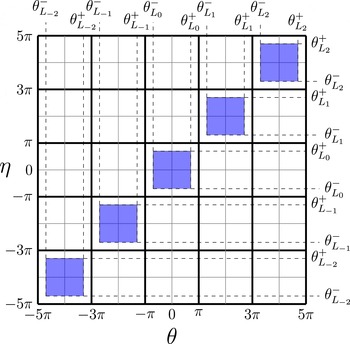
Support (blue) of a closed contour contribution in the plane
 $(\unicode[STIX]{x1D703},\unicode[STIX]{x1D702})$
; open contour contributions are defined on the whole grid.

For given values of
 $(x,\unicode[STIX]{x1D703}_{k0})$
, considered as parameters, the slow poloidal envelope
 $\hat{\unicode[STIX]{x1D719}}_{0}(\unicode[STIX]{x1D703})=\hat{\unicode[STIX]{x1D719}}_{n\unicode[STIX]{x1D714}}(x,\unicode[STIX]{x1D703},\unicode[STIX]{x1D703}_{k0})$
is the solution of the integral eigenvalue problem
 $$\begin{eqnarray}\hat{\unicode[STIX]{x1D719}}_{0}(\unicode[STIX]{x1D703})=\int _{-\infty }^{+\infty }\mathbb{K}(\unicode[STIX]{x1D703},\unicode[STIX]{x1D702},\unicode[STIX]{x1D714}_{0})\hat{\unicode[STIX]{x1D719}}_{0}(\unicode[STIX]{x1D702})\,\text{d}\unicode[STIX]{x1D702},\quad \forall \unicode[STIX]{x1D703}\in \mathbb{R},~\unicode[STIX]{x1D714}_{0}\in \mathbb{C},~\text{Im}\,\unicode[STIX]{x1D714}_{0}>0,\end{eqnarray}$$
whose integral kernel results from the individual contours contributions
 $$\begin{eqnarray}\mathbb{K}(\unicode[STIX]{x1D703},\unicode[STIX]{x1D702},\unicode[STIX]{x1D714})=\mathop{\sum }_{l}\mathop{\sum }_{j=1}^{N}\mathbb{K}_{jl}(\unicode[STIX]{x1D703},\unicode[STIX]{x1D702},\unicode[STIX]{x1D714}_{0}).\end{eqnarray}$$
The explicit form of the contour contribution
 $\mathbb{K}_{jl}$
depends on the topological nature of the corresponding equilibrium contour
 $v_{jl}$
at radial position
 $x$
. We will note respectively
 $\mathbb{K}_{jl}^{\mathit{O}}$
and
 $\mathbb{K}_{jl}^{{\mathcal{C}}}$
contributions to the kernel from an open or closed contour. The first distinction to be made between those two kinds of contributions is their support on
 $\mathbb{R}^{2}$
, which arises from the integration along equilibrium characteristics which is performed in establishing (3.12), taking boundary conditions into account. In the case of open contours, the perturbation vanishes at
 $\unicode[STIX]{x1D702}=\pm \infty$
, and the integration support is
 $\mathbb{R}^{2}$
. In the case of closed contours, the perturbation is assumed to vanish at the limit angles of the equilibrium contours. The integration procedure is then performed piecewise, for
 $p\in \mathbb{Z}$
, between limit angles
 $\unicode[STIX]{x1D703}_{Lpjl}^{-}$
and
 $\unicode[STIX]{x1D703}_{Lpjl}^{+}$
defined by
 $\unicode[STIX]{x1D703}_{Lpjl}^{\pm }=2p\unicode[STIX]{x03C0}\pm \unicode[STIX]{x1D703}_{Ljl}$
(see figure 4). A closed contour contribution is thus formally decomposed as
 $$\begin{eqnarray}\mathbb{K}_{jl}^{{\mathcal{C}}}(\unicode[STIX]{x1D703},\unicode[STIX]{x1D702})=\mathop{\sum }_{p=p_{min}}^{p_{max}}\unicode[STIX]{x1D7D9}_{]\!\unicode[STIX]{x1D703}_{Lpjl}^{-},\unicode[STIX]{x1D703}_{Lpjl}^{+}\! [}(\unicode[STIX]{x1D703})\unicode[STIX]{x1D7D9}_{]\!\unicode[STIX]{x1D703}_{Lpjl}^{-},\unicode[STIX]{x1D703}_{Lpjl}^{+}\! [}(\unicode[STIX]{x1D702})\mathbb{K}_{pjl}^{{\mathcal{C}}}(\unicode[STIX]{x1D703},\unicode[STIX]{x1D702}).\end{eqnarray}$$
In all the following explicit expressions, suitable domain restrictions will be implicitly assumed.
 $$\begin{eqnarray}\mathbb{K}_{jl}^{\mathit{O}}(\unicode[STIX]{x1D703},\unicode[STIX]{x1D702})=-\text{i}{\mathcal{P}}_{jl}(\unicode[STIX]{x1D703}){\mathcal{F}}_{jl}(\unicode[STIX]{x1D714}_{0},\unicode[STIX]{x1D702})\exp [\text{i}{\mathcal{I}}_{jl}(\min (\unicode[STIX]{x1D703},\unicode[STIX]{x1D702}),\max (\unicode[STIX]{x1D703},\unicode[STIX]{x1D702}),\unicode[STIX]{x1D714}_{0})],\end{eqnarray}$$
and
 $$\begin{eqnarray}\mathbb{K}_{pjl}^{{\mathcal{C}}}(\unicode[STIX]{x1D703},\unicode[STIX]{x1D702})={\mathcal{P}}_{jl}(\unicode[STIX]{x1D703}){\mathcal{F}}_{jl}(\unicode[STIX]{x1D714}_{0},\unicode[STIX]{x1D702})\frac{2\cos {\mathcal{I}}_{jl}(\unicode[STIX]{x1D703}_{Lpjl}^{-},\min (\unicode[STIX]{x1D703},\unicode[STIX]{x1D702}),\unicode[STIX]{x1D714}_{0})\cos {\mathcal{I}}_{jl}(\unicode[STIX]{x1D703}_{Lpjl}^{+},\max (\unicode[STIX]{x1D703},\unicode[STIX]{x1D702}),\unicode[STIX]{x1D714}_{0})}{\sin {\mathcal{I}}_{jl}(\unicode[STIX]{x1D703}_{Lpjl}^{-},\unicode[STIX]{x1D703}_{Lpjl}^{+},\unicode[STIX]{x1D714}_{0})},\end{eqnarray}$$
with the definitions
 $$\begin{eqnarray}\displaystyle & \displaystyle {\mathcal{P}}_{jl}(\unicode[STIX]{x1D703})=\frac{2\unicode[STIX]{x03C0}B(\unicode[STIX]{x1D703})}{Q(\unicode[STIX]{x1D703})}A_{jl}\frac{{\mathcal{J}}_{\unicode[STIX]{x1D707}_{l}0}(\unicode[STIX]{x1D703})}{v_{jl}(\unicode[STIX]{x1D703})}, & \displaystyle\end{eqnarray}$$
 $$\begin{eqnarray}\displaystyle & \displaystyle Q(\unicode[STIX]{x1D703})=n_{0}\left[\frac{1}{Z_{i}T_{e}}+\frac{1}{B^{2}}\left(\frac{nq\unicode[STIX]{x1D70C}_{\star }}{x}\right)^{2}(1+s^{2}(\unicode[STIX]{x1D703}-\unicode[STIX]{x1D703}_{k0})^{2})\right]+4\unicode[STIX]{x03C0}B\mathop{\sum }_{jl}A_{jl}\frac{{\mathcal{J}}_{0\unicode[STIX]{x1D707}_{l}}^{2}}{v_{jl}}, & \displaystyle\end{eqnarray}$$
 $$\begin{eqnarray}\displaystyle & \displaystyle {\mathcal{J}}_{\unicode[STIX]{x1D707}_{l}0}=J_{0}\left(\frac{|n|q\unicode[STIX]{x1D70C}_{\star }}{x}\unicode[STIX]{x1D70C}_{i}(\unicode[STIX]{x1D707}_{l})\sqrt{1+s^{2}(\unicode[STIX]{x1D703}-\unicode[STIX]{x1D703}_{k0})^{2}}\right) & \displaystyle\end{eqnarray}$$
 $$\begin{eqnarray}\displaystyle & \displaystyle {\mathcal{F}}_{jl}(\unicode[STIX]{x1D714}_{0},\unicode[STIX]{x1D702})=\frac{{\mathcal{J}}_{\unicode[STIX]{x1D707}_{l}0}(\unicode[STIX]{x1D702})}{v_{jl}(\unicode[STIX]{x1D702})}\frac{qR}{b_{\unicode[STIX]{x1D711}}}(\unicode[STIX]{x1D714}_{0}+\unicode[STIX]{x1D714}_{jl}^{\star }-\unicode[STIX]{x1D714}_{djl}+\text{i}\unicode[STIX]{x1D714}_{\diamond jl}) & \displaystyle\end{eqnarray}$$
 $$\begin{eqnarray}\displaystyle & \displaystyle \unicode[STIX]{x1D714}_{jl}^{\star }(\unicode[STIX]{x1D702})=\frac{nb_{\unicode[STIX]{x1D711}}\unicode[STIX]{x1D70C}_{\star }}{B}\left\{\frac{\unicode[STIX]{x1D70C}_{\star }}{x}[\mathfrak{q}v_{jl}\unicode[STIX]{x2202}_{x}v_{jl}-q^{\prime }(\unicode[STIX]{x1D702}-\unicode[STIX]{x1D717}_{k0})v_{jl}\unicode[STIX]{x2202}_{\unicode[STIX]{x1D702}}v_{jl}]+\left[q^{\prime }(\unicode[STIX]{x1D702}-\unicode[STIX]{x1D703}_{k0})\sin \unicode[STIX]{x1D702}+\mathfrak{q}\frac{\cos \unicode[STIX]{x1D702}}{x}\right]\frac{v_{jl}^{2}}{R}\right\}\!, & \displaystyle \nonumber\\ \displaystyle & & \displaystyle\end{eqnarray}$$
 $$\begin{eqnarray}\displaystyle & \displaystyle \unicode[STIX]{x1D714}_{djl}(\unicode[STIX]{x1D702})=\frac{nb_{\unicode[STIX]{x1D711}}\unicode[STIX]{x1D70C}_{\star }}{R}\left[\unicode[STIX]{x1D707}_{l}+\frac{v_{jl}^{2}}{B}\right]\left[q^{\prime }(\unicode[STIX]{x1D702}-\unicode[STIX]{x1D703}_{k0})\sin \unicode[STIX]{x1D702}+\mathfrak{q}\frac{\cos \unicode[STIX]{x1D702}}{x}\right]\!, & \displaystyle\end{eqnarray}$$
 $$\begin{eqnarray}\displaystyle & \displaystyle \unicode[STIX]{x1D714}_{\diamond jl}(\unicode[STIX]{x1D702})=-2\frac{b_{\unicode[STIX]{x1D711}}\unicode[STIX]{x1D70C}_{\star }v_{jl}}{RB}\left[\sin \unicode[STIX]{x1D702}\unicode[STIX]{x2202}_{x}v_{jl}-\frac{\cos \unicode[STIX]{x1D702}}{x}\unicode[STIX]{x2202}_{\unicode[STIX]{x1D702}}v_{jl}\right]\!, & \displaystyle\end{eqnarray}$$
 $$\begin{eqnarray}\displaystyle & \displaystyle {\mathcal{I}}_{jl}(\unicode[STIX]{x1D703},\unicode[STIX]{x1D702},\unicode[STIX]{x1D714}_{0})=\int _{\unicode[STIX]{x1D703}}^{\unicode[STIX]{x1D702}}\,\text{d}\tilde{\unicode[STIX]{x1D702}}\frac{qR}{b_{\unicode[STIX]{x1D711}}v_{jl}}[\unicode[STIX]{x1D714}_{0}-\unicode[STIX]{x1D714}_{djl}+\text{i}\unicode[STIX]{x1D714}_{\diamond jl}], & \displaystyle\end{eqnarray}$$
with
 $$\begin{eqnarray}\left.\begin{array}{@{}c@{}}\unicode[STIX]{x1D70C}_{\star }=a^{-1},\quad \unicode[STIX]{x1D70C}_{i}=\sqrt{{\displaystyle \frac{2\unicode[STIX]{x1D707}_{l}}{B}}},\\ \mathfrak{q}(x,\unicode[STIX]{x1D702})=q\left[1+\left({\displaystyle \frac{r}{qR}}\right)^{2}\right]=q\left[1+q^{-2}\left({\displaystyle \frac{x\unicode[STIX]{x1D716}_{a}}{1+x\unicode[STIX]{x1D716}_{a}\cos \unicode[STIX]{x1D702}}}\right)^{2}\right]\!.\end{array}\right\}\end{eqnarray}$$
3.2.2 First-order problem: selection of
$\unicode[STIX]{x1D703}_{k0T}$

The explicit structure of the integral kernel
 $\mathbb{K}$
is quite intricate. Its relevant properties will be evoked as necessary when describing the scheme and the numerical methods. For now, let us first note that the local problem is
 $2\unicode[STIX]{x03C0}$
periodic in
 $\unicode[STIX]{x1D703}_{k}$
, a property inherited from the poloidal periodicity of the equilibrium contours. We can thus restrict
 $\unicode[STIX]{x1D703}_{k0}$
values to [
 $0,2\unicode[STIX]{x03C0}$
[without loss of generality.
For a given value of
 $(x,\unicode[STIX]{x1D703}_{k0})$
, the local eigenvalue problem may have a large number of unstable (
 $\unicode[STIX]{x1D6FE}_{0}>0$
) solutions. We will consider here only the most unstable one for clarity and assume that no branch crossing arises in the parametric domain and thus that continuous solution sheets
 $(\unicode[STIX]{x1D714}_{0}(x,\unicode[STIX]{x1D703}_{k0}),\hat{\unicode[STIX]{x1D719}}(\unicode[STIX]{x1D702},x,\unicode[STIX]{x1D703}_{k0}))$
can be obtained by selecting the most unstable mode for each point in the parametric plane.
Depending on the actual magnetic field geometry and equilibrium density and temperature profiles, the local growth rate
 $\unicode[STIX]{x1D6FE}_{0}$
radial variation may not be unimodal, i.e. distinct radial unstable zones may appear. We restrict the analysis to a single such unstable zone.
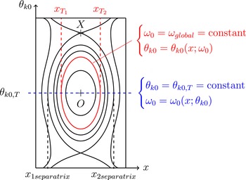
With those restrictions, the parametric variations of the frequency components have a topology similar to the ‘cat-eye’ phase space representation of an oscillator, with a single
 $O$
-point (see figure 5). Instead of considering the frequency
 $\unicode[STIX]{x1D714}_{0}$
fixed and a radially varying
 $\unicode[STIX]{x1D703}_{k}$
(in red in figure 5), the radial dependency is reported on
 $\unicode[STIX]{x1D714}_{0}$
for a fixed value
 $\unicode[STIX]{x1D703}_{k0T}$
. To ensure a maximal radial extent of the mode and avoid cutting part of the spectrum,
 $\unicode[STIX]{x1D703}_{k0T}$
is chosen as coinciding with the
 $O$
-point coordinate (dotted blue line in figure 5). This choice of the parametrization
 $\unicode[STIX]{x1D703}_{k0}=\unicode[STIX]{x1D703}_{k0T}$
,
 $\unicode[STIX]{x1D714}_{0}(x)=\unicode[STIX]{x1D714}_{0}(x,\unicode[STIX]{x1D703}_{k0T})$
entails that the first-order correction
 $\unicode[STIX]{x1D714}_{1}$
is null.
Formal representation of solutions
 $\unicode[STIX]{x1D6FE}_{0}$
,
 $\unicode[STIX]{x1D714}_{R0}=f(x,\unicode[STIX]{x1D703}_{k0})$
; level lines
 $\unicode[STIX]{x1D714}_{0}=cst$
in the vicinity of an
 $(O)$
point.

3.2.3 Second-order problem: global envelope and frequency
At the second order of the asymptotic expansion, with the choice of parametrization done at the first order, the global radial envelope
 $A_{1}\propto \text{e}^{\text{i}n\int \text{d}q\unicode[STIX]{x1D703}_{k1}}$
is solution of the Schrödinger-type one-dimensional eigenvalue problem
 $$\begin{eqnarray}\left(\frac{\unicode[STIX]{x2202}^{2}}{\unicode[STIX]{x2202}q^{2}}-n^{2}Q(\unicode[STIX]{x1D714},q)\right)A_{1}=0,\end{eqnarray}$$
with the boundary conditions
 $A_{1}(q_{min})=A_{1}(q_{max})=0$
and where the pseudo-potential
 $Q$
is defined
 $$\begin{eqnarray}Q(\unicode[STIX]{x1D714},q)=-\frac{\unicode[STIX]{x1D714}-\unicode[STIX]{x1D714}_{0}(q,\unicode[STIX]{x1D703}_{k0T})}{{\textstyle \frac{1}{2}}\unicode[STIX]{x2202}_{\unicode[STIX]{x1D703}_{k0}}^{2}\unicode[STIX]{x1D714}_{0}(q,\unicode[STIX]{x1D703}_{k0T})},\end{eqnarray}$$
and is built from the data obtained at the previous orders. The resolution of this problem yields the global mode frequency
 $\unicode[STIX]{x1D714}$
and global radial envelope
 $A_{1}(q)$
(or equivalently
 $\unicode[STIX]{x1D703}_{k1}(x)$
).
4 Numerical methods
4.1 Two-dimensional initial value problem
The unknown discrete fields of the two-dimensional problems (3.8), (3.9) or (3.10), are discretized in the radial variable on a uniform grid
 $[x_{min},x_{max}]$
. Radial differential operators are discretized using second-order centred finite difference schemes. In the poloidal variable, we use a Fourier series approach, with poloidal mode number in the spectral range
 $[m_{min},m_{max}]$
.
Let us first note that, even for the lowest ranges of reasonable discretization parameters, for instance
 $(N_{r}=100,N_{\unicode[STIX]{x1D717}}=100,N=6,N_{\unicode[STIX]{x1D707}}=6)$
, the size of the resulting operator prevents the use of a dense factorization method such as
 $QZ$
.
As we are mostly interested in the most unstable modes, a direct time integration of the initial value problem (3.8) and (3.9), from random initial conditions allows us to quickly obtain the most unstable mode for a given value of the toroidal number
 $n$
. The integration in time is performed using an explicit fourth-order explicit Runge–Kutta scheme. To ensure A-stability of the scheme, the extremal real frequencies of the spectrum are computed using the Arnoldi restarted method (Sorensen Reference Sorensen1992; Lehoucq Reference Lehoucq1996, Reference Lehoucq1999; Saad Reference Saad2001) implemented in PARPACK (Lehoucq et al.
Reference Lehoucq, Maschoff, Soresen and Yang1996).
The multi-waterbag model lends itself to straightforward parallelization over
 $N$
and
 $N_{\unicode[STIX]{x1D707}}$
of the Vlasov part of the linear system, using the MPI library. A finer grained parallelization (using OpenMP) is used for the matrix–vector products involved in computing the evolution of each contour. The overall parallel efficiency is limited by the quasi-neutrality solver, which remains sequential.
One could wonder why we do not use simply the Arnoldi method to compute the wanted unstable mode. Unfortunately, though the method converges easily when searching for extremal stable modes, we could not find any reasonable set of parameters allowing it to converge for the unstable ones. One must bear in mind that the spectrum of the operator is highly anisotropic in the complex plane, with an extent on the real axis two or three orders of magnitude larger than on the imaginary one. This may explain why the Arnoldi method, in the limited range of parameters used for tests (size of the Krylov subspace and maximal number of allowed iterations), could not converge to the desired eigenmode, as a large Krylov base and number of iterations can be necessary to filter out the unwanted high modulus eigenvalues. This lack of convergence was not extensively investigated, as the main function of the two-dimensional global code was to provide an easy to implement method to obtain most unstable modes in order to perform cross-check validation with the asymptotic eigenvalue code.
4.2 Asymptotic eigenvalue problem
4.2.1 Local integral eigenvalue problem
Problem (3.12) is a Fredholm type integral eigenvalue problem of the second kind (Kaneko & Xu Reference Kaneko and Xu1994; Rahbar & Hashemizadeh Reference Rahbar and Hashemizadeh2008) and may be discretized using several methods. Before selecting one, we first restrict the solution support in
 $\unicode[STIX]{x1D702}$
by choosing an integer
 $p_{max}$
and restricting solutions to the set
 $$\begin{eqnarray}{\mathcal{S}}=\{\hat{\unicode[STIX]{x1D719}}\in L^{2}([-2\unicode[STIX]{x03C0}p_{max},2\unicode[STIX]{x03C0}p_{max}]),\hat{\unicode[STIX]{x1D719}}(-2\unicode[STIX]{x03C0}p_{max})=\hat{\unicode[STIX]{x1D719}}(2\unicode[STIX]{x03C0}p_{max})=0\}.\end{eqnarray}$$
In order for such a restriction not to perturb the results, the actual solution must decay sufficiently fast in
 $\unicode[STIX]{x1D702}$
when
 $|\unicode[STIX]{x1D702}|\rightarrow +\infty$
so that the application of the
 $\pm \infty$
boundary conditions to finite
 $\pm 2\unicode[STIX]{x03C0}p_{max}$
has negligible impact. This property can be checked a posteriori by varying integration support. On
 $[-2\unicode[STIX]{x03C0}p_{max},2\unicode[STIX]{x03C0}p_{max}]$
, we assume a discrete grid
 $(\unicode[STIX]{x1D702}_{i},i\in [1,N_{\unicode[STIX]{x1D702}}])$
.
A first method for discretizing the integral problem is direct quadrature. Setting
 $\unicode[STIX]{x1D719}_{i}=\hat{\unicode[STIX]{x1D719}}(\unicode[STIX]{x1D702}_{i})$
we have for all
 $i\in [1,N_{\unicode[STIX]{x1D702}}]$
 $$\begin{eqnarray}\unicode[STIX]{x1D719}_{i}=\mathop{\sum }_{j}w_{j}\unicode[STIX]{x1D719}_{j}K(\unicode[STIX]{x1D702}_{i},\unicode[STIX]{x1D702}_{j},\unicode[STIX]{x1D714}_{0})=\mathop{\sum }_{j}w_{j}K_{ij}^{quad}(\unicode[STIX]{x1D714}_{0})\unicode[STIX]{x1D719}_{j},\end{eqnarray}$$
where the weights
 $w_{j}$
define a quadrature formula on nodes
 $\unicode[STIX]{x1D702}_{i}$
. Two quadrature rules where implemented: uniform grid trapezoidal and Gauss–Hermite. In both cases one obtains an eigenvalue problem of size
 $N_{\unicode[STIX]{x1D702}}$
. The direct quadrature method has the advantage of simplicity. The drawback is the coupling of quadrature accuracy and eigenvalue problem size through
 $N_{\unicode[STIX]{x1D702}}$
. In cases where
 $N_{\unicode[STIX]{x1D702}}$
is too large to allow for an efficient resolution of the eigenvalue problem, one can limit the problem size by projection of
 $\hat{\unicode[STIX]{x1D719}}$
on a function basis of size
 $N_{f}$
with
 $N_{f}<N_{\unicode[STIX]{x1D702}}$
. This projection (aka ‘Galerkin’) method was implemented with Hermite functions. The solution is thus decomposed following
 $$\begin{eqnarray}\hat{\unicode[STIX]{x1D719}}=\mathop{\sum }_{k=1}^{N_{f}}\unicode[STIX]{x1D719}_{k}\unicode[STIX]{x1D713}_{k},\quad \unicode[STIX]{x1D713}_{k}(\unicode[STIX]{x1D702})=\frac{\text{e}^{-\unicode[STIX]{x1D702}^{2}/2}}{\sqrt{2^{k}k!}}H_{k}(\unicode[STIX]{x1D702}),\end{eqnarray}$$
with
 $H_{n}$
being the
 $n$
th Hermite polynomial. The projected problem then reads, for all
 $l\in 1,\ldots ,N_{f}$
,
 $$\begin{eqnarray}\mathop{\sum }_{k}\unicode[STIX]{x1D719}_{k}\left[\underbrace{\int _{-\infty }^{+\infty }\,\text{d}\unicode[STIX]{x1D703}\unicode[STIX]{x1D713}_{l}(\unicode[STIX]{x1D703})\unicode[STIX]{x1D713}_{k}(\unicode[STIX]{x1D703})}_{D_{lk}\approx \unicode[STIX]{x1D7D9}}-\underbrace{\int _{-\infty }^{+\infty }\int _{-\infty }^{+\infty }\,\text{d}\unicode[STIX]{x1D702}\,\text{d}\unicode[STIX]{x1D703}\unicode[STIX]{x1D713}_{l}(\unicode[STIX]{x1D703})\unicode[STIX]{x1D713}_{k}(\unicode[STIX]{x1D702})\mathbb{K}(\unicode[STIX]{x1D703},\unicode[STIX]{x1D702},\unicode[STIX]{x1D714}_{0})}_{K_{lk}^{proj}(\unicode[STIX]{x1D714}_{0})}\right]=0.\end{eqnarray}$$
Assuming the use of a common quadrature method, the relation between the direct and Galerkin formulations of the problem can be expressed as
 $$\begin{eqnarray}D_{lk}=\mathop{\sum }_{i}w_{i}\unicode[STIX]{x1D713}_{li}\unicode[STIX]{x1D713}_{ki}\approx \unicode[STIX]{x1D7D9}~(\text{orthogonality}),\end{eqnarray}$$
where
 $\unicode[STIX]{x1D7D9}$
is the identity matrix, and
 $$\begin{eqnarray}K_{lk}^{proj}(\unicode[STIX]{x1D714}_{0})=\mathop{\sum }_{i}\mathop{\sum }_{j}w_{i}w_{j}\unicode[STIX]{x1D713}_{li}\unicode[STIX]{x1D713}_{kj}K_{ij}^{quad}(\unicode[STIX]{x1D714}_{0}).\end{eqnarray}$$
The choice of a fixed quadrature was made for performance reasons. For a given value of
 $\unicode[STIX]{x1D714}_{0}$
, the computation of the integral kernel at a given point
 $(\unicode[STIX]{x1D702},\unicode[STIX]{x1D703})$
has no negligible cost, and requires in particular one-dimensional quadrature computations for the
 ${\mathcal{I}}_{jl}$
integrals. With a fixed quadrature rule, one can pre-compute and store on a two-dimensional grid all the
 $\unicode[STIX]{x1D714}_{0}$
-independent elements entering the kernel. For each value of
 $\unicode[STIX]{x1D714}_{0}$
, one can then build the operator from these precomputed elements. This strategy is made mandatory by the method used for eigenvalue computation (see below), which requires building the operator for a large number of
 $\unicode[STIX]{x1D714}_{0}$
values.
Whichever of the aforementioned discretization methods is used, we obtain an eigenvalue problem of the form
 $M(\unicode[STIX]{x1D714}_{0})X=0$
, where
 $\unicode[STIX]{x1D648}$
is a square matrix whose elements depend nonlinearly on
 $\unicode[STIX]{x1D714}_{0}$
. The singularity of
 $M(\unicode[STIX]{x1D714}_{0})$
is detected using the cancellation of
 $\det (M)$
, obtained by LU factorization of
 $\unicode[STIX]{x1D648}$
. The problem is solved in two stages: the eigenvalues are sought first by solving
 $\det (M)=0$
in a region of the upper complex plane. The corresponding eigenvector is then obtained for each eigenvalue by singular value decomposition of
 $M(\unicode[STIX]{x1D714}_{0})$
.
The localization of the eigenvalues in the upper complex plane is performed using a recursive quadrisection/exclusion scheme based on contour integration: starting from a rectangle region where it is assumed no poles of
 $\det (M)$
exist, the winding number
 $N_{w}$
of
 $\det (M)$
is evaluated using Henrici’s method (see Delves & Lyness Reference Delves and Lyness1967; Davies Reference Davies1986; Kravanja & van Barel Reference Kravanja and van Barel2000; Ko, Sakkalis & Patrikalakis Reference Ko, Sakkalis and Patrikalakis2008; Zapata & Martin Reference Zapata and Martin2011 for related methods). If
 $N_{w}>1$
the region is subdivided into four slightly overlapping subregions. If
 $N_{w}=1$
, a refining procedure using the tangent method with a few starting points around the centre of the region is tested. The recursion is stopped whenever
 $N_{w}=0$
, all located roots have been found, or the maximal recursion depth is reached. Results from subregions are transmitted to their parents and siblings in order to automatically prune the search tree and avoid unnecessary computations. As is usual for root seeking schemes, the efficiency of the method has to be balanced with accuracy: though
 $\det (M)$
is known to be analytical, the convergence of Henrici’s method cannot be a priori insured for a finite number of integration points on a given contour. Calibration tests must be performed to set the maximum number of integration points so as to obtain a reasonable balance between computation cost and the risk of early termination leading to missed eigenvalues. Those tests are performed for one or a few
 $(x,\unicode[STIX]{x1D703}_{k0})$
sample values, fixing the parameters for the rest of the parametric plane, and even other
 $n$
values.
4.2.2
$\unicode[STIX]{x1D703}_{k0T}$
computation and global eigenvalue problem

The second-order (global) problem requires obtaining a good discrete representation of the mapping
 $\unicode[STIX]{x1D714}_{0}(x,\unicode[STIX]{x1D703}_{k0})$
in the parametric plane
 $(x,\unicode[STIX]{x1D703}_{k0})$
in the vicinity of the line
 $\unicode[STIX]{x1D703}_{k0}=\unicode[STIX]{x1D703}_{k0T}$
, whose value is a priori unknown. The parametric plane is first discretized on a coarse regular rectangular grid. Two acceleration strategies have been considered and implemented: on the one hand, the independence of the local eigenvalue problems corresponding to various parametric pairs
 $(x,\unicode[STIX]{x1D703}_{k0})$
lends itself to straightforward parallelization by domain decomposition in the parametric plane. With a fixed parallelization scheme, this strategy will necessarily be suboptimal as the termination times for the local searches can vary significantly in the parametric plane. On the other hand, one can exploit the continuous dependency of the kernel on
 $(x,\unicode[STIX]{x1D703}_{k0})$
. Assuming the solution
 $\unicode[STIX]{x1D714}_{0}(x,\unicode[STIX]{x1D703}_{k0})$
is known, it can be used as a guess for the solution at
 $(x+\unicode[STIX]{x1D6FF}x,\unicode[STIX]{x1D703}_{k0}+\unicode[STIX]{x1D6FF}\unicode[STIX]{x1D703}_{k0})$
. Using this guess value, the expensive recursive root locating procedure can be entirely skipped: using a few test pairs in the neighbourhood of the guess value, the solution of the problem for
 $(x+\unicode[STIX]{x1D6FF}x,\unicode[STIX]{x1D703}_{k0}+\unicode[STIX]{x1D6FF}\unicode[STIX]{x1D703}_{k0})$
can be recovered using the secant method in the complex plane.
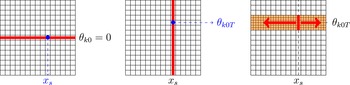
Default parametric scan scheme; parallel resolution in
 $\unicode[STIX]{x1D703}_{k0}=0$
, parallel resolution in
 $x_{s}$
, mixed resolution on a band around
 $\unicode[STIX]{x1D703}_{k0T}$
.

The default parametric scanning scheme in the implementation is a mix of both strategies (see figure 6). Moreover, two different grids are used in
 $\unicode[STIX]{x1D703}_{k0}$
in order to avoid useless oversampling: a coarse one for the localization of
 $\unicode[STIX]{x1D703}_{k0T}$
and a finer one to provide data for the global problem. We first solve the local eigenvalue problem with domain decomposition in
 $x$
with
 $\unicode[STIX]{x1D703}_{k0}=0$
. We then select the radial position
 $x_{s}$
for which the growth rate is maximal; this choice allows for a fast convergence of the root localization procedure. The problem is then solved on the line
 $x=x_{s}$
with domain decomposition in
 $\unicode[STIX]{x1D703}_{k0}$
on a coarse grid (typically
 $10^{2}$
points). Using a cubic spline approximation of
 $\unicode[STIX]{x1D714}_{0}(x_{s},\unicode[STIX]{x1D703}_{k0})$
, we then solve
 $\unicode[STIX]{x2202}_{\unicode[STIX]{x1D703}_{k0}}\unicode[STIX]{x1D714}_{0}(x_{s},\unicode[STIX]{x1D703}_{k0})=0$
for
 $\unicode[STIX]{x1D703}_{k0T}$
at
 $x=x_{s}$
. The local eigenvalue problem is then solved at
 $x=x_{s}$
, with domain decomposition in
 $\unicode[STIX]{x1D703}_{k0}$
on a thin band
 $[\unicode[STIX]{x1D703}_{k0}-\unicode[STIX]{x0394}\unicode[STIX]{x1D703}_{k0},\unicode[STIX]{x1D703}_{k0}+\unicode[STIX]{x0394}\unicode[STIX]{x1D703}_{k0}]$
around
 $\unicode[STIX]{x1D703}_{k0T}$
using a finer grid. Solutions on the whole band are then obtained by continuity in
 $x$
. The latter procedure is stopped whenever the obtained growth rate reaches negative values; the radial domain is thus restricted to
 $[x_{m},x_{M}]$
to ensure
 $\unicode[STIX]{x1D6FE}\geqslant 0$
.
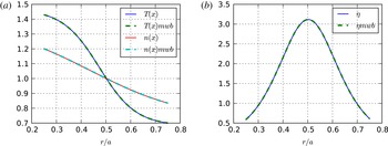
Cyclone case; prescribed (continuous lines) and multi-waterbag (dashed lines) equilibrium radial profiles; density and temperature (a);
 $\unicode[STIX]{x1D702}_{i}=L_{n}/L_{T}$
(b).

Once a discrete map
 $\unicode[STIX]{x1D714}_{0}(x,\unicode[STIX]{x1D703}_{k0})$
(and corresponding eigenvectors) have been obtained on
 $[x_{m},x_{M}]\times [\unicode[STIX]{x1D703}_{k0}-\unicode[STIX]{x0394}\unicode[STIX]{x1D703}_{k0},\unicode[STIX]{x1D703}_{k0}+\unicode[STIX]{x0394}\unicode[STIX]{x1D703}_{k0}]$
, we can build the pseudo-potential (3.27) for the global problem (3.26). The radial Laplacian is discretized using second-order centred finite differences, leading to a tridiagonal operator. The resulting eigenvalue problem is then solved using the same algorithm as the local one.
5 Sample numerical results for a Cyclone-like cases
Numerical tests have been performed with the widely used Cyclone case parameters. Based on a discharge from the Doublet-III-D tokamak, the Cyclone case is defined by the local dimensionless parameters
 $$\begin{eqnarray}\unicode[STIX]{x1D716}_{r_{0}}=\frac{r_{0}}{R_{0}}=0.18,\quad \frac{R_{0}}{L_{T}}=6.92,\quad \unicode[STIX]{x1D702}_{i}=\frac{L_{n}}{L_{T}}=3.12,\quad q=1.4,\quad s=rd_{r}\ln q=0.78,\end{eqnarray}$$
with
 $L_{X}=(d_{r}\ln X)^{-1}$
,
 $X\in \{n,T\}$
, all defined at
 $r_{0}=a/2$
. For global codes such as those depicted here, this set of local parameters is not sufficient to determine the equilibrium. As a compatible set of parameters we used for geometry
 $R_{0}=220\unicode[STIX]{x1D70C}_{s}$
,
 $a=82\unicode[STIX]{x1D70C}_{s}$
,
 $[x_{min},x_{max}]=[0.25,0.75]$
, leading to
 $\unicode[STIX]{x1D70C}_{\star }=1.22\times 10^{-2}$
and
 $\unicode[STIX]{x1D716}_{a}=0.36$
. The security factor profile is a parabolic one of the form
 $q(x)=0,854+2.184x^{2}$
. Equilibrium density and temperature are defined by radial profiles of the form
 $X(r)=\exp (\unicode[STIX]{x1D705}_{X}\unicode[STIX]{x1D6E5}_{r_{X}}\tanh ((r-r_{0})/\unicode[STIX]{x1D6E5}_{r_{X}}))$
with
 $X\in \{n,T\}$
. In all results presented here, we used
 $L_{n}=100$
,
 $\unicode[STIX]{x1D6E5}_{r_{n}}=0.4a$
,
 $L_{T}=32.1$
,
 $\unicode[STIX]{x1D6E5}_{r_{T}}=0.15a$
, yielding profiles (see figure 7) similar to those used in Idomura et al. (Reference Idomura, Tokuda and Kishimoto2003). In this section, we will first discuss shortly the choices made for multi-waterbag equilibrium building and their impact on solver behaviour. We will then present results for equilibria where both codes can operate fully, allowing for cross-comparison of the results. We will eventually discuss the case of equilibria containing closed contours, which as of now can only be treated locally in the radial variable with the asymptotic method.
5.1 Multi-waterbag equilibrium distribution building
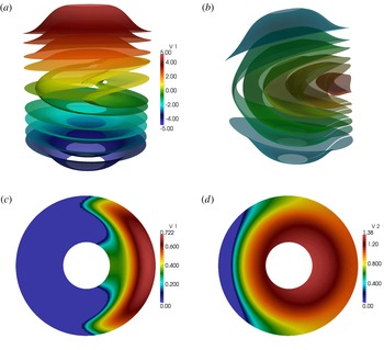
As stated in § 2.4, whatever method is used to build the equilibrium multi-waterbag contours, some contours may ‘close’ on the spatial domain whenever the magnetic moment
 $\unicode[STIX]{x1D707}$
is non-zero (see figure 8). For the latter, the divergence of the contour spatial gradients at limit angles strongly perturb the linearized advection operators. The initial value code cannot in its present state be used to tackle these cases, as the effect of those divergences cannot be filtered out. In order to be able to compare results from both codes, we have first considered equilibria where no such closed contour appear by strongly limiting the range in magnetic moment. The equilibrium contours are built using the moment equivalence method at
 $\unicode[STIX]{x1D717}=0$
.
Cyclone case with
 $N=6$
;
 $N_{\unicode[STIX]{x1D707}}=1~\unicode[STIX]{x1D707}=1$
;
 $(r,\unicode[STIX]{x1D717},v_{\Vert })$
view of equilibrium contours built with the moments method (a) and local Maxwellian iso-surfaces topology (b);
 $(r,\unicode[STIX]{x1D717})$
view of the ‘closed’
 $v_{1}$
(c) and
 $v_{2}$
(d) contours.

5.2 Results from the QUALITORO code
Table 2 displays the parameters used for the QUALITORO test runs on the Cyclone case. For all results presented here, the eigenmode characteristics are examined using the electrostatic potential. Growth rates and frequencies are both computed locally on the radial domain, at
 $x_{0}=0.5$
. Growth rates are obtained by logarithmic regression on
 $\int |\unicode[STIX]{x1D719}(t,x_{0},\unicode[STIX]{x1D717})|^{2}\,\text{d}\unicode[STIX]{x1D717}$
. Frequencies are extracted from the time Fourier spectrum of
 $\cos [\arg \unicode[STIX]{x1D719}(t,x_{0},\unicode[STIX]{x1D717}_{0}=0)]$
, computed in the linear growth phase to exclude transient frequencies.
QUALITORO initial value code parameters; time step
 $\unicode[STIX]{x0394}t$
; number of time steps
 $N_{t}$
; number of
 $n$
toroidal wavenumber values
 $N_{\unicode[STIX]{x1D711}}$
; number of MPI processes
 $N_{proc}=2\times N\times N_{\unicode[STIX]{x1D707}}+1$
; number of threads per MPI process
 $N_{thread}$
.

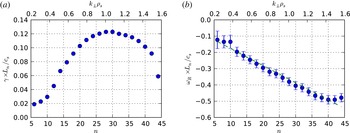
Cyclone-like case;
 $N=6$
,
 $N_{\unicode[STIX]{x1D707}}=1$
,
 $\unicode[STIX]{x1D707}=0$
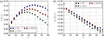
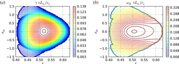
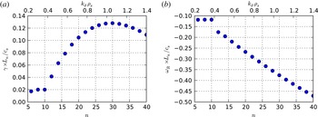
; QUALITORO code results; growth rate (a) and frequencies (b) obtained from electrostatic potential in
 $(x_{0}=0.5,\unicode[STIX]{x1D717}_{0}=0)$
.

The spectral
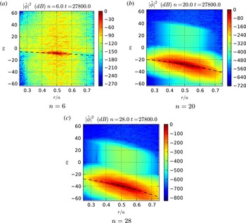
 $n$
-dependency of the growth rates and frequencies for the Cyclone case is shown on figure 9. As a comparison basis, we will consider results for the same case presented in Dimits et al. (Reference Dimits, Bateman, Beer, Cohen and Dorland2000), Grandgirard et al. (Reference Grandgirard, Sarazin, Garbet, Dif-Pradalier, Ghendrih, Crouseilles, Latu, Sonnendrücker, Besse and Bertrand2006b
), Rewoldt et al. (Reference Rewoldt, Lin and Idomura2007), Idomura et al. (Reference Idomura, Ida, Kano, Aiba and Tokuda2008), Lapillonne et al. (Reference Lapillonne, Brunner, Dannert, Jolliet, Marinoni, Villard, Görler, Jenko and Merz2009), Qi et al. (Reference Qi, Kwon, Hahm and Jo2016).
5.2.1 Case of an equilibrium distribution function with no trapped particles
$(\unicode[STIX]{x1D707}=0)$

There is only a qualitative similarity between the results in figure 9 for the
 $\unicode[STIX]{x1D707}=0$
no-trapping limit, and the reference results for the Cyclone case which are shown in figure 25(a). The real part of the frequency exhibits the same linear trend as in the reference results, and the overall range in growth rate is quite similar. There is clearly no quantitative agreement though, even for the lowest part of the spectrum where finite Larmor radius effect disappear. The discrepancy comes from the very peculiar nature of the equilibrium distribution (
 $T_{\bot }=0$
) which differs significantly from the standard (Maxwellian) Cyclone distribution function. A second possible source of discrepancy is the value of
 $\unicode[STIX]{x1D70C}^{\star }=1/82$
: it is too large to exclude possible finite domain size effects on the spectrum, which should become negligible around
 $\unicode[STIX]{x1D70C}^{\star }=1/200$
according to McMillan et al. (Reference McMillan, Lapillonne, Brunner, Villard, Jolliet, Bottino, Görler and Jenko2010).
A discontinuity in the variations of
 $\unicode[STIX]{x1D6FE}$
and
 $\unicode[STIX]{x1D714}$
is visible in the lower part of the spectrum, indicating a possible branch jump.
An important, but unsurprising difference with reference results is the support of the spectrum in
 $n$
, and consequently in
 $k_{\bot }$
, with higher peak wavenumber and range. As the equilibrium distribution in magnetic moment is limited to the
 $\unicode[STIX]{x1D707}=0$
value, the gyroaverage operator reduces to identity and the only retained finite Larmor radius effect is the polarization drift. The
 $k_{\bot }$
spectrum is thus similar to the drift-kinetic one in cylindrical geometry, with a peak around
 $k_{\bot }\unicode[STIX]{x1D70C}_{s}\sim 1$
and a slow decreasing tail at high frequencies.
The geometric features of the mode envelopes (figure 11) exhibit a variation with
 $n$
. For small wavenumbers, the mode structure is similar to the one observed for cylindrical ITG modes: a radial localization in the high gradient zone, with a narrow-banded poloidal spectrum, and a weak poloidal localization. When
 $n$
grows, the ballooning features of the mode is accentuated. The slowly varying radial envelope corresponding to the gradient zone is then modulated by the fast oscillations caused by resonant flux surfaces. A slight drift of the radial envelope peak from the maximum gradient position
 $x_{0}$
to the exterior of the torus can be also observed (figure 10). The poloidal spectrum widens, and the mode develops a slow varying poloidal envelope localized in the low field side.
The resonant character of the mode is clearly marked in the radial dependency of the poloidal Fourier spectrum of the mode (figure 12). The latter is strongly localized around the resonance curve
 $m=-nq$
.
All features observed are consistent with the ones observed in Idomura et al. (Reference Idomura, Tokuda and Kishimoto2003).
QUALITORO code; Cyclone-like case;
 $N=6$
,
 $N_{\unicode[STIX]{x1D707}}=1$
,
 $\unicode[STIX]{x1D707}=0$
; radial profiles of potential modulus in
 $\unicode[STIX]{x1D717}=0$
for a few
 $n$
values.

QUALITORO code; Cyclone case;
 $N=6$
,
 $N_{\unicode[STIX]{x1D707}}=1$
,
 $\unicode[STIX]{x1D707}=0$
; real part of electrostatic potential; poloidal cut with local Cartesian basis
 $(X=r/a\cos \unicode[STIX]{x1D717},Y=r/a\sin \unicode[STIX]{x1D717})$
.

QUALITORO code; Cyclone-like case;
 $N=6$
,
 $N_{\unicode[STIX]{x1D707}}=1$
,
 $\unicode[STIX]{x1D707}=0$
; radial dependency of poloidal Fourier power spectrum (in dB); dashed line indicates resonance
 $m=-nq(r)$
.

5.2.2 Non-zero magnetic moment effect
As stated before, avoiding the existence of closed equilibrium contours imposes a strong limit on the accessible magnetic moment range (
 $\unicode[STIX]{x1D707}_{max}=0.17$
). The introduction of non-zero magnetic moment distributions has nonetheless a noticeable effect on the spectral
 $n$
-dependencies of the instability. Toroidal number scans have been performed using three distinct distributions in magnetic moment. The first two each have one unique value of the magnetic moment, respectively
 $\unicode[STIX]{x1D707}=0$
and
 $\unicode[STIX]{x1D707}=0.15$
. The last one combines the two values. The resulting growth rates and frequencies are given on figure 13. The increase in magnetic moment modifies the spectral dependency of the growth rate in multiple ways; the higher end (
 $n>15$
) of the spectrum is stabilized, while the lower end is slightly destabilized and the maximum is shifted towards lower frequencies. The effect on frequencies is a shift of the spectrum towards low values of
 $n$
. Though limited, all the aforementioned effects show a trend which is consistent with reference results obtained with more complete equilibrium distributions. For the limited range of
 $\unicode[STIX]{x1D707}$
values used here, the global evolution of the modes geometry is not noticeably affected.
QUALITORO code; Cyclone-like case; magnetic moment dependency of growth rates (a) and frequencies (b).

5.3 Results from the ASYMPTORO code
The asymptotic method has been implemented in the ASYMPTORO code. Though both direct quadrature and Galerkin schemes were implemented and tested, we will present here only the direct quadrature results. In the case tested, the former scheme proved more costly without any significant accuracy or stability advantage. Before presenting global results suitable for comparison with the initial value code, we will first retrace the different computation steps of the asymptotic method on a few sample cases.
5.3.1 Resolution of the local eigenvalue problem in
$(x,\unicode[STIX]{x1D717}_{k0})$

Solving the integral eigenvalue problem described in § 4.2.1 first requires setting both integration bounds and resolution for the
 $\unicode[STIX]{x1D702}$
variable. The integration range, and consequently the solution support on
 $\mathbb{R}$
of the discrete solution, is defined as
 $[-(2p_{max}+1)\unicode[STIX]{x03C0},(2p_{max}+1)\unicode[STIX]{x03C0}]$
, where
 $p_{max}$
is a chosen integer. The accuracy is then fixed by the choice of
 $N_{\unicode[STIX]{x1D702}}$
. On figure 14, convergence results for the local growth rate and frequency, obtained from a scan in both
 $p_{max}$
and
 $\unicode[STIX]{x1D702}$
are shown for the
 $n=25$
mode in
 $(x=0.5,\unicode[STIX]{x1D717}_{k0}=0)$
. Below 5 % convergence in relative value is obtained for
 $h_{\unicode[STIX]{x1D702}}\sim 0.2$
.
ASYMPTORO code; Cyclone-like case;
 $n=25$
mode; convergence test in
 $(x=0.5,\unicode[STIX]{x1D717}_{k0}=0)$
;
 $p_{max}$
(shortened as
 $p$
in legends) defines the solution support (
 $[-(2p_{max}+1)\unicode[STIX]{x03C0};(2p_{max}+1)\unicode[STIX]{x03C0}]$
);
 $N_{\unicode[STIX]{x1D702}}$
scan over values 65, 129, 257, 513.

ASYMPTORO code; Cyclone-like case; local problem in
 $(x=0.5,\unicode[STIX]{x1D717}_{k0}=0)$
; most unstable solution envelopes;
 $n=25$
on
 $[-5\unicode[STIX]{x03C0};5\unicode[STIX]{x03C0}]$
(a);
 $n=10$
on
 $[-7\unicode[STIX]{x03C0};7\unicode[STIX]{x03C0}]$
(b).

For an accurate description of mode geometry, the convergence in
 $h_{\unicode[STIX]{x1D702}}$
of the eigenvalue is not sufficient, and the decrease of the solution when reaching domain boundaries must be taken into account to set
 $p_{max}$
properly. As can be seen in figure 15, the typical width of the local solution decreases with the toroidal mode number
 $n$
. For the higher part of the spectrum (typically
 $n\geqslant 15$
), setting
 $p_{max}=1$
is sufficient, while for the lower parts, extension of the solution envelope requires higher settings.
We have so far considered only the most unstable solution to the local eigenvalue problem. For most of the spectral range in
 $n$
, the growth rate of less unstable ones is orders of magnitude lower than the most unstable, and they are typically discarded by setting the solver lower threshold in
 $\unicode[STIX]{x1D6FE}$
. For the lower part of the spectrum, secondary solutions with significant growth rate may appear. This is for instance the case of the
 $n=10$
mode. This observation confirms existence of the branch jump around
 $n=10$
that was suggested when examining the initial value code results (figure 16).
ASYMPTORO code; Cyclone-like case; local problem in
 $(x=0.5,\unicode[STIX]{x1D717}_{k0}=0)$
;
 $n=10$
mode; map of argument of operator determinant in the complex plane (a); recursive solver search boxes in red with winding number in black; white crosses indicate converged solution; envelope of the second most unstable solution (b).

5.3.2 Global problem
Before attempting to compute the
 $\unicode[STIX]{x1D703}_{k0T}$
angle, one must insure that continuous solutions sheets in the parametric plane can be assembled from local results obtained independently (i.e. without using the fast continuation method). Ambiguities may arise in zones where the growth rate reaches small values, as multiple solutions with comparable growth rates coexist. In that zone marking the boundary of the unstable island in the parametric plane, the local problem becomes harder and more costly to solve as the growth rate diminishes. As these zones correspond to radial positions where the global envelope will be vanishingly small, imposing a lower cutoff threshold on the growth rate when selecting solutions does not entail significant modification of the mode structure. The chosen threshold must simply be low enough to obtain a strongly confining pseudo-potential
 $Q$
(3.27) when solving the global Schrödinger problem. Frequency maps obtained by applying such a threshold are shown on figure 17.
ASYMPTORO code; Cyclone-like case; contour plot of local frequencies
 $(\unicode[STIX]{x1D6FE},\unicode[STIX]{x1D714}_{R})$
in the parametric plane
 $(x,\unicode[STIX]{x1D703}_{k0})$
;
 $n=24$
,
 $p_{max}=2$
,
 $N_{\unicode[STIX]{x1D702}}=257$
; growth rate lower threshold
 $\unicode[STIX]{x1D6FE}_{min}\times L_{n}/c_{s}=0.016$
.

The localization of the
 $(O)$
-point and of the whole unstable zone depends on the toroidal mode number. For all cases tested so far, the value of the ballooning angle
 $\unicode[STIX]{x1D703}_{k0T}$
remains close to zero. The radial position of the
 $(O)$
point grows with
 $n$
, consistent with the observed behaviour of the mode radial envelope observed in the results of the initial value code (figure 10). With growing
 $n$
, variations of the eigenfrequencies with
 $\unicode[STIX]{x1D703}_{k0}$
become slightly more complex and the
 $\unicode[STIX]{x1D703}_{k0}$
component of the gradient of
 $\unicode[STIX]{x1D714}_{0}$
may vanish in more than one point for some values of
 $x$
(figure 18). To avoid these zones when using the fast continuation method, a first sweep in
 $x$
with
 $\unicode[STIX]{x1D703}_{k0}=0$
is done in order to obtain a good approximation of the
 $x$
-position of the
 $(O)$
point. The scan in
 $\unicode[STIX]{x1D703}_{k0}$
is then done at this position, where variations of the growth rate are unimodal in
 $\unicode[STIX]{x1D703}_{k0}$
. Once the value of
 $\unicode[STIX]{x1D703}_{k0T}$
has been obtained from such a scan, the local problem may be solved on a thin band of the domain centred on
 $\unicode[STIX]{x1D703}_{k0T}$
, in order to build the operator for the global problem. As can be seen on figure 19(a), the pseudo-potential for the Schrödinger operator is strongly confining. Though oscillations stemming from the second derivatives in the expression of
 $Q$
are visible, their impact on the actual solution is low as the envelope of the solution decays rapidly (figure 19
b).
ASYMPTORO code; Cyclone-like case;
 $n=40$
,
 $p_{max}=1$
,
 $N_{\unicode[STIX]{x1D702}}=185$
; contour plots of the local growth rate in the
 $(x,\unicode[STIX]{x1D717}_{k0})$
plane.

ASYMPTORO code; Cyclone-like case;
 $n=24$
,
 $p_{max}=2$
,
 $N_{\unicode[STIX]{x1D702}}=257$
; global radial envelope computation; radial profile of the pseudo potential
 $Q$
(a); radial profile of the solution
 $A(x)$
(b).

Once the slow radial envelope
 $A(x)$
has been obtained, the global mode is reconstructed from both
 $A(x)$
and local solutions envelopes
 $\hat{\unicode[STIX]{x1D719}}(x,\unicode[STIX]{x1D702},\unicode[STIX]{x1D703}_{k0T})$
. As the latter were obtained independently, each of them is defined up to an arbitrary unitary phase factor. A phase shift is applied in order to restore phase continuity in
 $x$
of the envelopes (figure 20). The reconstruction is obtained by
 $$\begin{eqnarray}\unicode[STIX]{x1D719}(x,\unicode[STIX]{x1D717})\sim \mathop{\sum }_{p=-p_{max}}^{p_{max}}\hat{\unicode[STIX]{x1D719}}(x,\unicode[STIX]{x1D717}+2p\unicode[STIX]{x03C0},\unicode[STIX]{x1D703}_{k0T})A(x)\text{e}^{-\text{i}nq(x)(\unicode[STIX]{x1D717}+2p\unicode[STIX]{x03C0}-\unicode[STIX]{x1D703}_{k0T})},\end{eqnarray}$$
leading to the global mode (figure 21). The dependencies in the toroidal mode number
 $n$
of the spectral and geometric features of the mode obtained by the asymptotic method are similar to those observed for the initial value code (figure 22). The discontinuity in the low end of the spectrum is confirmed. The evolution of mode geometry with
 $n$
is similar to the one observed with the initial value code; apart from the ballooning structure, which appears by construction, the radial out-shift of the radial envelope with growing
 $n$
is also observed.
ASYMPTORO code; Cyclone case;
 $n=24$
,
 $p_{max}=2$
,
 $N_{\unicode[STIX]{x1D702}}=257$
; local envelopes
 $\hat{\unicode[STIX]{x1D719}}(x,\unicode[STIX]{x1D702},\unicode[STIX]{x1D703}_{k0T})$
; modulus (a) real part (b).

ASYMPTORO code; Cyclone-like case;
 $n=24$
,
 $p_{max}=2$
,
 $N_{\unicode[STIX]{x1D702}}=257$
; global solution
 $\unicode[STIX]{x1D719}(x,\unicode[STIX]{x1D717})$
; real part (a) and modulus (b).

ASYMPTORO code; Cyclone-like case;
 $N_{\unicode[STIX]{x1D707}}=1$
,
 $\unicode[STIX]{x1D707}=0$
; variation with
 $n$
of global growth rate (a) and frequency (b).

5.4 Cross-comparisons
As the overall spectral and geometric features of the solutions obtained from both method appear to be consistent, a more direct comparison of the instability spectra is possible. Scans in toroidal number have been performed, for both methods, using a fixed set of parameters (resolution, domain, time step,
 $\ldots$
) adapted to the central part of the toroidal range (
 $n=15{-}35$
). Comparing growth rates and frequencies (figure 23
a,b) in that range reveals a good agreement between the two methods, with relative variation of about 5 %. Larger discrepancies appear for the less unstable modes at both extremities of the spectrum.
Cyclone-like case; growth rate (a) and frequency (b) comparison between initial value (continuous lines) and asymptotic method (dashed); growth rate data are interpolated by cubic splines; frequencies are interpolated by affine fit.

The geometry of the envelopes obtained by both methods also show good agreement, as can be seen (figure 24) for the
 $n=20$
mode. The poloidal and radial localization of the mode are consistent, with a slightly higher attenuation on the high field side for the asymptotic mode (figure 24
c,d).
Cyclone-like case;
 $N_{\unicode[STIX]{x1D707}}=1$
,
 $\unicode[STIX]{x1D707}=0$
;
 $n=20$
mode; real part (a,b) and modulus (c,d) of mode envelopes obtained by both methods.

5.5 Extension of the method to distributions containing closed contours
The previous results were obtained from equilibrium multi-waterbag distributions containing only ‘open’ contours, i.e. for which the non-crossing condition is everywhere valid on the domain. Such a restriction entailed a drastic limitation of the extension of the distribution in magnetic moment. Overcoming this limitation requires a proper treatment of ‘closed’ equilibrium contours. Strictly speaking the latter violate the non-crossing assumption, and the dynamics of symmetric contour pairs are coupled. The resulting singularities cannot be properly treated using the initial value solver. For the asymptotic solver, the situation is somewhat less critical. Solutions of the local eigenvalue problem can be obtained for equilibrium distributions containing closed contours as their contributions to the integral kernel
 $\mathbb{K}$
are only weakly singular in
 $\unicode[STIX]{x1D717}$
at the limit angles, and thus integrable. For equilibrium contours built using the moments method, extending the range of the distribution in magnetic moment results in an overly strong stabilization. The constraints of the moment method in its present form, and most notably the restriction of moment equivalence to the lowest order in magnetic moment, prevent a satisfactory sampling of the equilibrium. For equilibrium distributions built from Maxwellian iso-surfaces, we observe a better agreement with reference results: on figure 25(a), local growth rates and frequencies of the eigenvalue code are plotted along data extracted from Dimits et al. (Reference Dimits, Bateman, Beer, Cohen and Dorland2000), GTC/GT3D/FULL data from Rewoldt et al. (Reference Rewoldt, Lin and Idomura2007), GYSELA data from Grandgirard et al. (Reference Grandgirard, Sarazin, Garbet, Dif-Pradalier, Ghendrih, Crouseilles, Latu, Sonnendrücker, Besse and Bertrand2006b
), GS2 documentation reference Cyclone data and data computed using the eigenvalue solver of the GENE code (Jenko et al.
Reference Jenko, Dorland, Kotschenreuther and Rogers2000; Lapillonne et al.
Reference Lapillonne, Brunner, Dannert, Jolliet, Marinoni, Villard, Görler, Jenko and Merz2009; Görler et al.
Reference Görler, Lapillonne, Brunner, Dannert, Jenko, Merz and Told2011) with
 $s{-}\unicode[STIX]{x1D6FC}$
geometry. One should keep in mind when considering those results that the obtained frequencies and growth rates are the lowest-order radially local approximation of the global ones in the asymptotic expansion. The weak singularities stemming from the presence of closed contours entail nonetheless a loss of regularity of the poloidal envelope
 $\hat{\unicode[STIX]{x1D719}}$
at the limit angles (figure 25
b).
Solutions of the local eigenvalue problem in
 $x=0.5$
,
 $\unicode[STIX]{x1D703}_{k0}=0$
; equilibrium build from local Maxwellian iso-surfaces with
 $N=10$
,
 $N_{\unicode[STIX]{x1D707}}=10$
,
 $\unicode[STIX]{x1D707}_{max}=8$
with Cyclone parameters; (a) local growth rate and frequencies (red circles) with data from Dimits et al. (Reference Dimits, Bateman, Beer, Cohen and Dorland2000) (blue crosses), Rewoldt et al. (Reference Rewoldt, Lin and Idomura2007) (black stars), GYSELA data from Grandgirard et al. (Reference Grandgirard, Sarazin, Garbet, Dif-Pradalier, Ghendrih, Crouseilles, Latu, Sonnendrücker, Besse and Bertrand2006b
) (cyan x’s), GS2 data (green squares), GENE (version 11 release 1.7) data (yellow diamonds); (b) poloidal envelope
 $\hat{\unicode[STIX]{x1D719}}$
for the mode
 $n=10$
.

6 Conclusions and prospects
We presented here the first attempt at applying the multi-waterbag reduction to global linear analysis of ITG modes in toroidal geometry. We developed both an eigenvalue solver based on asymptotic expansion in the ballooning representation and an initial value solver relying on no assumptions on the geometric structure of solutions. The first tests were performed using equilibria for which both methods can operate. Results indicate (i) a qualitative agreement of the obtained solutions with known spectral and geometric properties of the instability, (ii) consistency between the two methods in a large part of the toroidal number spectral range.
The case of equilibria built with a larger support in magnetic moment can only as of now be treated locally in radius with the eigenvalue solver. The obtained local frequencies and growth rate appear to be in reasonably good agreement with reference results. This is a very encouraging result considering the low resolution in velocity space (
 $N=10,N_{\unicode[STIX]{x1D707}}=10$
) of the model and the consequent low numerical cost (the computation of the local solutions of figure 25(a) takes only approximately twenty minutes on a laptop). The impact of the inclusion of closed contours entail a divergence of the equilibrium contours spatial gradients. The resulting singularities do not prevent the resolution of the radially local eigenvalue problem, but break the continuity in radius of the operator required for a full global resolution.
Two approaches may be considered to treat those issues. The first relies on improving the equilibrium building methods in order to limit or avoid closed contours without restricting the range in magnetic moment. This requires excluding trapped particle trajectories from the equilibrium distribution, which is not straightforward in the multi-waterbag context: the spatial variation of an equilibrium contour can indeed in many cases lead to a crossing of the trapping boundary in velocity space. The second relies on developing a regularization procedure to improve the treatment of poloidal and radial singularities in the asymptotic method.
In any case, though the Eulerian formulation of the waterbag model allowed us to obtain ITG modes characteristics in reasonable agreement with other codes, it is clearly unsuited for global nonlinear simulations. The next major steps in continuation of this work will be (i) to develop a nonlinear initial value code based on the Lagrangian formulation of the waterbag model by taking advantage of the technical groundwork done in Sousbie & Colombi (Reference Sousbie and Colombi2016) and (ii) to perform a more systematic comparison of waterbag results with other global or local gyrokinetics codes.
Acknowledgements
The second author acknowledges the support of the VLASIX and EUROFUSION projects respectively under the grants nos ANR-13-MONU-0003-01 and EURATOM-WP15-ENR-01/IPP-01.