In the pre-1914 gold standard era, the American economy suffered financial crises more frequently than other countries (Bordo 1985) with all the usual symptoms: mass withdrawals of funding from financial intermediaries, choked-off credit supply, and payment system breakdowns. Economists believe America was especially vulnerable to financial crises because it had no central bank to act as lender of last resort, and its banks were not allowed to form branch networks to diversify risk. But these structural features of the financial system do not explain why a crisis occurred in one year rather than another. It is important to identify the exogenous factors that triggered pre-1914 crises, not just to complete the historical account but to advance economic research. Recent studies have used data from the pre-1914 United States (among other times and places) to identify antecedents and peculiar effects of financial crises in general (e.g., Reinhart and Rogoff 2011; Bordo and Haubrich 2010; Schularick and Taylor 2012). For such purposes, one must be able to distinguish effects of a crisis per se from the conditions that triggered it and from those conditions’ other repercussions.
Before 1914 contemporary observers believed that monetary shocks originating in agriculture caused many of America's financial crises. Rural households and businesses made relatively little use of bank accounts, so payments associated with autumn harvests and spring planting created seasonal surges of demand for cash. To accommodate them, rural banks withdrew their deposits in financial center banks, leaving the latter with low reserves of liquid assets. Thus, a further decrease in deposits or increase in loan defaults that would be shrugged off in other seasons could touch off a crisis in autumn or spring (Sprague 1910, p. 127; Kemmerer 1911, p. 48). Apart from seasonal effects on money demand, contemporaries believed year-to-year fluctuations in harvests of America's major export crops, cotton and wheat, could affect money supply and hence financial conditions through the gold standard specie-flow mechanism. America was part of the international gold standard system from January 1879, when the Treasury began to redeem currency in gold, until the First World War when most countries suspended gold convertibility. According to A. Piatt Andrew (1906, p. 326):
The size of the crops will exert a considerable influence upon the balance of trade and the international movement of gold. The extent of bank reserves in the great financial centers and the contraction or expansion of general credit may in consequence depend most importantly upon the output of the season's harvests…When the American crops are abundant, our exports very naturally tend to increase, and gold imports are apt to occur…When, on the other hand, the movement of exports and of gold swings in the contrary direction, …we are apt to be confronted with dwindling bank reserves, a contingent contraction of the general credit, declining business, and less activity in trade.
Because agricultural shocks to cash demand and export revenue were transitory, a central bank could have sterilized them by adjusting the supply of an “elastic” currency—non-gold high-powered money—without endangering the country's commitment to the gold standard. Thus, in the policy debates leading up to the foundation of the Federal Reserve, proponents of a central bank for the United States frequently invoked agricultural shocks’ purported disruptions to financial conditions (Wicker 2005).
In modern economic literature, Jeffrey A. Miron (1986) supports this old view, arguing that seasonal peaks in rural activity raised interest rates, drained bank reserves, and raised the probability of panics; that realized panics probably caused business cycle downturns; and that the creation of the Fed eased these problems. But a more common view in modern literature appears to have little role for monetary shocks originating in agriculture. Gary Gorton (1988), Jack W. Wilson, Richard E. Sylla, and Charles P. Jones (1990), Frederic S. Mishkin (1991), and Charles Calomiris and Gorton (1991) argue that pre-1914 crises were effects rather than causes of business cycle downturns: depositors withdrew en masse because they feared a recession would endanger banks’ solvency. Thus Calomiris and Gorton discount the argument that money supply adjustments by a central bank could have prevented crises (p. 165).
In this article, we reexamine the relation between agriculture and American financial crises of the pre-1914 gold standard era. We provide evidence that most of the era's crises were caused by fluctuations in harvests of one crop, cotton, due to exogenous factors such as weather and pests. Using regional weather data as instruments, we show that a poor cotton harvest created the preconditions for a pre-1914 financial crisis: it drained deposits from financial center banks, depressed stock prices, and precipitated a cyclical downturn in the industrial economy. Wheat harvest fluctuations did not have these effects. We argue that harvests’ financial effects reflected their impact on rural cash demand and the potential supply of high-powered money under the gold standard, as argued by contemporaries. But transmission ran through international capital markets rather than the classic specie-flow mechanism.
International demand for American assets was sensitive to the spread between expected returns on American versus European assets. The sum of capital inflow and net exports was constrained by the rate of growth in high-powered money demand, as growth in the money supply was about equal to the balance of payments. Putting these two conditions together, a negative shock to American net exports could be balanced either by a simultaneous negative shock to high-powered money demand, or by an increase in required returns on American assets. The effect of a crop's harvest on financial conditions depended on the strength of its effect on export revenue relative to its effect on rural cash demand. For cotton, the export-revenue effect was relatively strong, so a poor cotton harvest depressed prices of American securities, drained deposits from New York banks by raising short-term interest rates, and depressed real economic activity with the usual lag of six months to year in the effect of monetary shocks. Wheat was an export crop, but its cash-demand effect was strong relative to its export-revenue effect. Thus, wheat harvests affected international gold flow, but not American financial conditions.
DATES, CRISES, AND BUSINESS-CYCLE TURNING POINTS

1Issuance of clearinghouse certificates.
2 Suspension of cash payments.
3 Authorization of clearinghouse certificates.
Sources:
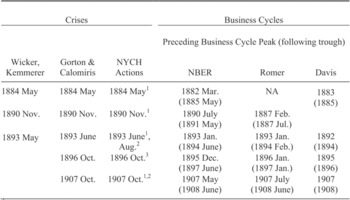
First column gives Wicker's (2000, p. 9) months of “panic onset,” which are the same as Kemmerer's (1910, p. 222) months “panic began” or “crisis began.” Second column is Calomiris and Gorton's “height of panic” (1991, table 4.1). NYCH actions from Wicker (2000), Calomiris and Gorton (1991, p. 114). Business cycle dates from NBER website, Romer (1994), and Davis (2006).
OUR DEFINITION OF FINANCIAL CRISES
Our definition of crises is conventional. Following O. M. W. Sprague (1910), Wilson, Sylla, and Jones (1990), Calomiris and Gorton (1991), Elmus Wicker (2000) and others, we define a national financial crisis as a general run on banks in New York City, and identify such events objectively by the actions of the New York Clearing House (NYCH). When NYCH directors perceived that a general run was underway or imminent, they authorized the issuance of clearinghouse loan certificates (Wicker 2000, p. 116). Certificates substituted for cash in interbank payments, freeing up banks’ cash to pay off withdrawals. They were issued when a bank applied to the NYCH for a loan and NYCH agents deemed the bank a good risk after examining its books (which may have helped verify the bank's solvency to the public).
We are particularly interested in the era when America was part of the international gold standard, from 1879 to 1913. We do not include 1914 in our analysis because the outbreak of World War I created financial disturbances of obviously foreign origin. Table 1 lists the crises that occurred within 1879–1913 according to various studies.
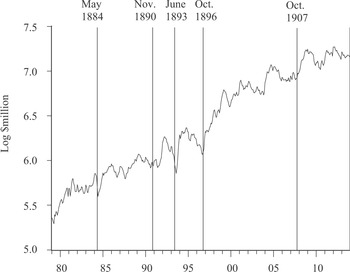
DEPOSITS IN NYCH MEMBER BANKS MONTHLY, JANUARY 1879–DECEMBER 1913 (with seasonal adjustment)

All studies identify crises in 1884, 1890, 1893, and 1907, when NYCH loan certificates were issued. Calomiris and Gorton (1991) identify an additional crisis in 1896, when the NYCH authorized certificates (because withdrawals had left many New York banks’ cash reserves below legal requirements) but no bank applied for a clearinghouse loan (New York Times 23 August 1896, 9; 25 August 1896, 4; 26 August 1896, 1, 10; 1 September 1896, 1).
Figure 1 plots the log of deposits in NYCH member banks at a monthly frequency with a seasonal adjustment.Footnote 1 There are obvious drops in deposits around the crisis dates of 1884, 1893, and 1896. In 1890, according to Wicker (2000), “The speedy authorization to issue loan certificates forestalled the spread of the disturbance” (p. 41); “An incipient panic had been nipped in the bud” (p. 47). In 1907 the first runs occurred at trust companies, which were not NYCH members. At the same point in time that the NYCH authorized loan certificates, it restricted cash payments which effectively froze deposits in NYCH banks. (The NYCH also restricted payments in 1893, but many weeks after it authorized certificates.)
A run on banks in New York City—rather than, say, Philadelphia or Chicago—meant a national crisis because of New York's central role in the financial system. New York banks were a key source of funding for the shadow banking system of the era—private banks, brokerage houses, and commercial paper houses. They arranged most loans to firms and individuals who borrowed short term to finance purchases of long-term securities, through overnight “call money” loans or 2–6 month “time money” loans (Myers 1931, pp. 265–87, 335). On the liability side, New York banks drew interbank deposits—”bankers’ balances”—from all parts of the country. Deposits in a New York “correspondent” bank (or in a regional money center bank that held deposits in New York) were an important liquid asset to nearly all out-of-town banks (James 1978).
An increase in banks’ demand for cash reserves or the nonbank public's demand for cash, anywhere in the country, was ultimately covered by withdrawals of bankers’ balances and shipments of cash out of New York (unless it was offset by a decrease in demand somewhere else). Thus, widespread bank runs in the hinterland were quickly transmitted to New York, while a run or restriction of payments in New York triggered payments restrictions by other cities’ banks and clearinghouses. As a run on New York hindered many types of financial intermediation, it raised the cost of credit and tightened credit rationing (Mishkin 1991). A New York run also raised transactions costs, because New York bankers’ balances were the chief medium of intercity payments: during a crisis payers had to resort to long-distance cash shipments (James, McAndrews, and Weiman forthcoming).
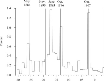
All but one of the crisis dates in Table 1 coincided with extraordinarily high rates of bank failures. Benjamin S. Bernanke (1983) uses a deposit-weighted failure rate (the fraction of deposits in banks that had been taken over by authorities) to measure the degree of financial disintermediation in the 1930s. For the pre-1914 era, the statistic closest to Bernanke's measure is an asset-weighted failure rate, available at an annual frequency for twelve-month spans ending with June.Footnote 2Figure 2 shows that this series spikes in the spans containing the crises of 1884, 1893, 1896, and 1907. On this measure, 1896 was indeed a crisis. We classify it as such for the regressions we report below, but our results do not depend on it. The 1890 episode was an exception: though generally considered a crisis, it was not coincident with a spike in bank failures.
BANK FAILURE RATE, 1879–1913, WEIGHTED BY ASSETS* ANNUAL, TWELVE-MONTH PERIODS ENDING JUNE

EXISTING LITERATURE ON CAUSES OF CRISES
Theoretical models and empirical studies have examined causes of runs on financial intermediaries in many times and places. Generally, they show that runs can occur when lenders to intermediaries, e.g., bank depositors, observe a decline in market values of intermediaries’ liquid assets, or come to believe intermediaries’ illiquid assets will not pay off: this means some intermediaries may be insolvent. Lenders may withdraw funds from most intermediaries even if they believe only some are insolvent, if they are unsure exactly which intermediaries are at risk (Gorton 2010), or if they expect the news to cause other lenders to withdraw (Morris and Shin 2000) in the type of liquidity crisis described by Douglas W. and Diamond and Phillip H. Dybvig (1983). A shock is more likely to set off a crisis if it occurs at a time when funds were already being withdrawn from intermediaries (Chari 1989). In the case of the pre-1914 United States, the potential cause of a financial crisis would be a set of events, exogenous to the American macroeconomy, that created conditions endangering the solvency of New York banks, especially if they occurred at a time when deposits were already being withdrawn from New York banks.
1890 and 1907: Contagion from Europe
In the post-World War II era, “sudden stops” of foreign investment triggered many financial crises in capital-importing countries of Latin America and Asia (Calvo and Reinhart 1996; Kaminsky, Reinhart, and Vegh 2003). According to many pre-1914 contemporaries and modern economists (e.g., Sprague 1910, p. 132; Fels 1959, p. 167; Friedman and Schwartz 1963, p. 104, 156; Eichengreen 1992, p. 51; Bordo 2006; Reinhart and Rogoff 2009, p. 243), the American crises of 1890 and 1907 were caused by sudden stops of foreign investment from Europe. This is plausible because an exogenous decline in foreign demand for American assets would tend to depress American stock prices and real activity. A drop in stock prices threatened New York banks as it could bring defaults on their loans to stock market “speculators.” A recession could bring defaults on business loans and threatened banks all over the country, draining their interbank deposits from New York.
Through most of the pre-1914 era, the United States imported capital from Europe. Europeans held large fractions of outstanding American securities (Wilkins 1989). At short maturities, Americans borrowed in London by selling “finance bills,” 1–3 month paper “drawn” on a London bank like a trade bill but collateralized by American stocks and bonds like New York time money (Margraff 1912, pp. 34–42). Through international arbitrage, a hike in European interest rates or a European sell-off of securities in general would tend to raise American interest rates and lower prices of American securities.
The 1890 episode was the most notorious European financial disturbance of the pre-1914 era, the “Baring Crisis.” Events in South America had caused European investors to fear defaults on Argentine bonds, depressing those bonds’ prices and endangering the solvency of London financial houses exposed to them, including Barings’. In July 1890 Barings’ and others began fire sales of good assets, including American securities, to raise liquid funds (Noyes 1898, p. 157; Lauck 1907, p. 64; The Economist (Supplement, Feb. 21, 1891); Wilkins 1989, pp. 194, 222, 471). Meanwhile, a monetary tightening by the Bank of England hiked rates on London bills, including American-issued finance bills (Sprague 1910, p. 133).
The year 1907 saw sharp hikes in European bill rates, due to tightening by the Bank of England and other European central banks in response to a persistent international gold drain. According to Kerry A. Odell and Marc D. Weidenmier (2004), the gold drain reflected payments by European insurance companies for damage from the San Francisco earthquake of 1906. The Bank took further actions to choke off American finance bill borrowing, specifically (Sprague 1910, p. 241; Noyes 1898, p. 358; Sayers 1976, pp. 54–56).
An increase in American interest rates due to foreign events, hence exogenous to American conditions, would tend to depress American real activity and could precipitate a business cycle downturn. Calomiris and Gorton (1991) argue that cyclical downturns were the proximate cause of all of the crises listed in Table 1: when people perceived a downturn was underway, they feared a wave of defaults on banks’ business loans; panics in the hinterland due to fears for local banks were transmitted to New York as out-of-town banks withdrew bankers’ balances to build up their own cash reserves. To support their argument, Calomiris and Gorton point out that all crises occurred in the midst of cyclical downturns according to the NBER business cycle chronology, and all crises were preceded by big drops in stock prices. They argue these stock price declines indicated the public expected a recession, which would hit corporate earnings.
Aside from its role as an indicator of expected recession, a drop in stock prices could be a more direct result of foreign financial disturbance. Stock prices reflect required returns to long-term securities as well as expected corporate earnings. An increase in required returns due to international factors would depress American stock prices for any given expectations of future earnings. A drop in stock prices was also a direct threat to the solvency of New York banks, especially. Some New York banks lent to brokerages and other stock “speculators” who could not repay if stock prices fell sharply. The problem was not ordinary callmoney or time money loans. These were collateralized with large “haircuts”—margins between collateral value and loan amount—to protect the lender against drops in collateral value.Footnote 3 We have found no evidence of runs due to fears of losses on such loans. The problem was rather that banks made large unsecured loans to speculators, sometimes illicitly, and depositors did not know exactly which banks had done so. Some of the most conspicuous New York runs in 1884, 1890, and 1907 occurred for this reason (Hanes and Rhode 2012).
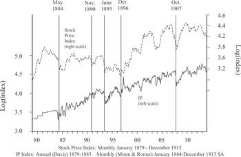
STOCK PRICES AND INDUSTRIAL PRODUCTION, 1879–1913

All the crises in Table 1 were, indeed, preceded by large declines in stock prices. All but one took place during cyclical downturns—the exception is, again, 1890. These patterns are apparent in Figure 3, which plots a monthly index of American stock prices and a seasonally adjusted version of Miron and Christina D. Romer's (1990) monthly industrial production (IP) index. The Miron-Romer index begins with January 1884. For earlier years, we link it to Joseph H. Davis’ (2004) annual IP index, which covers the entire nineteenth century.Footnote 4 Right-hand columns of Table 1 give dates of business cycle turning points around crises according to the old NBER chronology and two other chronologies based on more recent research. Romer's (1994) is based on the monthly IP index so it does not cover 1884. She shows that the NBER chronology, which was developed prior to the adoption of the modern definition of business cycles, places some peaks too early and includes some nonexistent downturns (when nominal variables fell but real variables continued to grow). Davis’ (2006) peaks and troughs are simply those apparent in his annual IP index. All the chronologies place a downturn prior to the crises of 1884, 1983, 1896, and 1907. Only the NBER's dates a downturn near 1890.
What About 1884, 1893 and 1896?
Like 1890 and 1907, the crises of 1884, 1893, and 1896 were preceded by cyclical downturns and stock-price declines. But none can be plausibly attributed to a foreign financial crises or central bank tightening.Footnote 5 A political factor that contributed to these crises, but did not trigger them, was the perceived danger that the United States would link the dollar to silver and float against gold. “Silver risk” contributed to crises by reducing international demand for American securities.Footnote 6 Silver risk appears to have become negligible after the 1896 presidential election, which was taken to signal firm commitment to the gold standard (Friedman and Schwartz 1982, pp. 513–17). The literature does not claim that exogenous hikes in silver risk set off crises but rather that potential silver risk was crystallized by, and amplified, cyclical downturns and financial crises already underway.Footnote 7 The more-or-less exogenous political events that created silver risk—the 1878 Bland-Allison Act, the 1890 Sherman Silver Purchase Act—occurred years before the crises in question.
Monetary Shocks from Agriculture
The quantity of a crop that is harvested varies greatly from year to year. Some harvest fluctuations may be endogenous responses to macroeconomic conditions, but agricultural output is also uniquely affected by obviously exogenous factors: weather and pests. Scholars have considered two possible channels from harvest fluctuations to pre-1914 American financial crises. The first runs through high-powered money demand. America's three great staple crops, cotton, corn, and wheat, were planted in or before the spring and harvested within a span of months from late summer through autumn—the harvest season.Footnote 8 Farmers were paid for their crops, and farmworkers received most of their wages, during or shortly after the harvest, creating a surge in demand for cash which fell off gradually to a low in early summer. The surge was accommodated by cash shipments from the northeast, funded largely by withdrawals of bankers’ balances from New York (Sprague 1903; Kemmerer 1910). V. V. Chari (1989) speculates that American financial crises occurred in years when agricultural conditions created especially large surges in cash demand and withdrawals of banks’ balances, leaving New York banks vulnerable to further shocks. To test this, Calomiris and Gorton (1991) look for a relation between harvest size and occurrence of crises, on the assumption that rural cash demand was positively related to crop production. They conclude “seasonal money demand shocks originating in the countryside cannot possibly be the cause of panics” (p. 148), as they find “years in which panics occurred in the fall… were not years of unusually large harvests for corn, wheat, and cotton” (p. 137).
A second possible channel runs through revenues from crop exports and the potential link between net exports and the money supply. Under the gold standard, for most countries the sum of net exports, international capital inflow and foreign investment income was balanced by an inflow of monetary gold from other countries. In the United States, the supply of high-powered money to banks and the public consisted of monetary gold plus currency (greenbacks, silver notes, national banknotes, silver coins) minus money held in U.S. Treasury vaults (Friedman and Schwartz 1963, pp. 124–34). Currency growth was unresponsive to economic conditions and mostly out of the Treasury's control.Footnote 9 On occasion, Treasury officials deliberately managed their reserves of vault cash to affect the money supply (Timberlake 1978) but these operations were limited by the degree of slack between expenditures, tax receipts, and bond operations. The Treasury did not generally sterilize international gold flows. Thus, the change in the American high-powered money supply was linked to export revenue, as an element in the balance of payments.
Cotton and wheat (raw wheat and wheat flour) were important American exports. For both crops, export revenue was positively related to the size of the harvest, and export-revenue fluctuations were large relative to the high-powered money supply (Davis, Hanes, and Rhode 2009). Thus, fluctuations in cotton or wheat harvests could produce substantial exogenous shocks to potential high-powered money supply growth. Contemporaries believed cotton and wheat harvests affected financial conditions through this channel (Sprague 1903, p. 50; Andrew 1906). Note it implies unusually large harvests of cotton or wheat would tend to reduce, not raise the probability of a financial crisis.
Milton Friedman and Anna Jacobson Schwartz (1963) argue that the crisis of 1893 was triggered by fluctuations in wheat harvests through this money-supply channel and the classic specie-flow mechanism. Wheat and wheat flour export revenue was extraordinarily high following the harvest of autumn 1891, partly because of a large harvest, an “accident of weather” (p. 107). The resulting gold inflow “fostered a spurt in the stock of money from 1891 to 1892” that interrupted a longer-term deflationary trend. A reversion to deflation in 1893 caused bank runs because “[l]oans that would have been good and banks that would have been solvent if prices had been stable or rising became bad loans and insolvent banks under the pressure of price deflation” (p. 108). Wheat export revenues remained low until “another one of those fortuitous combinations of good harvests at home and poor harvests abroad” in 1897, which contributed to recovery from the 1896 crisis (p. 140).Footnote 10
Davis, Christopher Hanes, and Paul W. Rhode (DHR) (2009) examine the relation between pre-1914 American business cycles and harvests of all three of America's staple crops, cotton, wheat, and corn, constructing instruments for harvest fluctuations from weather data. DHR find that, within 1879–1913, the size of the cotton harvest had positive effects on the following year's industrial production, gold inflows, and high-powered money supply growth, and negative effects on commercial paper interest rates. Wheat harvests had positive effects on gold inflow and money growth but no apparent effects on industrial production or interest rates. Corn harvests affected none of these variables. With respect to cotton, DHR find no systematic differences between OLS and IV coefficient estimates, and no evidence of reverse causality from business cycles to harvest fluctuations. Thus, it appears cotton harvest fluctuations in general, not just those due to weather, were exogenous to the macroeconomy.
DHR argue that a crop's macroeconomic effects reflected the relative intensity of its more immediate effects on export revenue and rural cash demand. To the degree that a bumper harvest boosted export revenue, it drew in gold, lowered interest rates, and stimulated real activity. To the degree that a harvest boosted cash demand, it drew in gold but raised interest rates and depressed real activity. Corn harvests had no apparent macroeconomic effects because they had little effect on export revenue or cash demand: little corn (or corn meal) was exported; relatively little was even sold off the farm for cash income. Wheat harvests had strong positive effects on export revenue and cash demand, so wheat affected gold flows but not, on net, interest rates and real activity. Cotton harvests had strong effects on export revenue, but, unlike wheat, relatively weak effects on cash demand. Thus, a big cotton harvest lowered interest rates and raised industrial production. Cotton's export-revenue effect was relatively strong partly because cotton exports were a large share of domestic production: export revenue was very large relative to farmers’ income from sales of the crop. For wheat, exports (in the form of wheat and wheat flour) were a smaller share of production, so export revenue was smaller relative to crop sales. It is also possible, DHR argue, that cotton's cash-demand effect was relatively weak because Southern agricultural institutions tended to substitute merchants’ and landlords’ credit for cash balances (pp. 1682–86, 1708–11).
DHR do not examine the relation between harvests and financial crises. In this article, we take on that task.
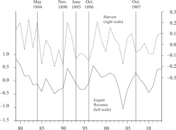
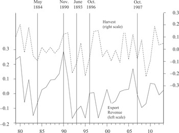
Figures 4 and 5 plot fluctuations in wheat and cotton harvests and export revenues. The top line in each figure is the deviation from a quadratic time trend (over 1869–1913 to match results we will present below) in the log of a year's autumn harvest, in bushels or bales. The lower line is the deviation from a similar quadratic time trend in “real” revenue from exports of each crop (cotton or wheat and wheat flour).Footnote 11
WHEAT HARVEST AND DEFLATED EXPORT* REVENUE, 1879–1913 LOGS, DEVIATIONS FROM TREND

From the figures, it is obvious that harvest fluctuations were just one factor affecting crop export revenue. Wheat revenue was high in 1907 despite a poor harvest. Cotton revenue was low in 1898 and 1908 despite big harvests. Some of the other factors affecting export revenue must have been endogenous to macroeconomic conditions: e.g., industrial demand for raw materials. Thus, we do not argue that export-revenue fluctuations in general were exogenous shocks to the macroeconomy. Our focus is on export-revenue fluctuations due to harvest fluctuations.
COTTON HARVESTS AND DEFLATED EXPORT REVENUE, DEVIATIONS FROM TREND, 1879–1913

Recall Friedman and Schwartz attribute the crisis of 1893 to a drop-off in wheat export revenue after 1891. That drop-off is apparent in Figure 4. It is clearly due, at least partly, to a decrease in the size of the American harvest. But Figure 5 shows something Friedman and Schwartz missed. The lower line of Figure 5 indicates that the cotton harvest prior to 1893, that is the harvest of autumn 1892, generated extremely low export revenue. The harvests prior to 1884 and 1896 also generated extremely low export revenue. The two crises that can be accounted for as the result of sudden stops, 1890 and 1907, were different: neither was preceded by a cotton harvest that generated low export revenue. The crisis of November 1890 was coincident with a cotton harvest that generated extremely high export revenue. The upper line of Figure 5 shows that the low cotton revenues of 1883, 1893, and 1896 were all associated with poor harvests. The high revenue of 1890 was associated with a bumper crop. Importantly, according to contemporaries the poor harvests of 1883, 1892, and 1895 and the good harvest of 1890 were all due to the exogenous factors of pests and weather.Footnote 12
To check whether the relation between financial crises and cotton harvest fluctuations apparent in Figure 5 holds for wheat as well, we ran a probit regression with the left-hand side variable equal to one in years with crises, and the previous years’ cotton and wheat harvest fluctuations (as in the figures) on the right-hand side, over 1879–1913 (harvests of 1878–1912). To account for the foreign financial shocks of 1890 and 1907, we removed those years from the sample.Footnote 13 The coefficient on cotton is negative and significantly different from zero at the 5 percent level; the wheat coefficient is much smaller and far from significance: 
HARVESTS AND FINANCIAL CONDITIONS: HYPOTHESES
We argue that the crises of 1884, 1893, and 1896 were in fact triggered by the poor cotton harvests of 1883, 1892, and 1895. Moreover, the bumper cotton harvest of 1890 may be largely responsible for the stability of real activity and the banking system in the wake of the Baring Crisis. The channel from cotton harvest fluctuations to financial conditions ran through the balance of the crop's effects on export revenue versus rural cash demand. Because cotton's export-revenue effect was relatively strong, a poor cotton harvest tended to create conditions that endangered the solvency of New York banks: a decline in stock prices and a cyclical downturn, at a time when deposits were already being withdrawn. Through the same channel, a bumper cotton harvest tended to counteract the effects of an exogenous sudden stop of foreign investment, that is a decrease in international demand for American assets due to interest rate hikes or financial disturbances in Europe.
In this section, we lay out our argument and its implications for observable variables. In the following section, we will present results of regressions that test those implications.
Money Supply Growth, the Balance of Payments, and the Current Account
In the gold standard United States, growth in the high-powered money supply from one period to the next was determined by the net inflow of monetary gold, the change in the supply of non-gold currency, and the change in the quantity of high-powered money sequestered in Treasury vaults. Thus, we describe the change in the log of the real money supply across a span of time as Δ(m – p) = g + z − Δ p where m is the high-powered money supply, p is the American price level, g is the inflow of monetary gold, and z represents the other money supply factors (expressed as a fraction of the previous period's money supply).
The balance of payments is the sum of the current account and the capital account. The current account—net exports less the net outflow of factor payments and transfers—might be affected by the level of real nonagricultural activity, denoted y, through American demand for imports. Net exports might also be affected by the relative price of foreign goods, as determined by the domestic price level p, the foreign price level p*, and exchange rates. Variations in the key exchange rate, against sterling, were large enough to affect short-term returns to foreign assets but too small to matter for trade.Footnote 14 Thus, we describe the current account (in real value, scaled by the average magnitude of its fluctuations relative to trend money growth) as a function CA(y−,(p –p*)−) + ɛCA. Superscripts in the function give the sign of a partial derivative: hence CAy < 0, CA(p – p*) < 0. The disturbance term ɛCA represents exogenous shocks to the current account, such as variations in export revenue due to exogenous fluctuations in an export crop's harvest.
The Capital Account and Imperfect Capital Mobility
The capital account reflects the change in net international demand for a country's assets. International demand for American assets must have been sensitive to returns on American versus European assets. Europeans traded American stocks and bonds in European markets as well as New York, with rapid arbitrage across the Atlantic. There was also arbitrage at the shorter maturity of bills. London was the central bill market of Europe.Footnote 15 Americans financing security portfolios shifted between London finance bills and New York time money depending on relative interest rates and expected exchange rates (Morgenstern 1959, p. 527). Some firms borrowed in London through finance bills to lend time money in New York (Margraff 1912, p. 41). Arbitrage between London bills and matching maturities in New York also operated through the mechanics of foreign exchange (Goodhart 1969). Except at times when perceived silver risk was high, expected future changes in the exchange rate were small relative to variations in interest rates. Thus, international arbitrage tended to equalize both bill maturity interest rates and expected returns to long-term securities between New York and European financial centers, especially London.
Within New York, commercial paper was a very close substitute for time money, from a lender's point of view. Unlike today, there was no active secondary commercial paper market, so commercial paper was about as illiquid as time money loans. Thus, changes in New York commercial paper rates were highly correlated with changes in time money rates.Footnote 16 Commercial paper was distributed throughout the United States by national dealers. Outside New York, it was the only available short-term open market investment. For a hinterland bank, commercial paper rates were the opportunity cost of short-term loans to local borrowers. Through commercial paper, therefore, short-term interest rates across the United States were linked to New York rates, and therefore European rates.
However, there is no reason to believe international arbitrage was sufficient to equalize expected returns in the United States and Europe, to the extreme of perfect capital mobility. European investors did not view American and European assets as perfect substitutes: in London, realized risk-adjusted rates of return were consistently higher for American securities even after the diminution of silver risk in 1896 (Edelstein 1982, pp. 157–58). Many empirical studies have rejected the hypothesis that uncovered interest rate parity (UIP) held between London bills and New York time money or commercial paper (Giovannini 1993, pp. 133–36; Foster 1994).Footnote 17 Demand for American assets was as depicted in models of “imperfect” international capital mobility (e.g., Kouri and Porter 1974). We describe the capital account as a function KA(Δ (i − i* − ɛEe)+) + ɛKA, where the benchmark foreign return i* would be best indicated by the open market bill rate in London. The corresponding American return i corresponds to interest rates for time-money or commercial paper, or to expected short-term returns to American stocks and bonds. ɛEe is the expected increase in the New York price of London sterling, which would be affected by perceived silver risk. ɛKA accounts for any other factors that might affect demand for American assets.
Demand for High-Powered Money
As the expected asset return relevant for capital flow i was linked to commercial paper rates, it would be related to demand for high-powered money. For the public and out-of-town banks, commercial paper rates represented the opportunity cost of holding cash. Aggregates of deposits and cash held by the public for the pre-1914 era show a normal money-demand relation to interest rates and national income or wealth (Friedman and Schwartz 1982). Thus, we describe demand for real high-powered money balances as L(y+, i−) + ɛmd. The disturbance term ɛmd represents exogenous shocks to high-powered money demand, such as variations in rural demand for cash due to exogenous fluctuations in a crop's harvest.
Interest Rates, Output, and the Price Level
Relations between interest rates, the price level, and real activity were governed by a constraint on long-run trend inflation imposed by the gold standard. For all gold standard countries, trend inflation was largely determined by the balance between world gold production, growth in real output and financial innovations in the use of monetary gold. There was little, if any, serial correlation in inflation from year to year. Judging from the behavior of interest rates, expected inflation at both long and short horizons was always close to zero and remarkably unresponsive to economic events (Barsky 1987; Barsky and Delong 1991; Bordo and Dewald 2001).
Under stable trend inflation, an expectations-augmented Phillips curve of either the Old-Keynesian or New Keynesian variety implies a positive relation between inflation and output along the lines of the original Phillips curve, rather than the “accelerationist” Phillips curve of the postwar era (Alogoskoufis and Smith 1991; Hanes and James 2012). Thus, we describe the change in the price level Δp as a function of nonagricultural real activity π(y+)+ ɛp. (The last term accounts for any extraordinary changes in inflation expectations, as well as “supply shocks.”)
Also, a positive shock to nominal interest rates would raise real interest rates and reduce real spending. Empirical studies of postwar data generally find that an exogenous shock to interest rates affects real spending and output after about six months, with the strongest effect appearing after about a year (e.g., Christiano, Eichenbaum, and Evans 2005). We are aware of no evidence that the lag was shorter in pre-1914 America. Thus, we describe y in a period as determined by a function of the interest rate in the prior period E(i−1+, (p − p*)−)+ ɛIS. In this context, a period must be about six months. We allow for an effect of the relative American price level on the volume of spending directed to domestic output (and foreign demand for exports). The last term accounts for exceptions to the usual pattern for expected inflation (which would affect the relation between nominal and real interest rates). It also accounts for extraordinary disturbances to the operation of financial intermediaries which would affect the supply of credit to potential borrowers (as in Woodford 2010).
Effects of Harvest Fluctuations
An exogenous fluctuation in the harvest of cotton or wheat meant a shock to export revenue reflected in ɛCA, and a shock to high-powered money demand reflected in ɛmd. The timing of the shocks was important. Foreign payments for cotton and wheat exports began within the autumn harvest season and continued through the early months of the following year (Kemmerer 1910, pp. 136–40). Taking a period to be about six months and letting h denote exogenous fluctuations in a crop's harvest, we describe the export-revenue effect of a harvest fluctuation as a disturbance ∂ɛCA/∂h > 0 that occurs within one period—period 1. Another period—period 2—passes before the next harvest season. The harvest's money-demand disturbance ∂ɛmd/∂h occurs within period 1 and persists through period 2.Footnote 18 Let (x1 − x0) denote the change in a variable to the harvest period 1 from period 0 prior to the harvest. Within the harvest period, the size of the harvest cannot affect real activity y but it may affect the required asset return i1 depending on the value of ∂ɛCA/∂h relative to ∂ɛmd/∂h
![\[
\begin{array}
minus i1 minus i0)/minus_h = minus beta_1 [minus_e_{CA}/minus_h minus minus_e_{md}/minus_h]
where beta_{1} = 1 / (CA{p minus p*} minus Li
\end{array}
\](https://static.cambridge.org/binary/version/id/urn:cambridge.org:id:binary:36587:20160629041142101-0619:S0022050713000077_eqn1.gif?pub-status=live)
If ∂ɛCA/∂h > ∂ɛmd/∂h, the size of the crop's harvest has an immediate negative effect on i. If ∂ɛCA/∂h = ∂ɛmd/∂h, the crop's harvest does not affect i, even though it affects export revenue. In the post-harvest period 2, real activity y2 responds to the crop's effect on i in the harvest period, while i2 reflects the response of y2 as well as the initial disturbances to export revenue and money demand
![\[
\begin{array}
y_2 minus y_0 /h = beta_2 beta_1[eCA/h e_md/h] = minus beta_2 minus(i_1 minus i_0)/h
where beta_2 equal E_i /(1 E(p minus p*)p_y)
\end{array}
\](https://static.cambridge.org/binary/version/id/urn:cambridge.org:id:binary:58813:20160629041142101-0619:S0022050713000077_eqn2.gif?pub-status=live)
![\[
\begin{array}
part(i_2 minus i_0) / part h equal (1 minus beta_1 beta_2 beta_3) beta_1 [.eCA/.h .emd/.h] = (1 . beta_1 beta_2 beta_3)) .(i1 . i0)/.h
where beta_3 = (1 . CA(p-p*)) py . CAy + Ly
\end{array}
\](https://static.cambridge.org/binary/version/id/urn:cambridge.org:id:binary-alt:20160715183130-01751-mediumThumb-S0022050713000077_eqn3.jpg?pub-status=live)
Note that the harvest's effect on i may diminish from period 1 to period 2: that is because an increase in output tends to reduce net exports and boost high-powered money demand. Whether or not an export crop's harvest affects i and y, the size of the harvest will have a positive effect on gold inflow
![\[
\begin{array}
\partial {\rm{ }}g_1 /\partial h{\rm{ = }}\partial \left({m_1 - m_0 } \right)/\partial h = - {\rm{ }}L_i {\ss}_1 \left[{\partial \varepsilon ^{CA} /\partial h{\rm{ }} - \partial \varepsilon ^{md} /\partial h} \right]{\rm{ + }}\partial \varepsilon ^{md} /\partial h
\end{array}
\](https://static.cambridge.org/binary/version/id/urn:cambridge.org:id:binary:15386:20160629041142101-0619:S0022050713000077_eqn4.gif?pub-status=live)

where (g1 + g2) is cumulative gold inflow since the pre-harvest period.
Our hypothesis is that, for wheat, (∂ɛCA/∂h − ∂ɛmd/∂h) was about equal to zero. Thus, the wheat harvest affected gold flows, but not financial markets or real activity. For cotton, (∂ɛCA/∂h − ∂ɛmd/∂h) was positive. Thus, the cotton harvest affected required returns to American assets, which is to say interest rates for commercial paper or time money, within the harvest period, and real nonagricultural activity in the post-harvest period.
As cotton harvests affected commercial paper rates within the harvest period, they could have affected the volume of deposits in New York City banks at the same time. Out-of-town banks held bankers’ balances partly to satisfy regulatory reserve requirements, but bankers’ balances were usually far in excess of requirements and varied substantially from quarter to quarter (Myers 1931, pp. 237–39; Goodhart 1969, pp. 76–77). For a bank outside New York, the commercial paper rate was the opportunity cost of holding New York bankers’ balances. New York banks paid interest on bankers’ balances, but they held the rate nearly fixed across the pre-1914 era (James 1978, pp. 176, 265–67). Thus, increases (decreases) in commercial paper rates due to cotton harvest fluctuations should have been associated with decreases (increases) in New York deposits.
As i represents required returns to securities as well as interest rates, our hypothesis implies that cotton harvests must have affected prices of American stocks and bonds, within the harvest period. For any given expectations of future real activity and corporate earnings, an increase (decrease) in required returns would depress (boost) securities’ prices. Additionally, financial market participants might forecast the upcoming effect of the cotton harvest on real activity. That would reinforce the effect of a change in required returns: on stock prices, by changing expectations of future corporate earnings; on bond prices, by changing probabilities of future defaults. In any case, in the post-harvest period the realized change in real activity would affect stock prices.
Through these channels, a poor cotton harvest could create all the conditions for a financial crisis by the post-harvest period. Thus, a poor cotton harvest could trigger a financial crisis. The occurrence of a financial crisis could be associated with many more disturbances, such as a decrease in ɛIS or an increase in ɛEe (due to heightened silver risk). Many of these disturbances which would tend to reinforce the effects directly due to the harvest's export-revenue shock. But the effects described by equations 1–5 are independent of the occurrence of a financial crisis.
With respect to observable variables, our hypothesis implies that the size of the cotton harvest should have negative effects on commercial paper rates, and positive effects on New York deposits, stock, and bond prices, within the harvest season. The cotton harvest's effect on industrial production should appear with a lag, about six months after the appearance of effects on financial variables. All of these effects should appear prior to the occurrence of a financial crisis and whether or not a crisis follows. The wheat harvest should affect international gold inflow, but not financial variables. The corn harvest should not affect financial variables or gold inflow.
Call Money Rates
Our hypothesis does not have clear implications for call money rates. Call money was not subject to direct international arbitrage. There are many contemporary references to American borrowing from London at the maturity of time money, but we have found no references to trans-Atlantic lending at the overnight maturity.
A link between call money rates and i would come through time money or commercial paper. Generally, one would expect rates for these bill maturity assets to equal the expected return to call money lending over the appropriate horizon plus a liquidity premium. Descriptions of the call money market by contemporaries (e.g., Woodlock 1908; White 1910) and later observers (Myers 1930, pp. 265–87; Goodhart 1969) suggest the premium varied greatly and depended on a distinct supply and demand for call money funds. Borrowers attempted to finance a fairly stable fraction of their portfolios’ value with call money. They were reluctant to substitute call-money for time money even when call money rates were especially low, for fear they would be unable to roll over the loans (Woodlock 1908, p. 29). Thus, an increase in American securities’ prices raised the demand for call money loans as it raised the value of borrowers’ portfolios and collateral. On the supply side, the bulk of call money lending was by New York banks, which usually tried to match their holdings of this low return but uniquely liquid asset to the volume of bankers’ balances, a volatile liability. The supply of call money increased with the volume of bankers’ balances. According to Margaret G. Myers (1930, p. 275):
Call money rates may be high under two conditions: when a rapid drain of funds to the interior has reduced the surplus funds of New York banks and caused a reduction in the amount of their loans on call; or when a rising movement of security prices increases the demand for call loans…Call rates might be low under the two opposite conditions; when there is a large volume of surplus funds in the market under circumstances which make it inadvisable to invest them otherwise than at call, or when the security market is so sluggish that it does not require even the small amount of funds available.
A study of call money liquidity premiums with proper accounting for the details of interest rate definitions, timing and causality is beyond the scope of this article. But the relation between call money rates, securities’ prices, and New York deposits posited by Myers is obvious in our data (Hanes and Rhode 2012). Thus, a poor cotton harvest could tend to lower call money rates by reducing time money rates, but it could also tend to raise call money rates by depressing securities’ prices and draining bankers’ balances.
Interaction Between Cotton Harvests and Foreign Financial Conditions
An increase in foreign interest rates due to tightening by foreign central banks corresponds to an increase in i*. A decrease in foreign demand for American assets due to fire sales by European investors in an event such as the Baring Crisis corresponds to a decrease in ɛKA. How would these shocks interact with the cotton harvest's effects on export revenue and money demand? Within the harvest period, the net effect on i would be

with the corresponding effect on real activity in the following period. Thus, as a big cotton harvest means a large value of (∂ɛCA − ∂ɛmd), it would tend to counteract the financial and macroeconomic effects of interest rate hikes or other financial disturbances in Europe.
What If America Had a Central Bank?
If America had a central bank, its open market operations and discounting would affect z as they affected the supply of non-gold high-powered money—not only currency, but also financial institutions’ balances at the central bank. Thus, a central bank could adjust z in response to cotton harvests. Within the harvest period, the net effect on i would be
![\[
\begin{array}
\partial i = - {\rm{ }}{\ss}_1 \left[{\partial \varepsilon ^{CA} - {\rm{ }}\partial \varepsilon ^{md} {\rm{ + }}\partial z} \right]
\end{array}
\](https://static.cambridge.org/binary/version/id/urn:cambridge.org:id:binary:38825:20160629041142101-0619:S0022050713000077_eqn7.gif?pub-status=live)
An American central bank could have counteracted the financial effects of cotton harvest fluctuations by ensuring that ∂z/∂h = − ∂ɛCA/∂h + ∂ɛmd/∂h. A central bank could achieve this by buying (selling) domestic securities in response to a poor (abundant) harvest, or simply by setting its discount rate slightly above the normal market rate for the season. Cotton harvests would then, like wheat harvests, affect international gold flow but not financial markets or real activity.
HARVESTS AND FINANCIAL CONDITIONS: ECONOMETRIC ANALYSIS
We examine harvests’ actual effects on financial markets by regressing changes in observable variables on deviations from trend in the size of the cotton, wheat, and corn harvests. Estimated coefficients show how effects played out over time across the harvest season and through the following calendar year. To ensure that the apparent effects of cotton harvests held whether or not a crisis occurred in the following year, we run regressions on samples that exclude harvests preceding the calendar year containing a crisis (autumn 1883, 1889, and so on). As our hypotheses mainly have to do with the operation of financial markets outside crises, we also repeat all regressions on samples excluding harvests that took place within the calendar year containing a crisis (autumn 1884, 1890, and so on). Results from this last set of samples are similar to those from the full sample. They are presented in Hanes and Rhode (2012).
We present results from 2SLS using regional weather data as instruments, as well as from OLS. In 2SLS first-stage specifications follow DHR (2009), who give details on the weather data and the instruments’ strength. Each crop's harvest is projected on a different set of weather time-series (different geographic regions, different months’ precipitation and temperature). Prior information—early twentieth-century statistical studies of weather effects on crop yields—guided the choice of weather variables for each crop. Recall DHR's results indicate that cotton harvest fluctuations in general, not just those due to weather, were exogenous to macroeconomic conditions. Thus, we do not expect 2SLS to show different patterns from OLS here. We present the 2SLS results for robustness.
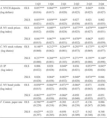
Results show the patterns we hypothesized. The deviation from trend in the cotton harvest had positive effects on American stock prices and NYCH bank deposits within the harvest season, and positive effects on IP about six months later. The cotton harvest had negative effects on American bond yields (which move inversely to bond prices) and commercial paper rates, with the same timing as the stock price effects. That indicates stock prices were reflecting a general effect of the cotton harvest on required returns to American assets subject to international arbitrage. British stock prices and British bond yields do not show these effects. American call money rates respond weakly, if at all, to the cotton harvest. Cotton's effects on American financial markets and IP appeared prior to the onset of financial crises and whether or not a crisis occurred. Deviations from trend in wheat and corn harvests do not have any of these effects on financial and macroeconomic variables.
Our hypotheses do not have clear implications about exactly when in the year cotton harvest fluctuations should have begun to affect financial variables. In principle, cotton harvest fluctuations could be correlated with changes in asset prices prior to the harvest season. Sophisticated investors could have traded on forecasts of the coming harvest, which were available beginning in June. On the other hand, it is clear that contemporaries viewed harvest forecasts as unreliable until the onset of the harvest season in August.Footnote 19 Certainly, contemporaries had neither the techniques nor all of the weather data we use ourselves to forecast harvests as IV's. We look for “effects” of harvest fluctuations on financial variables prior to the third quarter of the harvest year, but find no significant relations.
Statistical Specifications
Crop production trends were defined to be quadratic in time over 1869–1913 to match DHR (2009). (HP trends or quadratic trends over 1878–1913 gave similar results.) We want to pin down the seasonal timing of harvests’ effects but the timing of harvests themselves varied from year to year. The cotton harvest, for example, could peak in September one year, October the next. To allow for some slack, we average monthly series up to a quarterly frequency.
Our main dependent variables are changes in stock prices, bank deposits, and so on from a pre-harvest value to Q3 or Q4 of the harvest year, and to each of the four quarters of the calendar year following the harvest. The pre-harvest value is a four-quarter average up through Q2 of the harvest year, for variables known to be subject to strong seasonal influences in the pre-1914 era (industrial production, commercial paper, NYCH bank deposits, call money, London bills, New York stock volume [on stock volume seasonals see Owens and Hardy 1925]). For other variables, the pre-harvest value is the average for harvest-year Q2. Immediate effects of a harvest, within the harvest season, should appear in regressions with changes to harvest-year Q3 or Q4 of the harvest year on the left-hand side. Delayed effects appear in results for quarters of the following year. To look for “effects” of harvests on financial variables prior to the harvest season, we run regressions where the dependent variables are changes to Q2 of the harvest year from harvest-year Q1 or a four-quarter average up through harvest-year Q1.
Our samples begin with the harvest of autumn 1879, the first after the United States resumed gold payments, and stop at the end of 1913. For most variables all-harvest samples have 35 observations for harvest-year Q3 and Q4, 34 observations for following-year Q1-Q4. In the tables, coefficients and standard errors are scaled to the standard deviation of a cotton harvest fluctuation (0.12 for harvests 1878–1912); standard deviations for wheat (0.13) and corn (0.14) were similar. Thus, the tables give estimated coefficients and SE's multiplied by 0.12. On a causal interpretation, they give the effect of a one-standard-deviation harvest fluctuation.
Results
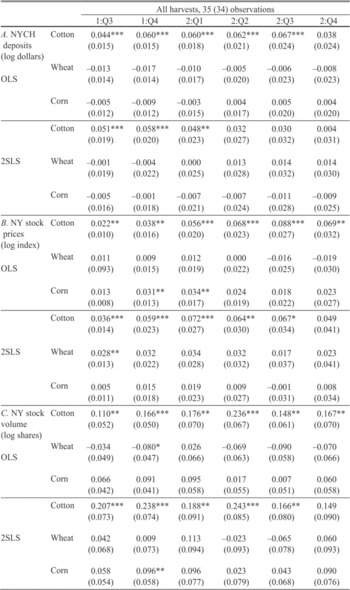
Tables 2, 3, 5, 6, and 7 show results from the sample including all harvests. For OLS, all three crops’ harvest fluctuations were included together. For 2SLS, we ran separate regressions for each crop. The harvest year is year 1; the following year is year 2.
For panels A and B in Table 2, dependent variables are changes in logs of NYCH bank deposits and the stock price index. For panel C, dependent variables are changes in NYSE trading volume (number of shares), another indicator of stock prices: in modern data, trading volume has a strong positive correlation with changes in stock prices (Karpoff 1987). For all of these financial variables, cotton coefficients are generally positive, and significantly different from zero at conventional levels, starting in harvest-year Q3 or Q4. Financial crisesoccurred in Q2 or later. Thus, cotton's effects appeared prior to the occurrence of any financial crisis. Wheat and corn coefficients do not show these patterns. For stock prices, they are positive and significant only in some cases. For deposits, wheat and corn coefficients are actually negative in many cases.
EFFECTS OF HARVEST FLUCTUATIONS ON NEW YORK DEPOSITS AND STOCK MARKET

*** Significant at the 1 percent level;** Significant at the 5 percent level;* Significant at the 10 percent level.
Notes:
Coefficient scaled to one SD log harvest fluctuation = 0.12, Standard errors, which are reported in parentheses, also rescaled.
Sources:
See the Data Appendix.

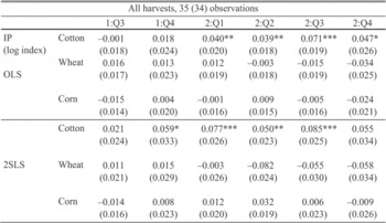
Table 3 shows results for industrial production. Samples are smaller here because the monthly IP index begins with January 1884. To define a pre-harvest value for the 1884 harvest season, we extrapolated from the change in Davis’ (2004) annual IP index as for Figure 3. (Coefficients from IP regressions were not substantially different if we began samples with the 1885 harvest.) For Q3 and Q4 of the harvest-year, cotton coefficients are not significantly different from zero; some are negative in sign. Cotton coefficients are positive and significantly different from zero for Q1 or Q2 of the following year, and are largest for following-year Q3. (None of the wheat or corn coefficients is positive and significantly different from zero.) Thus, cotton's effect on industrial production did not appear before the end of the harvest year, and was strongest about a year after the harvest.

Table 4 gives results from samples excluding harvests preceding calendar years containing crises. Coefficients in panels A through D show the same patterns as in Table 2. Thus, cotton harvests affected New York deposits, stock prices, and real activity whether or not they were followed by a crisis.
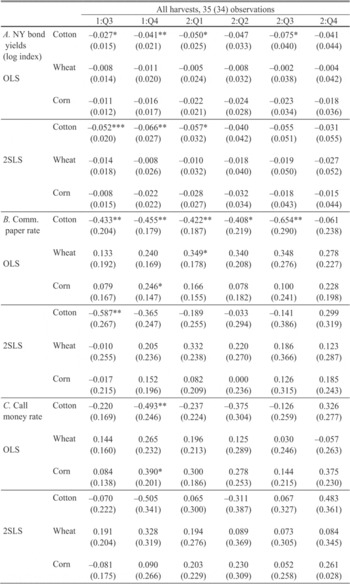
We hypothesized that cotton harvests could affect stock prices prior to industrial production through an effect on required returns on assets subject to international arbitrage. Cotton's positive effects on stock prices should thus be matched by negative effects on bond yields. The best indicator of American bond yields for the pre-1914 era is Frederick R. Macaulay's (1938) index of American railroad bonds’ yields to maturity. Panel A of Table 5 shows results with changes in this bond yield index as dependent variables. Cotton coefficients are indeed negative and statistically significant by harvest-season Q4.
Cotton harvests should also affect interest rates at the maturity of time money or commercial paper. There is no continuous series on time money rates for 1879–1913, but we can examine commercial paper rates. These results are in panel B of Table 5. Cotton coefficients are indeed negative and significantly different from zero in harvest-year Q3 and/or Q4. That is consistent with our argument that wheat harvests had relatively strong effects on money demand, and matches negative coefficients on wheat for NYCH deposits in Table 2, panel A. The previous section's argument also implied that cotton's interest rate effect could diminish in the post-harvest period, absent further shocks. In Table 4's results from the sample excluding pre-crisis harvests, cotton coefficients are positive and significant in the harvest season, small and not significantly different from zero in the following year.
The magnitude of cotton coefficients for commercial paper, in quarters where they are significantly different from zero, is about ten times the corresponding coefficients for bond yields in Table 5, panel A. That makes sense. As the maturity of the bonds in the yield index is at least ten years, the change in their yields could be about one-tenth of the change in short-term rates if market participants expected the latter to persist about a year, even if there were no changes in total premiums for bonds’ term, relative liquidity, and default risk.
The coefficient values in Tables 2 and 5 imply that stock prices fell about 1.75 percent for each 25 basis point increase in the commercial paper rate. We know of no evidence that would allow us to judge whether this is reasonable for the pre-1914 era, but it is roughly in line with patterns in modern American data. Roberto Rigobon and Brian Sack (2004) estimate that “an unanticipated 25-basis point increase” in the Fed's interest rate target, which is directly reflected in bill maturity rates, “results in a 1.7 percent decline in the S&P index” (p. 1567). Bernanke and Kenneth N. Kuttner (2005) find that an “unanticipated 25-basis point cut in the federal funds rate target” in a period when changes in the target affected bill rates about one-to-one, and could be expected to persist for about a year (their Figure 6), was “associated with about a 1 percent increase in broad stock indexes” (p. 1221).

Results for call money rates are in Table 5, panel C. Recall our essential argument—cotton harvests affected financial conditions through international asset markets—has ambiguous implications here: call money rates were not directly subject to international arbitrage, and there is reason to believe they would be positively affected by increases in securities prices. In fact, one of the cotton coefficients in this panel is negative and significant, but most are not.
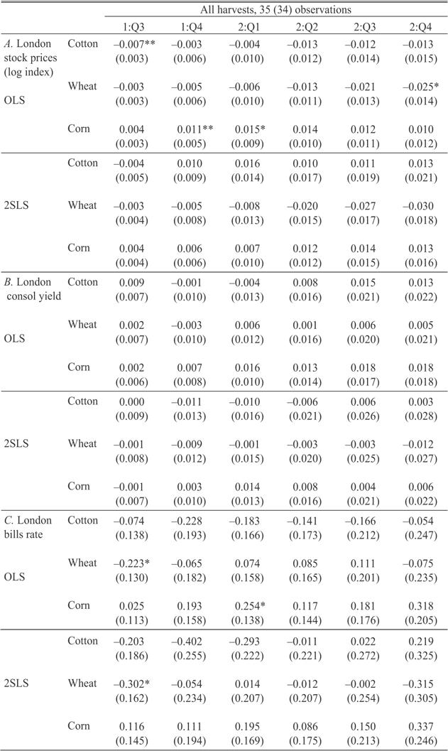
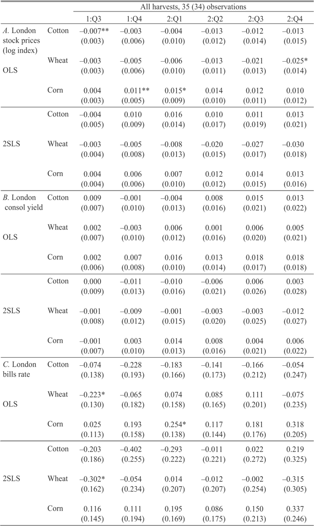
Results for British stock (equity) prices, consol yields, and bill rates are in Table 6, panels A-C. Our argument implies that cotton harvests should not affect these variables in the same way they affect American stock prices and interest rates. For bill rates and consol yields, no coefficient is significantly different from zero at the 5 percent level. For the stock price index, in OLS on the full sample the coefficient on cotton in harvest-season Q3 is significantly different from zero at the 5 percent level, but its sign is negative.
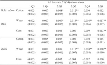
Key to our argument is that wheat harvest fluctuations did affect international gold flow and high-powered money supply, as shown by DHR (2009) in annual data, even though wheat harvests did not affect financial variables as cotton did. Table 7 shows results of regressions where the dependent variable is cumulative net gold inflow through the end of the quarter, as a fraction of the pre-harvest high-powered money supply. Coefficients on wheat as well as cotton are positive and many are significantly different from zero at 5 percent or better.
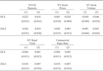
Finally, Table 8 shows results for changes to Q2 of the harvest-year, in the variables that show effects of cotton harvests within the harvest season: NYCH bank deposits, New York stock prices and trading volume, New York bond yields and commercial paper rates. None of the coefficients is significantly different from zero.
COTTON HARVESTS AND KEY VARIABLES IN CRISIS YEARS
Our regression results imply poor cotton harvests generally tended to lower stock prices, drain deposits from New York banks, and depress real activity. Earlier, we showed that the crises of 1884, 1893, and 1896 were all preceded by extremely poor cotton harvests, stock price declines, and downturns of real activity from cyclical peaks; 1893 and 1896 were also preceded by persistent declines in NYCH deposits. Returning to Table 1, note that the more reliable business cycle chronologies place the peaks preceding 1884, 1893, and 1896 around the beginning of the crisis year. The NBER date for the pre-1884 peak is much earlier, but recall Romer (1994) finds that many NBER peaks are dated too early. Annual industrial production peaked in 1883, so real activity must actually have peaked in late 1883 or 1884. This timing is consistent with the effect of a poor cotton harvest in the prior autumn: as the regressions with industrial production on the left-hand side give positive and significant coefficients for following-year Q1, they indicate that cotton harvests started to affect real activity around the beginning of the following year.

EFFECTS OF COTTON HARVEST FLUCTUATIONS PRIOR TO HARVEST SEASON

Notes:
Standard errors are in parentheses.
Source:
See the Data Appendix.
COTTON HARVESTS AND STOCK PRICES, HARVEST YEARS 1879–1912

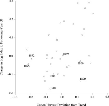
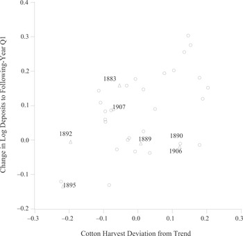
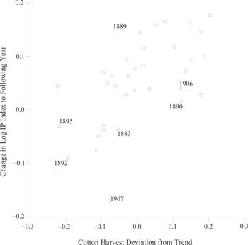
As further evidence that poor cotton harvests triggered these crises, we present scatterplots of cotton harvest deviations from trend (the same variable used in the regressions) against changes in stock prices, NYCH deposits, and industrial production. For stock prices in Figure 6 and NYCH deposits in Figure 7, the vertical axis is the change from the pre-harvest period to Q1 of the calendar year following the harvest. (Recall that all crises occurred in Q2 or later.) For industrial production in Figure 7, the vertical axis is the change in the log of Davis’ annual index from the harvest year to the following calendar year, so that we can include 1880–1883. Triangles mark the harvests that preceded crisis years.
COTTON HARVESTS AND DEPOSITS IN NYCH MEMBER BANKS, HARVEST YEARS 1879–1912

The scatterplots show that our regression results are not relics of a few extreme observations. More importantly, they show that the declines in industrial production and stock prices in 1884, 1893, and 1896, and the deposit declines in early 1893 and 1896, can indeed be explained by the prior years’ cotton harvests. The observations for the 1883, 1892, and 1895 harvests are not outliers. They are in line with the rest of the scatter, including or excluding the crisis-year observations.
Finally, recall we argued the crises of November 1890 and October 1907 were due to foreign financial disturbances, not poor cotton harvests. Our regression results imply that a large cotton harvest would tend to counter the effects of a foreign financial disturbance, as it boosted stock prices, deposits in New York banks and real activity. The cotton harvest of autumn 1890, coincident with the American echo of the London Baring's Crisis, was extraordinarily large and generated large export revenues. This can explain why the 1890 crisis, unlike the others, was not associated with an apparent decline in real activity or spike in bank failures.
The observations corresponding to the harvests of 1890 and 1907 are labeled in Figures 6–8. Consistent with our argument, in Figure 6 both of these harvests are obvious outliers: that is, the decline in stock prices across these harvest seasons cannot be accounted for by the cotton harvest. In Figure 8, also, the 1907 harvest is an outlier: the slightly below-trend harvest cannot account for the great decrease in industrial production from 1907 to 1908. The 1890 harvest observation is low relative to the scatter: most cotton harvests as large as 1890s were followed by large increases in industrial production. We cannot be precise about the possible interaction between the financial effects of the bumper cotton harvest versus the London financial crisis. Quantifying the possible effects of the latter is far beyond the scope of this article. But based on the figure, it is plausible that industrial production would have suffered an absolute decline in 1891, if not for the large cotton harvest of autumn 1890.
CONCLUSION
Five national financial crises, as conventionally defined, took place during the 1879–1913 gold standard era: in 1884, 1890, 1893, 1896, and 1907. All except 1890 were associated with cyclical downturns and waves of bank failures. Two, in 1890 and 1907, have already been accounted for as the results of sudden stops of European investment in the United States. We have presented evidence that cotton harvest fluctuations were the exogenous triggers of the other three, in 1884, 1893, and 1896, and may account for the anomalous stability of the American economy around 1890.
Cotton harvests affected New York bank deposits, stock prices and real activity in such a way that a good cotton harvest tended to counteract a foreign financial disturbance, and a poor cotton harvest tended to create crisis conditions in the next year. The channel to financial conditions ran through the effect of export-revenue shocks on required returns to American assets in international capital markets under the gold standard. The cotton crop and cotton export revenues were extremely large coincident with the crisis of November 1890 and extremely poor in the harvest seasons preceding 1884, 1893, and 1896. But cotton harvests affected financial conditions and real activity whether or not a crisis followed.
COTTON HARVESTS AND ANNUAL IP, HARVEST YEARS 1879–1912

For American monetary history, we have shown that contemporaries were right to argue that many crises could have been counteracted by an American central bank managing an “elastic” currency. The absence of financial effects from wheat harvests proves the point. Wheat harvest fluctuations affected international gold flows but did not disturb American financial markets because wheat harvest fluctuations had countervailing effects on high-powered money demand. For research on financial crises, we have shown that the factors triggering pre-1914 American crises had many repercussions, including cyclical downturns, which may be hard to distinguish from effects of crises.
Thanks to Michael Bordo, Charles Calomiris, Joseph Ferrie, John James, Jon Moen, Hugh Rockoff, Alan Taylor, Ellis Tallman, Marc Weidenmier, David Weiman, Eugene White, and Gavin Wright.
Appendix: Data Sources
“NBER” refers to the National Bureau of Economic Research Macrohistory database (data.nber.org/databases/macrohistory/contents/).
Bank Failures: Failed banks’ assets from U.S. Comptroller of the Currency (1921, table 39; 1932, pp. 5, 8.) The annual series given in Comptroller's reports for national banks is for periods ending with October, which does not match the series for other banks. But the detailed records in the reports also give details on closing of each national bank, including the exact date that a receiver was appointed. From these data, we calculated assets of failed national banks for the twelve months ending June to match the other banks.
International Gold Inflow to the United States: Monthly net gold export NBER 14112 (sign reversed).
Commercial Paper Rate: NBER 13002.
Railroad Bond Yield Index: NBER 13019A.
Stock Price Index: NBER 11025.
Number of Shares Traded on New York Stock Exchange: NBER 11002.
Call Money Rate: Larry Neal and Weidenmier (2003) collected each Thursday's call money rate from the New York Commercial and Financial Chronicle, beginning with November 27, 1880. When the rate was given as a range (which was most weeks), this is the low end of the range. Weidenmier kindly provided these data (at the time of this writing, available on his website ebutts05.tripod.com/nealweidenmiergsd). For January 1866 through December 1880, the Review of Economics and Statistics (July 1902, Vol. 2 Supplement 2, pp. 40–41) gives the monthly average of the weekly low rates of the Financial Review published by the Commercial and Financial Chronicle. We constructed our quarterly call money rate from a monthly series. Up through November 1880, this is the REStat series. Starting December 1880, it is the monthly average of the Neal and Weidenmier series.
London Equity Price Index: NBER 11012.
London Consol Yield: NBER series 13041 (2) linked to 13041 (3) at April 1884.
London Bill Rate: NBER 13016.
New York City Clearinghouse Member Bank Deposits, monthly averages: January 1879–December 1913 from Persons (1919, pp. 176–77, 180–81). Monthly data for 1878 calculated from weekly data in Andrew (1910).
Cotton, Wheat, and Corn Production: Susan Carter et al. (2006, Da696, Da718, Da756).
Cotton and Wheat Export Revenues: United States Department of Agriculture, Bureau of Statistics, Exports of Farm Products from the United States, 1851–1908, Bulletin 75 (USGPO, 1910) and Yearbook (1913, 1916).
Wholesale Price Index: Pearson, Warren, and Stoker (1932).