1 Introduction
Combustion assisted by swirl is a fundamental scientific problem where the interaction of fluid dynamics and reaction heat release forms complicated flow states, see, for example, Gupta, Lilley & Syred (Reference Gupta, Lilley and Syred1984), Sivasegaram & Whitelaw (Reference Sivasegaram and Whitelaw1991), Gutmark et al. (Reference Gutmark, Parr, Hanson-Parr and Schadow1992), Gupta, Lewis & Qi (Reference Gupta, Lewis and Qi1998), Paschereit, Gutmark & Weisenstein (Reference Paschereit, Gutmark and Weisenstein1998, Reference Paschereit, Gutmark and Weisenstein2000), Lieuwen & Yang (Reference Lieuwen and Yang2005), Syred (Reference Syred2006), Umeh, Rusak & Gutmark (Reference Umeh, Rusak and Gutmark2012), Durox et al. (Reference Durox, Moeck, Bourgouin, Morenton, Viallon, Schuller and Candel2013) and Candel et al. (Reference Candel, Durox, Schuller, Bourgouin and Moeck2014). These states include a reaction zone and a central recirculation (breakdown) zone (CRZ) around the domain centreline, at high flow swirl levels above a certain critical value, that serves as a non-invasive flame stabilizer. Specifically, in the case of premixed combustion, the reaction products are trapped in the breakdown zone where a region of higher temperature is formed. Heat transfer from this hot region to the surrounding swirling flow helps to stabilize the flame and improve combustion effectiveness. This combustion concept is used in most modern combustors of airplane jet engines and gas turbine power plants.
Inducing the vortex breakdown zone is accompanied by the appearance of natural internal axisymmetric and precessing spiral or double spiral flow (precessing vortex core (PVC)) instabilities inside the large separation zone and in its wake, which affect the combustion dynamics and performance (Gupta et al. Reference Gupta, Lilley and Syred1984, Reference Gupta, Lewis and Qi1998; Syred Reference Syred2006; O’Connor & Lieuwen Reference O’Connor and Lieuwen2012; O’Connor, Acharya & Lieuwen Reference O’Connor, Acharya and Lieuwen2015). Under combustion states, the PVC occurrence and size are strong functions of equivalence ratio and swirling flow vortical core size or domain expansion ratio after the inlet.
Moreover, the breakdown zone may become unstable as a result of unsteady upstream flow and reactant perturbations. These disturbances can change the incoming swirl level or the heat release from the reaction and either push the breakdown and flame downstream out of the domain or move it upstream toward the fuel injector. Thereby, they pose the risk of flame blow out or flashback, specifically in the situation of combustion induced vortex breakdown (CIVB) related to flashback phenomena that were studied by Kiesewetter, Konle & Sattelmayer (Reference Kiesewetter, Konle and Sattelmayer2007) and Konle & Sattelmayer (Reference Konle and Sattelmayer2009). This may happen as a result of various reasons such as changes in the distribution of incoming swirl, variations in the temperature field, acoustic waves, large vortical perturbations from the inlet or changes in the back pressure at the exit of the combustor.
Numerical simulations of the swirl-flow combustion have been conducted by Grinstein & Fureby (Reference Grinstein and Fureby2005), Huang & Yang (Reference Huang and Yang2005), Lu et al. (Reference Lu, Wang, Sung, Hsieh and Yang2005), Grinstein, Liu & Oefelein (Reference Grinstein, Liu and Oefelein2006), Huang, Wang & Yang (Reference Huang, Wang and Yang2006), Franzelli et al. (Reference Franzelli, Riber, Gicquel and Poinsot2012) and Kalis et al. (Reference Kalis, Marinaki, Strautins and Lietuvietis2015). These investigators have examined the velocity, temperature and species fields and determined the interaction of combustion dynamics, acoustic forcing and flow instabilities at various levels of swirl and equivalence ratio. Their results also indicate the existence of a large central recirculation zone in the swirling reacting flow and the associated flame stabilization.
In order to theoretically determine the stability properties of reacting flows with swirl and vortex breakdown in a confined domain, there is a need to first establish the structure of the base flow as a function of inlet flow profile and reaction heat release. The present paper focuses on this task.
As a topic in fluid mechanics, vortex breakdown in inert flows has an extensive literature, including the reviews by Hall (Reference Hall1972), Leibovich (Reference Leibovich1978, Reference Leibovich1984), Escudier (Reference Escudier1988), Sarpkaya (Reference Sarpkaya1995) and Althaus, Brüecker & Weimer (Reference Althaus, Brüecker and Weimer1995). Several possible explanations have been advanced, each clarifying some aspects for the occurrence, stability and dynamics of states of vortex breakdown. In this paper, we focus on the approach of Wang & Rusak (Reference Wang and Rusak1996, Reference Wang and Rusak1997) for the dynamics of a swirling flow in a finite-length pipe that is generated by a fixed in time and in space vortex generator ahead of the pipe and a passive open outlet. The results, established through a rigorous nonlinear global analysis and complementary asymptotic treatments, provide a fundamental and nearly complete mathematical description of the dynamics and stability of inert axisymmetric swirling flows. They show a good correlation with numerical simulations (Rusak et al. Reference Rusak, Wang, Xu and Taylor2012) and experimental results (Malkiel et al. Reference Malkiel, Cohen, Rusak and Wang1996; Rusak, Whiting & Wang Reference Rusak, Whiting and Wang1998; Rusak & Lamb Reference Rusak and Lamb1999; Mattner, Joubert & Chong Reference Mattner, Joubert and Chong2002).
In the inviscid flow limit, the analysis of Wang & Rusak (Reference Wang and Rusak1996, Reference Wang and Rusak1997) shows that the swirl rate
 ${\it\omega}$
of the incoming flow has two critical values,
 ${\it\omega}_{0}$
and
 ${\it\omega}_{1}$
, with
 ${\it\omega}_{0}<{\it\omega}_{1}$
. Columnar (parallel) flows with
 ${\it\omega}<{\it\omega}_{0}$
are unconditionally stable to any axisymmetric disturbance. For
 ${\it\omega}_{0}<{\it\omega}<{\it\omega}_{1}$
, the flow may evolve into one of two steady states depending on the size of the initial disturbance. When disturbances are sufficiently small they decay in time and the flow returns to the columnar state. Otherwise, they grow and evolve into a large stagnation zone similar to the breakdown states found in very high Reynolds number flows (Sarpkaya Reference Sarpkaya1995). When
 ${\it\omega}>{\it\omega}_{1}$
, any initial disturbance grows and evolves into a breakdown zone.
These special stability characteristics are related to the upstream propagation of both small- and large-amplitude disturbances in the pipe and their interaction with the flow conditions behind the vortex generator ahead of the pipe inlet (Wang & Rusak Reference Wang and Rusak1996, Reference Wang and Rusak1997). The disturbances tend to propagate upstream with a speed that increases with
 ${\it\omega}$
. When
 ${\it\omega}<{\it\omega}_{1}$
, small disturbances are convected by the axial flow out of the pipe and the columnar flow is therefore stable. When
 ${\it\omega}>{\it\omega}_{1}$
, small disturbances tend to move upstream. Since the flow out of the vortex generator at steady operation is fixed, the disturbances cannot move through it. They are trapped, and they grow and stabilize as a large and steady stagnation zone. Subsequent to their appearance, these large-amplitude zones tend to grow further and move upstream as
 ${\it\omega}$
is increased. However, when
 ${\it\omega}$
is decreased to levels below
 ${\it\omega}_{0}$
, they are convected by the axial flow out of the pipe and the flow returns to the columnar states. The theory also presents a consistent explanation of the physical mechanism leading to axisymmetric vortex breakdown, as also of the conditions for its occurrence. The results show that the phenomenon is a necessary evolution from an initial columnar state to another, relatively stable, lower-energy equilibrium describing a swirling flow around a large and open breakdown zone. This evolution is the result of the interaction between waves propagating upstream and the incoming flow, which leads to an absolute loss of stability of the base columnar state when the swirl ratio of the incoming flow is near or above the critical level.
A first step toward a theoretical understanding of the dynamics of reacting flows with swirl has been conducted by Rusak, Kapila & Choi (Reference Rusak, Kapila and Choi2002) and Choi, Rusak & Kapila (Reference Choi, Rusak and Kapila2007). The asymptotic study of Rusak et al. (Reference Rusak, Kapila and Choi2002) investigated the effect of very lean, premixed, exothermic chemical reaction on near-critical swirling flows in a circular pipe of finite length. It is found that weak exothermicity has a considerably large effect on the flow structure. Exothermicity splits the bifurcation portrait into two branches separated by a gap in the level of swirl; within this gap steady near-columnar solutions cease to exist. As a result, the critical value of swirl for vortex breakdown in a reacting flow is less than that for the inert flow. For a certain range of swirl below this critical value and for small enough heat release, the solution branch is double valued and yields two equilibria, one corresponding to a near-columnar state and the other pointing to the appearance of a large-amplitude structure. For heat release beyond a limit value, the double-valued branch loses its fold, suggesting the gradual appearance of large-amplitude disturbances with increasing levels of swirl. Choi et al. (Reference Choi, Rusak and Kapila2007) conducted direct numerical simulations of the same system and determined the nonlinear behaviour of the critical swirl level corresponding to the first appearance of vortex breakdown in a reacting flow with swirl as a function of heat release by the reaction. It first decreases and then, above a certain level of heat release, increases. An analysis of the governing equations of a reactive flow showed that this behaviour is the result of a nonlinear interaction between the leading-order effects of advection of azimuthal vorticity and the baroclinic force resulting from the coupling between the swirl and the axial temperature gradient generated by the chemical reaction.
The present paper generalizes the theory of Wang & Rusak (Reference Wang and Rusak1997) and extends the asymptotic and numerical studies of Rusak et al. (Reference Rusak, Kapila and Choi2002) and Choi et al. (Reference Choi, Rusak and Kapila2007) to analytically determine the global nature of base axisymmetric premixed reacting flows with swirl in a pipe. A global mathematical analysis of steady states of inviscid low Mach number reacting swirling flows in a finite-length straight circular open pipe is developed. We focus on modelling the basic interaction between the swirl and heat release of the reaction. For analytic simplicity of investigating the interaction of flow dynamics and reaction heat release, a one-step first-order Arrhenious reaction kinetics is considered in the limit of high activation energy and infinite Peclet number. A nonlinear partial differential equation for the solution of the flow stream function is derived in terms of the flow governing specific total enthalpy for a reacting flow, specific entropy and circulation functions, § 2. The parallel (columnar) flow problem is formulated in § 3. Several types of solutions of the resulting nonlinear ordinary differential equation for the columnar flow case describe the outlet state of the flow in a long pipe, § 4. These solutions are used to form the bifurcation diagram of steady low Mach number flows with swirl and reaction as the inlet swirl level is increased at a fixed inlet Mach number and heat release from the reaction. The approach is applied to two profiles of inlet flows, solid-body rotation and the Lamb–Oseen vortex, both with constant profiles of the axial velocity, temperature and mixture reactant mass fraction, § 5. The computed results provide theoretical predictions of the critical swirl levels for the appearance of vortex breakdown states and the size of the breakdown zone as a function of the inlet swirl, Mach number and heat release of the reaction. The paper ends with conclusions of the nature of reacting flows with swirl, § 6.
The present analysis is limited to inviscid low Mach number premixed reacting flows with swirl but without species diffusion and heat conduction. In addition, a complete reaction with chemical equilibrium outside the reaction zone is assumed. This fundamental case study provides the effects of heat release on the appearance of breakdown and the size of the breakdown zone, which in turn affects the shape of reaction zone in the domain. In reality, viscosity, species diffusion and heat conduction exist. These may create situations where incoming swirling flows affect the shape of the reaction zone, its stability and completeness of reaction. In addition, heat transfer through the domain boundaries may create heat loss to the surroundings. Such realistic effects may modify the results of the present study.
2 Mathematical model
We consider a steady inviscid compressible premixed reacting swirling flow in a straight circular finite-length open pipe, where the flow thermodynamic properties are related through the perfect gas equation of state. The pipe radius is
 $\tilde{r}$
and length is
 $\tilde{l}$
. Lengths are normalized with respect to the pipe radius,
 $\tilde{r}$
. The properties are non-dimensionalized with respect to characteristic inlet flow properties, i.e. the velocity component with respect to the inlet flow centreline axial velocity
 $\tilde{U}$
, and the temperature, density and pressure are normalized with respect to the flow inlet centreline temperature
 $\tilde{T}$
, density
 $\tilde{{\it\rho}}$
and pressure
 $\tilde{p}$
, respectively, where
 $\tilde{p}=\tilde{{\it\rho}}R\tilde{T}$
and
 $R$
is the specific gas constant of the incoming reacting gas mixture. The non-dimensional equations of state, continuity, balance of linear momentum, balance of energy and balance of species for the flow are given by Buckmaster & Ludford (Reference Buckmaster and Ludford1982)
 $$\begin{eqnarray}\displaystyle & \displaystyle p={\it\rho}T, & \displaystyle\end{eqnarray}$$
 $$\begin{eqnarray}\displaystyle & \displaystyle \boldsymbol{{\rm\nabla}}\boldsymbol{\cdot }({\it\rho}\boldsymbol{V})=0, & \displaystyle\end{eqnarray}$$
 $$\begin{eqnarray}\displaystyle & \displaystyle {\it\rho}\boldsymbol{V}\boldsymbol{\cdot }\boldsymbol{{\rm\nabla}}\boldsymbol{V}=\frac{-1}{{\it\gamma}Ma_{0}^{2}}\boldsymbol{{\rm\nabla}}p, & \displaystyle\end{eqnarray}$$
 $$\begin{eqnarray}\displaystyle & \displaystyle {\it\rho}\boldsymbol{V}\boldsymbol{\cdot }\boldsymbol{{\rm\nabla}}T-\frac{({\it\gamma}-1)}{{\it\gamma}}\boldsymbol{V}\boldsymbol{\cdot }\boldsymbol{{\rm\nabla}}p=\frac{Le}{Pe}{\rm\Delta}T+{\it\beta}W, & \displaystyle\end{eqnarray}$$
 $$\begin{eqnarray}\displaystyle & \displaystyle {\it\rho}\boldsymbol{V}\boldsymbol{\cdot }\boldsymbol{{\rm\nabla}}Y=\frac{1}{Pe}{\rm\Delta}Y-W, & \displaystyle\end{eqnarray}$$
 $$\begin{eqnarray}\displaystyle & \displaystyle W=\mathscr{A}{\it\rho}Y\exp \left(-\frac{{\it\theta}}{T}\right). & \displaystyle\end{eqnarray}$$
Here,
 $T$
,
 ${\it\rho}$
,
 $p$
and
 $\boldsymbol{V}$
are the non-dimensional temperature, density, pressure and velocity vector, respectively. The mass fraction of the premixed reactant in the reacting gas is denoted by
 $Y$
. Additionally,
 ${\it\gamma}$
is the specific heat ratio and
 $Ma_{0}$
is the axial flow Mach number defined as,
 $Ma_{0}=\tilde{U} /\tilde{a}$
, where
 $\tilde{a}$
is the isentropic frozen acoustic speed of sound at the inlet reference state,
 $\tilde{a}=\sqrt{{\it\gamma}R\tilde{T}}$
. The thermo-physical properties of the reacting gas include the diffusion coefficient
 $D$
, the specific heat at constant pressure
 $C_{p}$
, thermal conductivity
 ${\it\lambda}$
and the specific heat release
 $B$
, and are assumed to remain constant. The dimensionless parameters appearing in the above equations are the Peclet number,
 $Pe=\tilde{{\it\rho}}\tilde{U} \tilde{r}/D$
, the Lewis number,
 $Le={\it\lambda}/C_{p}D$
and the heat release parameter,
 ${\it\beta}=B/C_{p}\tilde{T}$
. Also,
 $W$
is the reaction rate. For the sake of analysis simplicity, the reaction is described by a one-step first-order Arrhenius kinetics with a reaction-rate pre-exponential factor,
 $A$
, and an activation energy,
 $E$
. The scaled activation energy is
 ${\it\theta}=E/R\tilde{T}$
, and the scaled frequency factor is
 $\mathscr{A}=A\tilde{r}/\tilde{U}$
. In the present study, we focus on the case of low Mach number reacting flow,
 $0<Ma_{0}\ll 1$
, with high activation energy where the high-
 ${\it\theta}$
(
 ${\it\theta}\gg 1$
) asymptotic approach is applicable. Then the reaction front is a thin zone and
 $W$
is a localized function around the reaction zone. We also consider the case of
 $Pe\gg 1$
where the diffusion and conduction terms in the species and energy equations may be neglected outside of the reaction zone.
The non-dimensional Gibbs relationship for a premixed reacting perfect gas is given by Kuo (Reference Kuo1986)
 $$\begin{eqnarray}T\,\text{d}s={\it\gamma}\,\text{d}T-({\it\gamma}-1)\frac{\text{d}p}{{\it\rho}}-{\it\mu}\,\text{d}Y.\end{eqnarray}$$
Here,
 $s$
is the non-dimensional specific entropy, non-dimensionalized with the specific heat at constant volume,
 $C_{v}$
, and
 ${\it\mu}$
is the non-dimensional chemical potential of the gas and
 ${\it\mu}=(\partial G/\partial Y)/(C_{v}\tilde{T})$
, where
 $G$
is the Gibbs free energy. The partial derivative of
 $G$
with respect to
 $Y$
is taken at fixed pressure and temperature. It should be noted that the chemical potential upstream and downstream of the reaction zone is zero assuming that the reactant and the product are at chemical equilibrium.
Using the linear momentum equation and the Gibbs relationship, (2.3) and (2.7), and the vector identity
 $$\begin{eqnarray}\boldsymbol{V}\boldsymbol{\cdot }\boldsymbol{{\rm\nabla}}\boldsymbol{V}=\boldsymbol{{\rm\nabla}}\left({\textstyle \frac{1}{2}}\boldsymbol{V}\boldsymbol{\cdot }\boldsymbol{V}\right)-\boldsymbol{V}\times {\it\bf\Omega},\end{eqnarray}$$
where
 ${\it\bf\Omega}$
is the non-dimensional vorticity vector scaled by
 $\tilde{U} /\tilde{r}$
, Crocco’s formula is found, i.e.
 $$\begin{eqnarray}({\it\gamma}-1)Ma_{0}^{2}(\boldsymbol{V}\times {\it\bf\Omega})=\boldsymbol{{\rm\nabla}}H-\frac{1}{{\it\gamma}}T\boldsymbol{{\rm\nabla}}s-\frac{{\it\mu}}{{\it\gamma}}\boldsymbol{{\rm\nabla}}Y.\end{eqnarray}$$
Here,
 $H$
is the non-dimensional specific total enthalpy scaled with
 $C_{p}\tilde{T}$
and given by
 $$\begin{eqnarray}H=T+\frac{({\it\gamma}-1)Ma_{0}^{2}}{2}\boldsymbol{V}\boldsymbol{\cdot }\boldsymbol{V}.\end{eqnarray}$$
From the species equation (2.5) in the limit
 $Pe\rightarrow \infty$
, the simplified species equation is found as,
 $$\begin{eqnarray}{\it\rho}\boldsymbol{V}\boldsymbol{\cdot }\boldsymbol{{\rm\nabla}}Y=-W.\end{eqnarray}$$
Using the linear momentum equation (2.3), the energy equation (2.4), the identity (2.8) and the definition of specific total enthalpy (2.10), we find the simplified energy equation in the limit
 $Pe\rightarrow \infty$
,
 $$\begin{eqnarray}{\it\rho}\boldsymbol{V}\boldsymbol{\cdot }\boldsymbol{{\rm\nabla}}H={\it\beta}W.\end{eqnarray}$$
Also, from Crocco’s formula and the simplified energy equation, (2.9) and (2.12), we find the simplified entropy equation,
 $$\begin{eqnarray}\frac{p}{{\it\gamma}}\boldsymbol{V}\boldsymbol{\cdot }\boldsymbol{{\rm\nabla}}s=\left({\it\beta}+\frac{{\it\mu}}{{\it\gamma}}\right)W.\end{eqnarray}$$
In the case of an axisymmetric flow in a straight circular pipe, a cylindrical coordinate system (
 $x,r,{\it\phi}$
) is used, where the
 $x$
axis measures non-dimensional axial distance from the pipe inlet at
 $x=0$
,
 $0\leqslant x\leqslant x_{0}$
(
 $x_{0}=\tilde{l}/\tilde{r}$
is the non-dimensional pipe length),
 $r$
is the non-dimensional radial distance from the centreline,
 $0\leqslant r\leqslant 1$
and
 ${\it\phi}$
is the circumferential angle,
 $0\leqslant {\it\phi}<2{\rm\pi}$
. In this coordinate system, the non-dimensional radial, circumferential and axial velocity components are
 $u$
,
 $v$
and
 $w$
, respectively. Then, the equations of continuity (2.2) and balance of circumferential linear momentum in (2.3) become
 $$\begin{eqnarray}\displaystyle & \displaystyle ({\it\rho}ru)_{r}+({\it\rho}rw)_{x}=0, & \displaystyle\end{eqnarray}$$
 $$\begin{eqnarray}\displaystyle & \displaystyle {\it\rho}u(rv)_{r}+{\it\rho}w(rv)_{x}=0. & \displaystyle\end{eqnarray}$$
From the axisymmetric continuity equation (2.14), a stream function
 ${\it\Psi}(x,y)$
is defined such that
 $$\begin{eqnarray}u=-\frac{{\it\Psi}_{x}}{{\it\rho}\sqrt{2y}},\quad w=\frac{{\it\Psi}_{y}}{{\it\rho}},\quad \text{and}\quad y=\frac{r^{2}}{2}.\end{eqnarray}$$
Let
 $K=rv$
be the non-dimensional circulation function, scaled with
 $\tilde{U} \tilde{r}$
. Using the stream function definition, the axisymmetric circulation equation (2.15) becomes
 $$\begin{eqnarray}\displaystyle -{\it\Psi}_{x}K_{y}+{\it\Psi}_{y}K_{x}=0, & & \displaystyle\end{eqnarray}$$
everywhere in the domain. Therefore,
 $K=K({\it\Psi})$
, i.e. the circulation function is constant along a line of fixed
 ${\it\Psi}$
. Moreover, in the axisymmetric flow case, the simplified species, energy and entropy equations, (2.11), (2.12) and (2.13), become respectively,
 $$\begin{eqnarray}\displaystyle & \displaystyle {\it\rho}uY_{r}+{\it\rho}wY_{x}=-W\quad \text{or}\quad -{\it\Psi}_{x}Y_{y}+{\it\Psi}_{y}Y_{x}=-W, & \displaystyle\end{eqnarray}$$
 $$\begin{eqnarray}\displaystyle & \displaystyle {\it\rho}uH_{r}+{\it\rho}wH_{x}={\it\beta}W\quad \text{or}\quad -{\it\Psi}_{x}H_{y}+{\it\Psi}_{y}H_{x}={\it\beta}W, & \displaystyle\end{eqnarray}$$
 $$\begin{eqnarray}\displaystyle & \displaystyle {\it\rho}us_{r}+{\it\rho}ws_{x}=\frac{({\it\gamma}{\it\beta}+{\it\mu})W}{T}\quad \text{or}\quad -{\it\Psi}_{x}s_{y}+{\it\Psi}_{y}s_{x}=\frac{({\it\gamma}{\it\beta}+{\it\mu})W}{T}. & \displaystyle\end{eqnarray}$$
Let
 $H_{t}=H+{\it\beta}Y$
be the non-dimensional total enthalpy of the reacting flow. From (2.18) and (2.19) we find in the limit
 $Pe\rightarrow \infty$
that
 $$\begin{eqnarray}\displaystyle -{\it\Psi}_{x}H_{ty}+{\it\Psi}_{y}H_{tx}=0 & & \displaystyle\end{eqnarray}$$
everywhere in the domain. Therefore,
 $H_{t}=H_{t}({\it\Psi})$
, i.e. the total enthalpy of the reacting flow is constant along a line of fixed
 ${\it\Psi}$
.
Within the high-
 ${\it\theta}$
asymptotic approach,
 $W$
is localized around the thin reaction zone and exponentially small everywhere else. Accordingly, it is assumed that the premixed reactant upstream of the reaction zone is at chemical equilibrium, i.e.
 ${\it\mu}=0$
. We find from (2.17) to (2.20) that
 $$\begin{eqnarray}\displaystyle & \displaystyle K=K_{0}({\it\Psi}), & \displaystyle\end{eqnarray}$$
 $$\begin{eqnarray}\displaystyle & \displaystyle Y=Y_{0}({\it\Psi}), & \displaystyle\end{eqnarray}$$
 $$\begin{eqnarray}\displaystyle & \displaystyle H=H_{0}({\it\Psi}), & \displaystyle\end{eqnarray}$$
 $$\begin{eqnarray}\displaystyle & \displaystyle s=s_{0}({\it\Psi}), & \displaystyle\end{eqnarray}$$
in the flow domain upstream of the thin reaction zone. The functions
 $K_{0}({\it\Psi})$
,
 $H_{0}({\it\Psi})$
,
 $s_{0}({\it\Psi})$
and
 $Y_{0}({\it\Psi})$
are determined by the inflow profiles, see § 3 for more details.
In the flow domain downstream of the thin reaction zone and ahead of the pipe outlet, it is assumed that the chemical reaction has been fully completed,
 $W=0$
and
 $Y=0$
, and the reaction product is at chemical equilibrium,
 ${\it\mu}=0$
. We find from the circulation and total enthalpy equations, (2.17) and (2.21), that
 $$\begin{eqnarray}\displaystyle & \displaystyle K=K_{0}({\it\Psi}), & \displaystyle\end{eqnarray}$$
 $$\begin{eqnarray}\displaystyle & \displaystyle Y=0, & \displaystyle\end{eqnarray}$$
 $$\begin{eqnarray}\displaystyle & \displaystyle H=H_{0}({\it\Psi})+{\it\beta}Y_{0}({\it\Psi}), & \displaystyle\end{eqnarray}$$
 $$\begin{eqnarray}\displaystyle & \displaystyle s=s_{0}({\it\Psi})+{\rm\Delta}s({\it\Psi}), & \displaystyle\end{eqnarray}$$
downstream of the reaction zone. Equation (2.28) reflects that across the reaction zone the specific total enthalpy is increased by heat release of the reaction,
 ${\it\beta}Y_{0}({\it\Psi})$
, as a result of complete reaction of the incoming reactants. In (2.29),
 ${\rm\Delta}s({\it\Psi})$
is the increase of entropy across the thin reaction zone.
In this study, we focus on a flow in an open pipe at a sufficiently low Mach number (i.e.
 $0<Ma_{0}\ll 1$
). Then,
 $p=1+{\it\gamma}Ma_{0}^{2}p_{1}\approx 1$
,
 ${\it\rho}\approx 1/T$
, such that the entropy increase may be estimated by
 $$\begin{eqnarray}{\rm\Delta}s({\it\Psi})={\it\gamma}\ln \left(1+\frac{{\it\beta}Y_{0}({\it\Psi})}{T_{0}({\it\Psi})}\right).\end{eqnarray}$$
The increase in entropy is a result of the relative increase of temperature due to complete reaction and chemical equilibrium downstream of the reaction zone.
The
 $x$
-component of the Crocco’s equation (2.9) is
 $$\begin{eqnarray}({\it\gamma}-1)Ma_{0}^{2}(u{\it\eta}-v{\it\zeta})=H_{x}-\frac{1}{{\it\gamma}}Ts_{x}-\frac{{\it\mu}}{{\it\gamma}}Y_{x},\end{eqnarray}$$
where
 ${\it\zeta}$
and
 ${\it\eta}$
are the radial and azimuthal components of the non-dimensional vorticity, respectively, and are given in the axisymmetric flow in terms of the derivatives of the velocity components and the circulation by
 $$\begin{eqnarray}\displaystyle & \displaystyle {\it\zeta}=-v_{x}=-\frac{1}{\sqrt{2y}}K_{x}, & \displaystyle\end{eqnarray}$$
 $$\begin{eqnarray}\displaystyle & \displaystyle {\it\eta}=u_{x}-w_{r}=u_{x}-\sqrt{2y}w_{y}, & \displaystyle\end{eqnarray}$$
with
 $v=K/\sqrt{2y}$
. Using (2.31) and the assumption of chemical equilibrium upstream and downstream of the reaction zone, the
 $x$
-component of Crocco’s equation becomes in these flow domains
 $$\begin{eqnarray}({\it\gamma}-1)Ma_{0}^{2}\left[\frac{1}{{\it\rho}}\left(\frac{{\it\Psi}_{y}}{{\it\rho}}\right)_{y}+\frac{1}{2y{\it\rho}}\left(\frac{{\it\Psi}_{x}}{{\it\rho}}\right)_{x}\right]=H^{\prime }({\it\Psi})-({\it\gamma}-1)Ma_{0}^{2}\frac{K({\it\Psi})K^{\prime }({\it\Psi})}{2y}-\frac{1}{{\it\gamma}}Ts^{\prime }({\it\Psi}).\end{eqnarray}$$
Here,
 $(\,)^{\prime }$
represents the derivative with respect to
 ${\it\Psi}$
. The left-hand side of (2.34) represents the azimuthal vorticity
 ${\it\eta}$
in an axisymmetric flow while the right-hand side includes production terms of azimuthal vorticity related to the derivatives with respect to
 ${\it\Psi}$
of total enthalpy, circulation and entropy. In (2.34), we use (2.22)–(2.25) upstream of the reaction zone and (2.26)–(2.29) downstream of the reaction zone.
In order to calculate the density
 ${\it\rho}$
in (2.34), the specific entropy definition for a perfect gas is used
 $$\begin{eqnarray}s=\ln \left(\frac{T}{{\it\rho}^{{\it\gamma}-1}}\right).\end{eqnarray}$$
Then,
 $$\begin{eqnarray}{\it\rho}=\left[\frac{T}{\exp (s({\it\Psi}))}\right]^{1/({\it\gamma}-1)}.\end{eqnarray}$$
The temperature,
 $T$
, is found from the total enthalpy formula (2.10),
 $$\begin{eqnarray}T=H({\it\Psi})-\frac{({\it\gamma}-1)Ma_{0}^{2}}{2}\left(u^{2}+w^{2}+\frac{K^{2}({\it\Psi})}{2y}\right),\end{eqnarray}$$
with
 $u$
and
 $w$
as defined before. Note that
 $H({\it\Psi})=H_{0}({\it\Psi})$
at the inlet but
 $H({\it\Psi})=H_{0}({\it\Psi})+{\it\beta}Y_{0}({\it\Psi})$
at the outlet. This affects the calculation of temperature at the outlet. Solving (2.34) downstream of the thin reaction zone requires that
 $K_{0}({\it\Psi})$
,
 $H_{0}({\it\Psi})$
,
 $s_{0}({\it\Psi})$
and
 $Y_{0}({\it\Psi})$
are given and are determined by the inlet conditions.
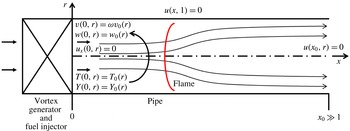
Schematic diagram of a premixed reacting swirling flow in an open pipe.

For a flow in a finite length, straight circular pipe of non-dimensional length
 $x_{0}$
, we consider the following boundary conditions; see the set-up in figure 1. At the pipe inlet,
 $x=0$
, the profiles of the axial velocity, the circumferential velocity, the axial derivative of radial velocity, the temperature and the mass fraction of the premixed reactant are fixed in time and are given respectively by
 $$\begin{eqnarray}\displaystyle & \displaystyle w(0,y)=w_{0}(y), & \displaystyle\end{eqnarray}$$
 $$\begin{eqnarray}\displaystyle & \displaystyle v(0,y)={\it\omega}v_{0}(y), & \displaystyle\end{eqnarray}$$
 $$\begin{eqnarray}\displaystyle & \displaystyle u_{x}(0,y)=0, & \displaystyle\end{eqnarray}$$
 $$\begin{eqnarray}\displaystyle & \displaystyle T(0,y)=T_{0}(y), & \displaystyle\end{eqnarray}$$
 $$\begin{eqnarray}\displaystyle & \displaystyle Y(0,y)=Y_{0}(y), & \displaystyle\end{eqnarray}$$
for
 $0\leqslant y\leqslant 1/2$
. Here,
 ${\it\omega}$
is the swirl ratio of the incoming flow. It is assumed that the inlet conditions are generated by a fuel injector with a vortex generator, that mixes fuel and oxidizer ahead of the pipe and is at a continuous and steady operation. Condition (2.40) allows a degree of freedom at the inlet to develop a radial velocity in order to model the upstream influence of propagating disturbances in the flow. The case with
 $u_{x}(0,y)\neq 0$
was studied in Rusak (Reference Rusak1998) and describes how general azimuthal vorticity profiles at the inlet can be included. The inlet conditions may represent the flow behind a vane guide vortex generator in a fuel injector as found in the experiments of Gupta et al. (Reference Gupta, Lilley and Syred1984, Reference Gupta, Lewis and Qi1998), Paschereit et al. (Reference Paschereit, Gutmark and Weisenstein1998) and Umeh et al. (Reference Umeh, Rusak and Gutmark2012). They are also common in numerical simulations of reacting flows with swirl (Grinstein & Fureby Reference Grinstein and Fureby2005; Grinstein et al.
Reference Grinstein, Liu and Oefelein2006; Choi et al.
Reference Choi, Rusak and Kapila2007).
The outlet flow is assumed to be in an
 $x$
-independent (parallel columnar) state at
 $x=x_{0}$
, i.e.
 $$\begin{eqnarray}{\it\Psi}_{x}(x_{0},y)=K_{x}(x_{0},y)=T_{x}(x_{0},y)=0\quad \text{for}~0\leqslant y\leqslant y_{0}.\end{eqnarray}$$
These outlet conditions are appropriate for a sufficiently long open pipe, where the flow downstream of the reaction zone settles naturally on a parallel (columnar) state ahead of the outlet, see experiments of Umeh et al. (Reference Umeh, Rusak and Gutmark2012) and numerical simulations of Choi et al. (Reference Choi, Rusak and Kapila2007).
Along the pipe centreline at
 $y=0$
, the axisymmetry assumption requires
 ${\it\Psi}(x,0)=0$
for
 $0\leqslant x\leqslant x_{0}$
. Along the pipe wall,
 $y=1/2$
, the no-penetration condition results in a constant
 ${\it\Psi}$
, i.e.
 $$\begin{eqnarray}{\it\Psi}(x,1/2)={\it\Psi}_{w}=\int _{0}^{1/2}{\it\rho}_{0}(\bar{y})w_{0}(\bar{y})\,\text{d}\bar{y}\quad \text{for}~0\leqslant x\leqslant x_{0}.\end{eqnarray}$$
The functions
 $K({\it\Psi})$
,
 $H({\it\Psi})$
and
 $s({\it\Psi})$
are defined in the range of
 $0\leqslant {\it\Psi}\leqslant {\it\Psi}_{w}$
. In addition, to accommodate possible solutions with separation zones, we assume that
 $$\begin{eqnarray}\displaystyle \left.\begin{array}{@{}c@{}}K({\it\Psi})=K(0)=0,\quad H({\it\Psi})=H(0)=H_{0},\quad s({\it\Psi})=s(0)=s_{0},\\ K^{\prime }({\it\Psi})=H^{\prime }({\it\Psi})=s^{\prime }({\it\Psi})=0,\end{array}\right\} & & \displaystyle\end{eqnarray}$$
when
 ${\it\Psi}<0$
, and
 $$\begin{eqnarray}\displaystyle \left.\begin{array}{@{}c@{}}K({\it\Psi})=K({\it\Psi}_{w})=K_{w},\quad H({\it\Psi})=H({\it\Psi}_{w})=H_{w},\quad s({\it\Psi})=s({\it\Psi}_{w})=s_{w},\\ K^{\prime }({\it\Psi})=H^{\prime }({\it\Psi})=s^{\prime }({\it\Psi})=0,\end{array}\right\} & & \displaystyle\end{eqnarray}$$
when
 ${\it\Psi}>{\it\Psi}_{w}$
. These assumptions have been used in Rusak & Wang (Reference Rusak and Wang2014), Rusak et al. (Reference Rusak, Choi, Bourquard and Wang2015) to describe vortex breakdown and wall separation zones in incompressible and compressible swirling flows.
For a sufficiently long pipe, the flow nature downstream of the thin reaction zone as described by the partial differential equation (PDE) (2.34) is dictated by the outlet state. Since the outlet is columnar and with no radial velocity, the flow becomes asymptotically columnar as the outlet is approached with zero reactant mass fraction.
3 The columnar state
In order to determine the possible outlet states of a low Mach number reacting swirling flow, we study the columnar state problem according to the governing PDE (2.34). A state is defined as columnar when the flow is
 $x$
-independent for all
 $x$
, i.e.
 $u=0$
, and
 ${\it\Psi}={\it\Psi}(y)$
.
We first determine the properties of a base non-reacting columnar state where
 $w=w_{0}(y)$
,
 $v={\it\omega}v_{0}(y)$
,
 $T=T_{0}(y)$
,
 $p=p_{0}(y)$
and
 ${\it\rho}={\it\rho}_{0}(y)$
according to the given inlet profiles. From the radial momentum equation for the columnar state,
 $p_{0r}={\it\gamma}Ma_{0}^{2}{\it\rho}_{0}({\it\omega}^{2}v_{0}^{2})/r$
. Together with the equation of state,
 $p_{0}={\it\rho}_{0}T_{0}$
, it is found that
 $p_{0y}/p_{0}={\it\gamma}Ma_{0}^{2}{\it\omega}^{2}({v_{0}}^{2}(y))/(2yT_{0}(y))$
. With the condition
 $p_{0}(0)=1$
, it is found that the base flow pressure and density profiles are
 $$\begin{eqnarray}\displaystyle & \displaystyle p_{0}(y)=\exp \left(\frac{{\it\gamma}Ma_{0}^{2}{\it\omega}^{2}}{2}\int _{0}^{y}\frac{{v_{0}}^{2}(\bar{y})}{\bar{y}T_{0}(\bar{y})}\,\text{d}\bar{y}\right), & \displaystyle\end{eqnarray}$$
 $$\begin{eqnarray}\displaystyle & \displaystyle {\it\rho}_{0}(y)=\frac{1}{T_{0}(y)}\exp \left(\frac{{\it\gamma}Ma_{0}^{2}{\it\omega}^{2}}{2}\int _{0}^{y}\frac{{v_{0}}^{2}(\bar{y})}{\bar{y}T_{0}(\bar{y})}\,\text{d}\bar{y}\right), & \displaystyle\end{eqnarray}$$
for
 $0\leqslant y\leqslant 1/2$
. Then, from
 ${\it\Psi}_{y}={\it\rho}w$
and the density profile (3.2), we can compute
 ${\it\Psi}_{0}(y)$
, i.e.
 $$\begin{eqnarray}{\it\Psi}_{0}(y)=\int _{0}^{y}{\it\rho}_{0}(\bar{y})w_{0}(\bar{y})\,\text{d}\bar{y},\end{eqnarray}$$
for
 $0\leqslant y\leqslant 1/2$
. Then,
 ${\it\Psi}_{w}={\it\Psi}_{0}(1/2)$
. Since
 ${\it\Psi}_{0}(y)$
is a monotonic increasing function, this function can be inverted such that
 $y=y({\it\Psi}_{0})$
for
 $0\leqslant {\it\Psi}\leqslant {\it\Psi}_{w}$
. Then, from the base circulation
 $K_{0}(y)={\it\omega}\sqrt{2y}v_{0}(y)$
, we find
 $$\begin{eqnarray}K_{0}({\it\Psi}_{0})={\it\omega}\sqrt{2y({\it\Psi}_{0})}v_{0}(y({\it\Psi}_{0})).\end{eqnarray}$$
From
 $H_{0}(y)=T_{0}(y)+(({\it\gamma}-1)Ma_{0}^{2})/2({\it\omega}^{2}{v_{0}}^{2}(y)+{w_{0}}^{2}(y))$
, we find
 $$\begin{eqnarray}H_{0}({\it\Psi}_{0})=T_{0}(y({\it\Psi}_{0}))+\frac{({\it\gamma}-1)Ma_{0}^{2}}{2}({\it\omega}^{2}{v_{0}}^{2}(y({\it\Psi}_{0}))+{w_{0}}^{2}(y({\it\Psi}_{0}))).\end{eqnarray}$$
Moreover, from
 $$\begin{eqnarray}\displaystyle & \displaystyle s_{0}(y)=\ln \left(\frac{T_{0}(y)}{({\it\rho}_{0}(y))^{{\it\gamma}-1}}\right)=\ln \left((T_{0}(y))^{{\it\gamma}}\left\{\exp \left[\frac{{\it\gamma}Ma_{0}^{2}{\it\omega}^{2}}{2}\int _{0}^{y}\frac{{v_{0}}^{2}(\bar{y})}{\bar{y}T_{0}(\bar{y})}\,\text{d}\bar{y}\right]\right\}^{-({\it\gamma}-1)}\right), & \displaystyle \nonumber\\ \displaystyle & & \displaystyle\end{eqnarray}$$
we find
 $$\begin{eqnarray}\displaystyle s_{0}({\it\Psi}_{0})={\it\gamma}\left[\ln (T_{0}(y({\it\Psi}_{0})))-\frac{({\it\gamma}-1)Ma_{0}^{2}{\it\omega}^{2}}{2}\int _{0}^{y({\it\Psi}_{0})}\frac{{v_{0}}^{2}(\bar{y})}{\bar{y}T_{0}(\bar{y})}\,\text{d}\bar{y}\right]. & & \displaystyle\end{eqnarray}$$
From the circulation, total enthalpy and entropy functions in terms of
 ${\it\Psi}$
, (3.4)–(3.7), the derivatives of these functions with respect to
 ${\it\Psi}$
are given by
 $$\begin{eqnarray}\displaystyle & \displaystyle K_{0}^{\prime }({\it\Psi}_{0})=\frac{\text{d}K}{\text{d}y}\frac{\text{d}y}{\text{d}{\it\Psi}}=\frac{{\it\omega}(\sqrt{2y}v_{0}(y))_{y}}{{\it\rho}_{0}(y)w_{0}(y)}=\frac{{\it\omega}\left[(\sqrt{2y}v_{0}(y))_{y}\right]_{y=y({\it\Psi}_{0})}T_{0}(y({\it\Psi}_{0}))}{w_{0}(y({\it\Psi}_{0}))\exp \left[{\displaystyle \frac{{\it\gamma}Ma_{0}^{2}{\it\omega}^{2}}{2}}\displaystyle \int _{0}^{y({\it\Psi}_{0})}{\displaystyle \frac{{v_{0}}^{2}(\bar{y})}{\bar{y}T_{0}(\bar{y})}}\,\text{d}\bar{y}\right]}, & \displaystyle\end{eqnarray}$$
 $$\begin{eqnarray}\displaystyle H_{0}^{\prime }({\it\Psi}_{0}) & = & \displaystyle \frac{\text{d}H_{0}}{\text{d}y}\frac{\text{d}y}{\text{d}{\it\Psi}}=\frac{T_{0y}+({\it\gamma}-1)Ma_{0}^{2}({\it\omega}^{2}v_{0}v_{0y}+w_{0}w_{0y})}{{\it\rho}_{0}(y)w_{0}(y)},\nonumber\\ \displaystyle & = & \displaystyle T_{0}(y({\it\Psi}_{0}))\frac{T_{0y}(y({\it\Psi}_{0}))+({\it\gamma}-1)Ma_{0}^{2}[{\it\omega}^{2}v_{0}(y({\it\Psi}_{0}))v_{0y}(y({\it\Psi}_{0}))+w_{0}(y({\it\Psi}_{0}))w_{0y}(y({\it\Psi}_{0}))]}{w_{0}(y({\it\Psi}_{0}))\exp \left[\displaystyle \frac{{\it\gamma}Ma_{0}^{2}{\it\omega}^{2}}{2}\int _{0}^{y({\it\Psi}_{0})}\displaystyle \frac{{v_{0}}^{2}(\bar{y})}{\bar{y}T_{0}(\bar{y})}\,\text{d}\bar{y}\right]},\nonumber\\ \displaystyle & & \displaystyle\end{eqnarray}$$
 $$\begin{eqnarray}\displaystyle & \displaystyle s_{0}^{\prime }({\it\Psi}_{0})=\frac{\text{d}s_{0}}{\text{d}y}\frac{\text{d}y}{\text{d}{\it\Psi}}=\frac{{\it\gamma}T_{0\bar{y}}(y({\it\Psi}_{0}))-{\it\gamma}({\it\gamma}-1)Ma_{0}^{2}{\it\omega}^{2}{\displaystyle \frac{{v_{0}}^{2}(y({\it\Psi}_{0}))}{2y({\it\Psi}_{0})}}}{w_{0}(y({\it\Psi}_{0}))\exp \left[{\displaystyle \frac{{\it\gamma}Ma_{0}^{2}{\it\omega}^{2}}{2}}\displaystyle \int _{0}^{y({\it\Psi}_{0})}\displaystyle \frac{{v_{0}}^{2}(\bar{y})}{\bar{y}T_{0}(\bar{y})}\,\text{d}\bar{y}\right]}. & \displaystyle\end{eqnarray}$$
Equations (3.4)–(3.10) define the functions
 $K_{0}({\it\Psi})$
,
 $K_{0}^{\prime }({\it\Psi})$
,
 $H_{0}({\it\Psi})$
,
 $H_{0}^{\prime }({\it\Psi})$
,
 $s_{0}({\it\Psi})$
and
 $s_{0}^{\prime }({\it\Psi})$
(by replacing
 ${\it\Psi}_{0}$
with
 ${\it\Psi}$
) for a base non-reacting columnar flow according to the given inlet profiles.
For a reacting flow in a open pipe, (3.4)–(3.10) formulate the properties of the inlet state, and these are the inlet functions defined in (2.22)–(2.25) for the flow upstream of the reaction zone. In addition,
 $Y_{0}({\it\Psi})=Y_{0}(y({\it\Psi}))$
and this defines the function
 $Y_{0}({\it\Psi})$
in determining the total head and the entropy at the outlet according to (2.28) and (2.30). Also,
 $T_{0}({\it\Psi})=T_{0}(y({\it\Psi}))$
and this defines the function
 $T_{0}({\it\Psi})$
in determining the entropy at the outlet according to (2.30).
The governing PDE (2.34) becomes in the columnar (
 $x$
-independent) case at the outlet of a reacting flow in an open pipe (which is sufficiently far downstream of the reaction zone),
 $$\begin{eqnarray}\displaystyle & \displaystyle ({\it\gamma}-1)Ma_{0}^{2}\frac{1}{{\it\rho}}\left(\frac{{\it\Psi}_{y}}{{\it\rho}}\right)_{y}=H^{\prime }({\it\Psi})-({\it\gamma}-1)Ma_{0}^{2}\frac{K({\it\Psi})K^{\prime }({\it\Psi})}{2y}-\frac{1}{{\it\gamma}}Ts^{\prime }({\it\Psi}), & \displaystyle\end{eqnarray}$$
 $$\begin{eqnarray}\displaystyle & \displaystyle T=H({\it\Psi})-\frac{({\it\gamma}-1)Ma_{0}^{2}}{2}\left(\left(\frac{{\it\Psi}_{y}}{{\it\rho}}\right)^{2}+\frac{K^{2}({\it\Psi})}{2y}\right), & \displaystyle\end{eqnarray}$$
 $$\begin{eqnarray}\displaystyle & \displaystyle {\it\rho}=\left(\frac{H({\it\Psi})-{\displaystyle \frac{\left({\it\gamma}-1\right)Ma_{0}^{2}}{2}}\left(w^{2}+{\displaystyle \frac{K^{2}({\it\Psi})}{2y}}\right)}{\exp (s({\it\Psi}))}\right)^{1/({\it\gamma}-1)}, & \displaystyle\end{eqnarray}$$
where the various functions of
 ${\it\Psi}$
are defined according to the outlet functions in (2.26)–(2.30).
To simplify the solution of the ordinary differential equation (ODE) (3.11), we use
 $w={\it\Psi}_{y}/{\it\rho}$
. Then, (3.11) is equivalent to the following system of two nonlinear first-order ODEs in terms of
 $w$
and
 ${\it\Psi}$
,
 $$\begin{eqnarray}\displaystyle & \displaystyle w_{y}=\frac{1}{({\it\gamma}-1)Ma_{0}^{2}}{\it\rho}\left(H^{\prime }({\it\Psi})-({\it\gamma}-1)Ma_{0}^{2}\frac{K({\it\Psi})K^{\prime }({\it\Psi})}{2y}-\frac{1}{{\it\gamma}}Ts^{\prime }({\it\Psi})\right), & \displaystyle\end{eqnarray}$$
 $$\begin{eqnarray}\displaystyle & \displaystyle {\it\Psi}_{y}={\it\rho}w, & \displaystyle\end{eqnarray}$$
with,
 $$\begin{eqnarray}\displaystyle & \displaystyle T=H({\it\Psi})-\frac{({\it\gamma}-1)Ma_{0}^{2}}{2}\left(w^{2}+\frac{K^{2}({\it\Psi})}{2y}\right), & \displaystyle\end{eqnarray}$$
 $$\begin{eqnarray}\displaystyle & \displaystyle {\it\rho}=\left(\frac{H({\it\Psi})-{\displaystyle \frac{({\it\gamma}-1)Ma_{0}^{2}}{2}}\left(w^{2}+\displaystyle \frac{K^{2}({\it\Psi})}{2y}\right)}{\exp (s({\it\Psi}))}\right)^{1/({\it\gamma}-1)}, & \displaystyle\end{eqnarray}$$
and with boundary conditions:
 $$\begin{eqnarray}{\it\Psi}(0)=0,\quad {\it\Psi}(1/2)={\it\Psi}_{w}=\int _{0}^{1/2}{\it\rho}_{0}(\bar{y})w_{0}(\bar{y})\,\text{d}\bar{y}.\end{eqnarray}$$
A trivial solution of the columnar flow problem (3.14) and (3.15) is
 $w=w_{0}(y)$
,
 $v={\it\omega}v_{0}(y)$
,
 $T=T_{0}(y)$
with
 $p=p_{0}(y)$
,
 ${\it\rho}={\it\rho}_{0}(y)$
,
 $Y=0$
and
 $s=0$
given by the base flow solution (3.3), i.e. the base non-reacting columnar flow. The work of Wang & Rusak (Reference Wang and Rusak1997) for incompressible inert swirling flows shows that additional solutions of the nonlinear columnar flow problem exist when the swirl ratio
 ${\it\omega}$
is greater than the critical
 ${\it\omega}_{0}$
. These include states with decelerated flow along the centreline and vortex breakdown states, which describe the flow at the pipe exit. It is expected that a similar situation occurs in the low Mach number reacting flow case, showing the existence of multiple solutions of the problem (3.14)–(3.17) with conditions (3.18) and the appearance of vortex breakdown states. The ODEs problem (3.14)–(3.18) is solved using a standard fourth-order Runge–Kutta integration scheme and iterations until the centreline and wall conditions are satisfied. In all the examples shown below, we use
 ${\it\gamma}=1.4$
and an inlet Mach number,
 $Ma_{0}=0.001$
.
4 Solution types
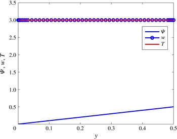
Similar to the incompressible flow case, the ODEs problem (3.14)–(3.18) may have several solution types, which describe the flow state at the pipe exit. We focus here on the type 0, type 1 and type 2 solutions relevant for a reacting flow in a straight pipe. The type 0 solution is the reacting flow at
 ${\it\omega}$
approaching 0. Figure 2 shows an example of the variation of
 ${\it\Psi}$
,
 $w$
and
 $T$
as a function of
 $y$
of the type 0 solution for an inlet solid-body rotation flow with constant unit axial velocity, constant unit temperature and constant reactant
 $Y_{0}={\it\delta}=0.043$
at
 ${\it\omega}=0$
and
 $Ma_{0}=0.001$
with
 ${\it\beta}{\it\delta}=2$
. In this solution, the flow properties are constant,
 $w=T=3$
,
 ${\it\rho}=1/3$
and
 ${\it\Psi}=y$
.
Example of the variation of
 ${\it\Psi}$
,
 $w$
and
 $T$
with
 $y$
of the type 0 solution of the ODE problem (3.14)–(3.18) at the pipe outlet. The inlet flow is the solid-body rotation with constant unit axial velocity and temperature at
 ${\it\omega}=0.001$
,
 $Ma_{0}=0.001$
and
 ${\it\beta}{\it\delta}=2$
.

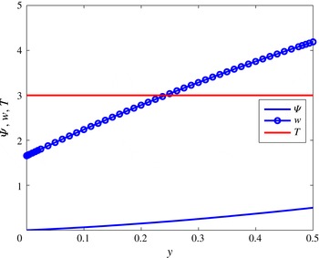
Type 1 solution of the ODEs system (3.14)–(3.18) is characterized by
 $0<w(0)<1+{\it\beta}{\it\delta}$
. In this type of solution,
 ${\it\Psi}(0)=0$
and iterations on
 $w(0)$
are repeated until the wall condition is satisfied. Figure 3 shows an example of the variation of
 ${\it\Psi}$
,
 $w$
and
 $T$
as a function of
 $y$
of the type 1 solution for an inlet solid-body rotation flow with constant unit axial velocity, constant unit temperature and constant reactant
 $Y_{0}={\it\delta}=0.043$
at
 ${\it\omega}=2.5$
and
 $Ma_{0}=0.001$
with
 ${\it\beta}{\it\delta}=2$
. In this solution,
 $w$
is decelerated near the centreline with respect to type 0 solution and accelerated near the wall. Also,
 $T\sim 3$
and
 ${\it\rho}\sim 1/3$
across the pipe and
 ${\it\Psi}$
is curved and monotonically increases.
Example of the variation of
 ${\it\Psi}$
,
 $w$
and
 $T$
with
 $y$
of the type 1 solution of the ODE problem (3.14)–(3.18) at the pipe outlet. The inlet flow is the solid-body rotation with constant unit axial velocity and temperature at
 ${\it\omega}=2.5$
,
 $Ma_{0}=0.001$
and
 ${\it\beta}{\it\delta}=2$
.

With further increase of swirl level
 ${\it\omega}$
, the flow along the centreline further decelerates until, at a certain swirl level
 ${\it\omega}_{0{\it\delta}}({\it\beta}{\it\delta})$
, the type 1 solution of the ODEs system (3.14)–(3.18) exhibits
 $w(0)=0$
. An approach to look for solutions with
 $w(0)<0$
is not relevant for the present case since under such a condition part of the outlet may become an inlet due to reversed axial flow. As a result, in searching for solutions that may represent the outlet state of the flow in the pipe, another type of solution is proposed when
 ${\it\omega}>{\it\omega}_{0{\it\delta}}$
. The type 2 solution is characterized by
 ${\it\Psi}=w=0$
and
 $T=1+{\it\beta}{\it\delta}$
in a finite range of
 $0\leqslant y\leqslant y_{s}$
. The value of
 $y_{s}$
is found by iterations until the solution develops from the point
 $y=y_{s}$
to the wall value of
 ${\it\Psi}(1/2)={\it\Psi}_{w}$
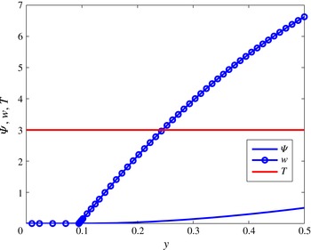
. Figure 4 shows an example of the variation of
 ${\it\Psi}$
,
 $w$
and
 $T$
as a function of
 $y$
of the type 2 solution for an inlet solid-body rotation flow with constant unit axial velocity, constant unit temperature and constant reactant
 $Y_{0}={\it\delta}=0.043$
at
 ${\it\omega}=4$
and
 $Ma_{0}=0.001$
with
 ${\it\beta}{\it\delta}=2$
. In this solution,
 $y_{s}=0.095$
(a radius of stagnation zone,
 $r_{s}=0.436$
) and
 $w$
increases in radial direction from 0 to 6.7 at the wall.
 ${\it\Psi}$
is 0 in the range of
 $0\leqslant y\leqslant y_{s}$
and is curved and monotonically increases outside of the stagnation zone.
Example of the variation of
 ${\it\Psi}$
,
 $w$
and
 $T$
with
 $y$
of the type 2 solution of the ODE problem (3.14)–(3.18) at the pipe outlet. The inlet flow is the solid-body rotation with constant unit axial velocity and temperature at
 ${\it\omega}=4$
,
 $Ma_{0}=0.001$
and
 ${\it\beta}{\it\delta}=2$
.

Similar three types of solutions are found for other inlet flow profiles, such as the Lamb–Oseen vortex with uniform axial velocity and temperature. These three types of solutions form the outlet states of the reacting flow in the open pipe.
5 Computed examples
In this section we focus on two representative cases where the inlet circumferential velocity is given by a solid-body rotation flow (§ 5.1) or by a Lamb–Oseen vortex model (§ 5.2). In both cases, we assume that the axial velocity and the temperature are constant. We derive the bifurcation diagrams of solutions of reacting swirling flows in a finite-length open pipe as the incoming flow swirl ratio is increased at various fixed exothermicity,
 ${\it\beta}{\it\delta}$
. In all cases,
 $Ma_{0}=0.001$
and
 ${\it\gamma}=1.4$
. Also,
 $Y_{0}={\it\delta}$
where
 $0\leqslant {\it\delta}<{\it\delta}_{st}$
and
 ${\it\delta}_{st}$
is the stoichiometric reactant mass fraction.
5.1 Solid-body rotation
Let the inlet flow describe a solid-body rotation with a constant unit axial velocity, constant unit temperature and constant inlet reactant mass fraction, i.e.
 $$\begin{eqnarray}\displaystyle v_{0}(y)=\sqrt{2y},\quad w_{0}(y)=T_{0}(y)=1,\quad Y_{0}(y)={\it\delta}\quad \text{for}~0\leqslant y\leqslant 1/2. & & \displaystyle\end{eqnarray}$$
Then, the base flow properties are
 $$\begin{eqnarray}\displaystyle & \displaystyle p_{0}(y)={\it\rho}_{0}(y)=\exp ({\it\gamma}Ma_{0}^{2}{\it\omega}^{2}y), & \displaystyle\end{eqnarray}$$
 $$\begin{eqnarray}\displaystyle & \displaystyle {\it\Psi}(y)=\frac{1}{{\it\gamma}Ma_{0}^{2}{\it\omega}^{2}}[\exp ({\it\gamma}Ma_{0}^{2}{\it\omega}^{2}y)-1], & \displaystyle\end{eqnarray}$$
 $$\begin{eqnarray}\displaystyle & \displaystyle {\it\Psi}_{w}={\it\Psi}(1/2)=\frac{1}{{\it\gamma}Ma_{0}^{2}{\it\omega}^{2}}\left[\exp \left(\frac{{\it\gamma}Ma_{0}^{2}{\it\omega}^{2}}{2}\right)-1\right], & \displaystyle\end{eqnarray}$$
 $$\begin{eqnarray}\displaystyle & \displaystyle y({\it\Psi})=\frac{1}{{\it\gamma}Ma_{0}^{2}{\it\omega}^{2}}\ln ({\it\gamma}Ma_{0}^{2}{\it\omega}^{2}{\it\Psi}+1). & \displaystyle\end{eqnarray}$$
From (3.4)–(3.10), we find
 $K_{0}({\it\Psi})$
,
 $K_{0}^{\prime }({\it\Psi})$
,
 $H_{0}({\it\Psi})$
,
 $H_{0}^{\prime }({\it\Psi})$
,
 $s_{0}({\it\Psi})$
and
 $s_{0}^{\prime }({\it\Psi})$
,
 $$\begin{eqnarray}\displaystyle & \displaystyle K_{0}({\it\Psi})=2{\it\omega}y({\it\Psi})=\frac{2}{{\it\gamma}Ma_{0}^{2}{\it\omega}}\ln ({\it\gamma}Ma_{0}^{2}{\it\omega}^{2}{\it\Psi}+1), & \displaystyle\end{eqnarray}$$
 $$\begin{eqnarray}\displaystyle & \displaystyle K_{0}^{\prime }({\it\Psi})=\frac{2{\it\omega}}{{\it\gamma}Ma_{0}^{2}{\it\omega}^{2}{\it\Psi}+1}, & \displaystyle\end{eqnarray}$$
 $$\begin{eqnarray}\displaystyle & \displaystyle H_{0}({\it\Psi})=1+\frac{({\it\gamma}-1)Ma_{0}^{2}}{2}\left(1+\frac{2}{{\it\gamma}Ma_{0}^{2}}\ln ({\it\gamma}Ma_{0}^{2}{\it\omega}^{2}{\it\Psi}+1)\right), & \displaystyle\end{eqnarray}$$
 $$\begin{eqnarray}\displaystyle & \displaystyle {H^{\prime }}_{0}({\it\Psi})=\frac{({\it\gamma}-1)Ma_{0}^{2}{\it\omega}^{2}}{({\it\gamma}Ma_{0}^{2}{\it\omega}^{2}{\it\Psi}+1)}, & \displaystyle\end{eqnarray}$$
 $$\begin{eqnarray}\displaystyle & \displaystyle s_{0}({\it\Psi})=-({\it\gamma}-1)\ln ({\it\gamma}Ma_{0}^{2}{\it\omega}^{2}{\it\Psi}+1), & \displaystyle\end{eqnarray}$$
 $$\begin{eqnarray}\displaystyle & \displaystyle {s^{\prime }}_{0}({\it\Psi})=-\frac{({\it\gamma}-1){\it\gamma}Ma_{0}^{2}{\it\omega}^{2}}{({\it\gamma}Ma_{0}^{2}{\it\omega}^{2}{\it\Psi}+1)}, & \displaystyle\end{eqnarray}$$
 $$\begin{eqnarray}\displaystyle & \displaystyle Y_{0}({\it\Psi})={\it\delta}. & \displaystyle\end{eqnarray}$$
To determine the outlet state, we use (2.28) and (2.29) to formulate the outlet functions
 $H({\it\Psi})$
and
 $s({\it\Psi})$
. Since in the present example the inlet reactant mass fraction is constant, we have
 $H^{\prime }({\it\Psi})={H^{\prime }}_{0}({\it\Psi})$
and
 $s^{\prime }({\it\Psi})={s^{\prime }}_{0}({\it\Psi})$
at the outlet. The effect of reaction appears only in computing
 $T$
and
 ${\it\rho}$
from
 $H({\it\Psi})$
and
 $s({\it\Psi})$
. Then, at the outlet, (3.14) and (3.15) become,
 $$\begin{eqnarray}\displaystyle & \displaystyle w_{y}={\it\rho}\frac{{\it\omega}^{2}}{({\it\gamma}Ma_{0}^{2}{\it\omega}^{2}{\it\Psi}+1)}\left(1+T-\frac{2}{{\it\gamma}Ma_{0}^{2}{\it\omega}^{2}y}\ln ({\it\gamma}Ma_{0}^{2}{\it\omega}^{2}{\it\Psi}+1)\right), & \displaystyle\end{eqnarray}$$
 $$\begin{eqnarray}\displaystyle & \displaystyle {\it\Psi}_{y}={\it\rho}w, & \displaystyle\end{eqnarray}$$
with
 $$\begin{eqnarray}\displaystyle T & = & \displaystyle 1+{\it\beta}{\it\delta}+\frac{({\it\gamma}-1)Ma_{0}^{2}}{2}\left\{\vphantom{\displaystyle \left(\frac{1}{{\it\gamma}Ma_{0}^{2}}\right)^{2}}1+\frac{2}{{\it\gamma}Ma_{0}^{2}}\ln ({\it\gamma}Ma_{0}^{2}{\it\omega}^{2}{\it\Psi}+1)\right.\nonumber\\ \displaystyle & & \displaystyle -\left.w^{2}-\frac{2{\it\omega}^{2}}{y}\left(\frac{1}{{\it\gamma}Ma_{0}^{2}{\it\omega}^{2}}\ln ({\it\gamma}Ma_{0}^{2}{\it\omega}^{2}{\it\Psi}+1)\right)^{2}\right\},\end{eqnarray}$$
 $$\begin{eqnarray}\displaystyle & \displaystyle {\it\rho}=T^{1/({\it\gamma}-1)}\frac{({\it\gamma}Ma_{0}^{2}{\it\omega}^{2}{\it\Psi}+1)}{(1+{\it\beta}{\it\delta})^{{\it\gamma}/({\it\gamma}-1)}}, & \displaystyle\end{eqnarray}$$
and with boundary conditions,
 $$\begin{eqnarray}{\it\Psi}(0)=0,\quad {\it\Psi}(1/2)={\it\Psi}_{w}=\frac{1}{{\it\gamma}Ma_{0}^{2}{\it\omega}^{2}}\left[\exp \left(\frac{{\it\gamma}Ma_{0}^{2}{\it\omega}^{2}}{2}\right)-1\right].\end{eqnarray}$$
We determine type 0, 1 and 2 solutions of system (5.13)–(5.17) in the range of
 $0\leqslant {\it\omega}\leqslant 4$
for various
 $0\leqslant {\it\beta}{\it\delta}\leqslant 2$
. Examples of these types of solutions are shown in figures 2–4.
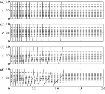
Contour plots of temperature (
 $T$
) and circulation (
 $K$
) for
 ${\it\beta}{\it\delta}=0.05$
with various
 ${\it\omega}$
: (a)
 ${\it\omega}=0.4$
, (b)
 ${\it\omega}=0.7$
, (c)
 ${\it\omega}=0.8$
, (d)
 ${\it\omega}=0.82$
. There are 15 equispaced lines of
 $T$
(solid lines) in the respective range [1, 1.05] and 15 equispaced lines of
 $K$
(dashed lines) in the respective range: (a) [0, 0.4], (b) [0, 0.69], (c) [0, 0.79], (d) [0, 0.81]. Here, the inlet flow is the Lamb–Oseen vortex with
 $b=4$
with unit axial velocity and temperature. Taken from Choi et al. (Reference Choi, Rusak and Kapila2007) with permission from Taylor & Francis Ltd., http://www.tandfonline.com.

Type 0 solution of the ODEs system (5.13)–(5.17) is the outlet state of a type 0 solution of the PDEs system (2.1)–(2.6) for zero swirl level. The type 0 solution of the PDE system describes a parallel flow in the pipe with zero swirl and a (classical) straight thin reaction zone across the pipe. The temperature increases due to the heat release across the reaction zone from an inlet value,
 $T(0,y)=1$
, to an outlet temperature,
 $T(x_{0},y)=1+{\it\beta}{\it\delta}$
. Thus, density decreases along the pipe. The position of reaction zone in the pipe is dictated by the reaction variables, activation energy
 ${\it\theta}$
and reaction rate
 $\mathscr{A}$
. Accordingly, from the continuity equation, the flow accelerates as a parallel flow across the reaction zone from an inlet axial velocity,
 $w(0,y)=1$
, to an outlet axial velocity,
 $w(x_{0},y)=1+{\it\beta}{\it\delta}$
. The numerical simulations in figure 5(a), taken from Choi et al. (Reference Choi, Rusak and Kapila2007), for
 ${\it\omega}\leqslant 0.4$
demonstrate an example of these flow and temperature patterns for a low swirl condition.
Type 1 solution of the ODEs system (5.13)–(5.17) is found in the range
 $0<{\it\omega}<{\it\omega}_{0{\it\delta}}({\it\beta}{\it\delta})$
and describes the outlet state of a type 1 solution of the PDEs system (2.1)–(2.6). Here,
 ${\it\omega}_{0{\it\delta}}$
is a critical swirl for the first appearance of breakdown states. In this solution, for a fixed heat release,
 ${\it\beta}{\it\delta}$
, the centreline outlet axial velocity
 $w(x_{0},0)<1+{\it\beta}{\it\delta}$
and decreases with increase of the inlet swirl,
 ${\it\omega}$
. This is the result of the increasing nonlinear interaction between convection of azimuthal vorticity and vorticity stretching related to axial gradient of the circulation which decreases azimuthal vorticity along the centreline, and thereby flow deceleration is increased, as also found in an inert flow. This mechanism is explained in details in Rusak et al. (Reference Rusak, Kapila and Choi2002) and also dominates reacting flows with swirl. By continuity, the wall outlet axial velocity
 $w(x_{0},1/2)>1+{\it\beta}{\it\delta}$
and increases with the increase of the inlet swirl,
 ${\it\omega}$
. As a result, we infer the structure of the flow and temperature in the pipe. The centreline axial velocity accelerates across the reaction zone from the inlet value
 $w(0,0)=1$
to
 $w=1+{\it\beta}{\it\delta}$
and then decelerates downstream of the reaction zone to the outlet axial velocity,
 $w(x_{0},0)<1+{\it\beta}{\it\delta}$
. Along the pipe wall, the axial velocity increases from the inlet value
 $w(0,1/2)=1$
to
 $1+{\it\beta}{\it\delta}$
at the reaction zone and to the outlet wall axial velocity of
 $w(x_{0},1/2)>1+{\it\beta}{\it\delta}$
. It is clear that the effect of incoming swirl is to decelerate the flow near the centreline and accelerate the flow along the wall. Therefore, the reaction zone is curved in the radial direction toward downstream, i.e. the reaction zone is pushed toward the inlet around the centreline and pushed downstream near the wall with respect to type 0 solution with no swirl. The temperature increases across the curved reaction zone from
 $T=1$
to an outlet temperature,
 $T=1+{\it\beta}{\it\delta}$
. The position of the reaction zone in the pipe is again dictated by the reaction variables,
 ${\it\theta}$
and
 $\mathscr{A}$
. The numerical simulations in figure 5(b,c), taken from Choi et al. (Reference Choi, Rusak and Kapila2007), for
 ${\it\omega}=0.7$
and 0.8 demonstrate these flow and temperature patterns for type 1 solutions.
With heat release from the reaction, flow is accelerated across the reaction zone. Then, with increase of heat release at a fixed inlet swirl level, type 1 solutions are also affected by the nonlinear interaction between convection of azimuthal vorticity and increased baroclinic effects resulting from the coupling between steepening temperature gradients and velocity gradients. This interaction makes a smaller decrease of azimuthal vorticity due to swirl near the centreline, and thereby the centreline outlet axial velocity is less decreased. These effects are also discussed in Rusak et al. (Reference Rusak, Kapila and Choi2002). The numerical simulations in figures 4(b) and 6(b) for
 ${\it\omega}=0.6$
in Choi et al. (Reference Choi, Rusak and Kapila2007) demonstrate these flow and temperature patterns.
Type 2 solution of the ODEs system (5.13)–(5.17) is found in the range
 ${\it\omega}>{\it\omega}_{0{\it\delta}}({\it\beta}{\it\delta})$
and forms the outlet state of a type 2 solution of the PDEs system (2.1)–(2.6), which describes a reacting swirling flow in the pipe with a finite size breakdown zone around the centreline. The width of the breakdown zone at the outlet is
 $y_{s}({\it\omega},{\it\beta}{\it\delta})$
. In such a flow state, for a fixed heat release, the nonlinear interactions between the convection of azimuthal vorticity and stretching of vorticity by axial gradient of circulation are stronger than in type 1 solutions and form the breakdown zone. The centreline axial velocity decelerates from the inlet value,
 $w(0,0)=1$
, to stagnation,
 $w=0$
, at a certain point along the centreline and remains zero from that point to the outlet. By continuity, along the pipe wall, the axial velocity increases from
 $w(0,1/2)=1$
to the outlet wall axial velocity of
 $w(x_{0},1/2)\gg 1+{\it\beta}{\it\delta}$
. Comparing figures 3 and 4, both at the same heat release
 ${\it\beta}{\it\delta}=2$
, it is clear that the effect of a high incoming swirl is to further decelerate the flow near the centreline and establish a centreline breakdown zone and to further accelerate the flow along the wall. Therefore, at higher incoming swirl levels, the reaction zone is much more curved in the radial direction toward downstream, i.e. the reaction zone is pushed further toward the inlet around the centreline and pushed further downstream near the wall. The temperature increases across the curved reaction zone from
 $T=1$
to an outlet temperature,
 $T=1+{\it\beta}{\it\delta}$
. The position of reaction zone in the pipe is again dictated by the reaction variables,
 ${\it\theta}$
and
 $\mathscr{A}$
. With increase of heat release at a fixed inlet swirl level, type 2 solutions also experience baroclinic effects, similar to those discussed above in type 1 solution. These effects delay the appearance of breakdown in the swirling reacting flow to higher swirl levels. The numerical simulations in figure 5(d) for
 ${\it\omega}=0.82$
demonstrate the flow and temperature patterns for type 2 solutions. In addition, figures 3–6 in Choi et al. (Reference Choi, Rusak and Kapila2007) for
 ${\it\omega}=0.86$
, 0.88 demonstrate the effect of increasing heat release on flow and temperature patterns of type 2 solutions. In all cases computed, the reaction zone is upstream of the leading stagnation point and wraps around the vortex breakdown separation zone. This is similar to flow and reaction zone patterns observed in the experimental study in figures 4 and 5 in Umeh et al. (Reference Umeh, Rusak and Gutmark2012).
We note that, in realistic situations, the velocity inside the breakdown zone is slightly negative due to viscous diffusion of momentum from the rotating bulk into the breakdown zone. The simulations of high Reynolds number inert flows show that the negative axial velocity inside the breakdown zone becomes smaller with increase of Reynolds number (Beran Reference Beran1994; Lopez Reference Lopez1994). In the inviscid limit case, it is expected that the zone becomes stagnant. This is supported by inviscid flow simulations which show natural evolution of perturbations in the flow to form a time-asymptotic near-stagnant breakdown zone (Rusak et al. Reference Rusak, Wang, Xu and Taylor2012).
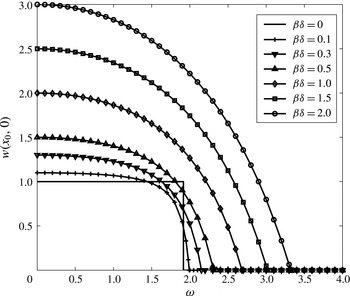
Bifurcation diagram of the outlet centreline axial velocity
 $w(x_{0},0)$
as a function of
 ${\it\omega}$
at various values of
 ${\it\beta}{\it\delta}$
for an inlet solid-body rotation flow with
 $Ma_{0}=0.001$
.

The ODEs system (5.13)–(5.17) is integrated numerically for a variety of values of
 ${\it\omega}$
and
 ${\it\beta}{\it\delta}$
with
 ${\it\gamma}=1.4$
and
 $Ma_{0}=0.001$
. The results of the computations are summarized in the bifurcation diagrams of solutions shown in figure 6. For a fixed
 ${\it\beta}{\it\delta}$
, the outlet centreline axial velocity
 $w(x_{0},0)=1+{\it\beta}{\it\delta}$
when
 ${\it\omega}=0$
, it decreases with increase of inlet swirl
 ${\it\omega}$
and becomes zero at the critical swirl level,
 ${\it\omega}_{0{\it\delta}}$
. For higher swirl,
 ${\it\omega}>{\it\omega}_{0{\it\delta}}$
, the outlet centreline axial velocity is zero. As the heat release,
 ${\it\beta}{\it\delta}$
, increases from zero, the outlet centreline axial velocity
 $w(x_{0},0)$
increases for a fixed inlet swirl in the range
 $0\leqslant {\it\omega}<{\it\omega}_{0{\it\delta}}$
. The first appearance of a vortex breakdown state is delayed with the increase of
 ${\it\beta}{\it\delta}$
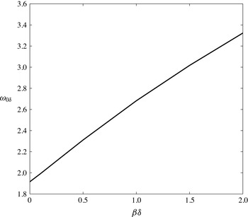
. Figure 7 shows the change of
 ${\it\omega}_{0{\it\delta}}$
with
 ${\it\beta}{\it\delta}$
at
 $Ma_{0}=0.001$
. It shows that the critical swirl for the first appearance of breakdown in the reacting flow increases monotonically with
 ${\it\beta}{\it\delta}$
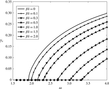
. The size,
 $y_{s}$
, of the breakdown zone at the outlet as a function of
 ${\it\omega}>{\it\omega}_{0{\it\delta}}$
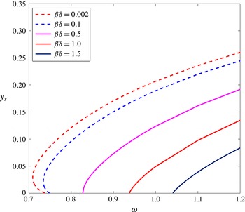
is shown in figure 8 for various
 ${\it\beta}{\it\delta}$
. The size
 $y_{s}$
increases with
 ${\it\omega}$
at a fixed
 ${\it\beta}{\it\delta}$
as a result of increased vorticity stretching related to the axial gradient of circulation. It decreases with increase of
 ${\it\beta}{\it\delta}$
at a fixed
 ${\it\omega}$
as a result of increased baroclinic effects related to axial temperature gradient. This variation of
 $y_{s}$
is a result of the swirl difference
 ${\it\omega}-{\it\omega}_{0{\it\delta}}$
. Since
 ${\it\omega}_{0{\it\delta}}$
increases with heat release, for a given swirl level, this swirl difference becomes smaller, making the breakdown zone smaller in size at the outlet and all over in the domain. We also observe in figure 6 the nonlinear interaction between the azimuthal vorticity stretching by axial gradient of temperature and the baroclinic terms at swirl level around
 ${\it\omega}=1.916$
(the critical swirl level for the non-reacting flow) for low amount of exothermicity
 $0<{\it\beta}{\it\delta}<0.5$
. This nonlinear interaction was predicted in the discussion in Choi et al. (Reference Choi, Rusak and Kapila2007). It is manifested by the results that
 $w(x_{0},0)$
is less than unity around the critical swirl and first decreases when heat release,
 ${\it\beta}{\it\delta}$
, is increased from 0 to around 0.1 and then increases as
 ${\it\beta}{\it\delta}$
increases from around 0.1 to 0.5.
Variation of the critical swirl
 ${\it\omega}_{0{\it\delta}}$
as a function of
 ${\it\beta}{\it\delta}$
for an inlet solid-body rotation flow with
 $Ma_{0}=0.001$
.

Variation of stagnation zone size,
 $y_{s}$
, at the pipe outlet as a function of
 ${\it\omega}$
at various
 ${\it\beta}{\it\delta}$
for an inlet solid-body rotation flow with
 $Ma_{0}=0.001$
.

5.2 Lamb–Oseen vortex model
Let the inlet flow describe a Lamb–Oseen vortex with a uniform axial speed, uniform temperature and constant inlet reactant mass fraction, i.e.
 $$\begin{eqnarray}v_{0}(y)=\frac{1}{\sqrt{2y}}(1-\exp (-2by)),\quad w_{0}(y)=T_{0}(y)=1,\quad Y_{0}(y)={\it\delta},\quad \text{for}~0\leqslant y\leqslant 1/2.\end{eqnarray}$$
Here,
 $b$
is the vortex core size parameter where the vortex core radius is
 $r_{c}=1.12/\sqrt{b}$
. Then, the base flow pressure obeys
 $p_{0y}={\it\gamma}Ma_{0}^{2}{\it\omega}^{2}p_{0}({v_{0}}^{2}(y))/(2yT_{0}(y))={\it\gamma}Ma_{0}^{2}{\it\omega}^{2}p_{0}((1-\exp (-2by))^{2})/4y^{2}$
with centreline condition
 $p_{0}(0)=1$
. This equation can be integrated numerically to determine
 $p_{0}(y)$
. Since the base flow temperature is
 $T_{0}(y)=1$
, the base flow density is
 ${\it\rho}_{0}(y)=p_{0}(y)$
. Then, the base flow stream function obeys
 ${\it\Psi}_{0y}=p_{0}(y)$
with
 ${\it\Psi}_{0}(0)=0$
, and
 ${\it\Psi}_{0}(y)=\int _{0}^{y}p_{0}(\bar{y})\,\text{d}\bar{y}$
. This equation can again be integrated numerically in the range
 $0\leqslant y\leqslant 1/2$
. Therefore,
 ${\it\Psi}_{w}={\it\Psi}_{0}(1/2)$
. The function
 ${\it\Psi}_{0}(y)$
is monotonically increasing and can be inverted to give
 $y({\it\Psi}_{0})$
. Using a curve fit formula, a ninth-order polynomial expansion for
 $y({\it\Psi}_{0})$
at every
 ${\it\omega}$
was determined. Then, replacing
 ${\it\Psi}_{0}$
with
 ${\it\Psi}$
, it is found that,
 $$\begin{eqnarray}\displaystyle & \displaystyle K_{0}({\it\Psi})={\it\omega}(1-\exp (-2by({\it\Psi}))), & \displaystyle\end{eqnarray}$$
 $$\begin{eqnarray}\displaystyle & \displaystyle K_{0}^{\prime }({\it\Psi})=\frac{2b{\it\omega}\exp (-2by({\it\Psi}))}{p_{0}(y({\it\Psi}))}, & \displaystyle\end{eqnarray}$$
 $$\begin{eqnarray}\displaystyle & \displaystyle H_{0}({\it\Psi})=1+\frac{({\it\gamma}-1)Ma_{0}^{2}}{2}\left(1+\frac{{\it\omega}^{2}}{2y({\it\Psi})}[1-\exp (-2by({\it\Psi}))]^{2}\right), & \displaystyle\end{eqnarray}$$
 $$\begin{eqnarray}\displaystyle & \displaystyle H_{0}^{\prime }({\it\Psi})=\frac{({\it\gamma}-1)Ma_{0}^{2}{\it\omega}^{2}v_{0}(y({\it\Psi}))v_{0y}(y({\it\Psi}))}{p_{0}(y({\it\Psi}))}, & \displaystyle\end{eqnarray}$$
 $$\begin{eqnarray}\displaystyle & \displaystyle s_{0}({\it\Psi})=-\frac{{\it\gamma}({\it\gamma}-1)Ma_{0}^{2}{\it\omega}^{2}}{2}\int _{0}^{y({\it\Psi})}\frac{(1-\exp (-2b\bar{y}))^{2}}{2\bar{y}^{2}}\,\text{d}\bar{y} & \displaystyle\end{eqnarray}$$
 $$\begin{eqnarray}\displaystyle & \displaystyle s_{0}^{\prime }({\it\Psi})=-\frac{{\it\gamma}({\it\gamma}-1)Ma_{0}^{2}{\it\omega}^{2}(1-\exp (-2by({\it\Psi})))^{2}}{4y^{2}({\it\Psi})p_{0}(y({\it\Psi}))}. & \displaystyle\end{eqnarray}$$
To determine the outlet state, we use total enthalpy and entropy equations, (2.28) and (2.29), to formulate the outlet functions
 $H({\it\Psi})$
and
 $s({\it\Psi})$
. Since in the present example the inlet reactant mass fraction is constant,
 $H^{\prime }({\it\Psi})=H_{0}^{\prime }({\it\Psi})$
and
 $s^{\prime }({\it\Psi})=s_{0}^{\prime }({\it\Psi})$
. The effect of reaction appears only in computing
 $T$
and
 ${\it\rho}$
from
 $H({\it\Psi})$
and
 $s({\it\Psi})$
. Then, at the outlet, the simplified ODEs (3.14) and (3.15), temperature and density become
 $$\begin{eqnarray}\displaystyle & \displaystyle w_{y}=\frac{1}{({\it\gamma}-1)Ma_{0}^{2}}{\it\rho}\left({H^{\prime }}_{0}({\it\Psi})-({\it\gamma}-1)Ma_{0}^{2}\frac{K({\it\Psi})K^{\prime }({\it\Psi})}{2y}-\frac{1}{{\it\gamma}}T{s^{\prime }}_{0}({\it\Psi})\right), & \displaystyle\end{eqnarray}$$
 $$\begin{eqnarray}\displaystyle & \displaystyle {\it\Psi}_{y}={\it\rho}w, & \displaystyle\end{eqnarray}$$
 $$\begin{eqnarray}\displaystyle & \displaystyle T=H_{0}({\it\Psi})-\frac{({\it\gamma}-1)Ma_{0}^{2}}{2}\left(w^{2}+\frac{K^{2}({\it\Psi})}{2y}\right)+{\it\beta}{\it\delta}, & \displaystyle\end{eqnarray}$$
 $$\begin{eqnarray}\displaystyle & \displaystyle {\it\rho}=\left(\frac{H_{0}({\it\Psi})-{\displaystyle \frac{({\it\gamma}-1)Ma_{0}^{2}}{2}}\left(w^{2}+{\displaystyle \frac{K^{2}({\it\Psi})}{2y}}\right)+{\it\beta}{\it\delta}}{\exp (s_{0}({\it\Psi}))(1+{\it\beta}{\it\delta})^{{\it\gamma}}}\right)^{1/({\it\gamma}-1)}, & \displaystyle\end{eqnarray}$$
and with boundary conditions,
 $$\begin{eqnarray}{\it\Psi}(0)=0,\quad {\it\Psi}(1/2)={\it\Psi}_{w}=\int _{0}^{1/2}p_{0}(\overline{y})\,\text{d}\overline{y}.\end{eqnarray}$$
In the present example, we focus on an inlet vortex with core size parameter
 $b=4$
(
 $r_{c}=0.56$
). Solutions similar to the type 0 (at
 ${\it\omega}=0$
), 1 and 2 of the solid-body rotation case are also found in this case. Numerically computed examples from Choi et al. (Reference Choi, Rusak and Kapila2007) of flow and temperature patterns for type 1 reacting flow solutions are shown in figure 5(a–c), and an example of these patterns for a type 2 reacting flow solution is shown in figure 5(d). However, the manifold of solutions for the Lamb–Oseen inlet vortex is more complicated and exhibits nonlinearity as the heat release,
 ${\it\beta}{\it\delta}$
, is increased. The bifurcation diagrams of the outlet centreline axial velocity,
 $w(x_{0},0)$
, as a function of the inlet swirl level,
 ${\it\omega}$
, for various small values of
 ${\it\beta}{\it\delta}$
in the range
 $0<{\it\beta}{\it\delta}\leqslant 0.2$
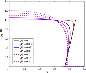
are first studied and shown in figure 9. For the inert flow case of
 ${\it\beta}{\it\delta}=0$
, the base type 0 flow is a solution of the problem for all inlet swirl level,
 ${\it\omega}$
, and the outlet centreline axial velocity is constant,
 $w(x_{0},0)=1$
for all
 ${\it\omega}$
. There is a transcritical bifurcation of type 1 non-columnar decelerated flow states along the centreline with
 $0<w(x_{0},0)<1$
as
 ${\it\omega}$
is decreased from a critical swirl level
 ${\it\omega}_{1}=0.882$
to
 ${\it\omega}=0.74$
, see the solid black line in figure 9. With respect to the solid-body rotation, the critical swirl level decreases with reduction of core size. This is consistent with Rusak et al. (Reference Rusak, Whiting and Wang1998). Type 2 states appear as the inlet swirl level,
 ${\it\omega}$
, is further decreased from 0.74 to a second critical swirl level
 ${\it\omega}_{0}=0.71$
. At
 ${\it\omega}_{0}=0.71$
, the type 2 solutions fold and develop with the increase of
 ${\it\omega}$
above
 ${\it\omega}_{0}=0.71$
.
Bifurcation diagram of the outlet centreline axial velocity
 $w(x_{0},0)$
as a function of
 ${\it\omega}$
at various values of
 $0\leqslant {\it\beta}{\it\delta}\leqslant 0.2$
for an inlet Lamb–Oseen vortex with
 $b=4$
and
 $Ma_{0}=0.001$
.

With a small increase of heat release,
 ${\it\beta}{\it\delta}$
, from 0 to 0.002, the transcritical bifurcation of solutions is modified into one branch of type 1 solutions that starts at
 ${\it\omega}=0$
with the outlet centreline axial velocity of
 $w(x_{0},0)=1.002$
. The value of
 $w(x_{0},0)$
of this branch decreases with the increase of
 ${\it\omega}$
up to a modified critical swirl level
 ${\it\omega}_{1{\it\delta}}=0.86$
. The branch folds at
 ${\it\omega}_{1{\it\delta}}=0.86$
and
 $w(x_{0},0)$
decreases with the decrease of
 ${\it\omega}$
down to 0.74. A branch of type 2 solutions develops between 0.74 and a second modified critical swirl level
 ${\it\omega}_{0{\it\delta}}=0.71$
and then folds to form breakdown states as
 ${\it\omega}$
increases above
 ${\it\omega}_{0{\it\delta}}$
. Further increase of
 ${\it\beta}{\it\delta}$
up to 0.2 results in similar behaviour, but with the decrease of the first fold point
 ${\it\omega}_{1{\it\delta}}$
and the increase of the second fold point
 ${\it\omega}_{0{\it\delta}}$
. At
 ${\it\beta}{\it\delta}=0.15$
,
 ${\it\omega}_{1{\it\delta}}$
achieves a minimum value with increase of heat release,
 ${\it\beta}{\it\delta}$
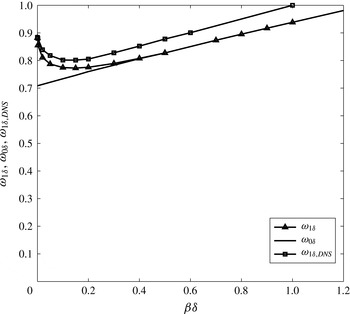
. This result is supported by the asymptotic analysis of Rusak et al. (Reference Rusak, Kapila and Choi2002) for weak reaction in swirling flows. In this range of relatively small heat release, the flow is dominated by the interaction between the convection of azimuthal vorticity and the stretching of vorticity by axial gradient of circulation. The small heat release creates small baroclinic effects due to the coupling between the small axial temperature gradient and the circulation. These effects support the flow mechanism of reduction of azimuthal vorticity along the centreline to form a decelerated flow at lower swirl levels and a transition to breakdown at a lower critical swirl level with respect to the inert flow.
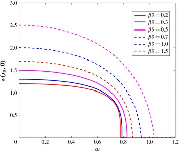
The bifurcation diagrams of the outlet centreline axial velocity,
 $w(x_{0},0)$
, as a function of the inlet swirl,
 ${\it\omega}$
, for larger values of heat release,
 ${\it\beta}{\it\delta}>0.2$
, are shown in figure 10. At
 ${\it\beta}{\it\delta}=0.4$
, we find that
 ${\it\omega}_{1{\it\delta}}={\it\omega}_{0{\it\delta}}$
, and the fold behaviour of the branch of solutions disappears with increase of heat release,
 ${\it\beta}{\it\delta}$
, above 0.4, i.e. for a fixed
 ${\it\beta}{\it\delta}$
,
 $w(x_{0},0)$
develops as one uniform branch and breakdown appears when
 ${\it\omega}>{\it\omega}_{0{\it\delta}}$
. The values of
 $w(x_{0},0)$
in the range
 $0\leqslant {\it\omega}\leqslant {\it\omega}_{0{\it\delta}}$
increase monotonically with increase of
 ${\it\beta}{\it\delta}$
at a fixed
 ${\it\omega}$
. We find that the first appearance of vortex breakdown zone is delayed with increase of
 ${\it\beta}{\it\delta}$
. This result is supported by the discussion in Choi et al. (Reference Choi, Rusak and Kapila2007) on reacting swirling flows. In this range of higher heat release, the flow is dominated by the interaction between the convection of azimuthal vorticity and the stretching of vorticity by axial gradient of circulation. The higher values of heat release create large baroclinic effects due to the coupling between the gradients of temperature and the gradients of the axial and radial velocities. These effects overcome the baroclinic term due to the coupling between axial temperature gradient and circulation. Thereby, the net baroclinic effects make a smaller decrease of the azimuthal vorticity, which results in the axial flow acceleration with respect to case with
 ${\it\beta}{\it\delta}<0.15$
, and the increase of the first critical swirl with increase of heat release above 0.15.
Bifurcation diagram of the outlet centreline axial velocity
 $w(x_{0},0)$
as a function of
 ${\it\omega}$
at various values of
 ${\it\beta}{\it\delta}\geqslant 0.2$
for an inlet Lamb–Oseen vortex with
 $b=4$
and
 $Ma_{0}=0.001$
.

The size,
 $y_{s}$
, of the breakdown zone at the outlet as a function of the inlet swirl level,
 ${\it\omega}$
, and for various heat release,
 ${\it\beta}{\it\delta}$
, is described in figure 11. For small
 ${\it\beta}{\it\delta}$
between 0 and 0.4, the lines of
 $y_{s}$
first increase with the decrease of
 ${\it\omega}$
. This corresponds to the appearance of small breakdown zones as swirl is decreased from 0.74 to
 ${\it\omega}_{0{\it\delta}}$
. The lines of
 $y_{s}$
fold at
 ${\it\omega}_{0{\it\delta}}$
and continue to increase with
 ${\it\omega}>{\it\omega}_{0{\it\delta}}$
. This part of lines corresponds to the appearance of larger breakdown zones as swirl is increased above
 ${\it\omega}_{0{\it\delta}}$
. However, for higher values of heat release,
 ${\it\beta}{\it\delta}>0.4$
, the lines monotonically increase as
 ${\it\omega}$
increases above
 ${\it\omega}_{0{\it\delta}}$
. This corresponds to the disappearance of the fold behaviour in the bifurcation diagram when
 ${\it\beta}{\it\delta}>0.4$
. We also find that the breakdown zone size,
 $y_{s}$
, at the outlet decreases with the increase of heat release,
 ${\it\beta}{\it\delta}$
, at a fixed inlet swirl level,
 ${\it\omega}$
. This behaviour of
 $y_{s}$
is dominated by the interaction between convection of azimuthal vorticity, vorticity stretching by circulation gradients and various baroclinic effects as mentioned above.
Variation of stagnation zone size,
 $y_{s}$
, at the pipe outlet as a function of
 ${\it\omega}$
at various
 ${\it\beta}{\it\delta}$
for an inlet Lamb–Oseen vortex with
 $b=4$
and
 $Ma_{0}=0.001$
.

Variation of critical swirls,
 ${\it\omega}_{0{\it\delta}}$
(solid line) and
 ${\it\omega}_{1{\it\delta}}$
(line with filled triangles), as a function of
 ${\it\beta}{\it\delta}$
for an inlet Lamb–Oseen vortex with
 $b=4$
and
 $Ma_{0}=0.001$
.

The variation of the first critical swirl level,
 ${\it\omega}_{1{\it\delta}}$
, (line with filled triangles) and of the second critical swirl level,
 ${\it\omega}_{0{\it\delta}}$
, (solid line) with heat release,
 ${\it\beta}{\it\delta}$
, for the Lamb–Oseen inlet vortex with
 $b=4$
are shown in figure 12. It can be seen that for small values of
 ${\it\beta}{\it\delta}$
,
 ${\it\omega}_{1{\it\delta}}$
decreases and
 ${\it\omega}_{0{\it\delta}}$
increases with increase of
 ${\it\beta}{\it\delta}$
. However, once
 ${\it\beta}{\it\delta}$
is increased beyond a certain level of about 0.4,
 ${\it\omega}_{0{\it\delta}}$
coincides with
 ${\it\omega}_{1{\it\delta}}$
and only
 ${\it\omega}_{0{\it\delta}}$
exists and increases with further increase of
 ${\it\beta}{\it\delta}$
. This indicates again that fold behaviour exists only for small values of heat release and disappears for larger values. Also shown in figure 12 are the results of numerical simulations from Choi et al. (Reference Choi, Rusak and Kapila2007) for the first appearance of vortex breakdown in premixed reacting flows in a straight open pipe (line with filled squares). In the numerical simulation, the inlet flow is also given by the Lamb–Oseen vortex with
 $b=4$
. It is understood now that the transition to breakdown in the simulations at low values of
 ${\it\beta}{\it\delta}$
below 0.4 is related to the jump of solutions from a near-columnar state to a breakdown state when swirl was increased from below to above the first critical value at
 ${\it\omega}_{1{\it\delta}}({\it\beta}{\it\delta})$
. On the other hand, the appearance of breakdown in the simulations at high values of
 ${\it\beta}{\it\delta}$
above 0.4 is related to the gradual change of nature of the states when swirl level increases above
 ${\it\omega}_{0{\it\delta}}({\it\beta}{\it\delta})$
. The computed results from the present approach capture the major trend of the nonlinear behaviour predicted by the numerical simulations of Choi et al. (Reference Choi, Rusak and Kapila2007) although the numerical results differ by small amount of swirl. This difference can be explained by the possible effect of pipe length. The present study assumes a relatively long pipe such that a fully developed columnar state is established ahead of the outlet. On the other hand, the numerical simulations used a relatively short pipe of two radii length. It is known from the inert flow simulations of Rusak et al. (Reference Rusak, Whiting and Wang1998) that pipe length increases the critical swirl level for vortex breakdown from
 ${\it\omega}_{0}$
by an amount that is inversely proportional to the pipe length. Specifically for short pipes that amount of increase is not negligible and creates a finite small difference between the predicted line by the present approach and the numerical simulation results.
6 Conclusions
The global properties of steady states of low Mach number inviscid premixed reacting swirling flows in a straight finite-length open circular pipe is studied using global analysis techniques. The model considers a flow in a pipe that is generated by a fuel injector with a vortex generator ahead of the pipe at a continuous and steady operation (see figure 1). For analytical simplicity of describing the interaction between the swirling flow dynamics and heat release of the reaction, the present study focuses on a one-step first-order Arrhenious reaction kinetics at the high activation energy and infinite Peclet number. The analysis of the reacting flow equations shows that, when a complete reaction with chemical equilibrium is assumed downstream of the reaction zone, the flow downstream of the reaction zone is described by a nonlinear PDE (2.34) for the solution of the flow stream function in terms of specific total enthalpy for a reacting flow, specific entropy and circulation functions that are prescribed at the inlet. Three types of solutions of the nonlinear ODE for the parallel (columnar) flow, that results from the PDE, are found and describe the outlet state of the solution of the PDE for a reacting flow with swirl in a sufficiently long open pipe. These solutions are used to form the bifurcation diagram of steady low Mach number flows with swirl and reaction as the inlet swirl level is increased at a fixed inlet Mach number and at a fixed heat release from the reaction. The PDE problem exhibits several types of solutions, the base parallel reacting flow without swirl with a straight normal reaction zone, the decelerating flow along the centreline with a curved reaction zone for the inlet swirl level in the range
 $0<{\it\omega}<{\it\omega}_{0{\it\delta}}$
(see figure 5
a–c) and the reacting flow with swirl and vortex breakdown when the inlet swirl level
 ${\it\omega}>{\it\omega}_{0{\it\delta}}$
(see figure 5
d). The approach is applied to two profiles of inlet flows, solid-body rotation and the Lamb–Oseen vortex, both with constant profiles of the axial velocity, temperature and mixture reactant mass fraction, see the bifurcation diagrams in figures 6, 9 and 10. The computed results provide for each case theoretical predictions of the critical swirl levels for the appearance of vortex breakdown states and of the size of the breakdown zone as a function of the inlet swirl ratio, Mach number and heat release of the reaction, see figures 7, 8, 11 and 12.
The analysis sheds light on the global dynamics of low Mach number reacting flows with swirl and vortex breakdown and on the interaction between vortex breakdown and the heat release that affects the shape and location of the reaction zone. For the inlet solid-body rotation flow, there is only one branch of solutions where flow is decelerated to breakdown as the inlet swirl is increased, and there is a delay in the appearance of breakdown with the increase of the heat release. For the inlet Lamb–Oseen vortex at low values of heat release, the branch of solutions exhibits two critical fold points, the first critical swirl level,
 ${\it\omega}_{1{\it\delta}}$
, and the second critical swirl level,
 ${\it\omega}_{0{\it\delta}}$
, and three solutions in the range of swirl between these critical points. At high values of heat release above a certain minimum value, there is again only one branch of solutions where the flow is decelerated to breakdown as inlet swirl is increased, and the appearance of breakdown is delayed with the increase of heat release. In both cases, we infer that the appearance of flow deceleration and vortex breakdown around the centreline and of flow acceleration along the wall with the increase of inlet swirl affects the shape of reaction zone. The reaction zone is pushed toward the inlet around the centreline and pushed downstream near the wall with the increase of inlet swirl at a fixed heat release. On the other hand, when the heat release is increased at a fixed inlet swirl, the breakdown zone is decreased in size and pushed downstream, and may even disappear. For lean reaction, the reaction zone moves upstream with increase of reactant mass fraction,
 ${\it\delta}$
. The computed results from the present approach capture the major trends of the nonlinear behaviour predicted in the numerical simulations of Choi et al. (Reference Choi, Rusak and Kapila2007). The results are also supported by the detailed discussions in Rusak et al. (Reference Rusak, Kapila and Choi2002) and Umeh et al. (Reference Umeh, Rusak and Gutmark2012). These discussions emphasize the interactions between flow dynamics and reaction as manifested by the interaction between flow convection, vorticity stretching and baroclinic effects.
In the present analysis, we focus on the case of a flow without viscosity, diffusion of species and heat conduction. The swirl level determines the size of the breakdown zone, which in turn changes the radial and axial velocities in the domain and affects the reaction zone shape. In realistic situations, viscosity, species diffusion and heat conduction always appear and thereby, swirl may affect heat release from the reaction and the shape of reaction zone not only through the size of the breakdown.
The methodology developed in this paper provides an analytical approach for the global properties of reacting flow states with swirl. Using the inlet and outlet states predicted in the paper, base steady and axisymmetric states can be constructed and the stability of these states in response to both axisymmetric and three dimensional global perturbations under the same boundary conditions can be studied. The approach can be also extended to include pipe divergence and contraction, that are typical of combustor geometries.