1 Introduction
Mixing of high-pressure (high-
 $p$
) multispecies in turbulent flows occurs in practical engineering applications that span the fields of the chemical, automotive and aerospace industries; there are also examples of such processes in planetary science, with the Venus lower atmosphere being a prominent example. High-
 $p$
turbulent reactive flows are a subset of these practical and scientific applications, and are encountered in diesel, gas turbine and liquid rocket engines; in many of these devices, the pressure of the combustion chamber is above the critical pressure of the fuel and/or the oxidizer (Masi et al.
Reference Masi, Bellan, Harstad and Okong’o2013). The fuel, being a mixture of species, may have several critical points. A critical point is defined in the thermodynamic phase space by the location where the compositions and densities of the coexisting phases are the same; the value of
 $p$
corresponding to a critical point is defined as a critical pressure,
 $p_{c}$
. Determination of the critical properties of a practical fuel, whether experimentally or theoretically, is a very challenging task (Lin & Tavlarides Reference Lin and Tavlarides2012), and therefore there is only scant information on this subject. Lin & Tavlarides (Reference Lin and Tavlarides2012) describe several correlations for computing the critical points of complex mixtures and report critical points for several diesel surrogates (from single-species surrogates to twelve-species surrogates) that are in the range of 550 K–750 K for the critical temperature,
 $T_{c},$
and in the range of 1.5 MPa–4 MPa for
 $p_{c}$
. Additionally, Lin & Tavlarides (Reference Lin and Tavlarides2012) report (
 $T_{c},p_{c}$
) estimates for two diesel fuels, with
 $T_{c}\in [720~\text{K},750~\text{K}]$
and
 $p_{c}\in [1.75~\text{MPa},2.25~\text{MPa}]$
; the prevailing equivalent conditions in diesel-engine chambers at the time of fuel injection exceed the largest values in these ranges of (
 $T_{c},p_{c}$
). For aviation fuels, Yu & Eser (Reference Yu and Eser1995) either measured
 $T_{c}$
or computed (
 $T_{c},p_{c}$
) using correlations:
 $T_{c}\in [650~\text{K},673~\text{K}]$
and
 $p_{c}\in [2.3~\text{MPa},3.4~\text{MPa}]$
, and this information indicates that (
 $T_{c},p_{c}$
) have smaller values than the corresponding conditions in gas turbine engine combustion chambers at fuel-injection time.
To control combustion in the chambers of these engines, one must control the processes of fuel penetration, mixing of reactants and timing of ignition; these are all unsteady processes. The actual control very much depends on the thermodynamic regime of the mixture, since the physics differs according to the thermodynamic regime, and thus the characteristic times are different; however, currently, the region (regions) of the thermodynamic phase space where these processes occur is (are) uncertain. The controversy is with regard to whether the temporally evolving states of the mixture are in the single-phase regime or the two-phase regime, or cross from one regime into the other as the flow evolves; and, of course, these states vary locally in a flow. There is supporting circumstantial evidence for each of the single-phase and two-phase pronouncements. Based on visual observations of dense regions among a less dense ambient fluid in diesel engines, some researchers assume that the injected jet of fuel atomizes into droplets (e.g. Reitz Reference Reitz1988; Reitz & Rutland Reference Reitz and Rutland1995; Siebers Reference Siebers1998, Reference Siebers1999; Desantes et al.
Reference Desantes, Pastor, Garcia-Oliver and Briceno2014; Crua, Heikal & Gold Reference Crua, Heikal and Gold2015). Other experimental results, however, indicate that observations of diesel jets better align with the behaviour of single-phase transient jets and in fact ligaments and drops are not observed (e.g. Musculus & Kattke Reference Musculus and Kattke2009; Manin et al.
Reference Manin, Bardi, Pickett, Dahms and Oefelein2014; Crua, Manin & Pickett Reference Crua, Manin and Pickett2017). Optical measurements (e.g. scattering) can detect changes in the index of refraction, but it is difficult to distinguish whether the density ratio is of
 $O(10){-}O(10^{2})$
(supercritical fluid), or
 $O(10^{3})$
(liquid); shadowgram images only give a representation of the flow, but cannot indicate the thermodynamic regime of a mixture (Falgout et al.
Reference Falgout, Rahm, Sedarsky and Linne2016). X-ray experiments meant to unravel the controversy (e.g. Wang et al.
Reference Wang, Liu, Im, Lee, Wang, Fezzer, Hung and Winkelman2008) have so far not been conducted under the high-
 $p$
and high-temperature (high-
 $T$
) conditions of the applications (Linne Reference Linne2013) or with fuel of the same composition as those used in the applications. Considering the discussed experimental difficulties and the high stakes in unravelling the truth, accurate modelling and simulations may provide the framework to achieve the elusive understanding.
In the discussed context, a two-phase flow may exist in a high-
 $p$
species mixture of more than two species either because liquid drops are injected into a single-phase fluid or because spinodal decomposition occurs (Nauman & He Reference Nauman and He2001). Spinodal decomposition may occur through changes in the values of one or several thermodynamic variables or through uphill diffusion (Krishna Reference Krishna2015). The correct computation of uphill diffusion can determine the trajectory of a system in the thermodynamic space. Therefore, one focus of this investigation is on accurate models describing species mixing, and in particular accurate models of species diffusion. The reliable and accurate calculation of the thermodynamic phase space for complex species mixtures is another focus of this study; whereas this calculation is relatively easy for a single species for which the most accurate equation of state (EOS) can be selected for the calculation, for a multispecies mixture it is very possible that the most accurate EOS for each species has a different mathematical form. Then, one must balance accuracy of each EOS with the feasibility of a single EOS mathematical form necessary for the mixture calculations; that is, a selected EOS mathematical form will be more accurate for some species and less accurate for others, and this EOS utilization requires knowledge of interaction coefficient values (Hirschfelder, Curtis & Bird Reference Hirschfelder, Curtiss and Bird1964). Such a thermodynamic methodology has been formulated in the past by Qiu et al. (Reference Qiu, Wang, Jiao, Wang and Reitz2014), and it has been used to examine results from Reynolds average Navier–Stokes calculations (Qiu & Reitz Reference Qiu and Reitz2014) or has been utilized in a phenomenological model coupling this methodology with a simplified energy conservation equation (Qiu & Reitz Reference Qiu and Reitz2015). Due to the fact that the flow field calculations were only performed for a jet of a single chemical species injected into a chamber of another chemical species, and to simplifications both in the transport models and in the calculation of the flow fields in Qiu & Reitz (Reference Qiu and Reitz2014, Reference Qiu and Reitz2015), these results cannot be considered to be definitive regarding the thermodynamic state of complex fuels upon injection. The interest and objective are here to understand how
 $T,p$
in the high-
 $p$
regime, composition, diffusion and turbulence affect the thermodynamic regime of a mixture.
This paper is organized as follows. First, to address one of the phenomena which changes the local composition, in § 2.1, we examine several diffusion models and their ability to reproduce the experimental data of Duncan & Toor (Reference Duncan and Toor1962). The results show that the only model which compares favourably with the Maxwell–Stefan formulation (Hirschfelder et al.
Reference Hirschfelder, Curtiss and Bird1964; Taylor & Krishna Reference Taylor and Krishna1993) predictions, both temporally and spatially, is that of Harstad & Bellan (Reference Harstad and Bellan2004b
); this is the diffusion model used to obtain the direct numerical simulation (DNS) databases on high-
 $p$
mixing and combustion (Masi et al.
Reference Masi, Bellan, Harstad and Okong’o2013; Bellan Reference Bellan2017). Then, addressing the accuracy of thermodynamic-regime calculations, in § 2.2, we use an existing thermodynamic formulation to compute the spinodal locus, and validate results from such computations for multispecies mixtures with experimental data or accepted results from other investigators. Having established the quantitative validity of the transport and thermodynamic models, in § 3, we first describe in § 3.1 the non-intuitive peculiarities of the spinodal locus for multispecies systems as a precursor to analysing DNS databases of high-
 $p$
mixing and combustion in order to determine the thermodynamic regime of those mixtures. The spinodal locus of the specific mixture used to obtain the DNS databases is computed in § 3.2. This analysis of the DNS databases is presented and discussed in § 3.3, and it is found that in all cases, the mixtures are in the single-phase regime. We further show, in § 4, that the formulation described and validated in § 2.2 can be used to find the spinodal locus of very complex species mixtures, in particular of existing diesel-fuel surrogates and their mixtures with air. The information thus obtained indicates that in the cold-ignition regime, these diesel-fuel surrogates are in a single-phase thermodynamic regime. Finally, a summary and conclusions are offered in § 5.
2 Evaluation of transport and thermodynamic models
To provide credibility to our findings in § 3, we first wish to demonstrate the ability of the transport model and of the thermodynamic calculations to reproduce experimental data or other accepted quantitative information. This activity is initiated by considering the classical experiments of Duncan & Toor (Reference Duncan and Toor1962) (DT) examining multispecies diffusion, and is continued with the model and calculation of the spinodal locus.
2.1 The Duncan and Toor experiments
The Duncan & Toor (Reference Duncan and Toor1962) experiments consist of two-bulb diffusion cells connected by a thin tube, and the apparatus is kept at a constant
 $T=308.3~\text{K}$
and
 $p=1$
atm. In each of the two bulbs, there is initially a binary-species composition, and the compositions are different in the two bulbs. One of the bulbs is initially filled with a mixture of nitrogen,
 $\text{N}_{2}$
, and carbon dioxide,
 $\text{CO}_{2}$
, whereas the other is initially filled with a mixture of
 $\text{N}_{2}$
and hydrogen,
 $\text{H}_{2}$
. As the valve between the two bulbs is opened, the species begin to diffuse. The experiment is performed over a time interval of at most 20 h, and the observations show that while
 $\text{CO}_{2}$
and
 $\text{H}_{2}$
diffuse in the direction of their gradients,
 $\text{N}_{2}$
, counterintuitively, diffuses in the direction opposite to its gradient. The process undergone by the
 $\text{N}_{2}$
is called reverse diffusion or uphill diffusion, the latter terminology being the one adopted here. Uphill diffusion occurs when the species fluxes are strongly coupled, and this phenomenon cannot be predicted by Fick’s diffusion law (Taylor & Krishna Reference Taylor and Krishna1993). Reproduction of uphill diffusion using a specific transport model is testimony that the transport model is capable of rendering this tight coupling which escapes Fick’s diffusion model. However, while reproduction of this coupling is a necessary condition for a model to be physically correct in the context of the DT experiments, it is not a sufficient condition, because while the DT experiment addresses spatially integrated temporal evolution, both the spatial and the temporal evolutions of the experiment must be accurately predicted to ensure fidelity of unsteady simulations. The evaluation presented below shows that among several popular diffusion models, the Harstad & Bellan (Reference Harstad and Bellan2004b
) diffusion model used in Masi et al. (Reference Masi, Bellan, Harstad and Okong’o2013) and Bellan (Reference Bellan2017) is the closest match, according to the
 ${\mathcal{L}}2$
norm, to the spatiotemporal outcome of the DT experiments reproduced with the Maxwell–Stefan model.
2.1.1 Formulation
Consideration of the conservation equations utilized by Masi et al. (Reference Masi, Bellan, Harstad and Okong’o2013) shows that the form based on a mass-averaged velocity is not well suited to conduct the calculations emulating the DT experiments (Duncan & Toor Reference Duncan and Toor1962), in which there is no bulk convection in the mass-averaged-velocity reference frame. Indeed, in this application employing a fully compressible code, the time step would be limited by the speed of sound of
 $\text{N}_{2}$
at ambient
 $T$
and
 $p:1200~\text{m}~\text{s}^{-1}$
. Assuming a numerical grid spacing of 0.01 m, if the solution were obtained using explicit time advancement, the time step would be of the order of
 $10^{-6}~\text{s}$
. Since, as mentioned above, the diffusion process time scale is of the order of hours, the number of time steps required would be of the order of
 $10^{10}$
; such computation would be impractical. Therefore, here, we keep the same transport model as in Masi et al. (Reference Masi, Bellan, Harstad and Okong’o2013), but we seek a more convenient conservation-equation framework for obtaining a solution; the transport model based on the diffusional fluxes is summarized in appendix A. As the gases in the DT experiment are perfect gases, and the situation is isobaric and isothermal, the molar-average velocity,
 $u_{mo},$
is null. This observation indicates that it is best to solve the equations in the molar reference frame, a choice which avoids the necessity of solving the momentum equation for the mixture.
Denoting by
 $X_{\unicode[STIX]{x1D6FC}}$
the molar fraction of species
 $\unicode[STIX]{x1D6FC}\in [1,N]$
, where
 $N$
is the number of species, for null molar-average velocity, the conservation of partial molar density of species is
 $$\begin{eqnarray}n\frac{\unicode[STIX]{x2202}X_{\unicode[STIX]{x1D6FC}}}{\unicode[STIX]{x2202}t}=-\unicode[STIX]{x1D735}\boldsymbol{\cdot }\boldsymbol{j}_{\unicode[STIX]{x1D6FC}},\quad \boldsymbol{j}_{\unicode[STIX]{x1D6FC}}=-n\mathop{\sum }_{\unicode[STIX]{x1D6FD}=1}^{N-1}\mathfrak{D}_{\unicode[STIX]{x1D6FC}\unicode[STIX]{x1D6FD}}\unicode[STIX]{x1D735}X_{\unicode[STIX]{x1D6FD}}.\end{eqnarray}$$
Here,
 $t$
labels the time,
 $\boldsymbol{j}_{\unicode[STIX]{x1D6FC}}$
is the molar flux of species
 $\unicode[STIX]{x1D6FC},$
 $n=\unicode[STIX]{x1D70C}/m=1/v$
is the molar density, where
 $\unicode[STIX]{x1D70C}$
is the mass density,
 $m=\sum _{\unicode[STIX]{x1D6FE}=1}^{N}m_{\unicode[STIX]{x1D6FE}}X_{\unicode[STIX]{x1D6FE}}$
is the mixture molar mass, with
 $m_{\unicode[STIX]{x1D6FE}}$
being the species
 $\unicode[STIX]{x1D6FE}$
molar mass, and
 $v$
is the molar volume;
 $\mathfrak{D}_{\unicode[STIX]{x1D6FC}\unicode[STIX]{x1D6FD}}$
is the matrix of molar diffusion coefficients in the frame of reference moving with velocity
 $u_{mo}$
. When the equations being solved are in the system of coordinates moving with
 $u_{mo}$
, it is most advantageous to transform the mass-diffusion coefficients
 $D_{\unicode[STIX]{x1D6FE}\unicode[STIX]{x1D6FF}}^{\prime }$
of appendix A to the molar averaged reference frame. According to Taylor & Krishna (Reference Taylor and Krishna1993),
 $$\begin{eqnarray}\displaystyle & \displaystyle \mathfrak{D}_{\unicode[STIX]{x1D6FC}\unicode[STIX]{x1D6FD}}={\mathcal{Y}}_{\unicode[STIX]{x1D6FC}\unicode[STIX]{x1D6FC}}^{-1}{\mathcal{X}}_{\unicode[STIX]{x1D6FC}\unicode[STIX]{x1D6FC}}B_{\unicode[STIX]{x1D6FC}\unicode[STIX]{x1D6FE}}^{ao}\left(D_{\unicode[STIX]{x1D6FE}\unicode[STIX]{x1D6FF}}^{\prime }\frac{m_{\unicode[STIX]{x1D6FE}}}{m_{\unicode[STIX]{x1D6FF}}}\right)B_{\unicode[STIX]{x1D6FF}\unicode[STIX]{x1D6FD}}^{oa}{\mathcal{Y}}_{\unicode[STIX]{x1D6FD}\unicode[STIX]{x1D6FD}}{\mathcal{X}}_{\unicode[STIX]{x1D6FD}\unicode[STIX]{x1D6FD}}^{-1}, & \displaystyle\end{eqnarray}$$
 $$\begin{eqnarray}\displaystyle & \displaystyle B_{\unicode[STIX]{x1D6FC}\unicode[STIX]{x1D6FE}}^{ao}=\unicode[STIX]{x1D6FF}_{\unicode[STIX]{x1D6FC}\unicode[STIX]{x1D6FE}}-Y_{\unicode[STIX]{x1D6FC}}\left(\frac{m}{m_{\unicode[STIX]{x1D6FC}}}-\frac{m}{m_{N}}\right), & \displaystyle\end{eqnarray}$$
 $$\begin{eqnarray}\displaystyle & \displaystyle B_{\unicode[STIX]{x1D6FC}\unicode[STIX]{x1D6FE}}^{oa}=\unicode[STIX]{x1D6FF}_{\unicode[STIX]{x1D6FC}\unicode[STIX]{x1D6FE}}-Y_{\unicode[STIX]{x1D6FC}}\left(1-\frac{m_{N}}{m_{\unicode[STIX]{x1D6FE}}}\right), & \displaystyle\end{eqnarray}$$
having used the relationship
 $X_{\unicode[STIX]{x1D6FC}}=Y_{\unicode[STIX]{x1D6FC}}m/m_{\unicode[STIX]{x1D6FC}}$
, with
 $Y_{\unicode[STIX]{x1D6FC}}$
being the mass fraction of species
 $\unicode[STIX]{x1D6FC}$
;
 ${\mathcal{Y}}$
and
 ${\mathcal{X}}$
are diagonal matrices such that
 ${\mathcal{Y}}_{\unicode[STIX]{x1D6FC}\unicode[STIX]{x1D6FC}}=Y_{\unicode[STIX]{x1D6FC}}$
and
 ${\mathcal{X}}_{\unicode[STIX]{x1D6FC}\unicode[STIX]{x1D6FC}}=X_{\unicode[STIX]{x1D6FC}}$
;
 $\unicode[STIX]{x1D6FF}_{\unicode[STIX]{x1D6FC}\unicode[STIX]{x1D6FE}}$
is the Kronecker delta.
The bulbs in the DT experiments have a three-dimensional geometry; however, since the diffusion velocities involved are small and only the bulk values in the bulbs are reported, geometrical effects are negligible and it is thus appropriate to approximate the problem as one-dimensional. Therefore, (2.1) is solved for each of the three species in one spatial dimension,
 $x$
, in a domain [
 $-l,l$
] with boundary conditions
 $\boldsymbol{j}_{\unicode[STIX]{x1D6FC}}(-l)=\boldsymbol{j}_{\unicode[STIX]{x1D6FC}}(l)=0$
. The non-dimensional characteristic time is determined by matching the experimental diffusion time with the characteristic time of the simulation,
 $t\propto l^{2}/D$
, where
 $D$
can be chosen to have a value characteristic of the experimental conditions. The analytic solution of Marrero & Mason (Reference Marrero and Mason1972) for a binary-species system diffusing in a Loschmidt tube configuration of length
 $[0,1]$
shows that the appropriate proportionality constant for the characteristic time is
 $\unicode[STIX]{x03C0}^{-2}$
, meaning that if the domain length is retained as
 $[0,1]$
, the transformation
 $\unicode[STIX]{x1D70F}=\unicode[STIX]{x03C0}^{2}t$
provides the appropriate non-dimensional time for solving (2.1). The boundary conditions are thus
 $\boldsymbol{j}_{\unicode[STIX]{x1D6FC}}(0)=\boldsymbol{j}_{\unicode[STIX]{x1D6FC}}(1)=0$
. To obtain a numerical solution, the conservation equations are discretized using a fourth-order central finite difference scheme; the boundaries are discretized with a second-order one-sided scheme. Time discretization is achieved with the classical fourth-order explicit Runge–Kutta scheme. The time step is regulated with a Courant–Friedrichs–Lewy (CFL) type condition based on the only transport process in the system, namely diffusion:
 $CFL=\max (D_{\unicode[STIX]{x1D6FC}\unicode[STIX]{x1D6FD}})\unicode[STIX]{x0394}t/\unicode[STIX]{x0394}x^{2}$
, with the choice of
 $CFL=0.5$
; the values of
 $D_{\unicode[STIX]{x1D6FC}\unicode[STIX]{x1D6FD}}$
are those pertaining to the model used.
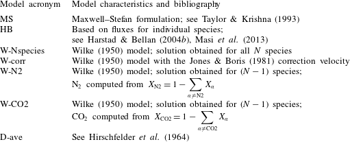
Models used to perform calculations to reproduce the Duncan & Toor (Reference Duncan and Toor1962) experiments.

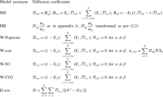
Seven different diffusion models are listed in tables 1 and 2, and calculations performed with them are compared with the two DT experiments. The first model is that of Maxwell and Stefan (MS in tables 1 and 2; see Taylor & Krishna Reference Taylor and Krishna1993), in which the binary-diffusion coefficients are used to compute the gradients of the chemical potentials of species
 $\unicode[STIX]{x1D6FC}$
,
 $\unicode[STIX]{x1D707}_{\unicode[STIX]{x1D6FC}}$
,
 $$\begin{eqnarray}\frac{\unicode[STIX]{x1D735}\unicode[STIX]{x1D707}_{\unicode[STIX]{x1D6FC}}}{R_{u}T}=\mathop{\sum }_{\unicode[STIX]{x1D6FC}=1,\unicode[STIX]{x1D6FC}\neq \unicode[STIX]{x1D6FD}}^{N}\frac{X_{\unicode[STIX]{x1D6FC}}X_{\unicode[STIX]{x1D6FD}}}{n{\mathcal{D}}_{\unicode[STIX]{x1D6FC}\unicode[STIX]{x1D6FD}}}\left(\frac{\boldsymbol{j}_{\unicode[STIX]{x1D6FC}}}{X_{\unicode[STIX]{x1D6FC}}}-\frac{\boldsymbol{j}_{\unicode[STIX]{x1D6FD}}}{X_{\unicode[STIX]{x1D6FD}}}\right),\end{eqnarray}$$
where
 $R_{u}$
is the universal gas constant and
 ${\mathcal{D}}_{\unicode[STIX]{x1D6FC}\unicode[STIX]{x1D6FD}}$
is the matrix of binary-diffusion coefficients. Except for binary mixtures for which Fick’s law is valid, the
 ${\mathcal{D}}_{\unicode[STIX]{x1D6FC}\unicode[STIX]{x1D6FD}}$
elements do not correspond to the species diffusion coefficients. The Harstad & Bellan (Reference Harstad and Bellan2004b
) formulation (HB in tables 1 and 2) performs a species-flux inversion of the MS matrix so that the diffusion coefficients are those appearing in the diffusion flux of each species (see appendix A). The Wilke (Reference Wilke1950) (W-Nspecies in tables 1 and 2) model relies on a diagonal diffusion matrix, and a solution is obtained for each of the
 $N$
species. The Wilke (Reference Wilke1950) model has been used in the past in conjunction with a correction velocity (Jones & Boris Reference Jones and Boris1981; Ern & Giovangigli Reference Ern and Giovangigli1999; Poinsot & Veynante Reference Poinsot and Veynantes2005) (W-corr in tables 1 and 2) to impose the physical constraint
 $\sum _{\unicode[STIX]{x1D6FC}=1}^{N}\boldsymbol{j}_{\unicode[STIX]{x1D6FC}}=0$
, which enforces mass conservation. It is also conceivable to obtain a solution for only (
 $N-1$
) species using the Wilke (Reference Wilke1950) model and utilizing the conservation of mass relationship
 $\sum _{\unicode[STIX]{x1D6FC}=1}^{N}X_{\unicode[STIX]{x1D6FC}}=1$
to obtain the
 $N$
th species molar fraction. Two such models are used here, denoted W-N2 and W-CO2 in tables 1 and 2, where the highlighted species is obtained from the conservation of mass mathematical statement. Finally, the simplest diffusion model is that of a diagonal diffusion matrix with constant coefficients (an example of this model is that using the unity Lewis number assumption, which is very popular in combustion mathematical formulations; see Poinsot & Veynante Reference Poinsot and Veynantes2005); this model is labelled D-ave in tables 1 and 2, and the correction velocity based on it is null.
Diffusion coefficients in the models used to perform calculations to reproduce the Duncan & Toor (Reference Duncan and Toor1962) experiments. For the MS formulation, the coefficients are listed for an ideal-gas mixture.

Initial conditions of two of the Duncan & Toor (Reference Duncan and Toor1962) experiments.

2.1.2 Evaluation of several diffusion models
The DT experiments consist of ternary species mixing for which the MS solution is still computationally tractable in an efficient manner. For notation purposes, each species is here associated with a number: nitrogen (1), hydrogen (2) and carbon dioxide (3); the corresponding values of the binary-diffusion coefficients for
 $T=308.3~\text{K}$
and at
 $p=1$
atm are
 ${\mathcal{D}}_{12}=8.33\times 10^{-5}~\text{m}^{2}~\text{s}^{-1}$
,
 ${\mathcal{D}}_{13}=1.68\times 10^{-5}~\text{m}^{2}~\text{s}^{-1}$
and
 ${\mathcal{D}}_{23}=6.8\times 10^{-5}~\text{m}^{2}~\text{s}^{-1}$
. The initial conditions in each experiment are listed in table 3. Bulb A is represented in the simulations by the linear domain [
 $0,0.5$
] and bulb B by the domain [
 $0.5,1$
]. For numerical reasons, the initial condition is prescribed as a hyperbolic tangent of width 0.01 between the [
 $0,0.5$
] and [
 $0.5,1$
] regions of the domain. The [
 $0,1$
] domain is discretized with
 $201$
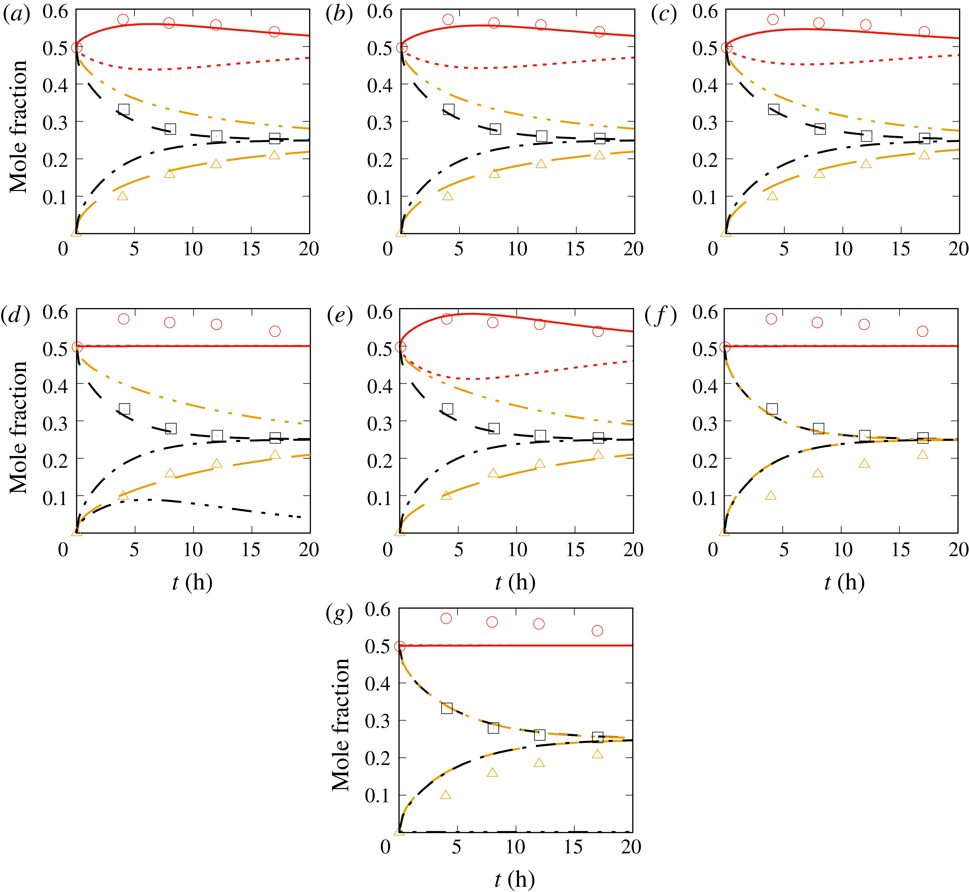
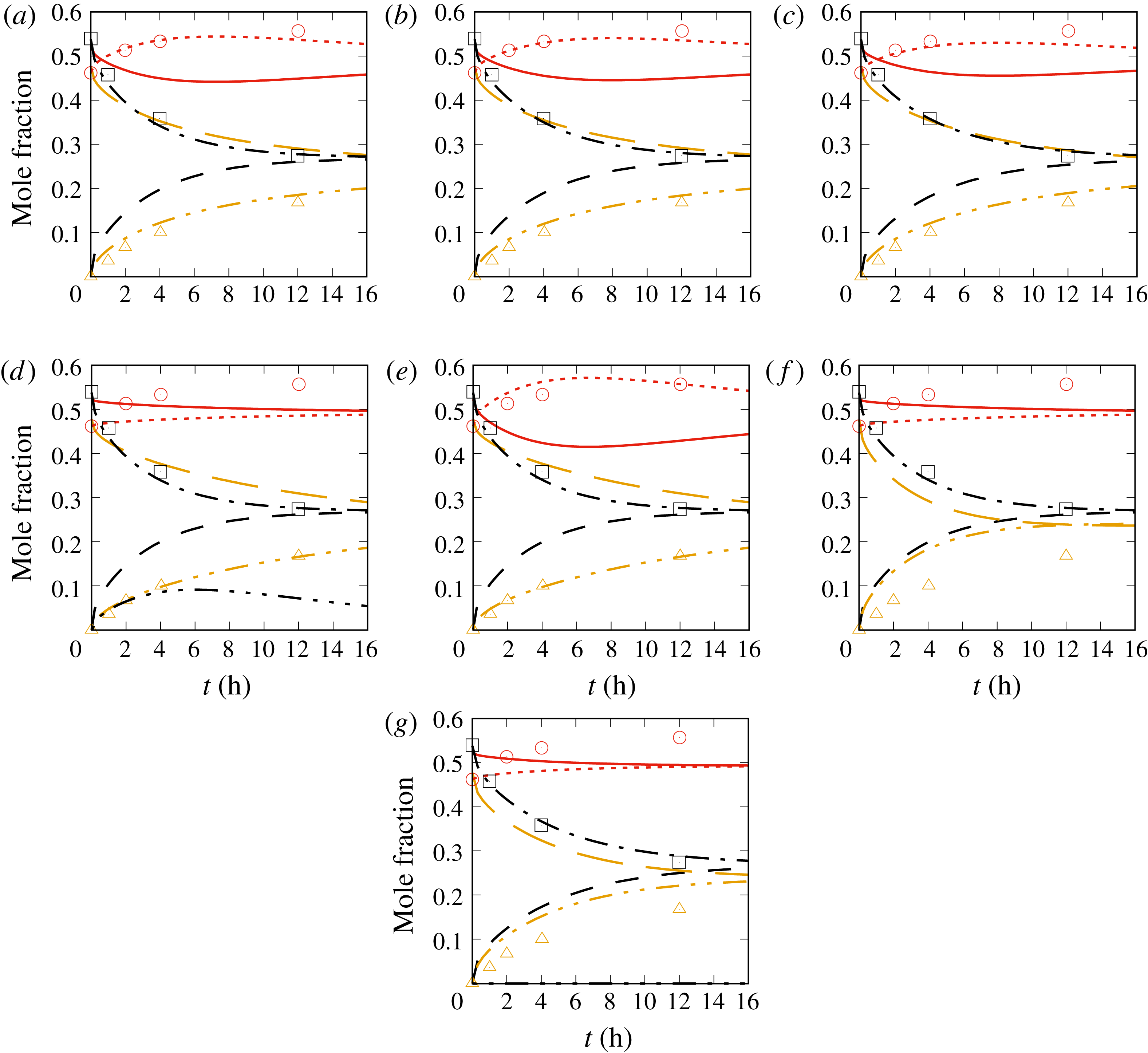
points. Both time and spatial convergence have been investigated by doubling the spatial and temporal resolution, with no effect on the results. Figure 1 illustrates the results of DT1 and figure 2 depicts the results of DT2. All mole fraction quantities represent spatial integrals over the corresponding regions of the domain, e.g.
 $$\begin{eqnarray}X_{\text{N2}}^{A}(t)=\frac{1}{0.5}\int _{0}^{0.5}X_{\text{N2}}(x,t)\,\text{d}x\quad \text{and}\quad X_{\text{N2}}^{B}(t)=\frac{1}{0.5}\int _{0.5}^{1}X_{\text{N2}}(x,t)\,\text{d}x.\end{eqnarray}$$
One-dimensional simulations to reproduce the DT1 experiment that are performed with different diffusion matrices. The model acronyms are listed in table 1: (a) MS, (b) HB, (c) W-corr, (d) W-Nspecies, (e) W-N2, (f) W-CO2, (g) D-ave. The symbols are the experimental results for bulb A. The legend is as follows: - - - -,
 $X_{\text{N2}}^{A};$
– – –,
 $X_{\text{H2}}^{A};$
— ⋅ ⋅ —,
 $X_{\text{CO2}}^{A};$
——,
 $X_{\text{N2}}^{B}$
; — ⋅ —,
 $X_{\text{H2}}^{B};$
— —,
 $X_{\text{CO2}}^{B}$
, where the superscripts refer to the bulb. The curves identified by –
 $\cdots \,$
– show the departure from mass conservation.

One-dimensional simulations to reproduce the DT2 experiment that are performed with different diffusion matrices. The model acronyms are listed in table 1: (a) MS, (b) HB, (c) W-corr, (d) W-Nspecies, (e) W-N2, (f) W-CO2, (g) D-ave. The symbols are the experimental results for bulb A. The legend is as follows: - - - -,
 $X_{\text{N2}}^{A};$
– – –,
 $X_{\text{H2}}^{A}$
; — ⋅ ⋅ —,
 $X_{\text{CO2}}^{A};$
——,
 $X_{\text{N2}}^{B};$
— ⋅ —,
 $X_{\text{H2}}^{B};$
— —,
 $X_{\text{CO2}}^{B}$
, where the superscripts refer to the bulb. The curves identified by –
 $\cdots \,$
– show the departure from mass conservation.

The results of figures 1 and 2 show the same trends. Both the MS and HB models reproduce well the DT1 and DT2 experiments, in particular the uphill diffusion of
 $\text{N}_{2}$
, and its time evolution to an eventual equilibrium to be reached past the experimental times of 20 h and 16 h respectively. The W-corr model captures the
 $\text{N}_{2}$
uphill diffusion and the other species behaviour; however, it underestimates uphill diffusion and appears to be less accurate than either the MS or the HB model. For the DT1 experiment, the inaccuracies are manifested in the W-corr model results at early time, while in the DT2 experiment, the lack of high fidelity is clear at later times; the erratic timewise comparison with experiment signifies that the model is not timewise reliable. The W-Nspecies model does not conserve mass and it is also unable to reproduce uphill diffusion. However, when the same diffusion model is used with only
 $X_{\text{H2}}$
and
 $X_{\text{CO2}}$
as evolution variables, and
 $X_{\text{N2}}$
is computed by enforcing mass conservation – model W-N2 – the results do capture the
 $\text{N}_{2}$
uphill diffusion although they overpredict it with respect to the MS and HB models. Additionally, when the same diffusion model is used with
 $X_{\text{H2}}$
and
 $X_{\text{N2}}$
as evolution variables, and mass conservation is enforced by computing
 $X_{\text{CO2}}$
instead of
 $X_{\text{N2}}$
, the results no longer capture
 $\text{N}_{2}$
uphill diffusion. It is thus concluded that the class of W diffusion models (W-Nspecies, W-N2, W-CO2) is unreliable as a predictive tool. Finally, the D-ave model conserves mass, but cannot reproduce uphill diffusion, in that the model predicts
 $\text{N}_{2}$
to be in equilibrium or close to equilibrium between the two bulbs during the observation time.
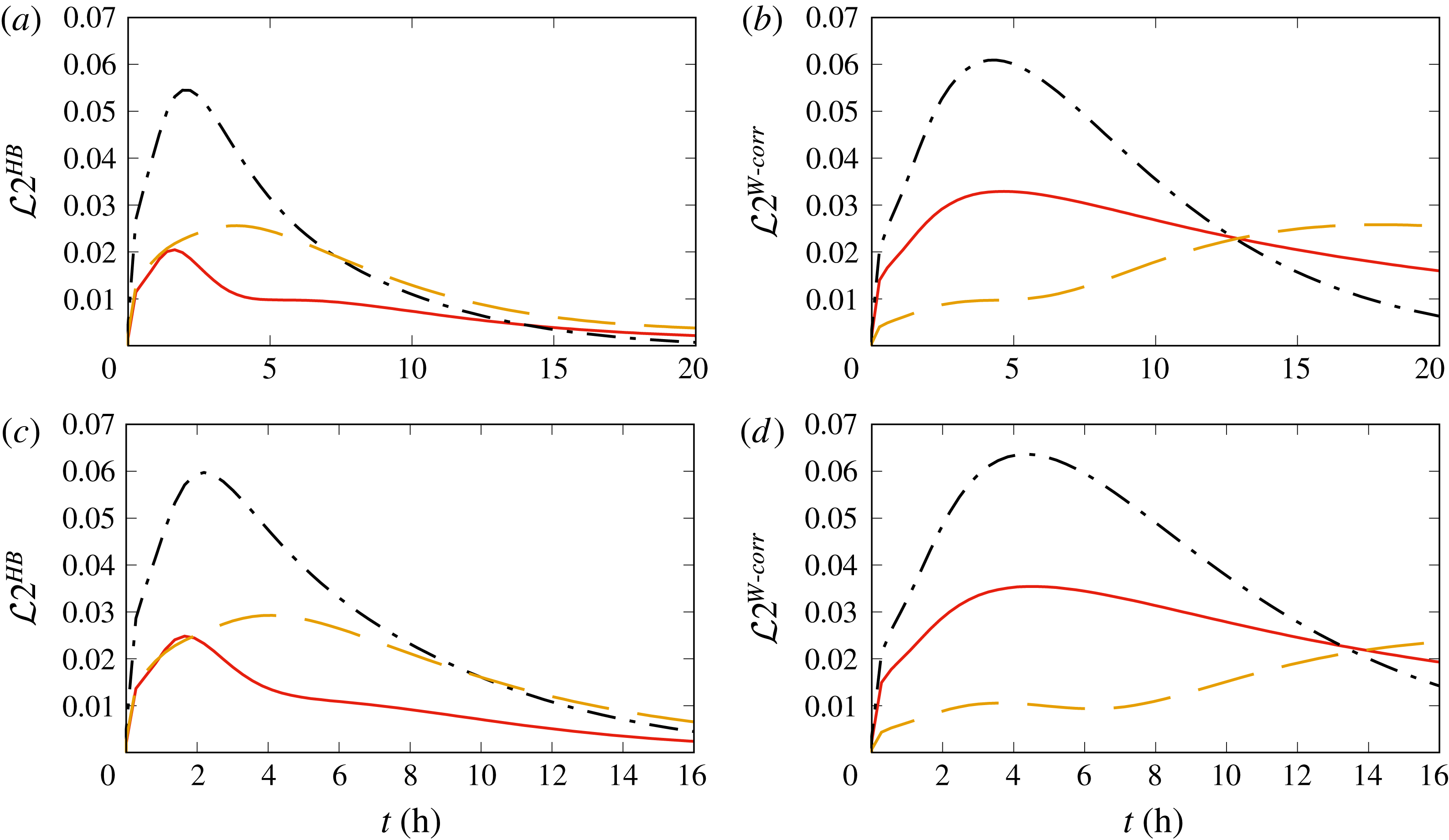
The timewise evolution of the
 ${\mathcal{L}}2_{\unicode[STIX]{x1D6FC}}^{{\mathcal{M}}}$
norm, computing relative errors between (a,c) the HB model solution and the MS solution of the DT experiments and (b,d) the W-corr model solution and the MS solution of the DT experiments, for (a,b) the DT1 experiment and (c,d) the DT2 experiment. For all panels: ——,
 $X_{\text{N2}}$
; — ⋅ —,
 $X_{\text{H2}}$
; — —,
 $X_{\text{CO2}}$
.

Considering the MS model as the template against which other models can be assessed, it is instructive to now focus on the spatial distribution of the compositional fields. To quantitatively determine the performance of the models in predicting uphill diffusion, the relative error is computed using the
 ${\mathcal{L}}2$
norm in order to evaluate the departure of the HB and W-corr models from the MS model, and the results are presented in figure 3 for both the DT1 and DT2 experiments. The relative error is computed from the numerical solution obtained with a discretization of
 ${\mathcal{N}}$
points as
 $$\begin{eqnarray}{\mathcal{L}}2_{\text{N2}}^{{\mathcal{M}}}(t)=\frac{\sqrt{\displaystyle \mathop{\sum }_{i=1}^{{\mathcal{N}}}[X_{\text{N2}}^{{\mathcal{M}}}(x_{i},t)-X_{\text{N2}}^{MS}(x_{i},t)]^{2}}}{\sqrt{\displaystyle \mathop{\sum }_{i=1}^{{\mathcal{N}}}X_{\text{N2}}^{MS}(x_{i},t)^{2}}}\end{eqnarray}$$
as an example for
 $X_{\text{N2}}$
, where the superscript MS denotes the model listed in table 1 and
 ${\mathcal{M}}$
labels either HB or W-corr; thus, the results do not measure the differences seen in figures 1 and 2 which pertain to temporal variation of spatial averages according to (2.6). The relative error is computed at intervals of
 $0.274$
hours. The illustrations of figure 3 show that although the model errors are somewhat larger for the DT2 experiment compared with the DT1 experiment, the trends are similar for a specific
 ${\mathcal{M}}$
. The first observation is that the maximum
 ${\mathcal{L}}2_{\unicode[STIX]{x1D6FC}}^{{\mathcal{M}}}(t)$
is similar for HB and W-corr, although slightly smaller for the HB model. For the HB model, the largest errors (
 $\simeq 5.5\,\%$
for DT1 and
 $\simeq 5.8\,\%$
for DT2) occur approximately 2–3 h from the calculation initiation, and the largest error is for
 $X_{\text{H2}}$
while the smallest error is for
 $X_{\text{N2}},$
i.e. the uphill-diffusing species. After the 2–3 h stage, the errors decline monotonically very rapidly, and by 10 h they are negligible (i.e.
 $O(10^{-1})\%$
), so that it is clear that they will be close to null well before the time when experimental equilibrium occurs. The situation is entirely different for the W-corr model. First, the maximum error (
 $\simeq 6.0\,\%$
for DT1 and
 $\simeq 6.3\,\%$
for DT2) occurs for
 $X_{\text{H2}}$
approximately 4–5 h after the start of the experiment and the smallest error is initially incurred by
 $X_{\text{CO2}}$
; past 4–5 h, the errors on
 $X_{\text{H2}}$
and
 $X_{\text{N2}}$
decay monotonically very slowly, particularly for
 $X_{\text{N2}}$
, so that by the end time of the documented data, these errors have not abetted substantially. Even more worrisome is the fact that the error in
 $X_{\text{CO2}}$
, after reaching a plateau, monotonically increases with
 $t$
, so that by the end of the documented experimental data, it has become the largest error. Thus, during the time of the experimentally documented data, the error between the HB and MS predictions decreases considerably to negligible values, whereas the error between the W-corr and MS predictions increases considerably. Moreover, most likely, the W-corr calculation would not have reached the equilibrium state by the time that the experiment shows equilibrium; that is, the W-corr simulation does not converge to equilibrium at the correct time rate. Thus, any process in which transient calculations are important will not be well represented by the W-corr model.
2.1.3 Conclusions from evaluation of existing diffusion models
Some, but not all, of the comparisons of figures 1 and 2 appear in Taylor & Krishna (Reference Taylor and Krishna1993), and the authors are not aware of published evaluations similar to those of figure 3. Considering the goals of this study, comparison of all existing diffusion models with the same data allows definitive conclusions on the suitability of these models for identification of thermodynamic regimes. The first conclusion is that the MS model, which is computationally intensive to use for multispecies flows, provides in the computationally efficient three-species DT experiments situation a quantitatively accurate half-domain-average composition when compared with the DT1 and DT2 experiments. None of the models based on the Wilke (Reference Wilke1950) approximation can reliably reproduce the half-domain-average composition as a function of time. When the Wilke (Reference Wilke1950) model is used with a velocity correction, an approximately accurate half-domain-average composition is obtained, but consideration of the detailed compositional field shows that the detailed field timewise evolution is different from that of the template MS model, and thus neither the timewise evolution nor the time necessary to converge to equilibrium is well reproduced compared with the template; thus, the seemingly favourable comparison obtained in figures 1 and 2 is deceptive for evaluating the potential of this model for detailed simulations. We attribute the inability of the W-corr model to reproduce the spatiotemporal variation of the template to the fact that the model ignores the important effects of the diffusion among species, i.e. the off-diagonal elements of the diffusion matrix, and only considers the diffusional interaction of each species with the global mixture represented by the ensemble of other species. Thus, it is not advisable to use this model for computing thermodynamic regimes because these are strong functions of the compositional field. The second conclusion is that the Harstad & Bellan (Reference Harstad and Bellan2004b
) model used in Masi et al. (Reference Masi, Bellan, Harstad and Okong’o2013) and Bellan (Reference Bellan2017) is quantitatively accurate (for conditions for which data are available) in that initial errors, as examined through the
 ${\mathcal{L}}2$
norm, decay very rapidly; thus, the model has the correct timewise behaviour in that it converges to the equilibrium state at the same rate as the MS template. No equivalent high-
 $p$
experimental data (to the DT data) exist for evaluating the Harstad & Bellan (Reference Harstad and Bellan2004b
) model under those conditions. Since the Masi et al. (Reference Masi, Bellan, Harstad and Okong’o2013) and Bellan (Reference Bellan2017) databases are the only high-
 $p$
DNS databases obtained with the Harstad & Bellan (Reference Harstad and Bellan2004b
) model, they can be considered as those most likely to be able to provide quantitatively accurate information for computing the thermodynamic regime of such mixtures under these (
 $p,T$
) conditions.
2.2 Spinodal locus computation
The spinodal locus is a hypersurface in the thermodynamic phase space that separates the stable thermodynamic regime in which equilibrium among phases holds from the unstable thermodynamic regime in which phases are no longer in equilibrium (Taylor & Krishna Reference Taylor and Krishna1993); in the unstable regime, spinodal decomposition occurs (Debenedetti Reference Debenedetti1996; Tester & Modell Reference Tester and Modell1997; Abu-Eishah, Darwish & Aljundi Reference Abu-Eishah, Darwish and Aljundi1998; Stradi et al. Reference Stradi, Brennecke, Kohn and Stadtherr2001; Nichita & Gomez Reference Nichita and Gomez2010) that may be initiated by uphill diffusion. Between the stable and unstable regimes are the metastable-liquid bubble regime and the metastable-vapour nucleation regime. In the thermodynamically stable regime, the thermodynamic information suffices to describe a system. Any transient situation, for example an unsteady evaporating spray, is thermodynamically located in the unstable or the metastable region of the thermodynamic phase space; that is, additional to the thermodynamic information, time-dependent conservation equations are required to describe the system. The metastable regions of the thermodynamic phase diagram could host such sprays as long as the characteristic time of the life span of the spray is much larger than the characteristic time of the metastable state.
For single species, the instability is simultaneously of mechanical and thermal type; the necessary and sufficient condition for stability is that the isobaric heat capacity (thermal) or the isothermal compressibility (mechanical) be positive. These two criteria are equivalent and, if violated, the violation is simultaneous (Debenedetti Reference Debenedetti1996). For example, near the critical point of a single species, the density can have unbounded fluctuations. Unlike for single species, multispecies mixtures may have composition fluctuations (Debenedetti Reference Debenedetti1996; Tester & Modell Reference Tester and Modell1997), and thus the instability is in this case of compositional nature rather than of mechanical origin. This type of instability is called ‘diffusional’ or ‘material’ instability, and can lead to either phase or species segregation. The stability condition for a multispecies mixture is (Debenedetti Reference Debenedetti1996; Tester & Modell Reference Tester and Modell1997)
 $$\begin{eqnarray}-\!\left(\frac{\unicode[STIX]{x2202}\unicode[STIX]{x1D707}_{\unicode[STIX]{x1D6FC}}}{\unicode[STIX]{x2202}n_{\unicode[STIX]{x1D6FC}}}\right)_{T,P,n_{\unicode[STIX]{x1D6FD}}(\unicode[STIX]{x1D6FC}\neq \unicode[STIX]{x1D6FD})}>0,\end{eqnarray}$$
where
 $n_{\unicode[STIX]{x1D6FC}}=nX_{\unicode[STIX]{x1D6FC}}$
is the number of moles of species
 $\unicode[STIX]{x1D6FC}$
. Whenever (2.8) is violated, a multispecies system undergoes phase separation.
To clarify the relationship between phase separation and spinodal decomposition, we recall the following definitions: the spinodal locus is the boundary between the unstable and stable (or metastable) regimes; a single phase is a region characterized by microscopic (and macroscopic) homogeneity at the continuum scale; the metastable regime is a single phase that lacks microscopic homogeneity or equivalently has rough macroscopic homogeneity (Debenedetti Reference Debenedetti1996). Phase separation can refer to either fluid–gas or fluid–fluid separation. To distinguish between these two types of separation, we shall refer to fluid–gas separation as phase separation (i.e. one phase becoming two phases) and fluid–fluid separation as species segregation (i.e. in a species mixture, one of the species separates from the others, with the result that regions of the spatial domain are solely occupied by that species). Phase separation may occur through uphill diffusion. Uphill diffusion, which can occur over the entire thermodynamic phase space (e.g. see Krishna (Reference Krishna2015)), leads to enhanced density gradients which affect turbulence and vorticity production in a flow (Hannoun, Fernando & List Reference Hannoun, Fernando and List1988; Masi et al. Reference Masi, Bellan, Harstad and Okong’o2013), showing the strong coupling between thermodynamics and dynamics in this regime. On the other hand, in phase separation (i.e. spinodal decomposition), uphill diffusion may or may not play a role; for example, phase separation may be achieved by simply reducing the temperature.
Clearly, it is important to identify the thermodynamically unstable regions of a compositionally complex mixture through computations of the spinodal, and to determine whether spinodal decomposition occurs in a flow. To this end, we wish to demonstrate an accurate and reliable methodology for computing the spinodal of multispecies mixtures. Here, we select to compare our computations with binary, ternary and quaternary mixtures for which data exist in the literature.
Computation of the stability condition from (2.8) for a pressure-explicit EOS is costly as it involves the calculation of the first and second derivative with respect to the number of moles and the derivative with respect to volume,
 $V$
. Another method, computationally less expensive, has been proposed in the past by Heidemann & Khalil (Reference Heidemann and Khalil1980): a criterion for the critical locus is found by examining the stability of homogeneous phases. A given phase held at a specific condition will be stable if for every isothermal variation
 $$\begin{eqnarray}\left[A-A_{0}+p_{0}(V-V_{0})-\mathop{\sum }_{\unicode[STIX]{x1D6FC}}\unicode[STIX]{x1D707}_{\unicode[STIX]{x1D6FC}0}(n_{\unicode[STIX]{x1D6FC}}-n_{\unicode[STIX]{x1D6FC}0})\right]>0,\end{eqnarray}$$
where
 $A$
is the Helmholtz free energy and the subscript
 $0$
denotes the test condition of interest. A change in
 $V$
or
 $n$
does not qualify as a change of phase, and, to discard this possibility,
 $(V-V_{0})$
is set to be null, so that the criterion becomes
 $$\begin{eqnarray}\left[A-A_{0}-\mathop{\sum }_{\unicode[STIX]{x1D6FC}}\unicode[STIX]{x1D707}_{\unicode[STIX]{x1D6FC}0}(n_{\unicode[STIX]{x1D6FC}}-n_{\unicode[STIX]{x1D6FC}0})\right]>0.\end{eqnarray}$$
The Helmholtz free energy can be expanded in a Taylor series around the test condition,
 $$\begin{eqnarray}\displaystyle & & \displaystyle \left[A-A_{0}-\mathop{\sum }_{\unicode[STIX]{x1D6FC}}\unicode[STIX]{x1D707}_{\unicode[STIX]{x1D6FC}0}\unicode[STIX]{x0394}n_{\unicode[STIX]{x1D6FC}}\right]=\frac{1}{2!}\mathop{\sum }_{\unicode[STIX]{x1D6FD}}\mathop{\sum }_{\unicode[STIX]{x1D6FC}}\left(\frac{\unicode[STIX]{x2202}^{2}A}{\unicode[STIX]{x2202}n_{\unicode[STIX]{x1D6FD}}\unicode[STIX]{x2202}n_{\unicode[STIX]{x1D6FC}}}\right)\unicode[STIX]{x0394}n_{\unicode[STIX]{x1D6FC}}\unicode[STIX]{x0394}n_{\unicode[STIX]{x1D6FD}}\nonumber\\ \displaystyle & & \displaystyle \quad +\,\frac{1}{3!}\mathop{\sum }_{\unicode[STIX]{x1D6FE}}\mathop{\sum }_{\unicode[STIX]{x1D6FD}}\mathop{\sum }_{\unicode[STIX]{x1D6FC}}\left(\frac{\unicode[STIX]{x2202}^{3}A}{\unicode[STIX]{x2202}n_{k}\unicode[STIX]{x2202}n_{j}\unicode[STIX]{x2202}n_{i}}\right)\unicode[STIX]{x0394}n_{\unicode[STIX]{x1D6FC}}\unicode[STIX]{x0394}n_{\unicode[STIX]{x1D6FD}}\unicode[STIX]{x0394}n_{k\unicode[STIX]{x1D6FE}}+O(\unicode[STIX]{x0394}n^{4}),\end{eqnarray}$$
where
 $\unicode[STIX]{x1D6E5}$
indicates a variation. Stability is assured if the quadratic term in (2.11) is positive definite. A necessary condition for a point to lie on the limit of stability is that the Hessian,
 $\boldsymbol{Q}$
, of the Helmholtz free energy,
 $$\begin{eqnarray}Q_{\unicode[STIX]{x1D6FC}\unicode[STIX]{x1D6FD}}=\frac{\unicode[STIX]{x2202}^{2}A}{\unicode[STIX]{x2202}n_{\unicode[STIX]{x1D6FD}}\unicode[STIX]{x2202}n_{\unicode[STIX]{x1D6FC}}},\end{eqnarray}$$
should have a null determinant. The stability condition is therefore given by the condition
 $$\begin{eqnarray}\det \boldsymbol{Q}>0,\end{eqnarray}$$
where
 $$\begin{eqnarray}Q_{\unicode[STIX]{x1D6FC}\unicode[STIX]{x1D6FD}}=\left(\frac{\unicode[STIX]{x2202}^{2}A}{\unicode[STIX]{x2202}n_{\unicode[STIX]{x1D6FC}}\unicode[STIX]{x2202}n_{\unicode[STIX]{x1D6FD}}}\right)_{T,V}=R_{u}T\left(\frac{\unicode[STIX]{x2202}\log f_{\unicode[STIX]{x1D6FC}}}{\unicode[STIX]{x2202}n_{\unicode[STIX]{x1D6FD}}}\right)_{T,V};\end{eqnarray}$$
here,
 $f_{\unicode[STIX]{x1D6FC}}$
is the fugacity. Details about the Peng–Robinson (PR) EOS and the computation of the relative fugacity function are given in appendix C. Other methods are available to compute the spinodal locus (Debenedetti Reference Debenedetti1996; Poling, Prausnitz & O’Connell Reference Poling, Prausnitz and O’Connell2001); however, the method of Heidemann & Khalil (Reference Heidemann and Khalil1980) is preferred due to the well-known properties of robustness and computational speed (Heidemann & Khalil Reference Heidemann and Khalil1980; Abu-Eishah et al.
Reference Abu-Eishah, Darwish and Aljundi1998; Poling et al.
Reference Poling, Prausnitz and O’Connell2001; Nichita & Gomez Reference Nichita and Gomez2010). To perform the computation,
 $v$
and the composition
 $\{X_{\unicode[STIX]{x1D6FC}}\}$
, where
 $\unicode[STIX]{x1D6FC}\in [1,N]$
, are selected, and the value of
 $T$
is computed from
 $\det \boldsymbol{Q}=0$
; then,
 $p$
is computed from the EOS. The computation is initialized with a guessed value of
 $T$
and proceeds iteratively. The numerical implementation uses a bounded Newton–Raphson method (Press et al.
Reference Press, Teukolsky, Vetterling and Flannery1992) and employs the difference in
 $T$
between iterations to check convergence. In general, because at fixed composition the dimensionality of the spinodal locus is
 $1$
– a line
 $f(T(v))$
– it is also useful to visualize it as a function of
 $X_{\unicode[STIX]{x1D6FC}};$
if
 $v$
is also fixed, the locus is a single point.
To test the implementation of the Heidemann & Khalil (Reference Heidemann and Khalil1980) method, single-species, binary, ternary and quaternary species mixture spinodal loci are computed and the results are compared with experimental data or other existing accepted information; these computations are presented in appendix D. These locus computations and the agreement with available data demonstrate that the adopted spinodal computation methodology is reliable and accurate. Henceforth, we adopt the terminology of ‘below’ the spinodal to refer to the unstable region and ‘above’ the spinodal to be the complementary of the ‘above the spinodal’ in the phase space. In the
 $(p,T)$
plane, the region of thermodynamic instability is always to the right of the stability limit curve when moving in the direction of increasing molar volume (Heidemann & Khalil Reference Heidemann and Khalil1980).
3 Thermodynamic regimes for high-
 $p$
turbulent multispecies mixing and reacting flows

3.1 Peculiarities of the spinodal locus for a multispecies mixture
Thermodynamic considerations using a cubic EOS in the variable
 $v$
(e.g. the PR EOS) for a single species show that at specified
 $(p,T),$
 $v$
is not uniquely defined. This lack of uniqueness is due to the fact that the EOS has either a real
 $v$
root and two non-physical imaginary roots, in which case it corresponds to a single phase, or three real roots, with the smallest root,
 $v_{l}$
, associated with the liquid phase (as long as the root is larger than the co-volume Lawal (Reference Lawal.1987)), the largest root,
 $v_{v}$
, associated with the vapour phase and the middle root considered to be unstable and discarded (it lies below the spinodal). It is possible that two of the real roots may also coincide, in which case this condition is identified as a critical state. These considerations indicate that the EOS is not sufficient to indicate whether a system is in the liquid or gas phase; the Navier–Stokes conservation equations are necessary to make this identification (De Groot & Mazur Reference De Groot and Mazur1984). Since for a single-species situation the composition is known, the solution of the conservation equations provides
 $(\unicode[STIX]{x1D70C},e_{t},\boldsymbol{u})$
, where
 $e_{t}=e+(u_{i}u_{i})/2$
is the total specific energy and
 $e$
is the specific internal energy; thus, when using
 $(\unicode[STIX]{x1D70C},e)$
in conjunction with the EOS, one may solve for
 $(p,T).$
At any given spatial location, using these values of
 $(p,T)$
in the EOS, one may solve for
 $v.$
As already stated, there may be several
 $v$
roots, but only one of the roots will yield through
 $\unicode[STIX]{x1D70C}=mv^{-1}$
the
 $\unicode[STIX]{x1D70C}$
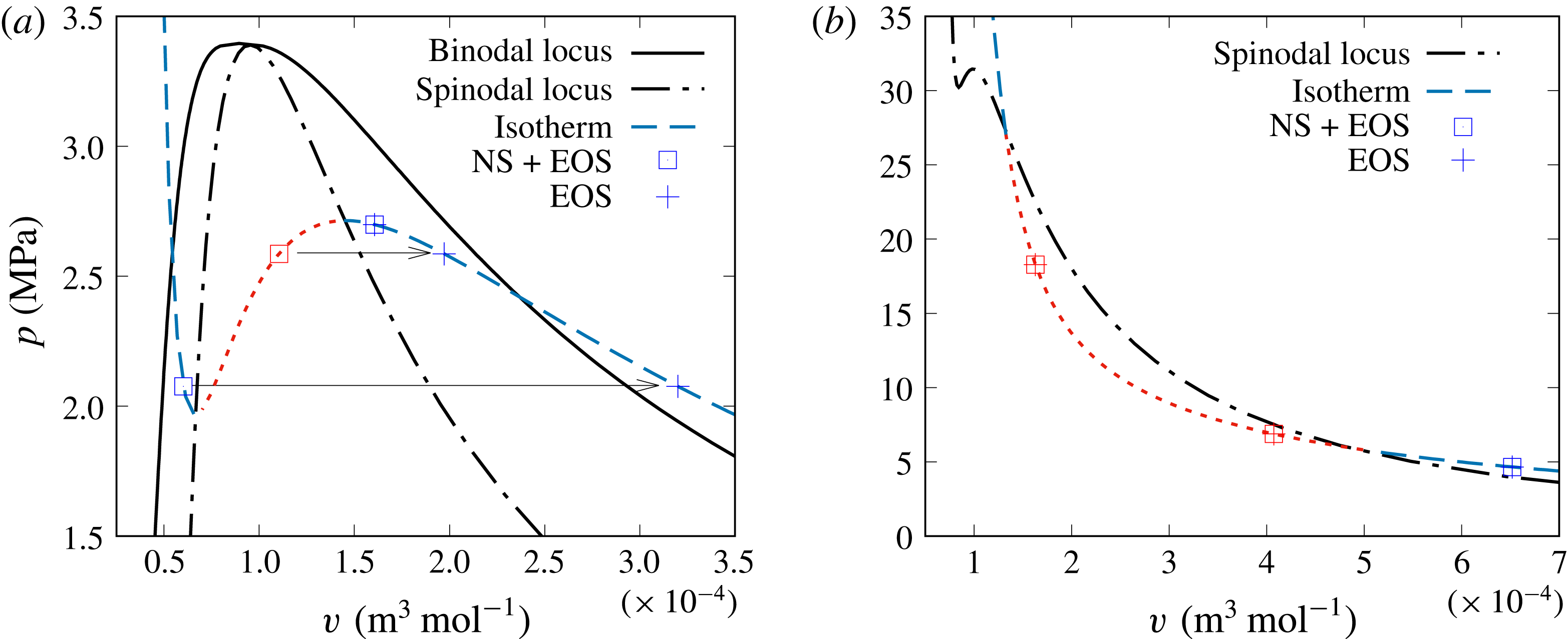
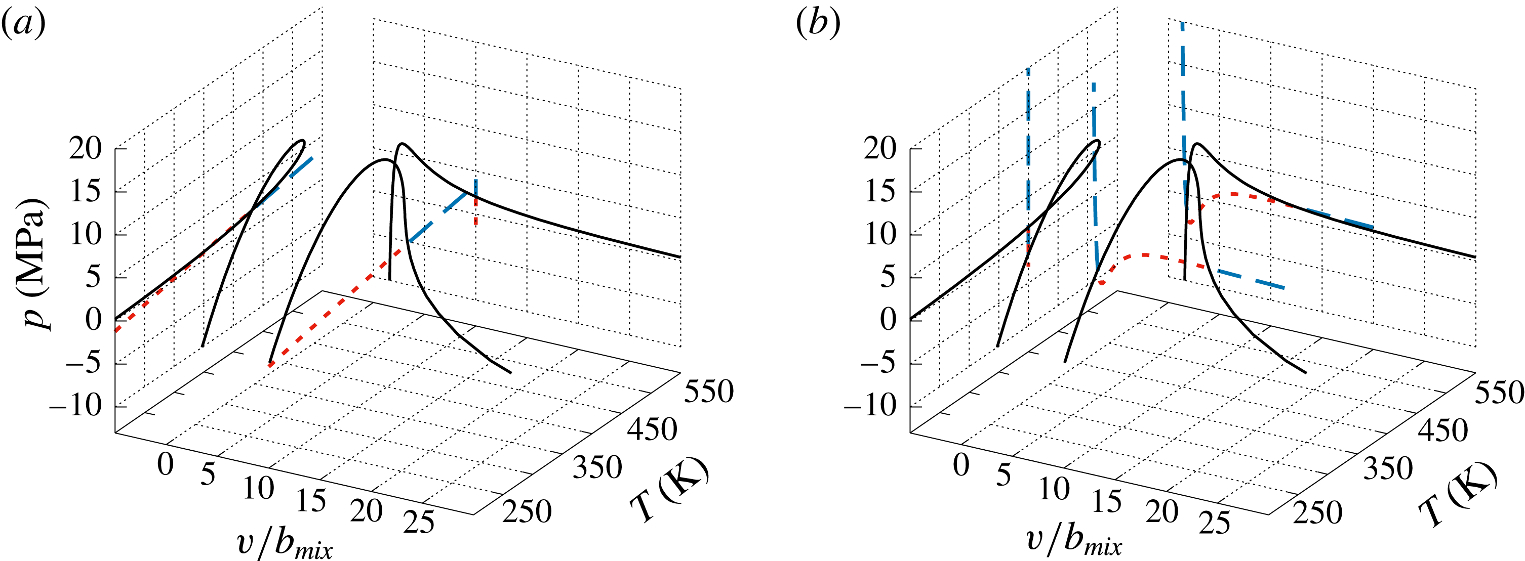
value computed from the solution of the conservation equations. Therefore, for a single species, it is straightforward to identify the phase of the mixture, as graphically shown in figure 4(a) for
 $\text{N}_{2}$
. The binodal in figure 4(a) is computed using the National Institute of Standards and Technology software Refprop (Lemmon, Huber & McLinden Reference Lemmon, Huber and McLinden2013), while all other information is calculated utilizing the PR EOS. Three points are selected to mimic
 $(p,T,v)$
states provided by the conservation equations in conjunction with the EOS: one point is in the metastable-liquid bubble regime, the second point is in the unstable regime and the third point is in the metastable-vapour nucleation regime. In this case, selecting
 $v_{v}$
corresponds to the value of
 $\unicode[STIX]{x1D70C}$
obtained from the conservation equations, and the state is in the metastable-vapour regime. Therefore, for a single species, matching
 $v_{v}$
obtained from solving the PR (or any cubic) EOS to
 $\unicode[STIX]{x1D70C}$
guarantees that the state will be in the vapour phase or supercritical regime, and, conversely, matching
 $v_{l}$
obtained from solving the PR (or any cubic) EOS to
 $\unicode[STIX]{x1D70C}$
guarantees that the state will be in the liquid phase regime. These straightforward considerations can be traced to the concave shape of the spinodal and to the shape of the isotherms, which have two inflection points, each of these points corresponding to an intersection with the spinodal. However, these geometrical consideration no longer hold for multispecies mixtures.
(a) Single species (
 $\text{N}_{2}$
) example of binodal and spinodal locus, and isotherm. Three
 $p$
points below the spinodal and on an isotherm show how the corresponding
 $v$
might not be unique. (b) Multispecies example of spinodal locus and isotherm. For the multispecies case, the selected
 $p$
on an isotherm corresponds to a unique
 $v$
.

Unlike for single species, for which the EOS has constant coefficients, the EOS for a multispecies mixture has coefficients which are functions of the thermodynamic variables. The result is that the simplicity of the binodal, spinodal and isothermal loci shapes, and of their relative positions, no longer holds. As a result, the spinodal may not have a simple geometrical interpretation in the
 $(p,v)$
plane, in particular because the spinodal locus is no longer the minimum or maximum on an isotherm as it is in the single-species case. In a multispecies mixture, it is possible that the projection on the
 $(p,v)$
plane of an isotherm may intersect the spinodal twice without inflections – i.e. the spinodal and isotherm loci can intersect several times in a region where
 $p$
is a monotonically decreasing function of
 $v$
– but in this region the EOS may only have one real
 $v$
root. For example, in figure 4(b), the spinodal locus computed for the five-species mixture of Masi et al. (Reference Masi, Bellan, Harstad and Okong’o2013) using the PR EOS is displayed along with an isotherm corresponding to
 $T=450~\text{K}$
which intersects the spinodal. Three fictitious solutions
 $(p,v,T,Y_{\unicode[STIX]{x1D6FC}})$
of the conservation equations coupled with the EOS are considered, all having the same composition
 $X_{\text{C7H16}}=0.4,X_{\text{N2}}=0.455$
,
 $X_{\text{O2}}=0.1,X_{\text{H2O}}=0.01$
and
 $X_{\text{CO2}}=0.035.$
For each of these states, for the corresponding
 $(p,T,Y_{\unicode[STIX]{x1D6FC}})$
, the EOS is solved for
 $v$
. It turns out that each of the three states exhibits a single
 $v$
real root, contrary to single-species results expectations (see figure 4
a) that the two states for which
 $p$
is smaller than the value of
 $p$
on the spinodal at the same
 $v$
should have multiple
 $v$
roots. Therefore, these two states are in the unstable regime, yet they exhibit a single real
 $v$
root. These considerations highlight the fact that for multispecies mixtures, the only option to determine the thermodynamic state is to compute the thermodynamic stability criterion represented by the spinodal instead of relying on the EOS roots as can be done for single species.
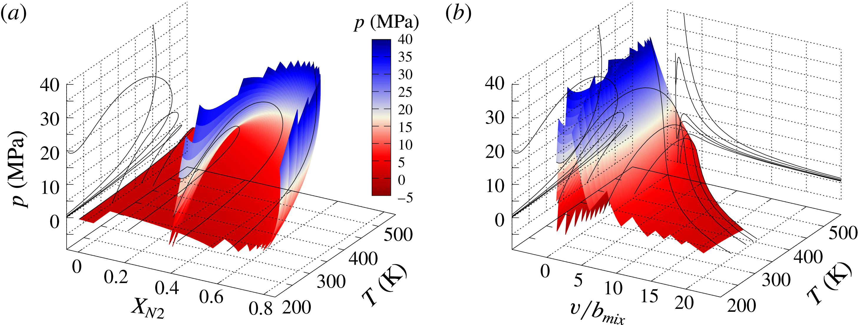
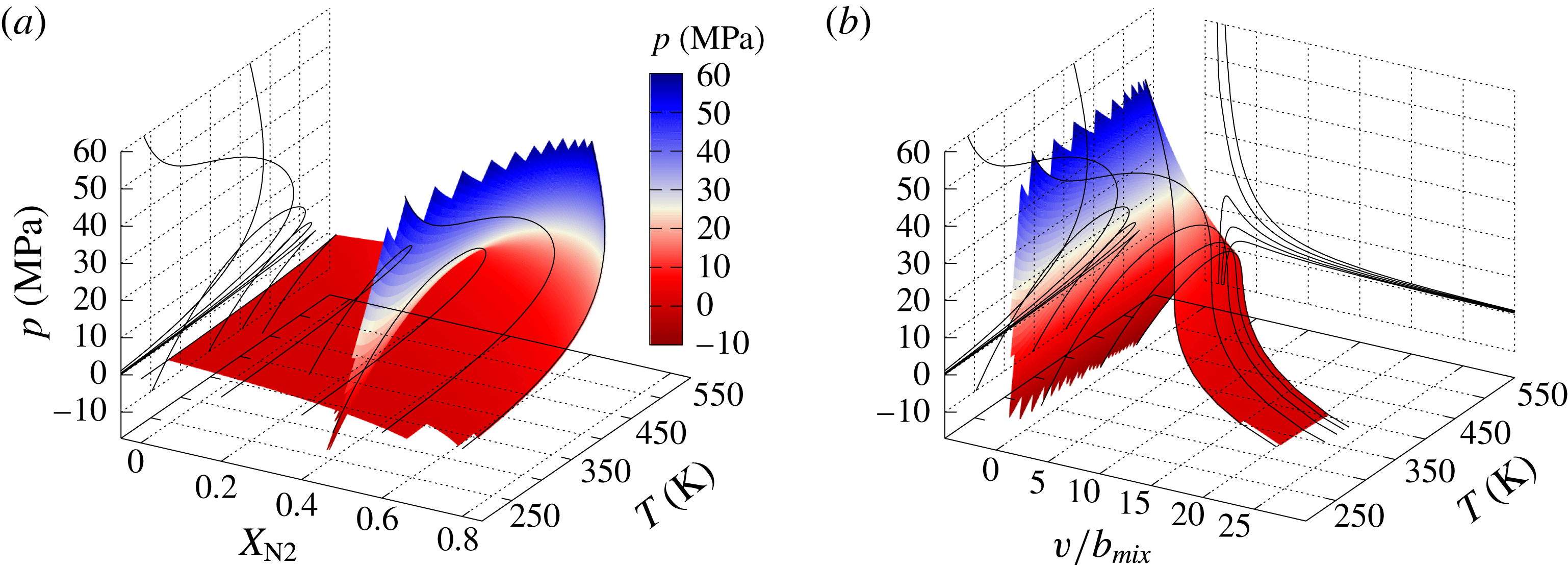
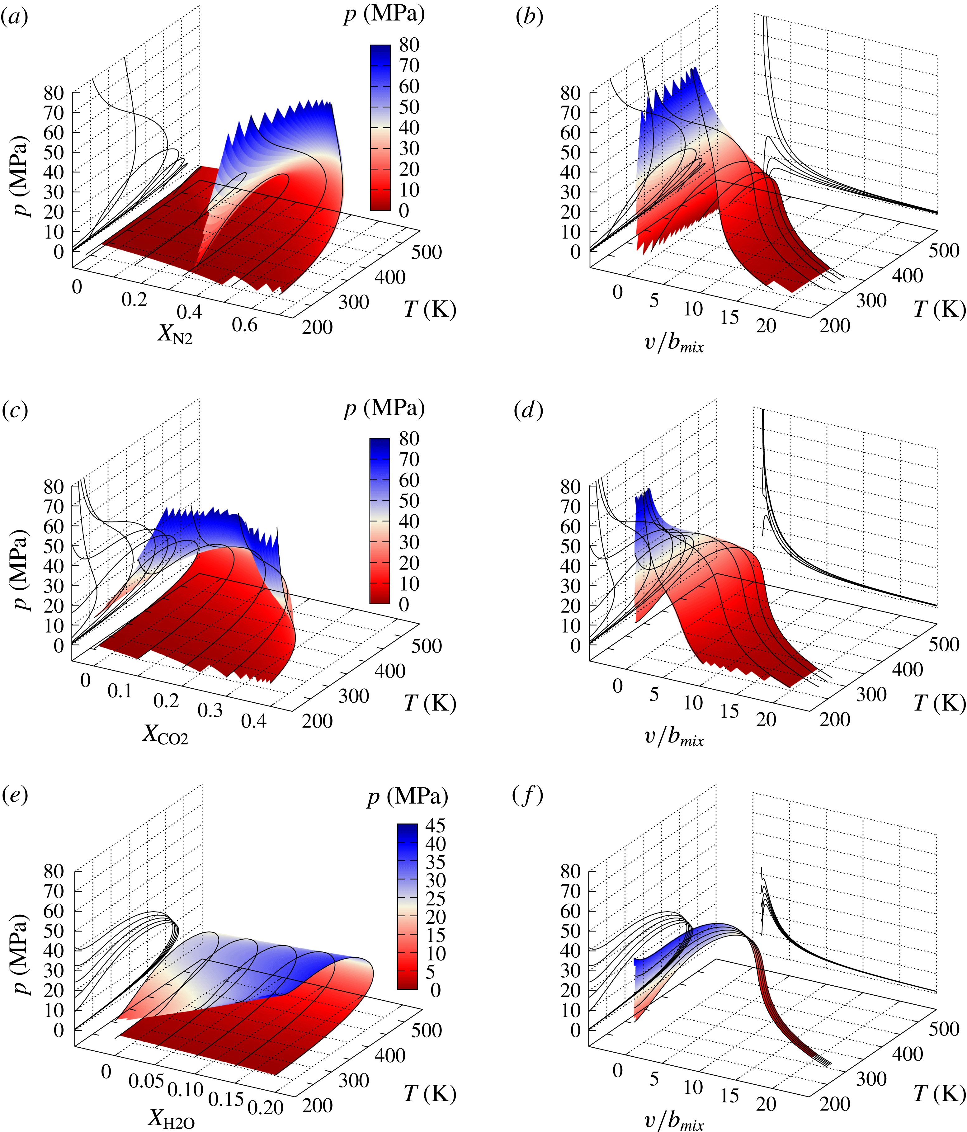
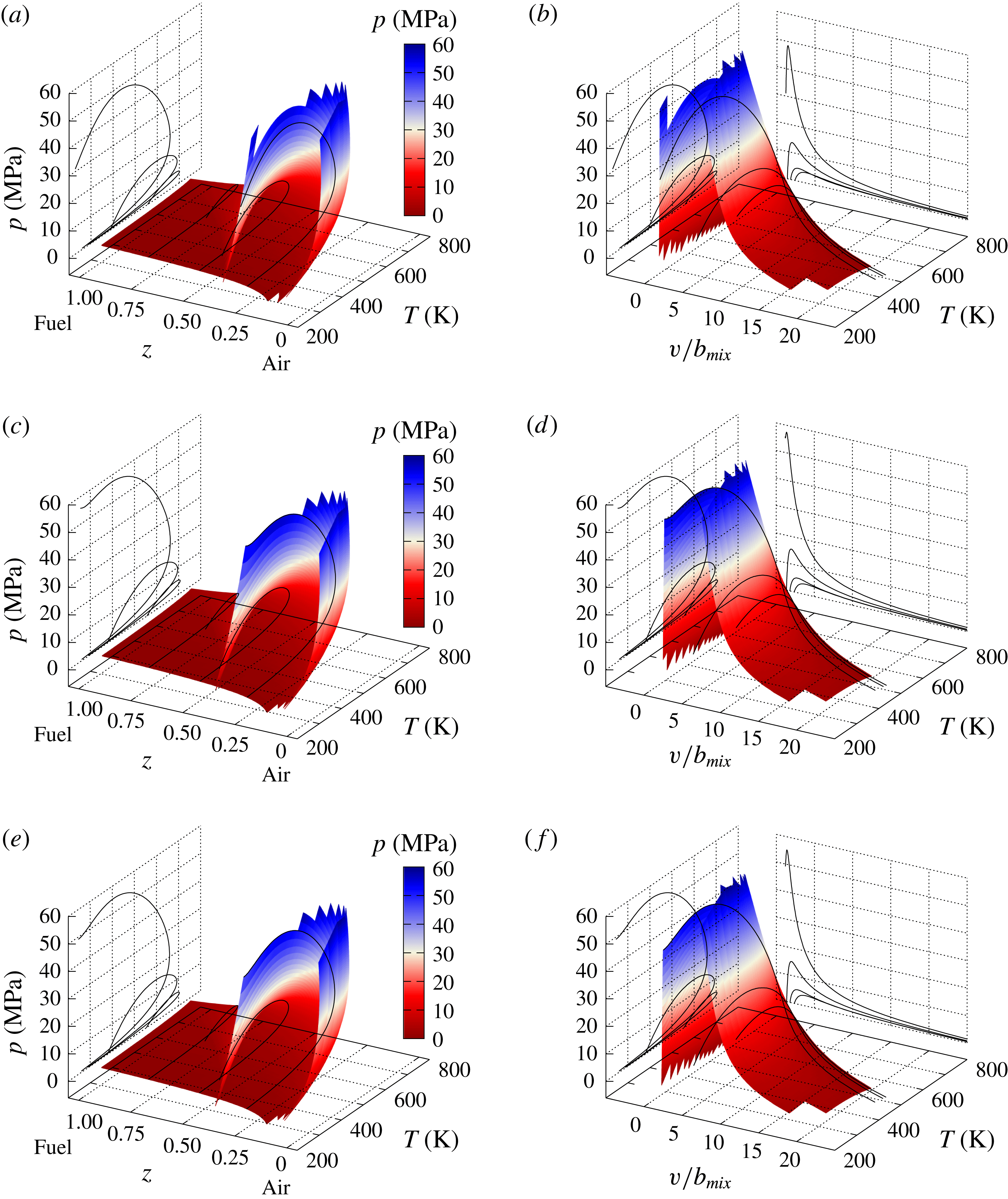
Spinodal locus of a five-species mixture: water, carbon dioxide, oxygen,
 $n$
-hexane and nitrogen. The molar fractions vary from
 $\{X_{\text{H2O}}=0.01,X_{\text{CO2}}=0.035,X_{\text{O2}}=0.1,X_{\text{C7H16}}=0,X_{\text{N2}}=0.855\}$
to
 $\{X_{\text{H2O}}=0.01,X_{\text{CO2}}=0.035,X_{\text{O2}}=0.1,X_{\text{C7H1}}=0.855,X_{\text{N2}}=0\}$
. The locus is shown in (a) the (
 $p,X_{\text{N2}},T$
) coordinates and (b) the (
 $p,v/b_{mix},T$
) coordinates. To visualize the shape of the surface,
 $(p,T)$
lines are plotted at fixed
 $X_{\text{N2}}$
. The colour legend of the locus according to the
 $p$
value only enables the topological features of the locus to be distinguished.

3.2 Spinodal locus of water, carbon dioxide, oxygen,
$n$
-heptane and nitrogen mixtures

An
 $\text{H}_{2}\text{O}$
,
 $\text{CO}_{2}$
,
 $\text{O}_{2}$
,
 $\text{C}_{7}\text{H}_{16}$
and
 $\text{N}_{2}$
mixture was used by Masi et al. (Reference Masi, Bellan, Harstad and Okong’o2013) and Bellan (Reference Bellan2017) in DNS studies of multispecies turbulent mixing and combustion, respectively, under high-
 $p$
conditions at
 $p=60$
and
 $80$
atm. An illustration of the spinodal locus for this mixture is given in figure 5(a), where
 $p$
is depicted as a function of
 $T$
and
 $X_{\text{N2}}$
for
 $X_{\text{H2O}}=0.01,X_{\text{CO2}}=0.035$
,
 $X_{\text{O2}}=0.1$
,
 $X_{\text{C7H16}}\in [0,0.855]$
and
 $X_{\text{N2}}\in [0.855,0];$
for completeness,
 $p$
values greatly in excess of those used in Masi et al. (Reference Masi, Bellan, Harstad and Okong’o2013) and Bellan (Reference Bellan2017) are shown, and for illustration purposes it is assumed that the PR EOS holds at those very large
 $p$
values. The values of
 $X_{\text{H2O}}$
and
 $X_{\text{CO2}}$
are representative of (but not the same as) the free-stream conditions of the mixing layer used in those studies. Spinodal curves at fixed
 $X_{\text{N2}}$
are visualized on the spinodal surface and on each one of the curves
 $X_{\text{H2O}}=0.01,X_{\text{CO2}}=0.035$
,
 $X_{\text{O2}}=0.1$
,
 $X_{\text{C7H16}}\in [0,0.855].$
These curves are projected in the
 $(p,T)$
plane and exhibit a wide variety of shapes. The same aspect of complex spinodal curves is exhibited in figure 5(b), where
 $p$
is shown versus
 $v/b_{mix}$
and
 $T,$
and the locus is visualized with curves at fixed
 $T$
that are projected in both the
 $(p,T)$
and
 $(p,v)$
planes. For each one of these curves, the composition is fixed. To further focus on identifying stable versus unstable thermodynamic regions, the spinodal curve intersection of
 $\{X_{\text{H2O}}=0.01,X_{\text{CO2}}=0.035,X_{\text{O2}}=0.1,X_{\text{C7H16}}=0.4,X_{\text{N2}}=0.455\}$
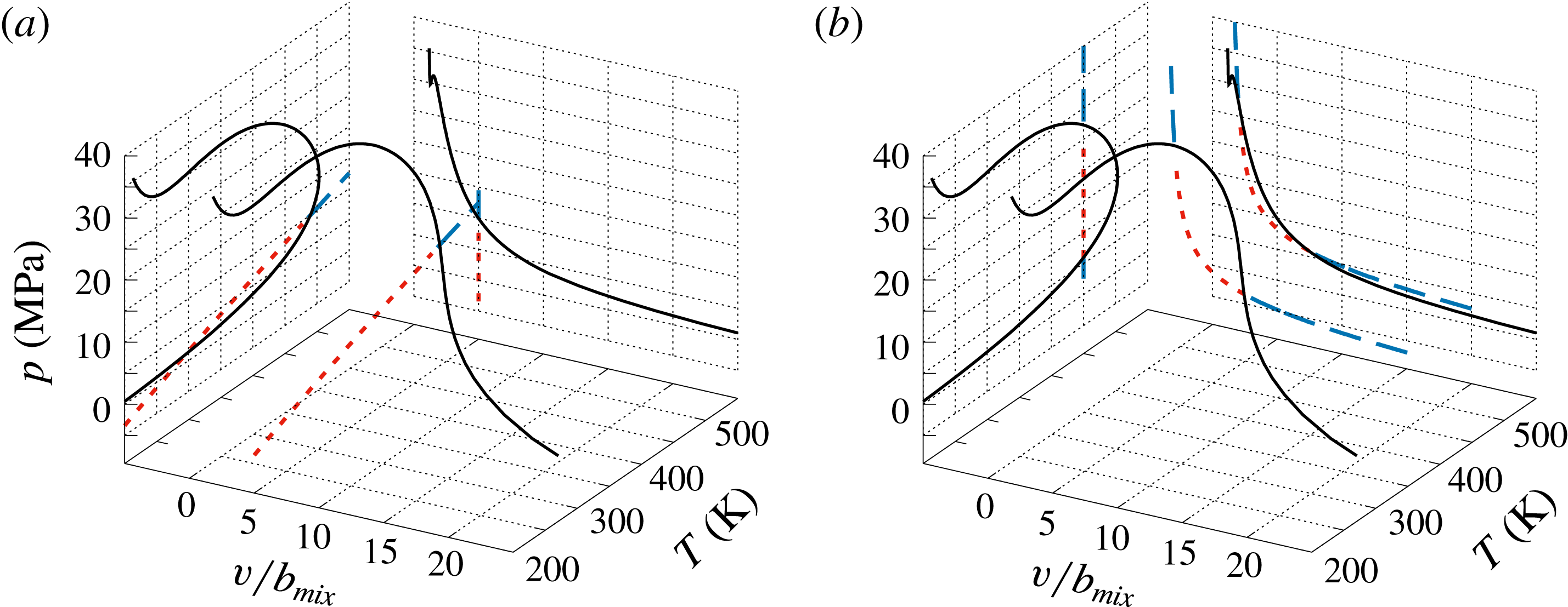
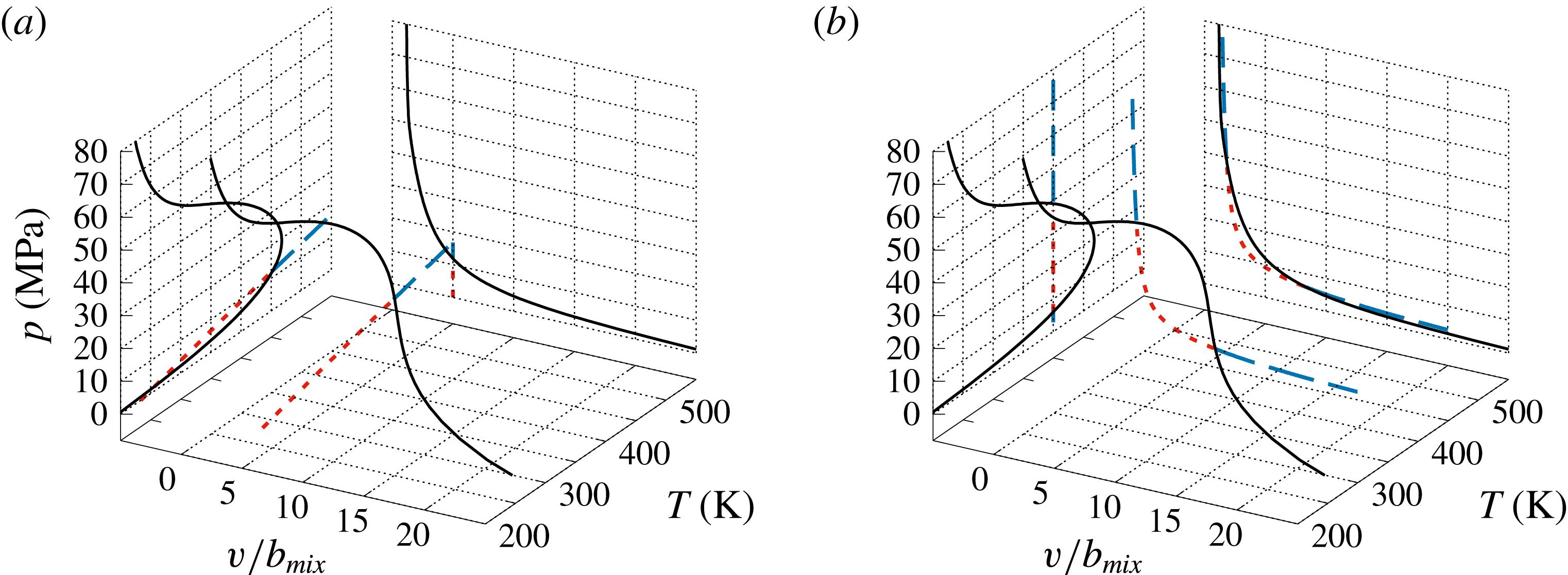
composition that appears in figure 5(b) is illustrated in figure 6(a) intersected by an isochore determined by
 $v/b_{mix}=5,$
and in figure 6(b) it is intersected by the
 $T=450~\text{K}$
isotherm, with projections of the spinodal curve in both the
 $(p,T)$
and
 $(p,v)$
planes also shown; the regions of stability and instability are clearly marked.
Spinodal curve of
 $\{X_{\text{H2O}}=0.01,X_{\text{CO2}}=0.035,X_{\text{O2}}=0.1,X_{\text{C7H16}}=0.4,X_{\text{N2}}=0.455\}$
composition and
 $T=450~\text{K}$
. (a) Spinodal curve intersected by an isochore and (b) spinodal curve intersected by an isotherm. Both isochore and isotherm are coloured according to the stability region: the - - - - and — — — lines represent unstable and stable regions respectively.

Having determined that the spinodal locus can be computed for this five-species system, it is now possible to use such calculations for examining the thermodynamic regime of the transitional states obtained by Masi et al. (Reference Masi, Bellan, Harstad and Okong’o2013) and Bellan (Reference Bellan2017), and of the peak-
 $p$
states obtained by Bellan (Reference Bellan2017).
3.3 Thermodynamic regimes of high-
$p$
multispecies turbulent flows from DNS databases

Evidence of uphill diffusion has been found during high-
 $p$
multispecies mixing through an a posteriori study of a DNS database (Masi et al.
Reference Masi, Bellan, Harstad and Okong’o2013) by accurately modelling and computing effective diffusion coefficients, some of which were negative at numerous locations in the domain (Masi et al.
Reference Masi, Bellan, Harstad and Okong’o2013). Similarly, an a posteriori analysis of DNS data from high-
 $p$
turbulent combustion also revealed evidence of uphill diffusion (Bellan Reference Bellan2017), in that regions where
 $\boldsymbol{J}_{\unicode[STIX]{x1D6FC}}\boldsymbol{\cdot }\unicode[STIX]{x1D735}Y_{\unicode[STIX]{x1D6FC}}>0$
, indicating uphill diffusion, were identified for the same species that exhibited negative effective diffusion coefficients during mixing.
The data of the simulations discussed in Masi et al. (Reference Masi, Bellan, Harstad and Okong’o2013) and Bellan (Reference Bellan2017) were obtained using the PR EOS in conjunction with a molar volume correction,
 $v_{s}$
, called a volume shift, for the purpose of enhancing accuracy (Harstad, Miller & Bellan Reference Harstad, Miller and Bellan1997). Consistency with the thermodynamic phase space map requires that the stability criteria be computed in the
 $(p,T,v_{PR},Y_{\unicode[STIX]{x1D6FC}})$
coordinates. The volume-shifted coordinates
 $(p,T,v,Y_{\unicode[STIX]{x1D6FC}})$
are extracted from the DNS database and
 $v_{PR}$
is then recovered using the following definitions:
 $$\begin{eqnarray}v_{PR}=v-v_{s},\quad v_{s}=\mathop{\sum }_{\unicode[STIX]{x1D6FC}=1}^{N}X_{\unicode[STIX]{x1D6FC}}\left[\frac{\unicode[STIX]{x2202}G_{\unicode[STIX]{x1D6FC}}^{0}}{\unicode[STIX]{x2202}p}\right]_{T},\end{eqnarray}$$
where
 $G$
is the Gibbs energy. Finally, the stability criterion is computed in the
 $(p,T,v_{PR},Y_{\unicode[STIX]{x1D6FC}})$
coordinates.
Following a preliminary analysis, the computation first addresses the species mixing DNS database (Masi et al. Reference Masi, Bellan, Harstad and Okong’o2013) and is then applied to the reactive flow DNS database (Bellan Reference Bellan2017).
3.3.1 Preliminary analysis of potential thermodynamic states in the mixing layer
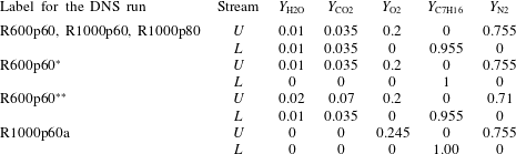
Towards the goal of determining the thermodynamic regime of the transitional states obtained during mixing and combustion of five species in a mixing layer configuration (Masi et al. Reference Masi, Bellan, Harstad and Okong’o2013; Bellan Reference Bellan2017), some preliminary evaluations may be performed without consideration of these transitional states and only based on the free-stream compositions. Three of the simulations from Masi et al. (Reference Masi, Bellan, Harstad and Okong’o2013) and one simulation from Bellan (Reference Bellan2017) are analysed in these preliminary evaluations; their thermodynamic free-stream conditions are listed in table 4.
Initial mass fractions of water, carbon dioxide, oxygen,
 $n$
-heptane and nitrogen in the upper (
 $U$
) and lower (
 $L$
) streams. In all simulations,
 $T_{L}=600~\text{K}$
and
 $T_{U}=1000~\text{K}$
. Here, R denotes the initial Reynolds number value,
 $Re_{0}$
, as defined in Masi et al. (Reference Masi, Bellan, Harstad and Okong’o2013) and p denotes the free-stream pressure in atm, e.g. R1000p60 labels a simulation in which
 $Re_{0}=1000$
and
 $p_{0}=60$
atm.

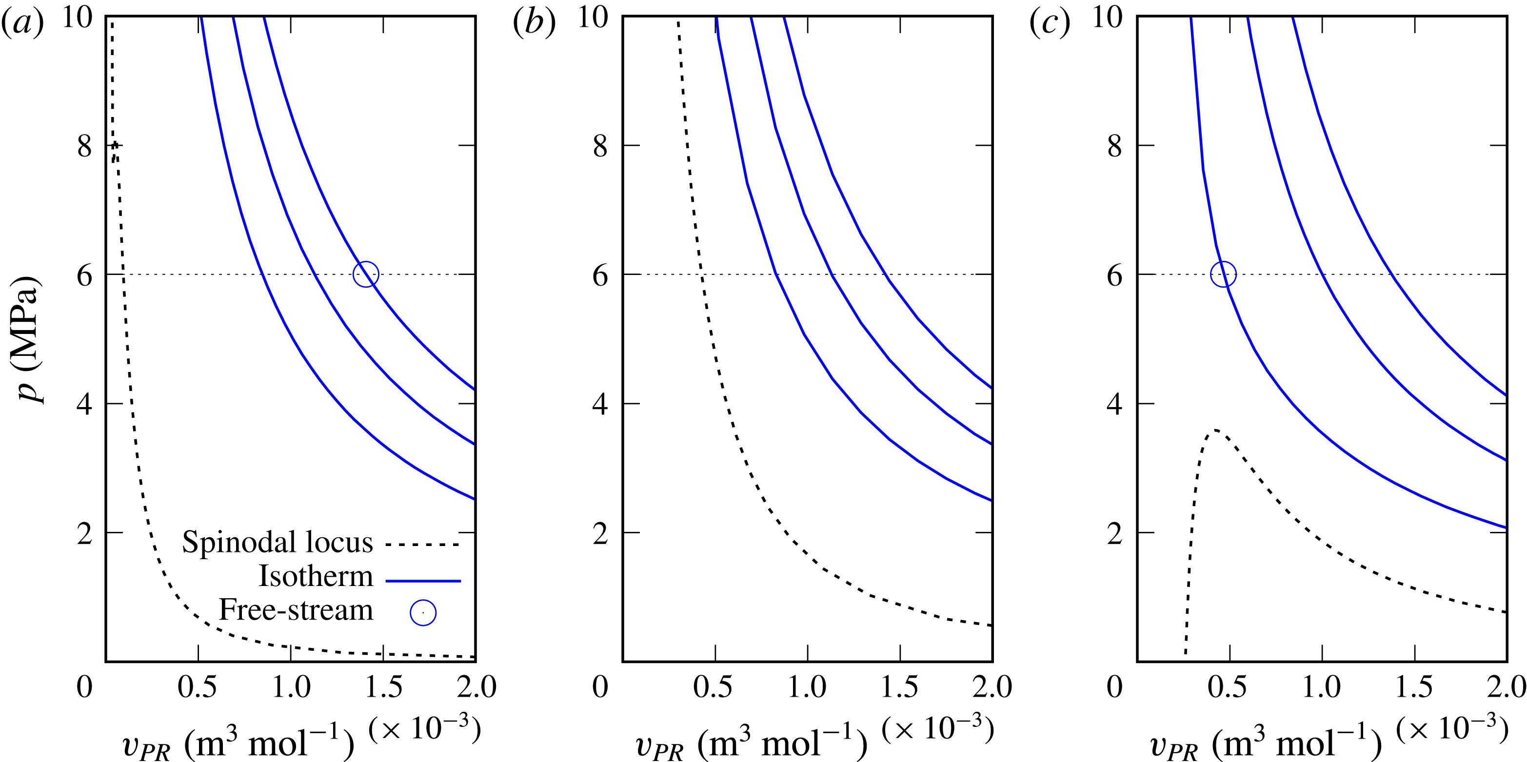
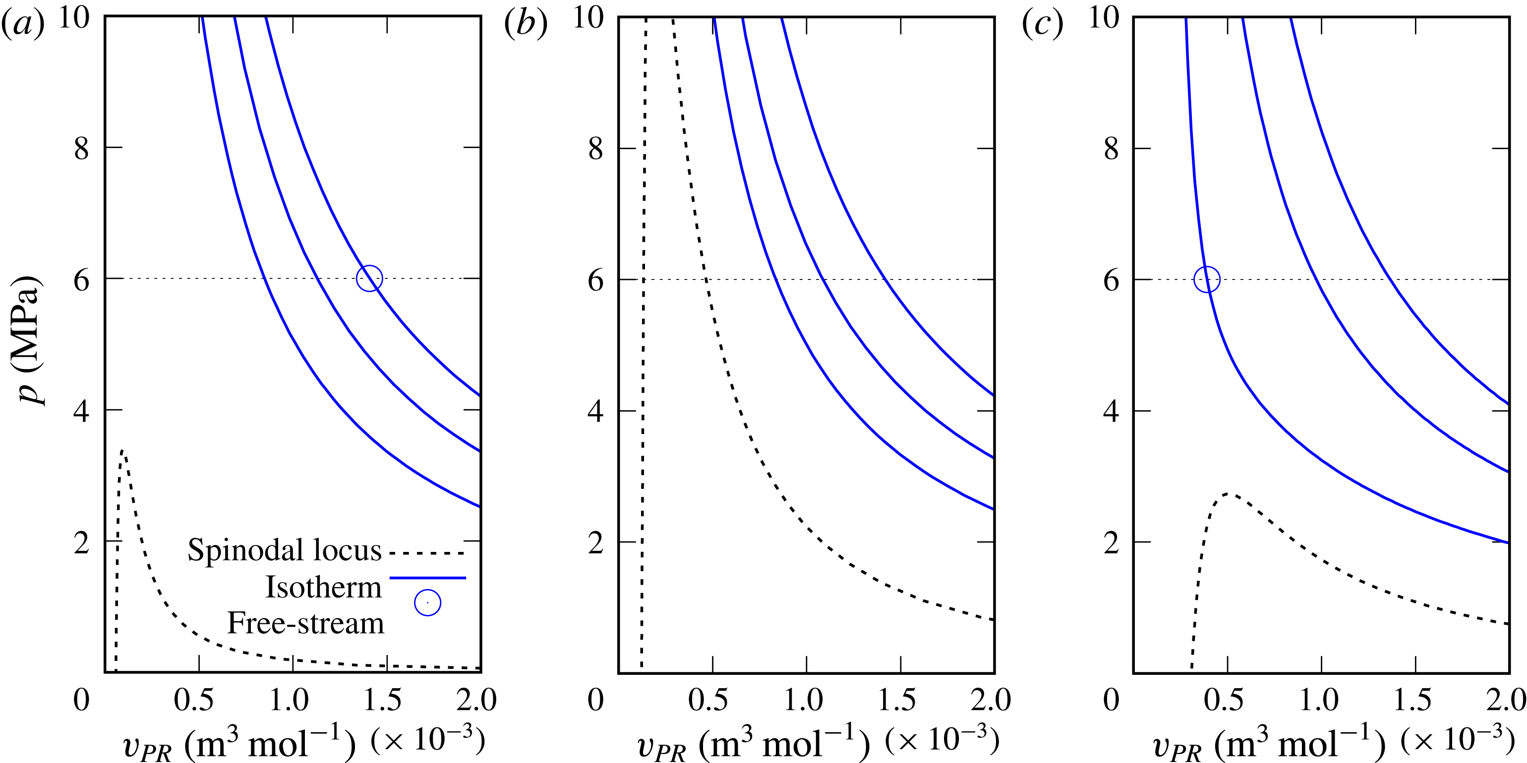
Mixing layer free-stream thermodynamic conditions (circle) plotted with their respective spinodal locus (dashed line) for the R600p60 case. Three isotherms are plotted for
 $T=600,800,1000~\text{K}$
(solid line). (a) The conditions are those in the upper stream; (b) the conditions are obtained by a linear interpolation between those of the upper and lower streams; (c) the conditions are those of the lower stream.

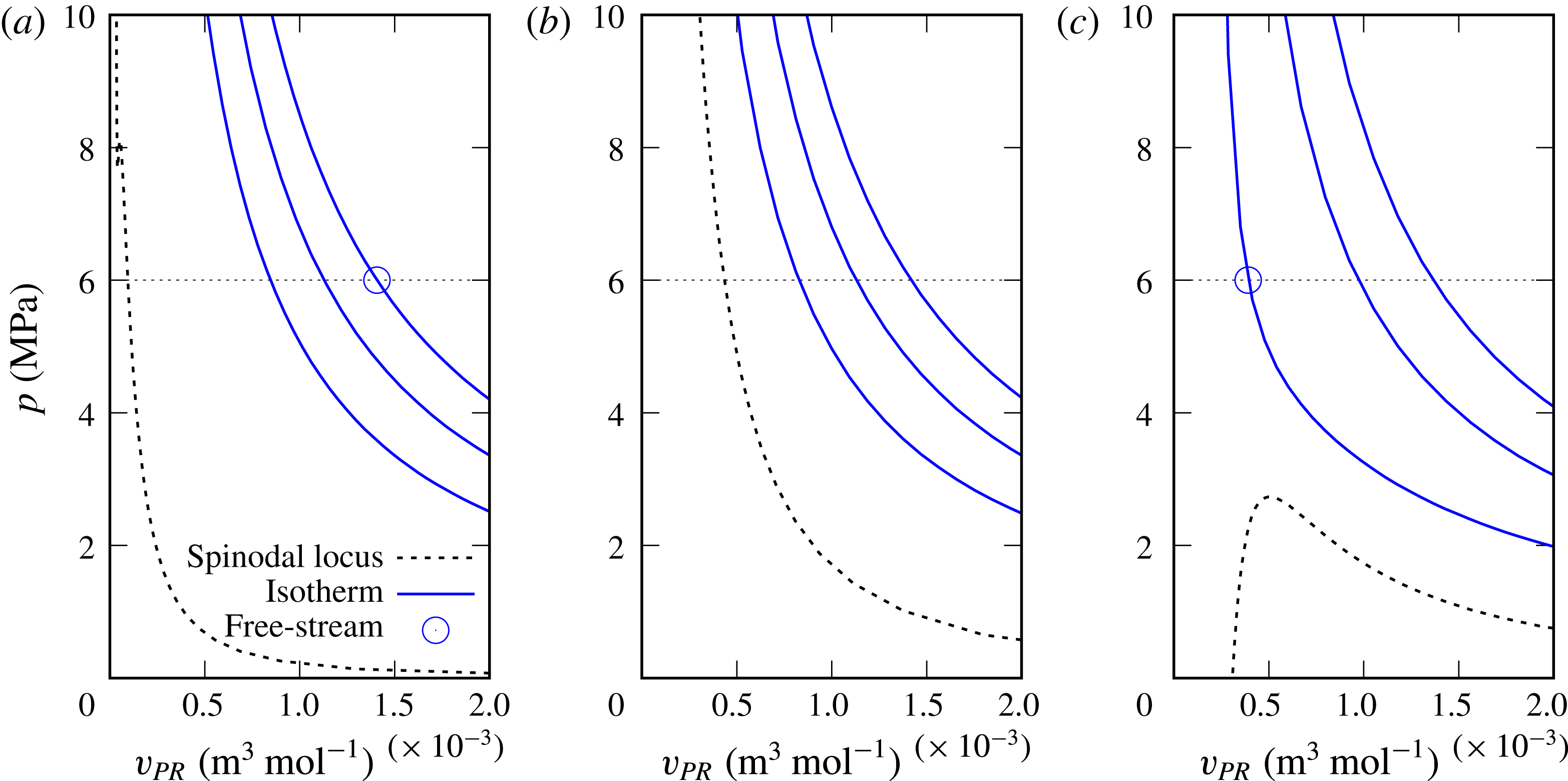
Mixing layer free-stream thermodynamic conditions (circle) plotted with their respective spinodal locus (dashed line) for the R600p60* case. Three isotherms are plotted for
 $T=600,800,1000~\text{K}$
(solid line). (a) The conditions are those in the upper stream; (b) the conditions are obtained by a linear interpolation between those of the upper and lower streams; (c) the conditions are those of the lower stream.

In a very approximative manner, it could be expected that during the layer evolution there will be some locations where the composition is the arithmetic average of the upper and lower free-stream compositions; the same argument applies to
 $T$
, which is expected to be
 $T\in [600,1000]~\text{K}$
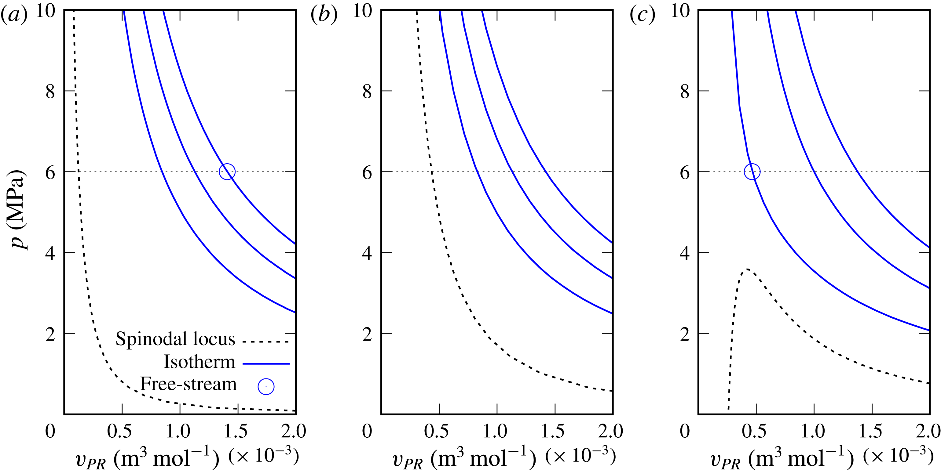
. In figures 7–10, the spinodal locus and the free-stream thermodynamic conditions together with three isotherms (with
 $T=600,800,1000~\text{K}$
) are illustrated. Figures 7–10 illustrate results based on the initial conditions R600p60, R600p60*, R600p60** and R1000p60a, respectively. Figures 7(a)–10(a) show the spinodal locus representing the upper stream conditions, figures 7(b)–10(b) exhibit the spinodal locus together with the three isotherms for a mixture composition which is the arithmetic average of the upper and lower streams, while figures 7(c)–10(c) display the locus corresponding to the lower stream. Since it appears in figures 7–10 that both the free-stream conditions and the isotherms are above the spinodal locus, this simple estimate indicates that it is unlikely that spinodal decomposition would occur. However, due to differential diffusion effects among species, the mass fractions cannot be expected to be simply the arithmetic averages of the two free-stream conditions. For this reason, no definitive conclusions can be inferred from this preliminary analysis, and the results of the databases must be interrogated instead.
Mixing layer free-stream thermodynamic conditions (circle) plotted with their respective spinodal locus (dashed line) for the R600p60** case. Three isotherms are plotted for
 $T=600,800,1000~\text{K}$
(solid line). (a) The conditions are those in the upper stream; (b) the conditions are obtained by a linear interpolation between those of the upper and lower streams; (c) the conditions are those of the lower stream.

Mixing layer free-stream thermodynamic conditions (circle) plotted with their respective spinodal locus (dashed line) for the R1000p60a case. Three isotherms are plotted for
 $T=600,800,1000~\text{K}$
(solid line). (a) The conditions are those in the upper stream; (b) the conditions are obtained by a linear interpolation between those of the upper and lower streams; (c) the conditions are those of the lower stream.

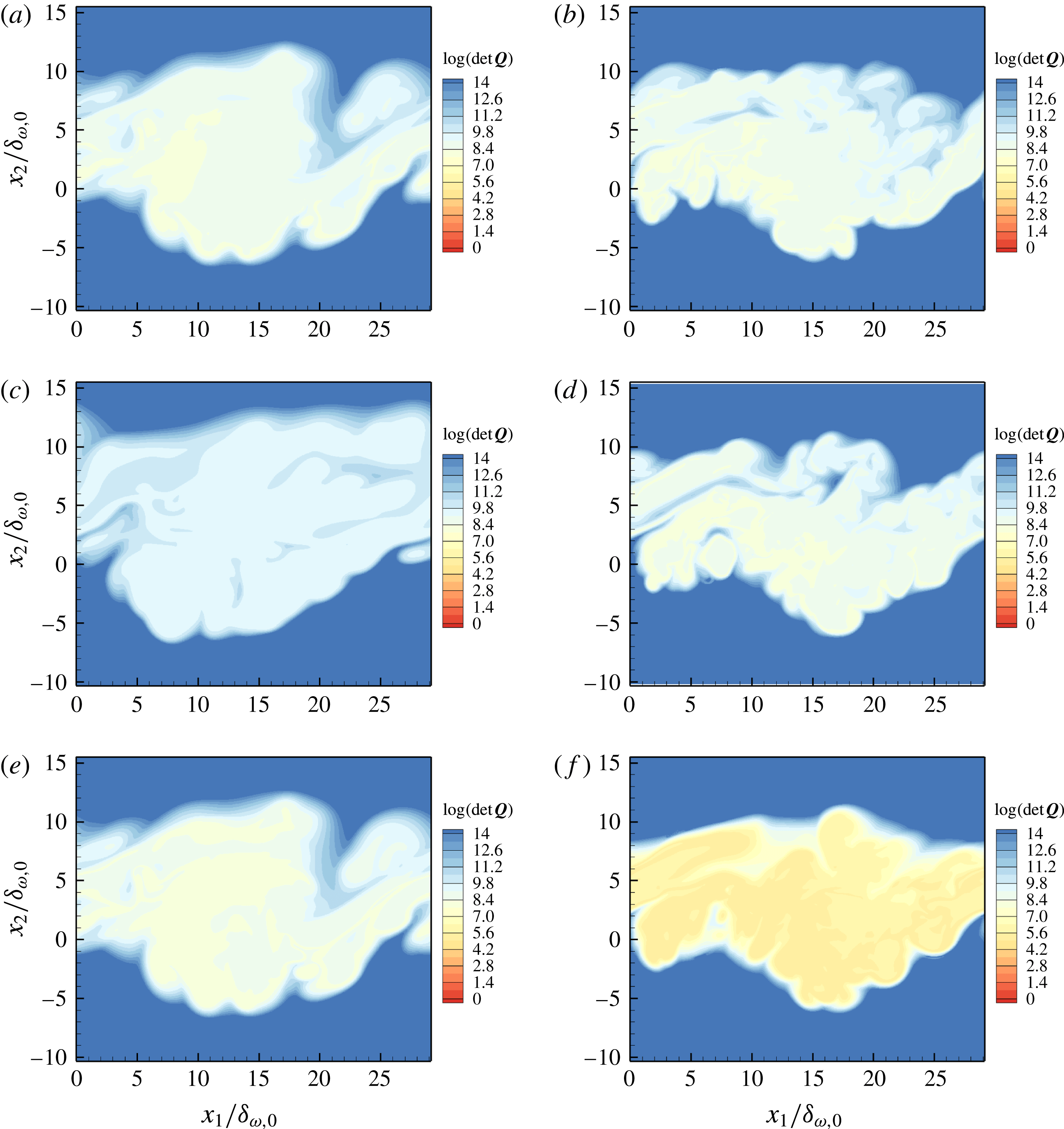
 $\text{Log}(\det \boldsymbol{Q})$
, where the matrix elements are computed according to (2.14) for the simulations listed in table 4 at time
 $t_{tr}^{\ast }$
for each simulation and in the plane
 $x_{3}/L_{3}=0$
: (a) R600p60, (b) R1000p60, (c) R600p60
 $^{\ast }$
, (d) R1000p80, (e) R600p60
 $^{\ast \ast }$
, (f) R1000p60a.

3.3.2 Analysis of the database for species mixing
The thermodynamic regime of transitional states obtained during mixing is here determined by analysing the database obtained in Masi et al. (Reference Masi, Bellan, Harstad and Okong’o2013) from DNS of the R600p60, R1000p60, R1000p80, R600p60* and R600p60** cases listed in table 4, representing the mixing of five species, and the transitional state of the R1000p60a DNS from Bellan (Reference Bellan2017) that, unlike the other five cases, represents the mixing of only three species. The mixing layer of coordinates
 $(x_{1},x_{2},x_{3})$
has dimensions
 $(L_{1},L_{2},L_{3}).$
The initial Reynolds number is defined as
 $Re_{0}\equiv [0.5(\unicode[STIX]{x1D70C}_{U}+\unicode[STIX]{x1D70C}_{L})\unicode[STIX]{x0394}U_{0}\unicode[STIX]{x1D6FF}_{\unicode[STIX]{x1D714},0}]/\unicode[STIX]{x1D707}_{R}$
, where
 $\unicode[STIX]{x1D70C}_{U}$
and
 $\unicode[STIX]{x1D70C}_{L}$
are mixture initial densities and
 $U$
and
 $L$
subscripts label the upper and lower streams;
 $\unicode[STIX]{x1D6FF}_{\unicode[STIX]{x1D714},0}=\unicode[STIX]{x0394}U_{0}/(\unicode[STIX]{x2202}u_{0}/\unicode[STIX]{x2202}x_{2})_{max}$
is the initial vorticity thickness computed by using
 $u_{0}$
, which is the
 $(x_{1},x_{3})$
planar average of the initial velocity in the streamwise direction;
 $\unicode[STIX]{x0394}U_{0}=U_{U}-U_{L}$
is the initial velocity difference across the layer;
 $\unicode[STIX]{x1D707}_{R}$
is a reference viscosity (see in Masi et al. (Reference Masi, Bellan, Harstad and Okong’o2013) a discussion regarding the
 $\unicode[STIX]{x1D707}_{R}$
calculation). Each simulation is pursued to a transitional state defined as occurring at a time
 $t_{tr}^{\ast }$
when the one-dimensional fluctuation-based spectra of the dynamic and thermodynamic variables are smooth. For each of the transitional states, at each grid point in the domain,
 $\det \boldsymbol{Q}$
is computed according to the methodology described and validated in § 2.2. The results in a selected spanwise plane,
 $x_{3}/L_{3}=0,$
are displayed in figure 11.


These results show that, irrespective of the initial conditions, the flow in the mixing layer is in the single-phase regime. When uphill diffusion does not occur (i.e. R600p60
 $^{\ast }$
), the flow is slightly further away in the single-phase regime from the spinodal locus, as indicated by the larger values of
 $\det \boldsymbol{Q}$
compared with the simulations in which uphill diffusion occurs. That is, despite the strong compositional variations in the mixing layer and despite the different spatiotemporal evolutions of the simulations listed in table 4, for this range of
 $(p,T)$
conditions, mixtures of these five species are in the single-phase regime.
3.3.3 Analysis of the database for reacting species
A similar analysis to that of § 3.3.2 is here performed to understand the thermodynamic regime during combustion. In these DNS, the reaction is initiated at the transitional state obtained during mixing, and the computation is continued past a state, at
 $t_{pp}^{\ast }$
, at which the pressure peaks. The database used for the analysis is that obtained at
 $t_{pp}^{\ast }$
, and described in detail in Bellan (Reference Bellan2017). The four DNS conducted in that study are here analysed and the respective initial conditions are shown in table 4. Both
 $T$
and
 $p$
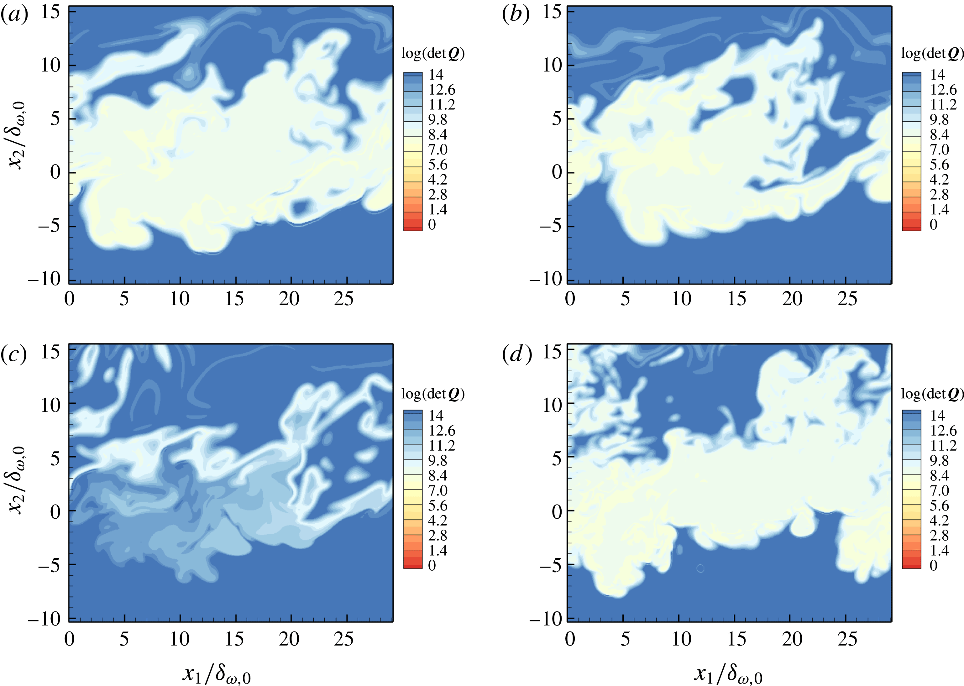
are larger during combustion than during mixing, and thus the expectation is that the mixture will be further from the spinodal locus in the single-phase regime than in figure 11. Figure 12 displays
 $\det \boldsymbol{Q}$
obtained for the combustion database and indeed shows that compared with the respective cases in figure 11, this expectation is confirmed by the stability computations. It is of note, as expected, for R1000p60a, for which the reaction rate is more intense (because there are initially more reactants) since
 $\text{CO}_{2}$
and
 $\text{H}_{2}\text{O}$
are not initially present, that the value of
 $\det \boldsymbol{Q}$
is larger, a fact that is attributed to the higher energy release conjectured to lead to a larger
 $T$
.
4 Spinodal locus calculation for understanding practical-fuel injection and mixing
Currently, the controversy over whether the species mixture in high-
 $p$
combustion devices is in the single-phase or two-phase regime is based on experimental data that do not necessarily portray the compositional complexity of those mixtures and/or are performed with chemical species uncharacteristic of those mixtures. The above results showed that the spinodal locus is a function of both the complexity of the mixture and the mixture specific composition. The local microscopic composition may be changed by diffusion, solubility or reactions, whereas the macroscopic composition is also subject to turbulent conditions. However, for non-reactive flows, existing experimental data relevant to high-
 $p$
species mixing are primarily limited to binary-species mixing, for which the phenomenon of uphill diffusion cannot be observed since the diffusion matrix is
 $2\times 2$
and it is populated with binary-diffusion coefficients, all of which, according to established physics, are positive or null. Such existing experiments observe a jet injected into a chamber of different composition from the jet. Notable experiments have been performed for LOX into
 $\text{H}_{2}$
(Mayer & Tamura Reference Mayer and Tamura1996; Mayer et al.
Reference Mayer, Schik, Schweitzer and Schaeffler1996), LOX into
 $\text{N}_{2}$
(Chehroudi, Talley & Coy Reference Chehroudi, Talley and Coy2002),
 $\text{N}_{2}$
into
 $\text{N}_{2}$
(Oschwald & Schik Reference Oschwald and Schick1999; Chehroudi et al.
Reference Chehroudi, Talley and Coy2002),
 $\text{N}_{2}$
into
 $\text{H}_{2}$
(Oschwald et al.
Reference Oschwald, Schik, Klar and Mayer1999), He into
 $\text{N}_{2}$
(Chehroudi et al.
Reference Chehroudi, Talley and Coy2002),
 $\text{N}_{2}$
into He (Chehroudi et al.
Reference Chehroudi, Talley and Coy2002), a fluoroketone into
 $\text{N}_{2}$
(Roy, Clement Joly & Corin Segal Reference Roy, Clement Joly and Corin Segal2013), and butanol,
 $n$
-dodecane or
 $n$
-hexadecane into
 $\text{N}_{2}$
(Falgout et al.
Reference Falgout, Rahm, Sedarsky and Linne2016). A few exceptions from the binary-species conditions exist, but they are not sufficiently quantitatively documented for comparisons with simulations to be attempted. For example, regarding specific mixture compositions,
 $\text{N}_{2}$
was injected into 10 % CO and 90 %
 $\text{N}_{2}$
(Chehroudi et al.
Reference Chehroudi, Talley and Coy2002), but only limited jet spreading information is available. Additionally, Crua et al. (Reference Crua, Manin and Pickett2017) injected
 $n$
-heptane,
 $n$
-dodecane or
 $n$
-hexadecane into a mixture of
 $\text{C}_{2}\text{H}_{2}$
,
 $\text{H}_{2}$
,
 $\text{N}_{2}$
and
 $\text{O}_{2}$
of indefinite composition, while Crua et al. (Reference Crua, Heikal and Gold2015) used a rapid compression machine to inject fuels of uncertain composition (e.g. diesel, kerosene) into air. The importance of the quantitative knowledge of the injected-mixture composition for determining the thermodynamic regime was highlighted by Falgout et al. (Reference Falgout, Rahm, Sedarsky and Linne2016), and of course the same holds for the mixture into which injection occurs. The results of § 2 support the assertion that knowledge of the composition is essential in these calculations. We show below that it is possible to compute and visualize the spinodal locus for a variety of mixtures, most of which are considerably more compositionally complex than the five-species mixture considered in §§ 3.3.2 and 3.3.3. This information leads to determination of the thermodynamic regime of practical fuels immediately upon injection into a combustion chamber and during mixing prior to ignition.
4.1 A mixture of two
$n$
-alkanes and nitrogen

The spinodal locus of a mixture of
 $n$
-hexane (1),
 $n$
-heptane (2) and nitrogen (3) computed using the method of § 2.2 is illustrated in figure 13, showing
 $p$
as a function of
 $T$
and
 $X_{\text{N2}}$
in figure 13(a) and as a function of
 $T$
and
 $v/b_{mix}$
in figure 13(b). The molar fractions are varied in the interval
 $\{X_{\text{C6H14}}=0.5,X_{\text{C7H16}}=X_{\text{C6H14}},X_{\text{N2}}=0\}$
–
 $\{X_{\text{C6H14}}=0.1,X_{\text{C7H16}}=X_{\text{C6H14}},X_{\text{N2}}=0.8\}$
. In figure 13(a), the projections of the spinodal at fixed
 $X_{\text{N2}}$
are presented in the
 $(p,T)$
plane, and it appears that these curves have a variety of shapes. To aid the visualization of the spinodal locus shape, in figure 13(b), the same surface and lines at constant composition as in figure 13(a) are plotted in the
 $(p,T,v/b_{mix})$
coordinates. The spinodals at constant composition are projected onto the
 $(p,v)$
and
 $(p,T)$
planes as well.
Spinodal locus of the ternary mixture
 $n$
-hexane (1),
 $n$
-heptane (2) and nitrogen (3) over the composition interval
 $\{X_{1}=0.5,X_{2}=X_{1},X_{3}=0\}$
–
 $\{X_{1}=0.1,X_{2}=X_{1},X_{3}=0.8\}$
. The locus is visualized in (a)
 $(p,X_{\text{N2}},T)$
coordinates and (b)
 $(p,v/b_{mix},T)$
coordinates. To visualize the shape of the surface,
 $(p,T)$
lines are plotted at fixed
 $X_{\text{N2}}$
. The colour legend of the locus according to the
 $p$
value only enables the topological features of the locus to be distinguished.

Spinodal locus of the ternary mixture
 $n$
-hexane (1),
 $n$
-heptane (2) and nitrogen (3) at fixed composition
 $\{X_{1}=0.4,X_{2}=X_{1},X_{3}=0.2\}$
. (a) Isochore intersecting the spinodal locus and (b) isotherm intersecting the spinodal locus. Projections are shown on the
 $(p,T)$
and
 $(p,v)$
planes. Both unstable (- - - -) and stable (— — —) regimes are indicated on the isochore, isotherm and their projections.

The regions of stability and instability are indicated in figure 14(a) on the isochore
 $v/b_{mix}=10$
and in figure 14(b) on the isotherm
 $T=400~\text{K}$
, each intersecting with the spinodal curve defined by
 $\{X_{\text{C6H14}}=0.4,X_{\text{C7H16}}=X_{\text{C6H14}},X_{\text{N2}}=0.2\}$
and
 $T=450~\text{K}$
. It is of note that projections of the spinodal locus in a plane can be deceiving because they lack the three-dimensionality that imparts the full characteristics of the physics; these projections may erroneously lead one, for example, to consider that a curve exhibits a loop as it intersects itself, whereas in reality such intersection does not occur.
4.2 Complex fuels mixed with air:
$n$
-hexane,
$n$
-heptane, nitrogen, oxygen and other light species


In principle, spinodal locus calculations, from which we infer stability or instability, can be performed for a mixture having an arbitrary number of species; the limitation is the availability of data for the binary interaction parameters in the EOS. The present mixture is sufficiently complex – twelve species – to be representative, as far as the number of species, of a reduced chemical kinetics mechanism (excluding radicals). The mixture is composed of
 $n$
-hexane (1),
 $n$
-heptane (2), nitrogen (3), oxygen (4), carbon dioxide (5), carbon oxide, CO (6), water (7), hydrogen peroxide,
 $\text{H}_{2}\text{O}_{2}$
(8), hydrogen (9), methane (10), ethyne,
 $\text{C}_{2}\text{H}_{2}$
(i.e. acetylene) (11), and ethene,
 $\text{C}_{2}\text{H}_{6}$
(i.e. ethylene) (12). For the spinodal locus calculation, three composition variations are considered. The results obtained by varying the composition from
 $\{X_{1}=0.05,X_{2}=X_{1},X_{3}=0.7,X_{4}=0.05,X_{5}=0.045,X_{6}=X_{7}=X_{8}=X_{9}=X_{10}=X_{11}=X_{12}=0.015\}$
to
 $\{X_{1}=0.4,X_{2}=X_{1},X_{3}=0.0,X_{4}=0.05,X_{5}=0.045,X_{6}=X_{7}=X_{8}=X_{9}=X_{10}=X_{11}=X_{12}=0.015\}$
, i.e.
 $X_{4}$
–
 $X_{12}$
are kept constant, are illustrated in figure 15(a,b) in
 $(p,T,X_{\text{N2}})$
and
 $(p,T,v/b_{mix})$
systems of coordinates. For the composition variation in the
 $\{X_{1}=0.0,X_{2}=X_{1},X_{3}=0.395,X_{4}=0.1,X_{5}=0.4,X_{6}=X_{7}=X_{8}=X_{9}=X_{10}=X_{11}=X_{12}=0.015\}$
–
 $\{X_{1}=0.2,X_{2}=X_{1},X_{3}=0.395,X_{4}=0.1,X_{5}=0.0,X_{6}=X_{7}=X_{8}=X_{9}=X_{10}=X_{11}=X_{12}=0.015\}$
range, the corresponding locus is depicted in figure 15(c) in
 $(p,T,X_{\text{CO2}})$
coordinates and in figure 15(d) which shows the locus in
 $(p,T,v/b_{mix})$
coordinates. A third spinodal locus spanning the composition range
 $\{X_{1}=0.2,X_{2}=X_{1},X_{3}=0.38,X_{4}=0.1,X_{5}=0.03,X_{6}=0.0,X_{7}=X_{8}=X_{9}=X_{10}=X_{11}=X_{12}=0.015\}$
–
 $\{X_{1}=0.16,X_{2}=X_{1},X_{3}=0.304,X_{4}=0.08,X_{5}=0.024,X_{6}=0.2,X_{7}=X_{8}=X_{9}=X_{10}=X_{11}=X_{12}=0.012\}$
is shown in the systems of coordinates
 $(p,T,X_{\text{H2O}})$
and
 $(p,T,v/b_{mix})$
in figures 15(e) and 15(f), respectively. In each case, the locus is visualized by a
 $p$
-colour legend (different
 $p$
values correspond to the colours for each panel of figure 15), by curves of constant
 $X_{\unicode[STIX]{x1D6FC}}$
and by projections in the
 $(p,T)$
plane (figure 15
a–f) and in the
 $(p,v)$
plane (figure 15
b,d,f). As expected, but typically not shown, with increasing species in the mixture, the locus becomes more complex and assumes a variety of shapes when visualized as a function of different
 $X_{\unicode[STIX]{x1D6FC}}$
. To further clarify the regions of stability and instability, a single curve of the locus corresponding to the
 $\{X_{1}=0.15,X_{2}=X_{1},X_{3}=0.5,X_{4}=0.15,X_{5}=0.045,X_{6}=X_{7}=X_{8}=X_{9}=X_{10}=X_{11}=X_{12}=0.015\}$
composition and to
 $T=300~\text{K}$
is exhibited in figure 16(a) as intersected by the isochore
 $v/b_{mix}=5$
and in figure 16(b) as intersected by the isotherm
 $T=400~\text{K}$
.
Spinodal locus of a twelve-species mixture:
 $n$
-hexane,
 $n$
-heptane, nitrogen, oxygen, carbon dioxide, carbon oxide, water, hydrogen peroxide, hydrogen, methane, ethyne (i.e. acetylene) and ethene (i.e. ethylene): (a,c,e)
 $(p,T,X_{\text{N2}})$
,
 $(p,T,X_{\text{CO2}})$
and
 $(p,T,X_{\text{H2O}})$
loci showing curves at constant
 $X_{\text{N2}}$
,
 $X_{\text{CO2}}$
and
 $X_{\text{H2O}}$
, respectively, that are projected onto the
 $(p,T)$
plane; (b,d,f)
 $(p,T,v/b_{mix})$
locus including projections onto the
 $(p,T)$
and
 $(p,v/b_{mix})$
planes. The colour legend of the locus according to the
 $p$
value only enables the topological features of the locus to be distinguished.

Spinodal locus of a duodenary mixture:
 $n$
-hexane (1),
 $n$
-heptane (2), nitrogen (3), oxygen (4), carbon dioxide (5), carbon oxide, CO (6), water (7), hydrogen peroxide,
 $\text{H}_{2}\text{O}_{2}$
(8), hydrogen (9), methane (10), ethyne,
 $\text{C}_{2}\text{H}_{2}$
(i.e. acetylene) (11), and ethene,
 $\text{C}_{2}\text{H}_{6}$
(i.e. ethylene) (12). The molar fraction composition is
 $\{X_{1}=0.15,X_{2}=X_{1},X_{3}=0.5,X_{4}=0.15,X_{5}=0.045,X_{6}=X_{7}=X_{8}=X_{9}=X_{10}=X_{11}=X_{12}=0.015\}$
and
 $T=300~\text{K}$
. (a) Spinodal locus intersected by an isochore and projected onto the
 $(p,T)$
plane; (b) spinodal locus intersected by an isotherm and projected onto the
 $(p,v)$
plane. The stability (— — —) and instability (- - - -) regions are indicated on the isochore, isotherm and on their projections.

4.3 Diesel fuels
Ultimately, the interest is in determining the thermodynamic regime of injected diesel fuels at different stages of their spatiotemporal evolution in a high-
 $p$
combustion chamber environment. Immediately upon injection, the diesel-fuel species-mixture pristine composition will be exposed to the
 $(p,T,X_{\unicode[STIX]{x1D6FC}})$
conditions of the chamber. As already stated, as time evolves and before ignition, there are two phenomena which may change the microscopic composition of the injected mixture: diffusion of species and solubility effects. Diffusion is a slow process which becomes even slower as
 $p$
increases. On the contrary, solubility increases with
 $p$
, and it is thus conceivable that species from the mixture in the chamber may dissolve into the fuel mixture before ignition occurs. For this reason, the spinodal loci of several known compositions of diesel fuels are here computed, and each composition is considered as an initial condition, leading to other possible compositions containing a certain percentage of air which is the typical chamber occupant.
Three different diesel surrogates, labelled V0a, V0b and V1 in Mueller et al. (Reference Mueller, Cannella, Bays, Bruno, DeFabio, Dettman, Gieleciak, Huber, Kweon and McConnell2016), of increasing complexity have been investigated that contain respectively four, five and eight components; the compositions of these surrogates are listed in table 5.
Three diesel-fuel surrogate compositions from Mueller et al. (Reference Mueller, Cannella, Bays, Bruno, DeFabio, Dettman, Gieleciak, Huber, Kweon and McConnell2016).

The spinodal loci of air/diesel-surrogate mixtures: (a,b) V0a, (c,d) V0b, (e,f) V1; the compositions of these fuel mixtures are listed in table 5. For all panels,
 $(p,T)$
lines at constant mixture fraction are plotted to clarify the shape of the surface and projected on the
 $(p,T)$
plane; for panels (b,d,f) projections onto the
 $(p,v/b_{mix})$
plane are shown as well. The colour legend of the locus according to the
 $p$
value only enables the topological features of the locus to be distinguished.

The spinodal loci are computed as a function of the fuel mole fraction in the mixture,
 $z$
, so that
 $z=1$
corresponds to pure fuel and
 $z=0$
corresponds to pure air, as can be seen in figure 17. The first mixture (air–V0a) is composed of nitrogen, oxygen and the species listed under V0a in table 5, and
 $z=\sum _{\unicode[STIX]{x1D6FC}=3}^{6}X_{\unicode[STIX]{x1D6FC}}$
. The composition variation on the locus is from pure fuel
 $\{\!X_{1}=X_{2}=0,X_{3}$
–
 $X_{6}$
listed in table 5
 $\}$
to pure air
 $\{\!X_{1}=0.78,X_{2}=0.22,X_{\unicode[STIX]{x1D6FC}}=0$
for
 $\unicode[STIX]{x1D6FC}\in [3,6]\!\}$
. The second mixture (air–V0b) is composed of nitrogen, oxygen and the species listed under V0b in table 5, and
 $z=\sum _{\unicode[STIX]{x1D6FC}=3}^{7}X_{\unicode[STIX]{x1D6FC}}$
. To compute the spinodal locus, the composition is varied from pure fuel
 $\{\!X_{1}=X_{2}=0,X_{3}$
–
 $X_{7}$
listed in table 5
 $\}$
to pure air
 $\{\!X_{1}=0.78,X_{2}=0.22,X_{\unicode[STIX]{x1D6FC}}=0$
for
 $\unicode[STIX]{x1D6FC}\in [3,7]\!\}$
. The third mixture (air–V1) is composed of nitrogen, oxygen and the species listed under V1 in table 5, and
 $z=\sum _{\unicode[STIX]{x1D6FC}=3}^{10}X_{\unicode[STIX]{x1D6FC}}$
. The composition sweep on the locus is from pure fuel
 $\{\!X_{1}=X_{2}=0,X_{3}$
–
 $X_{10}$
listed in table 5
 $\}$
to pure air
 $\{\!X_{1}=0.78,X_{2}=0.22,X_{\unicode[STIX]{x1D6FC}}=0$
for
 $\unicode[STIX]{x1D6FC}\in [3,10]\!\}$
. The results are portrayed in figure 17 and show that the loci are qualitatively very similar, although projections at constant
 $z$
on the
 $(p,T)$
and
 $(p,v)$
planes show some quantitative differences. The similarity of the spinodal loci among the different mixtures supports the statement of Mueller et al. (Reference Mueller, Cannella, Bays, Bruno, DeFabio, Dettman, Gieleciak, Huber, Kweon and McConnell2016) that the same type of fuel – diesel – is being simulated by the different compositions.
To determine the thermodynamic regime of the pristine diesel surrogates immediately upon injection in the engine, the spinodal curve corresponding to the intact fuel composition – i.e. a subset of each of the three spinodal loci of figure 17 – is displayed in the
 $(p,T)$
plane in figure 18, and the cold-ignition thermodynamic regime is highlighted. First, the observation is that the spinodal curve is essentially the same for all surrogates, similarly to the observation made when considering the loci of figure 17. Second, it also appears that the cold-ignition regime lies in the stable part of the thermodynamic regime, and thus that the injected jet of fuel is not a spray; the injected fuel is in a single-phase regime. It may be possible to obtain a spray only if air dissolves and/or diffuses into the fuel faster than the fuel jet breaks up upon injection into the chamber. Third, these results indicate that experiments or simulations performed at lower than realistic
 $p$
(to possibly mimic diesel injection) are deceptive, since under those conditions, the fuel may be in the unstable part of the thermodynamic regime and can indeed be a spray, e.g. at
 $p=1~\text{MPa}$
and
 $T=650~\text{K}$
, which is a state belonging to the unstable regime, rather than at
 $p=4~\text{MPa}$
and
 $T=650~\text{K}$
, which is a state belonging to the stable regime, where
 $p=4~\text{MPa}$
is a conservative estimate of
 $p$
in a diesel chamber at injection.
Spinodal curves for the diesel-fuel surrogates listed in table 5. The cold-ignition regime is highlighted on the thermodynamic phase diagram.

5 Summary and conclusions
This study addressed the development of a methodology to predict the thermodynamic regime of a mixture of many species in high-pressure flows with turbulent characteristics. Recognizing that knowledge of the composition is one of the necessary requirements to determine the thermodynamic regime of the mixture, in a first step, we investigated and compared several diffusion models, and evaluated them using well-known experimental data. The results showed that out of the investigated models, only the Maxwell–Stefan, Harstad & Bellan (Reference Harstad and Bellan2004b ) and Jones & Boris (Reference Jones and Boris1981) models have the ability to recover the experimental data representing bulk conditions. However, when the spatiotemporal fidelity of the last two models was tested with respect to the template Maxwell–Stefan model, it was found that only the Harstad & Bellan (Reference Harstad and Bellan2004b ) model is able to maintain the spatiotemporal accuracy necessary to simulate unsteady phenomena. In a second step, a framework to analyse thermodynamic stability has been presented through the computation of the spinodal locus. The computation of the spinodal locus has been validated with data available in the literature, and loci of interest have been visualized for mixtures composed of up to twelve species. Further, this capability was used to examine the thermodynamic regime of previously available three-dimensional fields obtained from DNS of five-species mixing and combustion (Masi et al. Reference Masi, Bellan, Harstad and Okong’o2013; Bellan Reference Bellan2017). Preliminary results based on the free-stream conditions and on imputed fields computed as averages of the two free-stream conditions provided qualitative information about stability/instability, but due to the presence of differential diffusion effects among species, no strong conclusion could be derived; instead, a full-field computation was needed to assess stability. The results from the full-field analysis show that previous reservations in interpreting uphill diffusion as leading to phase segregation were correct (Masi et al. Reference Masi, Bellan, Harstad and Okong’o2013), as it is now possible to assert that what was observed was only uphill diffusion rather than spinodal decomposition.
These DNS full-field databases reported mixing and combustion of
 $n$
-heptane with nitrogen, oxygen, water and carbon dioxide, and the results thus pertain to aviation fuels for which
 $n$
-heptane is a primary reference fuel. The primary reference fuels of diesel fuel are
 $n$
-hexadecane and isocetane, and DNS and large-eddy simulations using these species are planned in the future. To obtain fuel-injection conditions results relevant to diesel fuels, spinodal locus computations were here performed for three diesel surrogates and their mixtures with air. In all cases, it was found that the fuel mixtures are in single-phase states in the diesel-engine cold-ignition regime. Moreover, the information thus obtained indicates that experiments performed in the easier-to-implement lower-pressure regime (even at 1 MPa) and at the cold-ignition regime temperature would provide erroneous information regarding the thermodynamic regime of the mixture. Therefore, conclusions from existing relatively low-pressure experimental data regarding thermodynamic-regime identification must be used with caution, and it is recommended that future experimental data should be acquired in the appropriate thermodynamic regime of the phase diagram.
Acknowledgements
This work was conducted at the Jet Propulsion Laboratory (JPL) of the California Institute of Technology (Caltech) and sponsored by the US Army Research Office under the direction of Dr R. Anthenien. The computational resources were provided by NASA Advanced Supercomputing at Ames Research Center under the T3 program directed by Dr M. Rogers. We are grateful to Dr E. Lemmon from the National Institute of Standards and Technology for including us in his group testing various versions of the Refprop software.
Appendix A. Transport model
A thorough description of the governing equations used in the simulations of the mixing layer can be found in Masi et al. (Reference Masi, Bellan, Harstad and Okong’o2013). The transport model is here summarized for the species mass flux used in the DT experiment simulations of § 2.1. The species mass flux
 $\boldsymbol{J}_{\unicode[STIX]{x1D6FC}}$
is computed according to the methodology derived by Harstad & Bellan (Reference Harstad and Bellan2004b
). Since the mass fractions add to unity, the consideration of the set of
 $(N-1)$
species equations rather than the set of
 $N$
dependent species ensures that the equations are independent; in these
 $(N-1)$
equations, the original fluxes were rewritten to account for only
 $(N-1)$
gradients.
 $$\begin{eqnarray}J_{\unicode[STIX]{x1D6FC}j}=-\unicode[STIX]{x1D70C}\left[Y_{\unicode[STIX]{x1D6FC}}(D_{T,\unicode[STIX]{x1D6FC}})\frac{1}{T}\frac{\unicode[STIX]{x2202}T}{\unicode[STIX]{x2202}x_{j}}+Y_{\unicode[STIX]{x1D6FC}}(D_{p,\unicode[STIX]{x1D6FC}})\frac{1}{p}\frac{\unicode[STIX]{x2202}p}{\unicode[STIX]{x2202}x_{j}}+\mathop{\sum }_{\unicode[STIX]{x1D6FD}=1}^{N-1}\left(D_{\unicode[STIX]{x1D6FC}\unicode[STIX]{x1D6FD}}^{\prime }\frac{m_{\unicode[STIX]{x1D6FC}}}{m_{\unicode[STIX]{x1D6FD}}}\right)\frac{\unicode[STIX]{x2202}Y_{\unicode[STIX]{x1D6FD}}}{\unicode[STIX]{x2202}x_{j}}\right].\end{eqnarray}$$
In equations (A 1),
 $$\begin{eqnarray}\displaystyle D_{T,\unicode[STIX]{x1D6FC}}=-\mathop{\sum }_{\unicode[STIX]{x1D6FD}=1}^{N}\bar{\unicode[STIX]{x1D6FC}}_{T,\unicode[STIX]{x1D6FD}}^{b}\mathbb{D}_{\unicode[STIX]{x1D6FD}\unicode[STIX]{x1D6FC}},\quad D_{p,\unicode[STIX]{x1D6FC}}=\frac{p}{R_{u}T}\mathop{\sum }_{\unicode[STIX]{x1D6FD}=1}^{N}v_{\unicode[STIX]{x1D6FD}}\mathbb{D}_{\unicode[STIX]{x1D6FD}\unicode[STIX]{x1D6FC}},\quad D_{\unicode[STIX]{x1D6FC}\unicode[STIX]{x1D6FE}}=\mathop{\sum }_{\unicode[STIX]{x1D6FD}=1}^{N}\mathbb{D}_{\unicode[STIX]{x1D6FC}\unicode[STIX]{x1D6FD}}\unicode[STIX]{x1D6FC}_{D\unicode[STIX]{x1D6FD}\unicode[STIX]{x1D6FE}},\qquad & & \displaystyle\end{eqnarray}$$
 $$\begin{eqnarray}\displaystyle \bar{\unicode[STIX]{x1D6FC}}_{T,\unicode[STIX]{x1D6FC}}^{b}=\mathop{\sum }_{\unicode[STIX]{x1D6FD}=1}^{N}X_{\unicode[STIX]{x1D6FD}}\unicode[STIX]{x1D6FC}_{T,\unicode[STIX]{x1D6FD}\unicode[STIX]{x1D6FC}}^{b},\quad D_{\unicode[STIX]{x1D6FC}\unicode[STIX]{x1D6FD}}^{\prime }=D_{\unicode[STIX]{x1D6FC}\unicode[STIX]{x1D6FD}}-\left(1-\frac{m_{\unicode[STIX]{x1D6FD}}}{m_{N}}\right)\left(\mathop{\sum }_{\unicode[STIX]{x1D6FE}=1}^{N-1}D_{\unicode[STIX]{x1D6FC}\unicode[STIX]{x1D6FE}}X_{\unicode[STIX]{x1D6FE}}\right). & & \displaystyle\end{eqnarray}$$
Here,
 $v_{\unicode[STIX]{x1D6FC}}=(\unicode[STIX]{x2202}v/\unicode[STIX]{x2202}X_{\unicode[STIX]{x1D6FC}})_{T,p,X_{\unicode[STIX]{x1D6FD}}(\unicode[STIX]{x1D6FD}\neq \unicode[STIX]{x1D6FC})}$
is the partial molar volume, where the molar volume is
 $v=m/\unicode[STIX]{x1D70C}$
;
 $h_{\unicode[STIX]{x1D6FC}}=(\unicode[STIX]{x2202}h/\unicode[STIX]{x2202}X_{\unicode[STIX]{x1D6FC}})_{T,p,X_{\unicode[STIX]{x1D6FD}}(\unicode[STIX]{x1D6FD}\neq \unicode[STIX]{x1D6FC})}$
is the partial molar enthalpy, where the molar enthalpy is
 $h=G-T(\unicode[STIX]{x2202}G/\unicode[STIX]{x2202}T)_{p,X}$
, with
 $G$
being the Gibbs energy
 $;$
 $R_{u}$
is the universal gas constant;
 $D_{\unicode[STIX]{x1D6FC}\unicode[STIX]{x1D6FE}}$
are the pairwise mass-diffusion coefficients;
 $\unicode[STIX]{x1D6FC}_{T,\unicode[STIX]{x1D6FC}\unicode[STIX]{x1D6FD}}^{b}$
are the binary thermal diffusion factors. The mass-diffusion factors,
 $\unicode[STIX]{x1D6FC}_{D\unicode[STIX]{x1D6FC}\unicode[STIX]{x1D6FD}}$
, are calculated from thermodynamics as
 $$\begin{eqnarray}\displaystyle & \displaystyle \unicode[STIX]{x1D6FC}_{D\unicode[STIX]{x1D6FC}\unicode[STIX]{x1D6FD}}\equiv {\displaystyle \frac{1}{R_{u}T}}X_{\unicode[STIX]{x1D6FC}}{\displaystyle \frac{\unicode[STIX]{x2202}\unicode[STIX]{x1D707}_{\unicode[STIX]{x1D6FC}}}{\unicode[STIX]{x2202}X_{\unicode[STIX]{x1D6FD}}}}=(\unicode[STIX]{x1D6FF}_{\unicode[STIX]{x1D6FC}\unicode[STIX]{x1D6FD}}-\unicode[STIX]{x1D6FF}_{\unicode[STIX]{x1D6FC}N})+X_{\unicode[STIX]{x1D6FC}}(R_{\unicode[STIX]{x1D6FC}\unicode[STIX]{x1D6FD}}-R_{\unicode[STIX]{x1D6FC}N}),\quad 1\leqslant \unicode[STIX]{x1D6FC}\leqslant N,1\leqslant \unicode[STIX]{x1D6FD}\leqslant N-1, & \displaystyle \nonumber\\ \displaystyle & & \displaystyle\end{eqnarray}$$
 $$\begin{eqnarray}\displaystyle & \displaystyle R_{\unicode[STIX]{x1D6FC}\unicode[STIX]{x1D6FD}}\equiv \frac{\unicode[STIX]{x2202}\ln \unicode[STIX]{x1D6FE}_{\unicode[STIX]{x1D6FC}}}{\unicode[STIX]{x2202}X_{\unicode[STIX]{x1D6FD}}},\quad 1\leqslant \unicode[STIX]{x1D6FC}\leqslant N,1\leqslant \unicode[STIX]{x1D6FD}\leqslant N. & \displaystyle\end{eqnarray}$$
Here,
 $\unicode[STIX]{x1D707}_{\unicode[STIX]{x1D6FC}}$
is the chemical potential of species
 $\unicode[STIX]{x1D6FC}$
written in terms of
 $(N-1)$
species;
 $\unicode[STIX]{x1D6FE}_{\unicode[STIX]{x1D6FC}}\equiv \unicode[STIX]{x1D711}_{\unicode[STIX]{x1D6FC}}/\unicode[STIX]{x1D711}_{\unicode[STIX]{x1D6FC}}^{o}$
, where
 $\unicode[STIX]{x1D711}$
is the fugacity coefficient written in terms of
 $N$
species and the superscript
 $o$
denotes the pure
 $(X_{\unicode[STIX]{x1D6FC}}=1)$
limit. The matrix elements
 $\mathbb{D}_{\unicode[STIX]{x1D6FD}\unicode[STIX]{x1D6FE}}$
are the solutions of the mixing rules equations (Harstad & Bellan Reference Harstad and Bellan2004b
)
 $$\begin{eqnarray}\displaystyle & \displaystyle \mathop{\sum }_{\unicode[STIX]{x1D6FD}=1}^{N}\left[\unicode[STIX]{x1D6FF}_{\unicode[STIX]{x1D6FC}\unicode[STIX]{x1D6FD}}-(1-\unicode[STIX]{x1D6FF}_{\unicode[STIX]{x1D6FC}\unicode[STIX]{x1D6FD}})X_{\unicode[STIX]{x1D6FD}}\frac{\{_{\unicode[STIX]{x1D6FC}}}{{\mathcal{D}}_{\unicode[STIX]{x1D6FC}\unicode[STIX]{x1D6FD}}^{b}}\right]\frac{\mathbb{D}_{\unicode[STIX]{x1D6FD}\unicode[STIX]{x1D6FE}}}{X_{\unicode[STIX]{x1D6FD}}}=\{_{\unicode[STIX]{x1D6FC}}\frac{(\unicode[STIX]{x1D6FF}_{\unicode[STIX]{x1D6FC}\unicode[STIX]{x1D6FE}}-Y_{\unicode[STIX]{x1D6FC}})}{X_{\unicode[STIX]{x1D6FC}}}, & \displaystyle\end{eqnarray}$$
 $$\begin{eqnarray}\displaystyle & \displaystyle \bar{{\mathcal{D}}}_{\unicode[STIX]{x1D6FC}}=1/\mathop{\sum }_{\substack{ \unicode[STIX]{x1D6FD}=1 \\ \unicode[STIX]{x1D6FD}\neq \unicode[STIX]{x1D6FC}}}^{N}\left(\frac{X_{\unicode[STIX]{x1D6FD}}}{{\mathcal{D}}_{\unicode[STIX]{x1D6FC}\unicode[STIX]{x1D6FD}}^{b}}\right). & \displaystyle\end{eqnarray}$$
Solutions for
 $\mathbb{D}_{\unicode[STIX]{x1D6FD}\unicode[STIX]{x1D6FE}}$
may be obtained by an approximate inversion (Ern & Giovangigli Reference Ern and Giovangigli1998), yielding
 $$\begin{eqnarray}\displaystyle & \displaystyle \mathbb{D}_{\unicode[STIX]{x1D6FD}\unicode[STIX]{x1D6FE}}\simeq X_{\unicode[STIX]{x1D6FD}}\mathbb{D}_{\unicode[STIX]{x1D6FD}\unicode[STIX]{x1D6FE}}^{(1)}, & \displaystyle\end{eqnarray}$$
 $$\begin{eqnarray}\displaystyle & \displaystyle \mathbb{D}_{\unicode[STIX]{x1D6FC}\unicode[STIX]{x1D6FD}}^{(1)}=\frac{(1+Y_{\unicode[STIX]{x1D6FC}})}{X_{\unicode[STIX]{x1D6FC}}}{\mathcal{D}}_{\unicode[STIX]{x1D6FC}}^{\ast }\unicode[STIX]{x1D6FF}_{\unicode[STIX]{x1D6FC}\unicode[STIX]{x1D6FD}}+(1-\unicode[STIX]{x1D6FF}_{\unicode[STIX]{x1D6FC}\unicode[STIX]{x1D6FD}})\frac{{\mathcal{D}}_{\unicode[STIX]{x1D6FC}}^{\ast }{\mathcal{D}}_{\unicode[STIX]{x1D6FD}}^{\ast }}{{\mathcal{D}}_{\unicode[STIX]{x1D6FC}\unicode[STIX]{x1D6FD}}^{b}}-(\unicode[STIX]{x1D70E}_{\unicode[STIX]{x1D6FC}}{\mathcal{D}}_{\unicode[STIX]{x1D6FC}}^{\ast }+\unicode[STIX]{x1D70E}_{\unicode[STIX]{x1D6FD}}{\mathcal{D}}_{\unicode[STIX]{x1D6FD}}^{\ast })+\mathop{\sum }_{\unicode[STIX]{x1D6FE}=1}^{N}(Y_{\unicode[STIX]{x1D6FE}}\unicode[STIX]{x1D70E}_{\unicode[STIX]{x1D6FE}}{\mathcal{D}}_{\unicode[STIX]{x1D6FE}}^{\ast }), & \displaystyle\end{eqnarray}$$
 $$\begin{eqnarray}\displaystyle & \displaystyle {\mathcal{D}}_{\unicode[STIX]{x1D6FC}}^{\ast }=(1-Y_{\unicode[STIX]{x1D6FC}})\{_{\unicode[STIX]{x1D6FC}}, & \displaystyle\end{eqnarray}$$
 $$\begin{eqnarray}\displaystyle & \displaystyle \unicode[STIX]{x1D70E}_{\unicode[STIX]{x1D6FC}}=\frac{m_{\unicode[STIX]{x1D6FC}}}{m}(1+Y_{\unicode[STIX]{x1D6FC}})+\mathop{\sum }_{\substack{ \unicode[STIX]{x1D6FD}=1 \\ \unicode[STIX]{x1D6FD}\neq \unicode[STIX]{x1D6FC}}}^{N}Y_{\unicode[STIX]{x1D6FD}}\frac{{\mathcal{D}}_{\unicode[STIX]{x1D6FD}}^{\ast }}{{\mathcal{D}}_{\unicode[STIX]{x1D6FC}\unicode[STIX]{x1D6FD}}^{b}}, & \displaystyle\end{eqnarray}$$
where
 ${\mathcal{D}}_{\unicode[STIX]{x1D6FC}\unicode[STIX]{x1D6FD}}^{b}$
is the full approximation binary-diffusion matrix. This inter-species diffusion model, (A 7)–(A 11), is not valid when the mixture is composed of a single species (e.g. in pure fuel zones). In that case, (A 7) is no longer used and the diffusion coefficients are evaluated using the binary-diffusion matrix by setting
 ${\mathcal{D}}_{\unicode[STIX]{x1D6FC}}^{\ast }={\mathcal{D}}_{\unicode[STIX]{x1D6FC}N}^{b}$
, where
 $N$
represents the index associated with the solvent. This method was tested against an exact Gauss inversion and it gave the same results, with an additional gain in computational time. Defining
 ${\mathcal{D}}_{\unicode[STIX]{x1D6FC}\unicode[STIX]{x1D6FD}}$
as the first approximation of the binary-diffusion matrix and realizing that the deviation of the ratio
 ${\mathcal{D}}_{\unicode[STIX]{x1D6FC}\unicode[STIX]{x1D6FD}}^{b}/{\mathcal{D}}_{\unicode[STIX]{x1D6FC}\unicode[STIX]{x1D6FD}}$
from unity is comparable to uncertainties in binary-diffusion coefficient values (Harstad & Bellan Reference Harstad and Bellan2004b
), we assume
 ${\mathcal{D}}_{\unicode[STIX]{x1D6FC}\unicode[STIX]{x1D6FD}}^{b}={\mathcal{D}}_{\unicode[STIX]{x1D6FC}\unicode[STIX]{x1D6FD}}$
. The computation of
 ${\mathcal{D}}_{\unicode[STIX]{x1D6FC}\unicode[STIX]{x1D6FE}}$
is presented in appendix B.
Appendix B. Binary mass diffusivities
The matrix elements
 ${\mathcal{D}}_{\unicode[STIX]{x1D6FC}\unicode[STIX]{x1D6FE}}^{b}$
are the building blocks of
 $\mathbb{D}_{\unicode[STIX]{x1D6FC}\unicode[STIX]{x1D6FE}}$
and ultimately of
 $D_{\unicode[STIX]{x1D6FC}\unicode[STIX]{x1D6FE}}^{\prime }$
. To compute
 ${\mathcal{D}}_{\unicode[STIX]{x1D6FC}\unicode[STIX]{x1D6FE}}^{b}={\mathcal{D}}_{\unicode[STIX]{x1D6FC}\unicode[STIX]{x1D6FE}},$
the method of Harstad & Bellan (Reference Harstad and Bellan2004a
) is adopted that gives (in cgs units)
 $$\begin{eqnarray}n{\mathcal{D}}_{\unicode[STIX]{x1D6FC}\unicode[STIX]{x1D6FE}}=2.81\times 10^{-5}\frac{f_{D,\unicode[STIX]{x1D6FC}\unicode[STIX]{x1D6FE}}(T)}{r_{D}v_{c,\unicode[STIX]{x1D6FC}\unicode[STIX]{x1D6FE}}^{2/3}}\left[\left(\frac{1}{m_{\unicode[STIX]{x1D6FC}}}+\frac{1}{m_{\unicode[STIX]{x1D6FE}}}\right)T\right]^{1/2}.\end{eqnarray}$$
Here,
 $f_{D,\unicode[STIX]{x1D6FC}\unicode[STIX]{x1D6FE}}(T)$
is generically defined for each matrix element as
 $f_{D}(T)\equiv (T_{red})^{s}$
, with
 $\ln s=\sum _{\unicode[STIX]{x1D701}=0}^{5}a_{\unicode[STIX]{x1D701}}^{s}(\ln T_{red})^{\unicode[STIX]{x1D701}}$
, where the
 $a^{s}$
vector has elements
 $\{\!-0.84211$
,
 $-0.32643$
,
 $-0.10053$
, 0.07747, 0.0127,
 $-0.00995\!\}$
, and
 $r_{D}$
is a constant
 $O(1)$
which provides an empirical adjustment for the specifics of the collisional interactions of a selected pair of species;
 $T_{red,\unicode[STIX]{x1D6FC}\unicode[STIX]{x1D6FE}}\equiv T/T_{c,\unicode[STIX]{x1D6FC}\unicode[STIX]{x1D6FE}}$
, with
 $T_{c,\unicode[STIX]{x1D6FC}\unicode[STIX]{x1D6FE}}$
defined in appendix C;
 $v_{c,\unicode[STIX]{x1D6FC}\unicode[STIX]{x1D6FE}}$
is defined in appendix C as well. Values of
 $r_{D}$
are listed elsewhere (Harstad & Bellan Reference Harstad and Bellan2004a
) for species pairs relevant to combustion.
Appendix C. Equation of state
In the mixing layer computations, the conservation equations are coupled with a Peng–Robinson EOS,
 $$\begin{eqnarray}p=\frac{R_{u}T}{(v_{pr}-b_{mix})}-\frac{a_{mix}}{(v_{pr}^{2}+2b_{mix}v_{pr}-b_{mix}^{2})},\end{eqnarray}$$
from which
 $T$
and
 $p$
are obtained as an iterative solution that satisfies values of both density and internal energy, as obtained from the conservation equations. Here,
 $v_{pr}$
is the molar PR volume, and
 $v=v_{pr}+v_{s}$
, where
 $v_{s}$
is the volume shift introduced so as to improve the accuracy of the PR EOS at high
 $p$
;
 $a_{mix}$
and
 $b_{mix}$
are functions of
 $T$
and
 $X_{i}$
and are defined as follows:
 $$\begin{eqnarray}a_{mix}=\mathop{\sum }_{\unicode[STIX]{x1D6FC}}\mathop{\sum }_{\unicode[STIX]{x1D6FE}}X_{\unicode[STIX]{x1D6FC}}X_{\unicode[STIX]{x1D6FE}}a_{\unicode[STIX]{x1D6FC}\unicode[STIX]{x1D6FE}}(T),\quad b_{mix}=\mathop{\sum }_{\unicode[STIX]{x1D6FC}}X_{\unicode[STIX]{x1D6FC}}b_{\unicode[STIX]{x1D6FC}},\end{eqnarray}$$
where indices do not follow the Einstein notation, and
 $$\begin{eqnarray}\displaystyle & \displaystyle a_{\unicode[STIX]{x1D6FC}\unicode[STIX]{x1D6FE}}=(1-k_{\unicode[STIX]{x1D6FC}\unicode[STIX]{x1D6FE}}^{\prime })\sqrt{\unicode[STIX]{x1D6FC}_{\unicode[STIX]{x1D6FC}\unicode[STIX]{x1D6FC}}\unicode[STIX]{x1D6FC}_{\unicode[STIX]{x1D6FE}\unicode[STIX]{x1D6FE}}}, & \displaystyle\end{eqnarray}$$
 $$\begin{eqnarray}\displaystyle & \displaystyle \unicode[STIX]{x1D6FC}_{\unicode[STIX]{x1D6FC}\unicode[STIX]{x1D6FC}}(T)\equiv 0.457236(R_{u}T_{c,\unicode[STIX]{x1D6FC}})^{2}\times \frac{[1+c_{\unicode[STIX]{x1D6FC}}(1-\sqrt{T_{red,\unicode[STIX]{x1D6FC}}})]^{2}}{p_{c,\unicode[STIX]{x1D6FC}}}, & \displaystyle\end{eqnarray}$$
 $$\begin{eqnarray}\displaystyle & \displaystyle c_{\unicode[STIX]{x1D6FC}}=0.37464+1.54226\unicode[STIX]{x1D6FA}_{\unicode[STIX]{x1D6FC}}-0.26992\unicode[STIX]{x1D6FA}_{\unicode[STIX]{x1D6FC}}^{2}. & \displaystyle\end{eqnarray}$$
Here,
 $T_{red,\unicode[STIX]{x1D6FC}}\equiv T/T_{c,\unicode[STIX]{x1D6FC}}$
,
 $T_{c,\unicode[STIX]{x1D6FC}}$
is the critical temperature and
 $\unicode[STIX]{x1D6FA}_{\unicode[STIX]{x1D6FC}}$
is the acentric factor. Additionally,
 $$\begin{eqnarray}\displaystyle & \displaystyle b_{\unicode[STIX]{x1D6FC}}=0.077796{\displaystyle \frac{R_{u}T_{c,\unicode[STIX]{x1D6FC}}}{p_{c,\unicode[STIX]{x1D6FC}}}}, & \displaystyle\end{eqnarray}$$
 $$\begin{eqnarray}\displaystyle & \displaystyle T_{c,\unicode[STIX]{x1D6FC}\unicode[STIX]{x1D6FE}}=(1-k_{\unicode[STIX]{x1D6FC}\unicode[STIX]{x1D6FE}})\sqrt{T_{c,\unicode[STIX]{x1D6FC}}T_{c,\unicode[STIX]{x1D6FE}}},\quad \text{with }k_{\unicode[STIX]{x1D6FC}\unicode[STIX]{x1D6FC}}=0, & \displaystyle\end{eqnarray}$$
 $$\begin{eqnarray}\displaystyle v_{c,\unicode[STIX]{x1D6FC}\unicode[STIX]{x1D6FE}}={\displaystyle \frac{1}{8}}(v_{c,\unicode[STIX]{x1D6FC}}^{1/3}+v_{c,\unicode[STIX]{x1D6FE}}^{1/3})^{3},\quad Z_{c,\unicode[STIX]{x1D6FC}\unicode[STIX]{x1D6FE}}={\displaystyle \frac{1}{2}}(Z_{c,\unicode[STIX]{x1D6FC}}+Z_{c,\unicode[STIX]{x1D6FE}}),\quad p_{c,\unicode[STIX]{x1D6FC}\unicode[STIX]{x1D6FE}}={\displaystyle \frac{R_{u}T_{c,\unicode[STIX]{x1D6FC}\unicode[STIX]{x1D6FE}}Z_{c,\unicode[STIX]{x1D6FC}\unicode[STIX]{x1D6FE}}}{v_{c,\unicode[STIX]{x1D6FC}\unicode[STIX]{x1D6FE}n}}}, & & \displaystyle \nonumber\\ \displaystyle & & \displaystyle\end{eqnarray}$$
where
 $T_{red,\unicode[STIX]{x1D6FC}\unicode[STIX]{x1D6FE}}\equiv T/T_{c,\unicode[STIX]{x1D6FC}\unicode[STIX]{x1D6FE}},Z_{c,\unicode[STIX]{x1D6FC}}$
is the critical compression factor, with the compression factor defined as
 $Z=p/(\unicode[STIX]{x1D70C}TR_{u}/m)$
,
 $v_{c,\unicode[STIX]{x1D6FC}}$
is the critical volume and
 $p_{c,\unicode[STIX]{x1D6FC}}$
is the critical pressure;
 $k_{\unicode[STIX]{x1D6FC}\unicode[STIX]{x1D6FE}}$
is an empirical mixing parameter. The relationship between the parameters
 $k_{\unicode[STIX]{x1D6FC}\unicode[STIX]{x1D6FE}}$
and
 $k_{\unicode[STIX]{x1D6FC}\unicode[STIX]{x1D6FE}}^{\prime }$
is
 $$\begin{eqnarray}(1-k_{\unicode[STIX]{x1D6FC}\unicode[STIX]{x1D6FE}})=(1-k_{\unicode[STIX]{x1D6FC}\unicode[STIX]{x1D6FE}}^{\prime })\frac{(v_{c,\unicode[STIX]{x1D6FC}}v_{c,\unicode[STIX]{x1D6FE}})^{1/2}}{v_{c,\unicode[STIX]{x1D6FC}\unicode[STIX]{x1D6FE}}}\frac{Z_{c,\unicode[STIX]{x1D6FC}\unicode[STIX]{x1D6FE}}}{\sqrt{Z_{c,\unicode[STIX]{x1D6FC}}Z_{c,\unicode[STIX]{x1D6FE}}}}.\end{eqnarray}$$
All values of
 $k_{\unicode[STIX]{x1D6FC}\unicode[STIX]{x1D6FE}}^{\prime }$
used here are listed in tables 7 and 6; for all pairs not listed in these tables,
 $k_{\unicode[STIX]{x1D6FC}\unicode[STIX]{x1D6FE}}^{\prime }=0$
is used. Details about the volume shift implementation, and species-specific values can be found in Masi et al. (Reference Masi, Bellan, Harstad and Okong’o2013) and references therein.
The fugacity function for a species
 $\unicode[STIX]{x1D6FC},$
 $f_{\unicode[STIX]{x1D6FC}},$
in a mixture is defined as (Tester & Modell Reference Tester and Modell1997)
 $$\begin{eqnarray}R_{u}T\log \left(\frac{f_{\unicode[STIX]{x1D6FC}}}{X_{\unicode[STIX]{x1D6FC}}p}\right)=-\int _{\infty }^{V}\left[\left(\frac{\unicode[STIX]{x2202}p}{\unicode[STIX]{x2202}n_{\unicode[STIX]{x1D6FC}}}\right)_{T,V,n_{\unicode[STIX]{x1D6FD}}}-\frac{R_{u}T}{V}\right]\text{d}V-R_{u}T\log Z,\end{eqnarray}$$
and with the definitions
 $$\begin{eqnarray}a_{\unicode[STIX]{x1D6FC}}=2\mathop{\sum }_{\unicode[STIX]{x1D6FE}}n_{\unicode[STIX]{x1D6FE}}a_{\unicode[STIX]{x1D6FC}\unicode[STIX]{x1D6FE}}(T),\quad B=b_{mix}p/R_{u}T,\quad A=a_{mix}p/R_{u}^{2}T^{2}\end{eqnarray}$$
for the PR EOS, one obtains
 $$\begin{eqnarray}\log f_{\unicode[STIX]{x1D6FC}}=\frac{b_{\unicode[STIX]{x1D6FC}}}{b_{mix}}(Z-1)-\log \left(\frac{Z-B}{X_{\unicode[STIX]{x1D6FC}}p}\right)+\frac{A}{2\sqrt{2}B}\left[\frac{a_{\unicode[STIX]{x1D6FC}}}{a_{mix}}-\frac{b_{\unicode[STIX]{x1D6FC}}}{b_{mix}}\right]\log \left(\frac{B(1-\sqrt{2})+Z}{B(1+\sqrt{2})+Z}\right),\end{eqnarray}$$
from which the term needed to compute the stability condition of (2.8) can be derived,
 $$\begin{eqnarray}\displaystyle n\frac{\unicode[STIX]{x2202}\log (f_{i})}{\unicode[STIX]{x2202}n_{j}} & = & \displaystyle \frac{\unicode[STIX]{x1D6FF}_{ij}}{x_{i}}+\frac{b_{i}+b_{j}}{c_{0}}+\frac{b_{i}b_{j}}{c_{0}^{2}}\nonumber\\ \displaystyle & & \displaystyle +\,c_{3}c_{4}c_{5}(2a_{ij}-c_{4}\unicode[STIX]{x1D6FC}_{i}b_{j}-c_{4}\unicode[STIX]{x1D6FC}_{j}b_{i}+2c_{4}^{2}a_{mix}b_{i}b_{j})c_{2}\nonumber\\ \displaystyle & & \displaystyle +\,c_{4}c_{5}(2c_{4}a_{mix}b_{i}b_{j}-\unicode[STIX]{x1D6FC}_{i}b_{j}-\unicode[STIX]{x1D6FC}_{j}b_{i})\frac{v}{c_{1}}\nonumber\\ \displaystyle & & \displaystyle +\,2c_{4}c_{5}a_{mix}b_{i}b_{j}\frac{vc_{0}}{c_{1}^{2}},\end{eqnarray}$$
where
 $c_{0}$
–
 $c_{5}$
are defined as follows:
 $$\begin{eqnarray}\displaystyle & \displaystyle c_{0}=v-b_{mix}, & \displaystyle\end{eqnarray}$$
 $$\begin{eqnarray}\displaystyle & \displaystyle c_{1}=v^{2}+2vb_{mix}-b_{mix}^{2}, & \displaystyle\end{eqnarray}$$
 $$\begin{eqnarray}\displaystyle & \displaystyle c_{2}=\log \left(\frac{b_{mix}(1-\sqrt{2})+v}{b_{mix}(1+\sqrt{2})+v}\right), & \displaystyle\end{eqnarray}$$
 $$\begin{eqnarray}\displaystyle & \displaystyle c_{3}=\frac{\sqrt{2}}{4}, & \displaystyle\end{eqnarray}$$
 $$\begin{eqnarray}\displaystyle & \displaystyle c_{4}=\frac{1}{b_{mix}}, & \displaystyle\end{eqnarray}$$
 $$\begin{eqnarray}\displaystyle & \displaystyle c_{5}=\frac{1}{R_{u}T}. & \displaystyle\end{eqnarray}$$
Binary interaction parameters when the first species has a relatively low molar mass. Parameters not listed are set to be null.

Comparison between pure-component calculations (solid lines) and binary-mixture calculations with varying molar fraction (dashed lines). (a) Reproduction of figure 2.26 of Debenedetti (Reference Debenedetti1996);
 $X_{1}$
refers to
 $\text{C}_{6}\text{H}_{14}$
. (b) Reproduction of figure 2.27 of Debenedetti (Reference Debenedetti1996);
 $X_{1}$
refers to
 $\text{C}_{6}\text{H}_{12}$
.

Binary interaction parameters when the first species is a normal alkane. Parameters not listed are set to be null.

Appendix D. Spinodal locus computation validation
To validate the computation of the spinodal locus using (2.14), calculations are here performed for mixtures of increasing complexity and the results are compared with available information from the literature.
Spinodal locus computations for two ternary mixtures. The feeds are specified in mole fractions. (a) Mixture 1 (
 $\text{CH}_{4}$
, n-
 $\text{C}_{6}\text{H}_{14}$
,
 $\text{H}_{2}\text{S}$
): feed 1 (——), (
 $0.5357$
,
 $0.025$
,
 $0.4393$
); feed 2 (- - - -), (
 $0.5104$
,
 $0.0297$
,
 $0.4599$
). Critical and tri-critical points from Nichita & Gomez (Reference Nichita and Gomez2010). (b) Mixture 2 (
 $\text{CH}_{4}$
,
 $\text{C}_{3}\text{H}_{8}$
,
 $\text{N}_{2}$
): feed 1 (blue solid line), (
 $0.415$
,
 $0.542$
,
 $0.043$
); feed 2 (red dashed line), (
 $0.360$
,
 $0.545$
,
 $0.095$
); feed 3 (black dash-dotted line), (
 $0.453$
,
 $0.5005$
,
 $0.0465$
); feed 4 (orange dash-spaced line), (
 $0.4115$
,
 $0.5030$
,
 $0.0855$
). Critical points from Stradi et al. (Reference Stradi, Brennecke, Kohn and Stadtherr2001).

Spinodal locus computations for the quaternary mixture (
 $\text{CH}_{4}$
, n-
 $\text{C}_{6}\text{H}_{14}$
,
 $\text{C}_{2}\text{O}$
,
 $\text{H}_{2}\text{S}$
). The feeds are specified in mole fractions. Feed 1 (blue solid line), (
 $0.5000$
,
 $0.0263$
,
 $0.0574$
,
 $0.4163$
); feed 2 (black long-dashed line), (
 $0.4975$
,
 $0.0235$
,
 $0.0973$
,
 $0.3816$
); feed 3 (red short-dashed line), (
 $0.4984$
,
 $0.0220$
,
 $0.1169$
,
 $0.3627$
). Critical and tri-critical points from Nichita & Gomez (Reference Nichita and Gomez2010).

D.1 Single-species and binary composition
Figure 19 reproduces figures 2.26 and 2.27 of Debenedetti (Reference Debenedetti1996) for single species and binary mixtures. All computations presented in figure 19 were performed with the PR EOS;
 $k_{12}^{\prime }=0$
for the calculation presented in figure 19(a) and
 $k_{12}^{\prime }=0.025$
for that illustrated in figure 19(b). These figures depict spinodal computations for single species –
 $n$
-pentane (
 $\text{C}_{5}\text{H}_{12}$
),
 $n$
-hexane (
 $\text{C}_{6}\text{H}_{14}$
), cyclohexane (
 $\text{C}_{6}\text{H}_{12}$
) and benzene (
 $\text{C}_{6}\text{H}_{6}$
), all of which are species entering the composition of real fuels – and for binary mixtures. For the binary-species calculations, the limits of the pure species are calculated as well, recovering the single-species results.
D.2 Ternary compositions
Spinodal loci computations for multispecies mixtures are more challenging to validate because the locus depends weakly on the exact values of the pure species critical points but depends strongly on the interaction parameters used. For the following cases, the single-species critical points are those cited in Poling et al. (Reference Poling, Prausnitz and O’Connell2001), and most interaction parameters are those listed in Knapp et al. (Reference Knapp, Döring, Oellrich, Plöcker and Prausnitz1982); when not available in Knapp et al. (Reference Knapp, Döring, Oellrich, Plöcker and Prausnitz1982), values listed in tables 7 and 6 have been used. Figure 20 illustrates the spinodal loci of two ternary mixtures, and critical points available in the literature are shown as well. The first ternary mixture (methane (
 $\text{CH}_{4}$
),
 $n$
-hexane, hydrogen sulphide (
 $\text{H}_{2}$
S)) is that of table 6-2 in Nichita & Gomez (Reference Nichita and Gomez2010) and the calculation is made for two feeds with differing compositions. Figure 20(a) shows that the mixture for each feed exhibits a critical point and a tri-critical point, both of which lie on the spinodal locus for each of the feeds. The second ternary mixture (methane, propane (
 $\text{C}_{3}\text{H}_{8}$
), nitrogen), depicted in figure 20(b), is that of table 7-4 in Stradi et al. (Reference Stradi, Brennecke, Kohn and Stadtherr2001) and the spinodal locus is computed for four feeds having different compositions. Again, the respective critical and tri-critical points lie on the corresponding spinodals, as they indeed should.
D.3 Quaternary compositions
Finally, the spinodal loci for three feeds of three quaternary mixtures (methane (
 $\text{CH}_{4}$
),
 $n$
-hexane, carbon dioxide, hydrogen sulphide) listed in table 7 of Nichita & Gomez (Reference Nichita and Gomez2010) are presented in figure 21. The calculation uses the binary interaction parameters of Knapp et al. (Reference Knapp, Döring, Oellrich, Plöcker and Prausnitz1982) except for the methane/hydrogen-sulphide interaction parameter which is set to
 $k_{14}^{\prime }=0.089$
in order to recover the results presented in Nichita & Gomez (Reference Nichita and Gomez2010) for one of the feeds which is used for
 $k_{14}^{\prime }$
calibration purposes; once calibrated, the same
 $k_{14}^{\prime }$
value is used to perform the computations for the other two feeds. This quaternary mixture also exhibits both tri-critical and critical points for the three feeds, and these points accurately lie on the respective spinodal loci.