

1. Introduction
Internal solitary waves in the oceans are often caused by currents propagating over an uneven bottom or sea ridge. Internal solitary waves are observed in the oceans, such as the one with amplitude as large as  $240$ m observed in the South China Sea by Huang et al. (Reference Huang, Chen, Zhao, Zhang, Zhou, Yang and Tian2016). They can cause serious threats to submarines, offshore platforms and marine risers, among others. Hence, it is of interest to investigate internal solitary waves, including the wave profile, velocity field and wave speed.
Large-amplitude internal solitary waves play an important role in nonlinear water waves. Both the observations of Stanton & Ostrovsky (Reference Stanton and Ostrovsky1998) (at the northern Oregon Continental Shelf) and the theoretical models of Ostrovsky & Grue (Reference Ostrovsky and Grue2003) have shown that internal solitary waves with very large amplitudes (with respect to the upper-layer depth) may be formed and remain stable. A similar wave was observed by Duda et al. (Reference Duda, Lynch, Irish, Beardsley, Ramp, Chiu, Tang and Yang2004) in the South China Sea, where the wave amplitude was about four times the thickness of the mixed upper layer. Stable internal solitary waves with larger amplitudes are generated in laboratory environments (see e.g. Fructus et al. Reference Fructus, Carr, Grue, Jensen and Davies2009). Large internal solitary waves may eventually become unstable and break due to either convective instability or shear-driven stresses (see e.g. Fructus et al. Reference Fructus, Carr, Grue, Jensen and Davies2009; Carr, King & Dritschel Reference Carr, King and Dritschel2011; Lamb & Farmer Reference Lamb and Farmer2011). In this study, the breaking internal solitary waves are not considered.
Several laboratory experiments have been conducted on internal solitary waves in a two-layer fluid system. The common method for internal solitary-wave generation in the laboratory is the gravity collapse method, used, for example, by Kao, Pan & Renouard (Reference Kao, Pan and Renouard1985), Michallet & Barthelemy (Reference Michallet and Barthelemy1997), Michallet & Barthelemy (Reference Michallet and Barthelemy1998), Grue et al. (Reference Grue, Jensen, Rusas and Sveen1999) and Kodaira et al. (Reference Kodaira, Waseda, Miyata and Choi2016). Among these experimental studies, Michallet & Barthelemy (Reference Michallet and Barthelemy1997) and Michallet & Barthelemy (Reference Michallet and Barthelemy1998) used ultrasonic probes to measure the wave profile at the interface. Grue et al. (Reference Grue, Jensen, Rusas and Sveen1999) used particle tracking velocimetry to measure the wave speed, wave profile and horizontal velocity distribution along the fluid column. Kodaira et al. (Reference Kodaira, Waseda, Miyata and Choi2016) used several wave probes to determine the profiles and speeds of internal solitary waves.
Numerical analysis of internal solitary waves is often carried out by use of the Korteweg–de Vries (KdV) equation. However, at such large amplitudes, internal solitary waves differ remarkably from the prediction of the KdV equation (see e.g. Miles Reference Miles1980; Grue et al. Reference Grue, Jensen, Rusas and Sveen1999; Kodaira et al. Reference Kodaira, Waseda, Miyata and Choi2016). For more details on the KdV equation and its application to this problem, we refer the reader to Ostrovsky & Stepanyants (Reference Ostrovsky and Stepanyants2005) and Helfrich & Melville (Reference Helfrich and Melville2006).
Strongly nonlinear models are required to study the generation and propagation of such nonlinear wave motions (see Grue Reference Grue, Grue and Trulsen2006). Some efficient theoretical and numerical studies have been developed under the assumption that the free surface is a rigid lid, i.e. the rigid-lid (RL) assumption. It is discussed by Camassa et al. (Reference Camassa, Choi, Michallet, Rusas and Sveen2006) that two-layer fluid systems with longer wavelength compared to the fluid layer depths belong to the ‘shallow configuration’, i.e.  $h_1/\lambda \ll 1$ and
 $h_2/\lambda \ll 1$, where
 $h_1$ and
 $h_2$ are the depths of the lower and upper fluid layers, respectively, and
 $\lambda$ is the characteristic wavelength. On the other hand, when the depth of one fluid layer is much larger than the other, while being comparable to or larger than the wavelength (e.g.
 $h_2/\lambda \ll 1$ and
 $h_1/\lambda =O(1)$), it belongs to the ‘deep configuration’. Miyata (Reference Miyata1985, Reference Miyata, Horikawa and Maruo1988) and Choi & Camassa (Reference Choi and Camassa1999) derived a strongly nonlinear model for a two-layer shallow configuration. In their model, the velocity field was described by use of the depth-averaged horizontal velocities. This model is called the Miyata–Choi–Camassa (MCC) model. Here we refer to it as the MCC-RL model, since the rigid-lid assumption was used. Because of its simple form and relaxation of the assumption of small-amplitude motions, the MCC-RL model is widely used to study relatively large-amplitude internal solitary waves for a shallow configuration. Grue et al. (Reference Grue, Jensen, Rusas and Sveen1999) obtained the internal solitary-wave solutions by solving Euler's equations subject to the rigid-lid assumption, i.e. Euler-RL solution. The numerical results of Grue et al. (Reference Grue, Jensen, Rusas and Sveen1999) showed very good agreement with the experimental data on the wave profile and velocity field for the case of
 $h_2/h_1=1/4.13$ and
 $\rho _2/\rho _1=0.977$, where
 $\rho _2$ and
 $\rho _1$ are the densities of the upper-fluid layer and the lower-fluid layer, respectively.
Meanwhile, some other models under the rigid-lid assumption for a deep configuration have been employed. Choi & Camassa (Reference Choi and Camassa1999) developed a strongly nonlinear model for a deep configuration. In this model, the depth-averaged velocity approximation was applied to describe the upper-layer velocity field, and the linear theory was applied to describe the lower-layer velocity field. The results showed some differences between this model and the Euler-RL solution for a deep-configuration case. Debsarma, Das & Kirby (Reference Debsarma, Das and Kirby2010) improved the deep-water model of Choi & Camassa (Reference Choi and Camassa1999) and Camassa et al. (Reference Camassa, Choi, Michallet, Rusas and Sveen2006), and increased the approximation to  $O(\epsilon ^2)$ terms, where
 $\epsilon =h_2/\lambda$. Some differences between the Euler-RL solution and the results given by Debsarma et al. (Reference Debsarma, Das and Kirby2010) for the deep-configuration case were observed. Recently, Zhao et al. (Reference Zhao, Ertekin, Duan and Webster2016) developed the two-layer high-level Green–Naghdi model under the rigid-lid assumption (HLGN-RL model). The HLGN-RL results showed very good agreement with the Euler-RL solution on the wave profile, velocity field and wave speed for strongly nonlinear internal solitary waves for a deep configuration.
For relatively large density differences between the two fluids, e.g.  $\rho _2/\rho _1=0.859$ that was tested by Kodaira et al. (Reference Kodaira, Waseda, Miyata and Choi2016), the free-surface effects are not negligible and should be considered. The presence of the free surface introduces further challenges to the problem due to (i) the interaction between the surface and internal waves, and (ii) the difference in motion scale of the surface and internal waves. Choi & Camassa (Reference Choi and Camassa1996) derived the MCC model that included the free-surface effects (MCC-FS model). Kodaira et al. (Reference Kodaira, Waseda, Miyata and Choi2016) showed that the wave profiles obtained by the MCC-FS model matched the experimental data very well, even for large-amplitude internal solitary waves. Also, a comparative study between the MCC-RL results and the MCC-FS results on the wave profiles and wave speeds was presented by Kodaira et al. (Reference Kodaira, Waseda, Miyata and Choi2016). They showed that the wave profiles obtained by the MCC-RL model were wider and the wave speeds were larger than the results obtained by the MCC-FS model. La Forgia & Sciortino (Reference La Forgia and Sciortino2019) conducted experiments on internal solitary waves with a free surface and measured the maximum surface elevation right above the trough of the internal solitary wave. They showed that the maximum surface elevation increased (with respect to the upper-layer depth) with smaller density ratio
 $\rho _2/\rho _1$, and smaller depth ratio
 $h_2/h_1$.
To our knowledge, comparative studies between experiments and numerical results on internal solitary waves with a free surface for deep-configuration cases have not been done before. The goals of this study are (i) to study strongly nonlinear internal solitary waves with a free surface for a deep configuration by conducting laboratory experiments, (ii) to compare the results provided by the MCC-FS model with the present experimental data to test its capability, and (iii) to develop a strongly nonlinear internal solitary-wave model for a deep configuration and test its capability through some test cases.
In § 2, the laboratory experiments and the MCC-FS results are presented. The two-layer high-level Green–Naghdi equations that include the free-surface effects (HLGN-FS equations) are derived in § 3. The algorithm to solve the HLGN-FS equations is given in § 4. The HLGN-FS results, MCC-FS results, experimental data from the literature and the present experimental data are presented and discussed in § 5. Conclusions are reached in § 6.
2. Laboratory experiments
Laboratory experiments are conducted to study the strongly nonlinear internal solitary waves with a free surface for the deep configuration and when the density ratio between the two fluids is not necessarily close to  $1$. The laboratory experiments were conducted at the Harbin Engineering University (HEU) of China and details are provided below. Internal solitary waves propagate as a depression when the interface between the two fluids is closer to the free surface than the bed. In this study, attention is confined to internal solitary waves of depression form.
2.1. Experimental facility and set-up
The laboratory experiments are conducted in a wave tank designed and built specifically for this study. The tank is  $400$ cm long,
 $15$ cm wide, with a total depth of
 $50$ cm. The tank walls are made of glass. In all laboratory tests, the lower-fluid layer is fresh water (
 $\rho _1 = 997$ kg m
 $^{-3}$) and the upper-fluid layer is silicone oil (
 $\rho _2 = 866.5$ kg m
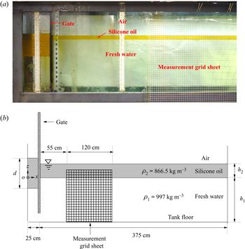
 $^{-3}$). To add the two fluids in the tank, first fresh water is added as the lower fluid. A polystyrene foam sheet, with mass density smaller than the fresh water, is used to reduce the disturbance when adding the silicone oil to the tank. The polystyrene foam is distributed uniformly over the fresh water and the silicone oil is added gradually through the foam sheet. The sheet is removed before the start of the experiments. Overall, using this approach, little to no mixing is observed. Figure 1(a) shows the physical wave tank and figure 1(b) shows the schematic of the wave tank. The top layer is open to the atmosphere.
Set-up of the experiments on internal solitary waves in a two-layer fluid system with a free surface. (a) The physical wave tank and (b) schematic of the wave tank. Figure not to scale.

To generate the internal solitary waves, the gravity collapse method (e.g. Kao et al. Reference Kao, Pan and Renouard1985) is used. Once the two fluid layers are filled and settled, a gate is placed at  $25$ cm away from the left wall of the tank. A prescribed volume of silicone oil with depth
 $d$ is added behind the gate; see figure 1.
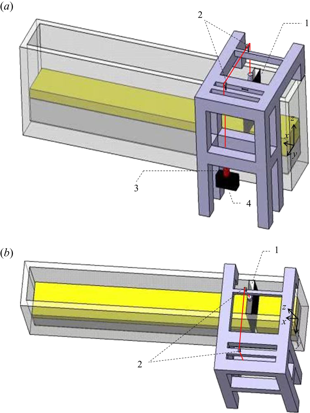
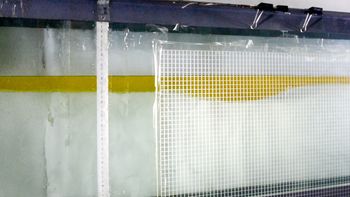
A pulley system is designed and used to remove the gate automatically and rapidly. One side of the pulley system is a weight that is connected by an electromagnetic relay, and the other side is the gate. Figure 2 shows the schematic of the pulley system. At the beginning of each test (corresponding to time  $t=0~\textrm {s}$), the power supply of the electromagnet relay is cut off. The weight then goes into free fall and it removes the gate quickly, resulting in the generation of a single solitary wave of depression form. The wave then propagates to the right in the main section of the tank. Figure 3 shows a snapshot of an internal solitary wave propagating in the tank.
Sketch of the pulley system, showing: 1, gate; 2, pulley; 3, electromagnetic relay; and 4, weight. (a) Side view and (b) plan view.

Snapshot of an internal solitary wave propagating in the tank at approximately  $t=4~\textrm {s}$ (the gate is removed completely at
 $t=0~\textrm {s}$).

2.2. Measurements
The internal solitary waves generated by the removal of the gate propagate along the interface of the two fluids to the right. Measurements focus on the internal-wave profile. A digital camera capable of recording videos at 60 frames per second is used. A transparent reference grid sheet,  $120$ cm long,
 $1~\text {cm} \times 1~\text {cm}$ size per grid, is fixed to the tank wall at
 $55$ cm away from the gate. The location of the transparent grid sheet is chosen such that it is far from the right boundary to avoid any reflections during the measurements. The vertical location of the grid sheet is chosen carefully to cover the entire wave. The digital camera is located right in front of the transparent grid sheet and level with the interface of the fluids and recorded the motion of the internal solitary wave.
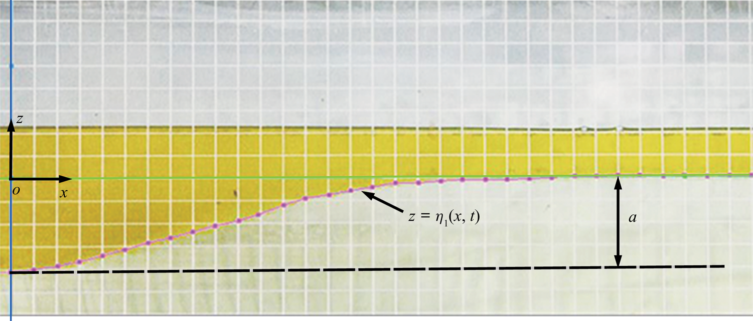
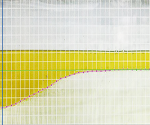
Recordings of the camera as the wave passed through the grid sheet are used to determine the wave profile. A sample recording of the internal solitary wave passing behind the sheet is shown in figure 4, where the  $ox$ axis is set at the undisturbed interface and the internal solitary-wave amplitude
 $a$ and profile
 $z=\eta _1(x,t)$ are shown. The GetData Graph Digitizer software is used to obtain the front half-profile of the internal solitary wave manually. Careful attention is given to read the profiles of all cases at about the same location across the grid sheet, when the wave is right in front of the lens. The measurement error is
 $\varepsilon \approx \pm 0.06$ cm along the vertical direction due to the resolution of the recording picture and the GetData Graph Digitizer software. Each test is conducted twice to assess the repeatability of the experiments.
A sample recording of the internal solitary wave behind the transparent sheet.

2.3. Experimental cases and the MCC-FS results
The upper and lower fluids (silicone oil and water, respectively) are kept the same in all laboratory experiments, resulting in the relative density ratio of  $\rho _2/\rho _1=0.869$. In all laboratory experiments, the depths of the lower and upper layers are fixed at
 $h_1 = 30$ cm and
 $h_2 = 2$ cm, respectively, corresponding to the depth ratio of
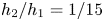 $h_2/h_1 = 1/15$. Three initial depths (volumes in three dimensions) of the silicone oil behind the gate are considered, namely
 $d = 8$ cm,
 $d = 10$ cm and
 $d = 12$ cm. As a result, we obtained internal solitary waves with amplitudes
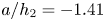 $a/h_2=-1.41$,
 $-1.91$ and
 $-2.35$. The parameters of the physical experiments are given in table 1.
Parameters and results of the physical experiments conducted at the internal wave flume of HEU.

It was found that, for a given collapse height, solitary waves generated by complete removal of the gate have larger amplitudes than those generated by partial removal of the gate. In either methods of partial or complete removal of the gate, solitary waves with the desired amplitudes can be generated by carefully adjusting the initial collapse height. We observed no differences between the profile of solitary waves of the same amplitude, whether generated by complete or partial removal of the gate. Internal solitary waves in this paper are generated by partial removal of the gate.
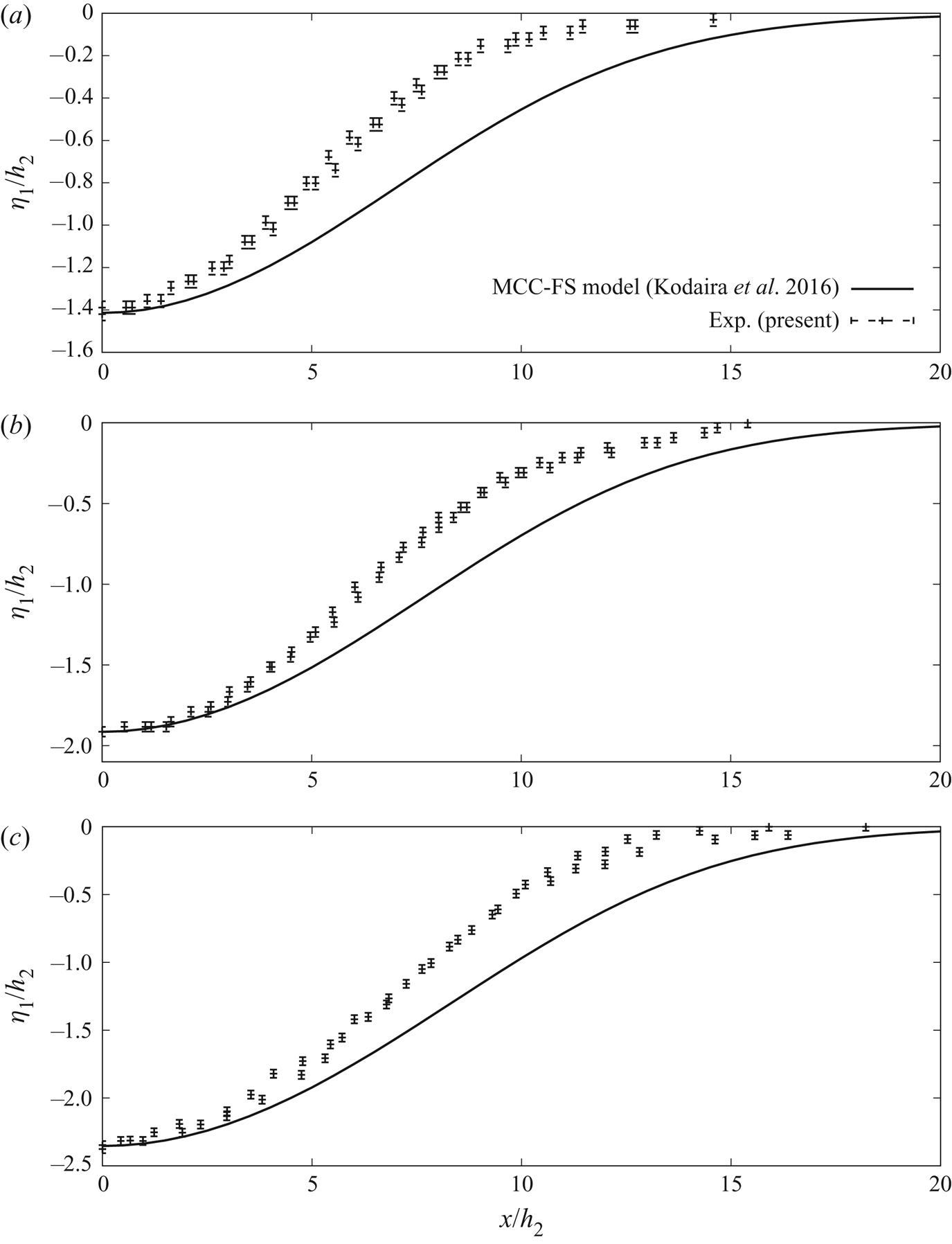
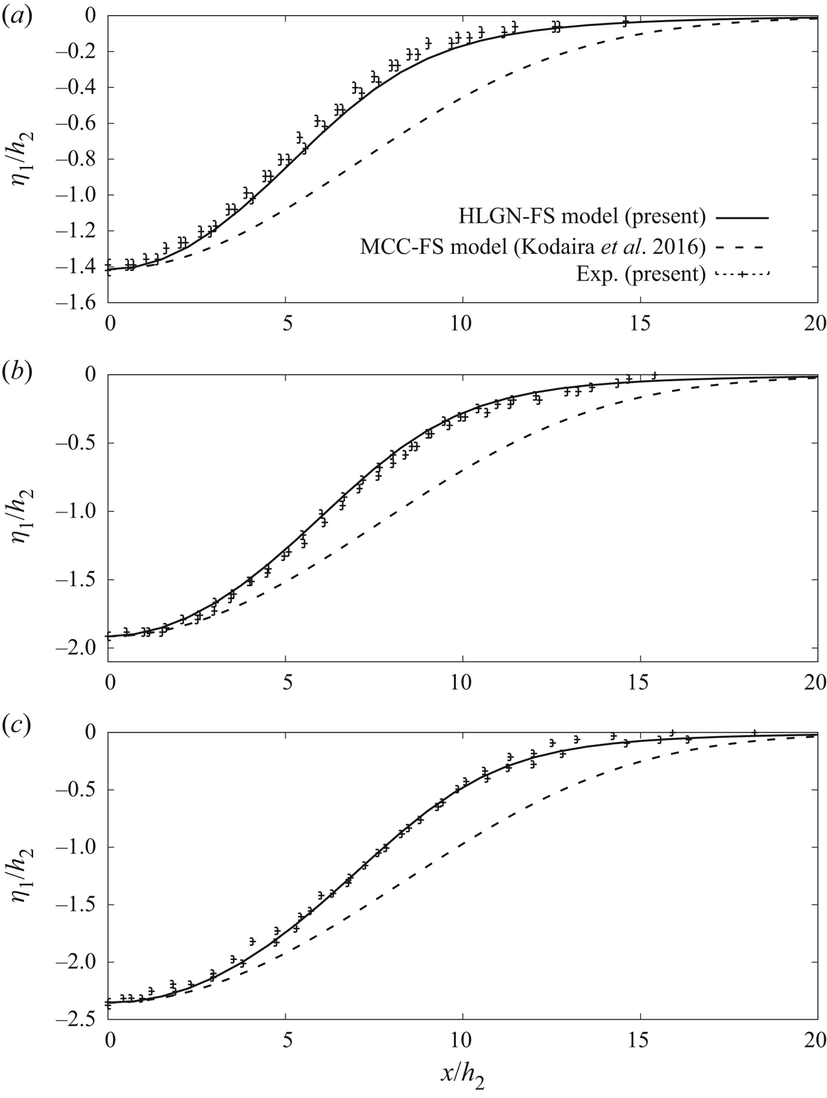
Results of the two repeats of the laboratory measurements are shown in figure 5. Also shown in the figure are the results of the MCC-FS model of Kodaira et al. (Reference Kodaira, Waseda, Miyata and Choi2016), included for comparison. We find that the physical experiments are repeatable. From the comparison, it is clear that the wave profiles obtained by the MCC-FS model are much wider than the physical experimental measurements. This is not surprising given that the case of 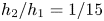 $h_{2}/h_{1}=1/15$ belongs to the deep configuration, and the MCC model is valid only for a shallow configuration (see Camassa et al. Reference Camassa, Choi, Michallet, Rusas and Sveen2006).
Profiles of internal solitary waves, for  $\rho _2/\rho _1=0.869$ and
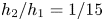 $h_2/h_1=1/15$: (a)
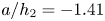 $a/h_2=-1.41$, (b)
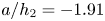 $a/h_2=-1.91$ and (c)
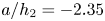 $a/h_2=-2.35$.

Hence, it is concluded that, for the present case of the density ratio  $\rho _2/\rho _1=0.869$ and depth ratio
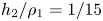 $h_2/\rho _1=1/15$, the MCC-FS model does not accurately describe the internal solitary waves with a free surface. Instead, a strongly nonlinear model for a deep configuration is required to solve such a problem accurately. The development of such a model is the objective of the next section.
3. Two-layer high-level Green–Naghdi model with free-surface effects
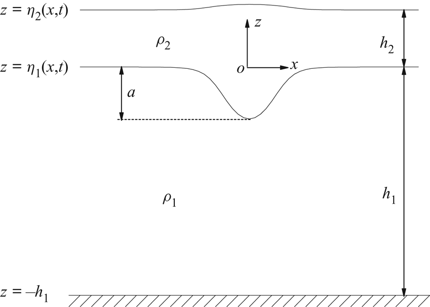
In this section, we will develop the two-layer HLGN-FS model. Here the two-dimensional model is considered, although this is not a requirement in general. The fluid is assumed to be inviscid and incompressible. The coordinate origin is set at the still interface surface;  $x$ is the horizontal axis, positive to the right, and
 $z$ is the vertical axis, positive up.
For both the upper layer and the lower layer, the continuity equation is written as
 \begin{equation} \frac{{\partial {u}}}{{\partial x}} + \frac{{\partial {w}}}{{\partial z}} = 0, \end{equation}
where  $u$ and
 $w$ are the velocity components in the
 $x$ and
 $z$ directions, respectively.
The Euler equations are written as
 \begin{gather} \frac{{\partial {u}}}{{\partial t}} + {u}\frac{{\partial {u}}}{{\partial x}} + {w}\frac{{\partial {u}}}{{\partial z}} = - \frac{1}{{{\rho}}}\frac{{\partial {p}}}{{\partial x}}, \end{gather}
 \begin{gather}\frac{{\partial {w}}}{{\partial t}} + {u}\frac{{\partial {w}}}{{\partial x}} + {w}\frac{{\partial {w}}}{{\partial z}} = - \frac{1}{{{\rho}}}\left( {\frac{{\partial {p}}}{{\partial z}} + {\rho}g} \right), \end{gather}
where  $t$ is the time,
 $\rho$ is the mass density of the fluid,
 $p$ is the pressure and
 $g$ is the gravitational acceleration.
In this paper, the free surface, interface and bottom boundary are expressed by  $z=\eta _{2}(x,t)$,
 $z=\eta _{1}(x,t)$ and
 $z=-h_{1}$, respectively, where
 $h_1$ is constant;
 $\rho _2$ is the mass density of the upper-layer fluid and
 $\rho _1$ is the mass density of the lower-layer fluid, also shown in figure 6.
Set-up of the theoretical tank of internal solitary-wave generation and propagation in a two-layer fluid system with a free surface.

The kinematic boundary conditions are expressed as
 \begin{gather} {w^U} = \frac{{\partial {\eta _2}}}{{\partial t}} + {u^U}\frac{{\partial {\eta _2}}}{{\partial x}}{,}\quad z=\eta_{2}(x,t), \end{gather}
 \begin{gather}{w^U} = \frac{{\partial {\eta _1}}}{{\partial t}} + {u^U}\frac{{\partial {\eta _1}}}{{\partial x}}{,}\quad z=\eta_{1}(x,t), \end{gather}
 \begin{gather}{w^L} = \frac{{\partial {\eta _1}}}{{\partial t}} + {u^L}\frac{{\partial {\eta _1}}}{{\partial x}}{,}\quad z=\eta_{1}(x,t), \end{gather}
 \begin{gather}{w^L} =0{,}\quad z=-h_1, \end{gather}
where the superscripts ‘U’ and ‘L’ indicate the variable in the upper layer and lower layer, respectively.
In the HLGN model (see e.g. Zhao et al. Reference Zhao, Ertekin, Duan and Webster2016), the velocity field is given as
 \begin{gather} u^{U}(x,z,t) = \sum_{n = 0}^{K^U} {{u^U_n}(x,t)z^{n}},\quad w^{U}(x,z,t) = \sum_{n = 0}^{K^U} {{w^U_n}(x,t)z^{n}}, \end{gather}
 \begin{gather}u^{L}(x,z,t) = \sum_{n = 0}^{K^L} {{u^L_n}(x,t)z^{n}},\quad w^{L}(x,z,t) = \sum_{n = 0}^{K^L} {{w^L_n}(x,t)z^{n}}, \end{gather}
where  $K^U$ is the level of the HLGN model applied for the upper layer and
 $K^L$ is the level of the HLGN model applied for the lower layer, respectively;
 $K^U$ and
 $K^L$ can be chosen independent of each other. We use HLGN-
 ${K^U}$-
 ${K^L}$ to indicate which level we use for each layer (in this paper, we select
 $K^U= K^L$ to obtain the converged HLGN results, but this is not necessary in general). In the above,
 $u^U_{n}$,
 $w^U_{n}$,
 $u^L_{n}$ and
 $w^L_{n}$ are the unknown velocity coefficients that are determined as part of the solution.
Substituting (3.4) into (3.1) results in the following relations:
 \begin{gather} u_{{K^U}}^U = 0, \end{gather}
 \begin{gather}w_n^U = - \frac{1}{n}\frac{{\partial u_{n - 1}^U}}{{\partial x}}{,}\quad n=1,2,\ldots,K^U, \end{gather}
 \begin{gather}u_{{K^L}}^L = 0, \end{gather}
 \begin{gather}w_n^L = - \frac{1}{n}\frac{{\partial u_{n - 1}^L}}{{\partial x}}{,}\quad n=1,2,\ldots,K^L. \end{gather}
Substituting (3.4) into (3.2), and multiplying each term by  $z^n$ and integrating from
 $\eta _1$ to
 $\eta _2$ for the upper layer, and from
 $-h_1$ to
 $\eta _1$ for the lower layer, will result in
 \begin{align} &\frac{\partial }{{\partial x}} {( }{G_n^U + gS1_n^U} {) }+ nE_{n - 1}^U - {\eta_{1} ^n}\frac{\partial }{{\partial x}} {( }{G_0^U + gS1_0^U} {) }\nonumber\\ &\quad + {( }{{\eta_{2} ^n} - {\eta_{1} ^n}} {) }\frac{\partial }{{\partial x}} \left( {\frac{{{{\hat p}^U}}}{{{\rho _2}}}} \right) = 0{, }\quad n=1,2,\ldots,K^U, \end{align}
 \begin{align} & \frac{\partial }{{\partial x}} {( }{G_n^L + gS1_n^L} {) }+ nE_{n - 1}^L - {(-h_1) ^n}\frac{\partial }{{\partial x}} {( }{G_0^L + gS1_0^L} {) }\nonumber\\ &\quad + {( }{{\eta_{1} ^n} - {(-h_1) ^n}} {) }\frac{\partial }{{\partial x}} \left( {\frac{{{{\hat p}^L}}}{{{\rho _1}}}} \right) = 0{, }\quad n=1,2,\ldots,K^L, \end{align}
where  ${\hat p}^U=0$ is the pressure at the upper surface of the upper layer (without loss of generality),
 ${\hat p}^L$ is the pressure at the upper surface of the lower layer, which equals the pressure at the lower surface of the upper layer
 ${\bar p}^U$, which is written as
 \begin{equation} {\hat p^L} = {\bar p^U} = {\rho _2}G_0^U + {\rho _2}gS1_0^U, \end{equation}
and
 \begin{gather} {E_n^U} = \sum_{m = 0}^{K^U} {\left( {\frac{{\partial {u_m^U}}}{{\partial t}}{S2_{mn}^U} + \frac{{\partial {u_m^U}}}{{\partial x}}{Q_{mn}^U} + {u_m^U}{H_{mn}^U}} \right)}, \end{gather}
 \begin{gather}{G_n^U} = \sum_{m = 0}^{K^U} {\left( {\frac{{\partial {w_m^U}}}{{\partial t}}{S2_{mn}^U} + \frac{{\partial {w_m^U}}}{{\partial x}}{Q_{mn}^U} + {w_m^U}{H_{mn}^U}} \right)}, \end{gather}
 \begin{gather}{Q_{mn}^U} = \sum_{r = 0}^{K^U} {{u_r^U}{S3_{mrn}^U}},\quad {H_{mn}^U} = \sum_{r = 0}^{K^U} {{w_r^U}S4_{mrn}^U}, \end{gather}
 \begin{gather}S1_n^U = \int_{\eta_{1}} ^{\eta_{2}} {z^n\, \textrm{d} z},\quad S2_{mn}^U = \int_{\eta_{1}} ^{\eta_{2}} {z^{m + n}\, \textrm{d} z}, \end{gather}
 \begin{gather}S3_{mrn}^U = \int_{\eta_{1}} ^{\eta_{2}} {z^{m + r + n}\, \textrm{d} z},\quad S4_{mrn}^U = m\int_{\eta_{1}} ^{\eta_{2}} {z^{m + r + n - 1}\, \textrm{d} z}. \end{gather}
We note that the expression for the lower layer is obtained by changing ‘U’ to ’L’,  $\eta _{1}$ to
 $-h_1$, and
 $\eta _{2}$ to
 $\eta _{1}$ in (3.8).
Substituting (3.4) into (3.3), we obtain
 \begin{gather} \frac{{\partial \eta_{2} }}{{\partial t}} = \sum_{n = 0}^{{K^U}} \,{\eta_{2} ^n}\left( {w_n^U - \frac{{\partial \eta_{2} }}{{\partial x}}u_n^U} \right), \end{gather}
 \begin{gather}w_0^U = \frac{{\partial {\eta _1}}}{{\partial t}} + \frac{{\partial {\eta _1}}}{{\partial x}}u_0^U + \sum_{n = 1}^{{K^U}} {\eta _1^n\left( {\frac{1}{n}\frac{{\partial u_{n - 1}^U}}{{\partial x}} + \frac{{\partial {\eta _1}}}{{\partial x}}u_n^U} \right)}, \end{gather}
 \begin{gather}\frac{{\partial \eta_{1} }}{{\partial t}} = \sum_{n = 0}^{{K^L}} \,{\eta_{1} ^n}\left( {w_n^L - \frac{{\partial \eta_{1} }}{{\partial x}}u_n^L} \right), \end{gather}
 \begin{gather}w_0^L = \sum_{n = 1}^{{K^L}} {\frac{{{{\left( { - {h_1}} \right)}^n}}}{n}\frac{{\partial u_{n - 1}^L}}{{\partial x}}}. \end{gather}
There is no gap at the interface between the two fluids at any time by assumption. Hence, the solutions of the two layers are coupled at the interface. Therefore, we can eliminate  $w^U_n$ and
 $w^L_n$ by using (3.5b), (3.5d), (3.9b) and (3.9d). As a result, the unknowns are
 $\eta _2$,
 $\eta _1$,
 $u^U_n\ (n=0,1,\ldots ,K^U-1)$ and
 $u^L_n\ (n=0,1,\ldots ,K^L-1)$. The number of unknowns is
 $K^U+K^L+2$. On the other hand, the number of equations, including (3.6), (3.9a) and (3.9c), is also
 $K^U+K^L+2$. Hence, the problem is closed.
4. Solution algorithm
In the HLGN-FS equations, (3.6) is expressed by
 \begin{equation} {\boldsymbol{\mathsf{A}}}\dot{\xi}_{,xx}+{\boldsymbol{\mathsf{B}}}\dot{\xi}_{,x}+ {\boldsymbol{\mathsf{C}}}\dot{\xi}=\textbf{f}, \end{equation}
where  ${\boldsymbol{\mathsf{A}}}$,
 ${\boldsymbol{\mathsf{B}}}$ and
 ${\boldsymbol{\mathsf{C}}}$ are
 $(K^{U}+K^{L}) \times (K^{U}+K^{L})$ matrices,
 $\textbf {f}$ is a (
 $K^{U}+K^{L}$) vector and
 \begin{equation} \dot{\xi}(x,t)=[\dot{u}^{U}_{0}, \ \dot{u}^{U}_{1}, \ldots, \dot{u}^{U}_{K^{U}-1}, \ \dot{u}^{L}_{0}, \ \dot{u}^{L}_{1}, \ldots, \dot{u}^{L}_{K^{L}-1}]^\textrm{T}. \end{equation}
The dot over a variable indicates time derivative, i.e.  $\dot {\xi }=\partial {\xi }/\partial {t}$; the subscript after a comma is differentiation with respect to the indicated variable; and
 ${\boldsymbol{\mathsf{A}}}$,
 ${\boldsymbol{\mathsf{B}}}$,
 ${\boldsymbol{\mathsf{C}}}$ and
 $\textbf {f}$ are functions of
 $\eta _{1}(x,t)$,
 $\eta _{2}(x,t)$,
 $\xi (x,t)$ and their spatial derivatives. For simplification, this dependence will not be shown here.
The above system of differential equations is solved by use of the spatial finite difference discretization. The domain of  $x$ over which a solution to the equations is desired is assumed to have a uniform grid of
 $x$ values, spaced a distance of
 ${\rm \Delta} {x}$ apart. The
 $i$th point on the grid is denoted by
 ${x_i} = i{\rm \Delta} {x}$ for
 $i = 1, 2, \ldots , nx$. Time is discretized with intervals
 ${\rm \Delta} {t}$, with
 ${t_j} = j{\rm \Delta} {t}$. The value of the solution vector
 $\xi ({x_i},{t_j})$ will be denoted by
 ${{\xi } ^{(i)}}$ (
 $\,j$ is omitted in the following part, because we refer to the same
 $j$ time) and similar superscripts will be used for other vectors and matrices. The spatial derivatives
 ${\dot {\xi } _{,x}}$ and
 ${\dot {\xi } _{,xx}}$ are approximated by the five-point central difference scheme as
 \begin{gather} \dot {{\xi}}_{,x}^{(i)} = {\frac{1}{12{\rm \Delta} x}}({\dot {{\xi}} ^{(i - 2)}} - 8{\dot {{\xi}} ^{(i - 1)}} + 8{\dot {{\xi}} ^{(i + 1)}} - {\dot {{\xi}}^{(i + 2)}}), \end{gather}
 \begin{gather}\dot {{\xi}}_{,xx}^{(i)} = {\frac{1}{12{\rm \Delta} {x^2}}}( - {\dot {{\xi}}^{(i - 2)}} + 16{\dot {{\xi}} ^{(i - 1)}} - 30{\dot {{\xi}} ^{(i)}} + 16{\dot {{\xi}} ^{(i + 1)}} - {\dot {{\xi}} ^{(i + 2)}}). \end{gather}
The five-point central difference scheme provides fourth-order accuracy for the first and second derivatives, and second-order accuracy for the third derivative. With these approximations, (4.1) can now be written as
 \begin{equation} \tilde{{\boldsymbol{\mathsf{A}}}}^{(i)}{\dot {{\zeta}}^{(i - 2)}} + \tilde{{\boldsymbol{\mathsf{B}}}}^{(i)}{\dot {{\zeta}}^{(i - 1)}} + \tilde{{\boldsymbol{\mathsf{C}}}}^{(i)}{\dot {{\zeta}}^{(i)}} + \tilde{{\boldsymbol{\mathsf{D}}}}^{(i)}{\dot {{\zeta}}^{(i + 1)}} + \tilde{{\boldsymbol{\mathsf{E}}}}^{(i)}{\dot {{\zeta}}^{(i + 2)}}={{\textbf{f}}}^{(i)}, \end{equation}
where
 \begin{gather} \tilde{{\boldsymbol{\mathsf{A}}}}^{(i)} = - {{{\boldsymbol{\mathsf{A}}}}^{(i)}}{\frac{1}{{12{\rm \Delta} {x^2}}} }+ {{{\boldsymbol{\mathsf{B}}}}^{(i)}}{\frac{1}{{12{\rm \Delta} x}}}, \end{gather}
 \begin{gather}\tilde{{\boldsymbol{\mathsf{B}}}}^{(i)} = {{{\boldsymbol{\mathsf{A}}}}^{(i)}}{\frac{{16}}{{12{\rm \Delta} {x^2}}} }- {{{\boldsymbol{\mathsf{B}}}}^{(i)}}{\frac{8}{{12{\rm \Delta} x}}}, \end{gather}
 \begin{gather}\tilde{{\boldsymbol{\mathsf{C}}}}^{(i)} = - {{{\boldsymbol{\mathsf{A}}}}^{(i)}}{\frac{{30}}{{12{\rm \Delta} {x^2}}} }+ {{{\boldsymbol{\mathsf{C}}}}^{(i)}}, \end{gather}
 \begin{gather}\tilde{{\boldsymbol{\mathsf{D}}}}^{(i)} = {{{\boldsymbol{\mathsf{A}}}}^{(i)}}{\frac{{16}}{{12{\rm \Delta} {x^2}}} }+ {{\boldsymbol{\mathsf{B}}}^{(i)}}{\frac{8}{{12{\rm \Delta} x}}}, \end{gather}
 \begin{gather}\tilde{{\boldsymbol{\mathsf{E}}}}^{(i)} = - { {{\boldsymbol{\mathsf{A}}}}}^{(i)}{\frac{1}{{12{\rm \Delta} {x^2}}} }-{ {{\boldsymbol{\mathsf{B}}}}}^{(i)}{\frac{1}{{12{\rm \Delta} x}}}. \end{gather}
The algorithm to solve (4.4) can be found in Zhao, Duan & Ertekin (Reference Zhao, Duan and Ertekin2014). The algorithm obtains the values of  ${{\dot u}^{U}_0}, {{\dot u}^{U}_1}, \ldots , {{\dot u}^{U}_{K^U-1}}, {{\dot u}^{L}_0}, {{\dot u}^{L}_1}, \ldots , {{\dot u}^{L}_{K^L-1}}.$ In addition,
 $\dot \eta _{1}(x,t)$ and
 $\dot \eta _{2}(x,t)$ can be calculated by means of (3.9a) and (3.9c). We then use the fourth-order Adams predictor–corrector scheme for time marching.
The initial values are given by the steady solution of the internal solitary waves with a free surface provided by the HLGN-FS model. For a similar method to obtain the steady solution, see Zhao et al. (Reference Zhao, Ertekin, Duan and Webster2016) for details.
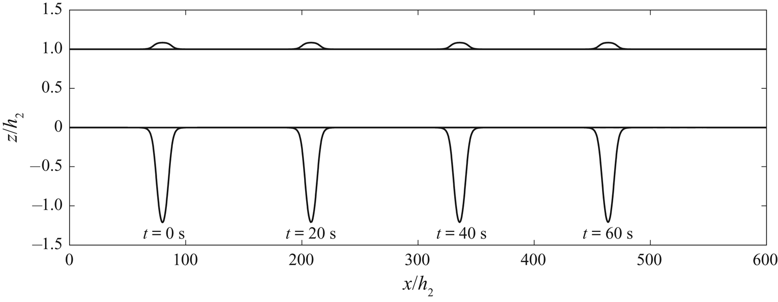
As an example, we show an internal solitary wave propagating at different times in figure 7. The parameters are  $\rho _2/\rho _1=0.859$,
 $h_2/h_1=1/5$ and
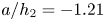 $a/h_2=-1.21$. From
 $t=0$ to
 $t=60\ \textrm {s}$, we find that the internal solitary wave propagates steadily. Meanwhile, since we use the pressure continuity condition at the interface given in (3.7) (rather than velocity continuity), a velocity jump across the interface is allowed. This, however, does not have any effect on the numerical simulation. Numerical instability was observed for the MCC-RL model, shown by Jo & Choi (Reference Jo and Choi2008).
Snapshots of the theoretical internal solitary wave with a free surface at different times,  $\rho _2/\rho _1=0.859$,
 $h_2/h_1=1/5$ and
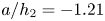 $a/h_2=-1.21$.

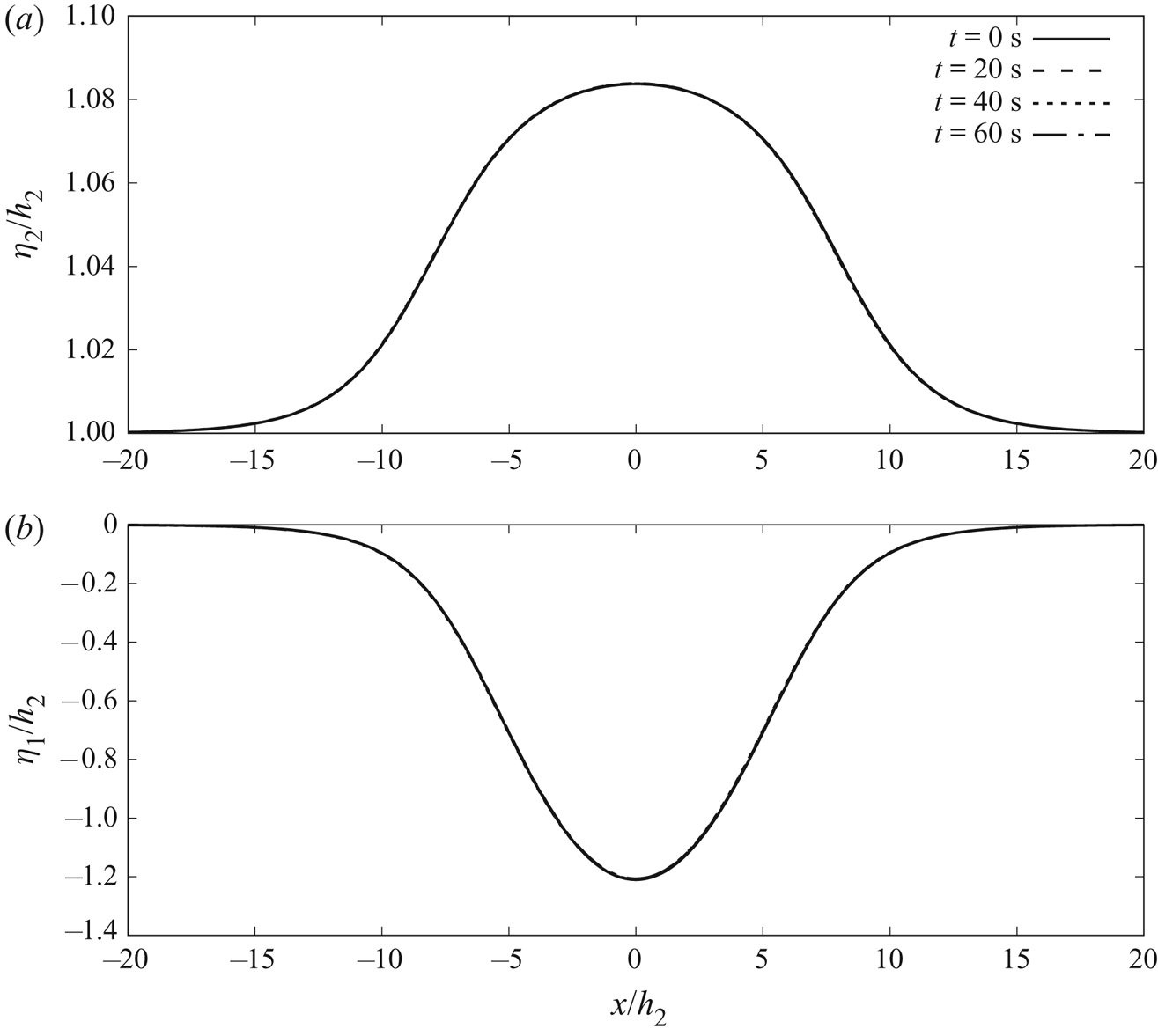
For comparison, in figure 8 we plot the internal solitary wave (figure 8b) and the free-surface elevation (figure 8a) of different times on top of each other. We observe that at  $t=0\ \text {s}, 20\ \text {s}, 40\ \text {s}$ and
 $60\ \text {s}$, the wave profiles show very good agreement. Thus, we have obtained an accurate solution of the internal solitary waves with a free surface.
Profiles of the internal solitary wave with a free surface at different times,  $\rho _2/\rho _1=0.859$,
 $h_2/h_1=1/5$ and
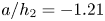 $a/h_2=-1.21$. (a) Profiles of the waves on the free surface (lines are on top of each other) and (b) profiles of internal solitary waves (lines are on top of each other).

5. Results and discussion
In this section, three numerical cases are considered as shown in table 2 and the solutions of internal solitary waves obtained by the HLGN-FS model are presented, including the wave profile, velocity field and wave speed. We note that, for each case, we have performed the HLGN-FS self-convergence tests by using different  $K^U$ and
 $K^L$ given in (3.4). We refer the reader to Zhao et al. (Reference Zhao, Duan and Ertekin2014) and Zhao et al. (Reference Zhao, Ertekin, Duan and Webster2016) for details of the HLGN convergence tests. The results presented in this paper are the converged HLGN-FS results, which can be regarded as Euler's solution that includes the free-surface effects.
Parameters of the numerical cases, and the laboratory experiments used for comparisons.

5.1. The case  $\rho _2/\rho _1=0.977$ and $h_2/h_1=1/4.13$


Grue et al. (Reference Grue, Jensen, Rusas and Sveen1999) conducted experiments on internal waves in a two-layer fluid system with a free surface. The rigid lid was set up on the free surface in their numerical simulations. Following the experiments of Grue et al. (Reference Grue, Jensen, Rusas and Sveen1999), we select the parameters as  $h_1 =0.62$ m,
 $h_2 =0.15$ m,
 $\rho _1 =1022~\text {kg~m}^{-3}$ and
 $\rho _2 =999~\text {kg~m}^{-3}$.
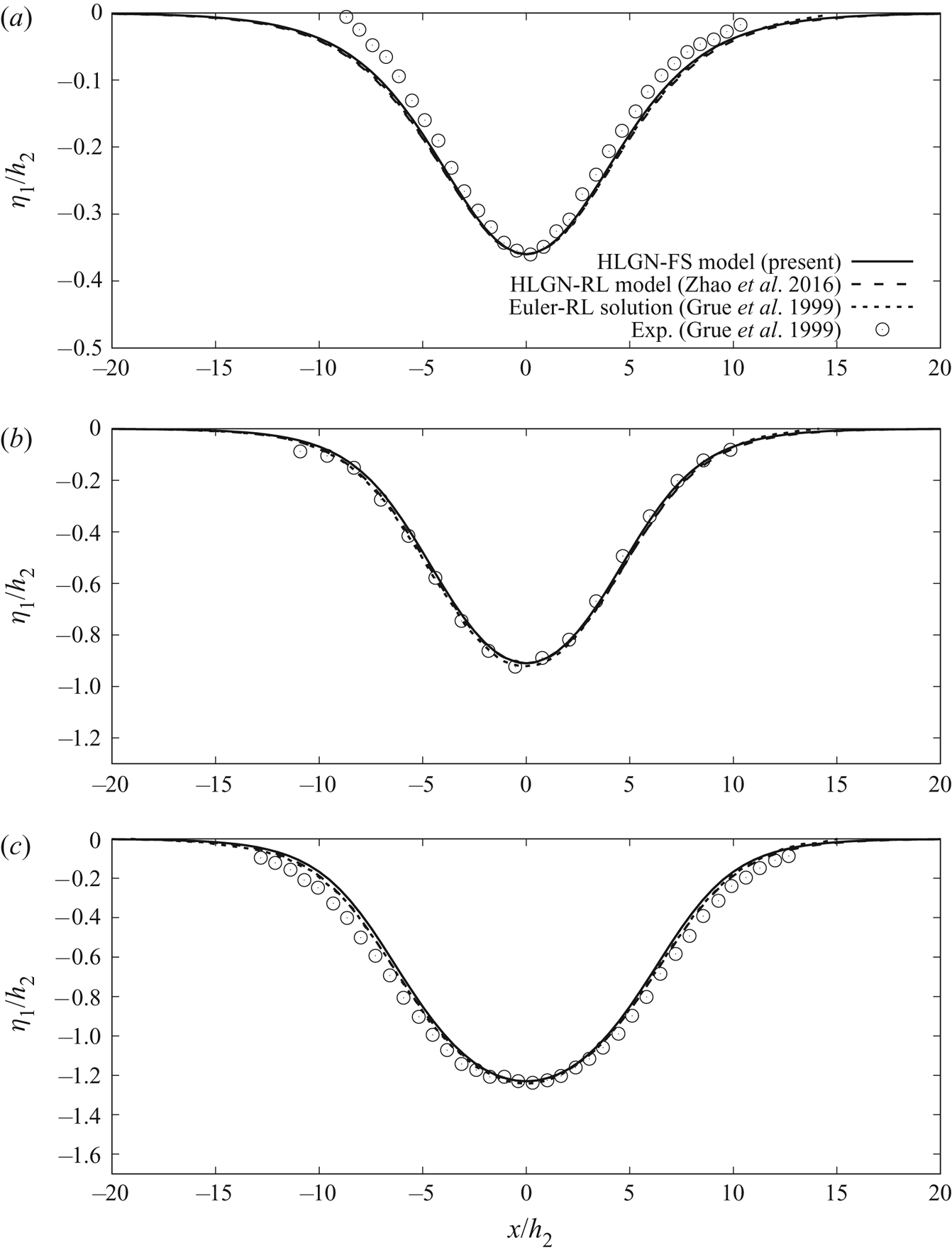
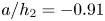
Three different amplitudes are considered here; they are  $a/{h_2}=-0.36$,
 $-0.91$ and
 $-1.23$. We compare the converged results of the HLGN-FS model (HLGN-3-3-FS results for this case) with the results of the HLGN-RL model of Zhao et al. (Reference Zhao, Ertekin, Duan and Webster2016) and the experimental data of Grue et al. (Reference Grue, Jensen, Rusas and Sveen1999) as shown in figure 9.
Profiles of internal solitary waves,  $\rho _2/\rho _1=0.977$,
 $h_2/h_1=1/4.13$ and (a)
 $a/h_2=-0.36$, (b)
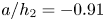 $a/h_2=-0.91$ and (c)
 $a/h_2=-1.23$.

From figure 9, we observe that the HLGN-FS results and the HLGN-RL results show very good agreement: both match the Euler-RL solution and experimental data well, even for the strongly nonlinear cases.
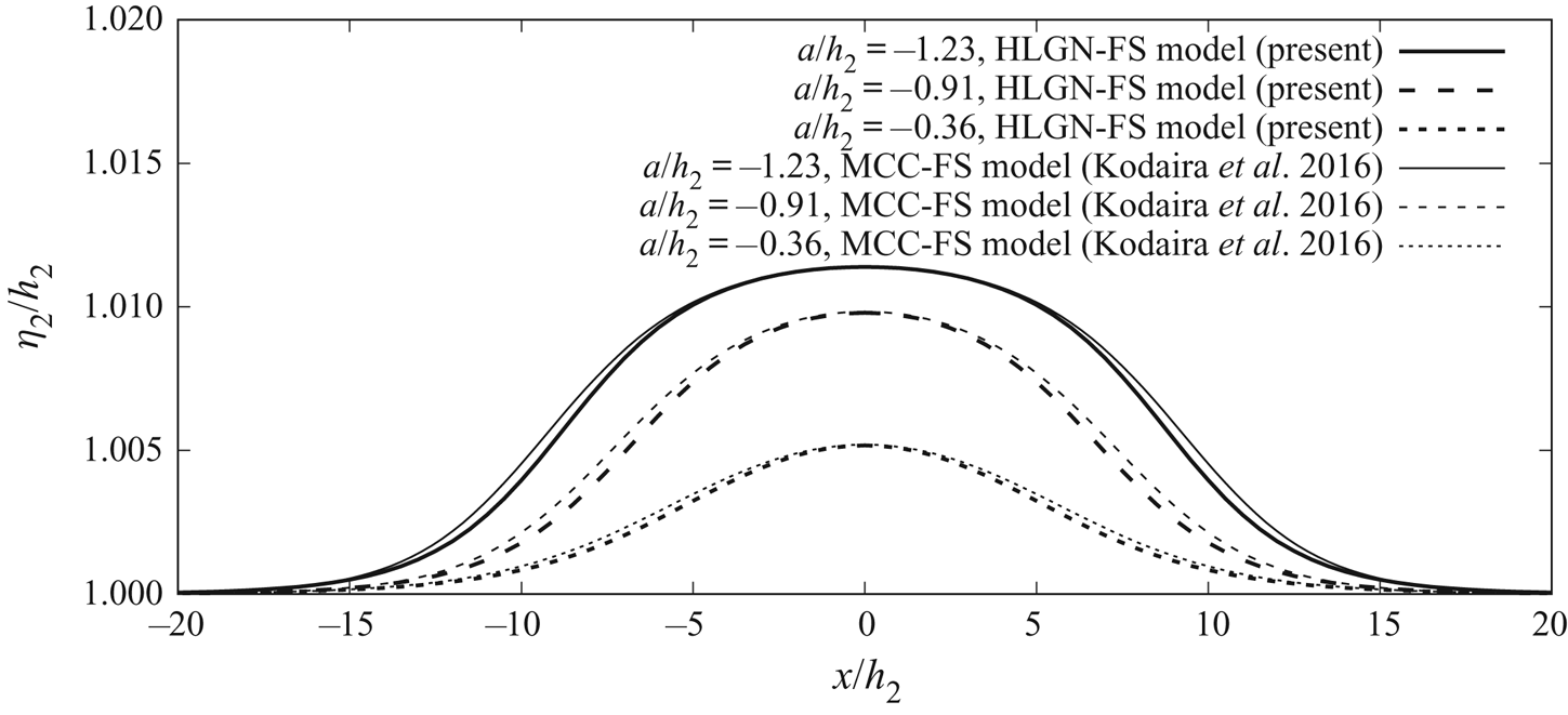
We next show the wave profiles on the free surface obtained by the HLGN-FS model and the MCC-FS model in figure 10. From figure 10, we find that a surface elevation exists at the free surface in each case. For the cases of internal solitary waves of  $a/h_2=-0.36, -0.91$ and
 $-1.23$, the amplitudes,
 $b$, of the surface waves are
 $b/h_2=0.5\,\%$,
 $1.0\,\%$ and
 $1.1\,\%$, respectively. Thus, it is demonstrated here that the disturbance on the free surface is quite small for the cases of Grue et al. (Reference Grue, Jensen, Rusas and Sveen1999). Meanwhile, we observe that the amplitudes of the surface wave predicted by the MCC-FS model show good agreement with the HLGN-FS model, while the wave profiles are slightly wider for the MCC-FS model than those of the HLGN-FS model.
Free-surface profiles,  $\rho _2/\rho _1=0.977$ and
 $h_2/h_1=1/4.13$.

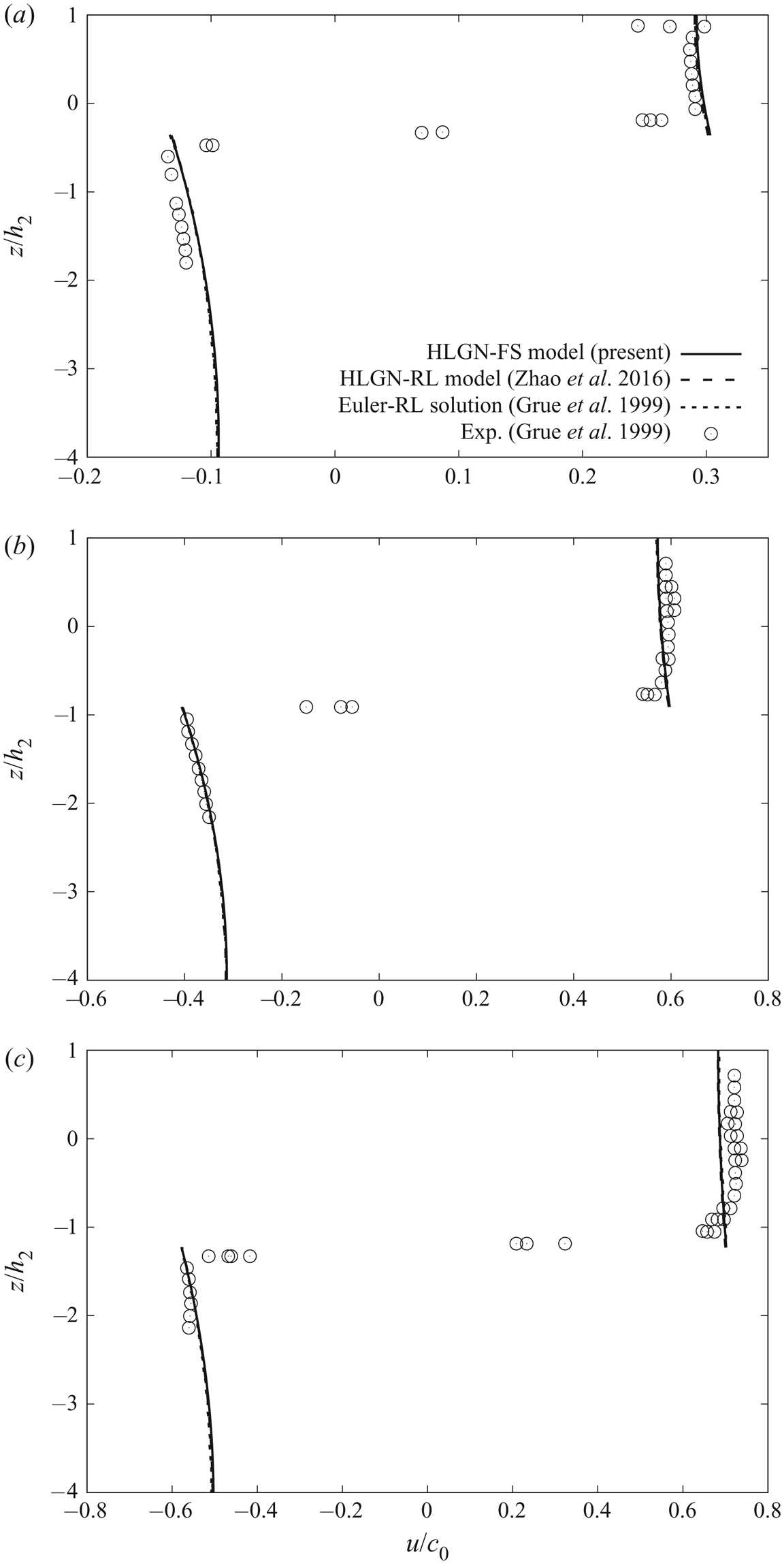
Next, we focus on the horizontal velocity along the fluid column at the maximal displacement. The results of the HLGN-FS model and the results of the HLGN-RL model are shown in figure 11, where the reference speed  $c_0=\sqrt {{g{h_1}{h_2}({\rho _1-\rho _2})}/{(\rho _2{h_1}+\rho _1{h_2})}}$ is the linear long-wave speed. We find that the horizontal velocity predicted by the HLGN-FS model shows good agreement with that predicted by the HLGN-RL model. They both match the Euler-RL solution of Grue et al. (Reference Grue, Jensen, Rusas and Sveen1999) and experimental data very well, as shown in figure 11.
Horizontal velocity along the fluid column at maximal displacement,  $\rho _2/\rho _1=0.977$,
 $h_2/h_1=1/4.13$ and (a)
 $a/h_2=-0.36$, (b)
 $a/h_2=-0.91$ and (c)
 $a/h_2= -1.23$.

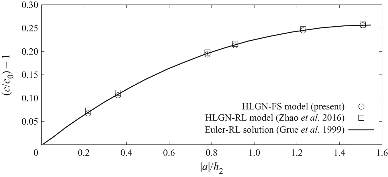
The relationship between the internal solitary-wave amplitude  $|a|/h_2$ and excess wave speed
 $c/c_0-1$ obtained by the HLGN-FS model and HLGN-RL model is shown in figure 12.
Excess propagation speed  $(c/c_0)-1$ versus amplitude,
 $\rho _2/\rho _1=0.977$ and
 $h_2/h_1=1/4.13$.

Figure 12 shows that the results of the HLGN-FS model are close to the HLGN-RL results and the Euler-RL solution of Grue et al. (Reference Grue, Jensen, Rusas and Sveen1999).
In general, in the cases with  $\rho _2/\rho _1=0.977$ and
 $h_2/h_1=1/4.13$, the results predicted by the HLGN-FS model and the HLGN-RL model agree very well with each other. This is because the mass densities between the upper-fluid layer and lower-fluid layer are very close to each other, and hence the free-surface disturbance is very small. Thus, it can be regarded as a rigid lid. This conclusion has been discussed previously, see e.g. Lamb (Reference Lamb1932) and Kodaira et al. (Reference Kodaira, Waseda, Miyata and Choi2016).
5.2. The case $\rho _2/\rho _1=0.859$ and $h_2/h_1=1/5$


Kodaira et al. (Reference Kodaira, Waseda, Miyata and Choi2016) conducted experiments on internal waves in a two-layer fluid system. The mass densities of the lower-fluid layer and the upper-fluid layer are  $\rho _1 =996~\text {kg~m}^{-3}$ and
 $\rho _2 =856~\text {kg~m}^{-3}$, respectively. The depths are
 $h_1 =0.25$ m and
 $h_2 =0.05$ m, respectively. The gravity collapse method was used to generate internal solitary waves in the experiments. By adjusting the interface displacement behind the gate, five internal solitary waves with different amplitudes were generated:
 $a/h_2=-0.24$,
 $-0.50$,
 $-0.77$,
 $-0.99$ and
 $-1.21$. In the numerical study of Kodaira et al. (Reference Kodaira, Waseda, Miyata and Choi2016), the MCC-RL model and the MCC-FS model were used to obtain the wave profiles and wave speed.
For simplification, we will show the results for three cases, namely the internal solitary waves with  $a/h_2=-0.50$,
 $-0.77$ and
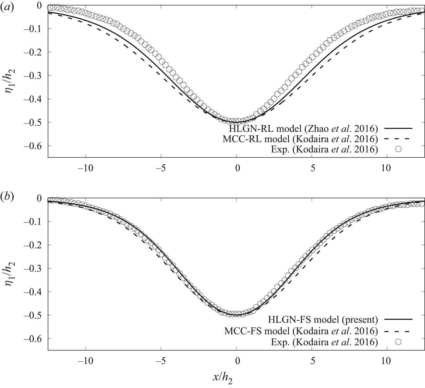
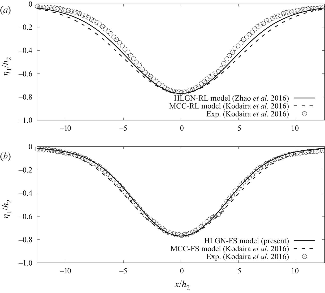
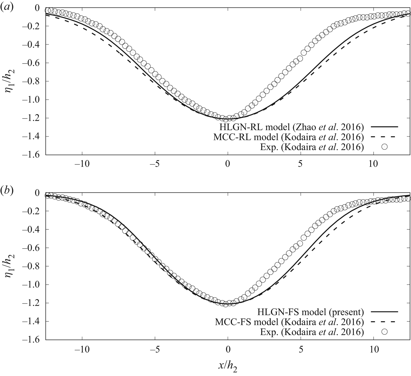
 $-1.21$. The wave profiles obtained by the HLGN-RL model and the HLGN-FS model are shown in figures 13–15, where the MCC-RL results and the MCC-FS results are also shown for comparison. The results provided by the models that are based on the rigid-lid assumption are not as accurate since the wave profiles they predict are wider than the experimental data; see figures 13(a), 14(a) and 15(a). When we consider the free-surface effects, we find that both the converged HLGN-FS results (HLGN-3-3 results for this case) and the MCC-FS results show very good agreement with the experimental data; see figures 13(b), 14(b) and 15(b). Thus, the effects of the free surface are important in these cases.
Profiles of internal solitary waves with  $a/h_2=-0.50$,
 $\rho _2/\rho _1=0.859$ and
 $h_2/h_1=1/5$. (a) Rigid-lid assumption and (b) with a free surface.

Profiles of internal solitary waves with  $a/h_2=-0.77$,
 $\rho _2/\rho _1=0.859$ and
 $h_2/h_1=1/5$. (a) Rigid-lid assumption and (b) with a free surface.

Profiles of internal solitary waves with 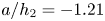 $a/h_2=-1.21$,
 $\rho _2/\rho _1=0.859$ and
 $h_2/h_1=1/5$. (a) Rigid-lid assumption and (b) with a free surface.

Comparisons between the numerical results and the experimental data are not so good for the largest wave amplitude, 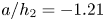 $a/h_2=-1.21$ shown in figure 15 for
 $x/h_2>0$. This is similar to the case of an internal solitary wave of
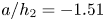 $a/h_2=-1.51$ in the experiments conducted by Grue et al. (Reference Grue, Jensen, Rusas and Sveen1999). Kodaira et al. (Reference Kodaira, Waseda, Miyata and Choi2016) pointed out that this large internal solitary wave suffered from the Kelvin–Helmholtz instability excited by the large shear across the interface.
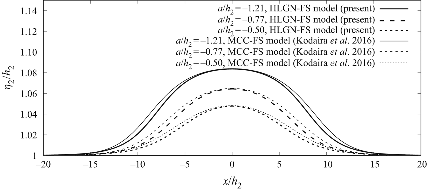
The wave profiles on the free surface obtained by the MCC-FS model and the HLGN-FS model for the cases of Kodaira et al. (Reference Kodaira, Waseda, Miyata and Choi2016) are shown in figure 16. It is determined that, for the cases of internal solitary waves for  $a/h_2=-0.50$,
 $-0.77$ and
 $-1.21$, the wave amplitudes on the free surface are
 $b/h_2=4.8\,\%$,
 $6.4\,\%$ and
 $8.4\,\%$. Thus, there are obvious disturbances on the free surface, and therefore it could not be regarded as a rigid lid. Again, we find that the MCC-FS model and the HLGN-FS model predict the same amplitude of the surface wave. The profiles obtained by the MCC-FS model are wider than these obtained by the HLGN-FS model.
Free-surface profiles, 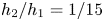 $\rho_2/\rho_1=0.859$ and $h_2/h_1=1/5$.

The velocity distribution along the fluid column at the maximal displacement for the three cases determined by the HLGN-FS model are shown in figure 17. We also apply the modified velocity expression given by Camassa et al. (Reference Camassa, Choi, Michallet, Rusas and Sveen2006) for the MCC-FS model and obtain the velocity distribution shown in figure 17 for comparison purposes. The MCC-FS results and the HLGN-FS results match very well.
Horizontal velocity along the fluid column at the maximal displacement,  $\rho _2/\rho _1=0.859$,
 $h_2/h_1=1/5$ and (a)
 $a/h_2=-0.50$, (b)
 $a/h_2=-0.77$ and (c)
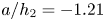 $a/h_2=-1.21$.

The relationship between the amplitude  $|a|/h_2$ and the excess wave speed
 $c/c_0-1$ obtained by the HLGN-FS model and the MCC-FS model is shown in figure 18. From figure 18, it is found that the two models are in good agreement in general.
Excess propagation speed  $(c/c_0)-1$ versus amplitude,
 $\rho _2/\rho _1=0.859$ and
 $h_2/h_1=1/5$.

In this case, we find that, when the density ratio between the two fluids is not close to  $1$ (e.g.
 $\rho _2/\rho _1=0.859$), the rigid-lid assumption does not provide an accurate description of the internal solitary waves. Instead, the models that include the free-surface effects should be applied. The MCC-FS model and the HLGN-FS model both describe the strongly nonlinear internal solitary waves with a free surface for the shallow configuration accurately.
5.3. The case $\rho _2/\rho _1=0.869$ and $h_2/h_1=1/15$

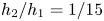
Next, we study a case where the depth ratio  $h_2/h_1$ is significantly smaller than other cases. Here, we consider the case of
 $\rho _2/\rho _1=0.869$ and
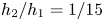
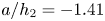
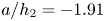
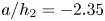
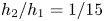 $h_2/h_1=1/15$. This is the same case as used in our laboratory experiments; see table 1 for the parameters. Here, we use the HLGN-FS model to calculate the strongly nonlinear internal solitary waves for this deep-configuration case. The internal solitary-wave profiles of this case are shown in figure 19. We also use the MCC-FS model in this case for comparison purposes. After carrying out the self-convergence test of the HLGN-FS model, it is determined that the HLGN-5-5-FS model can provide converged HLGN-FS results. We find that the converged HLGN-FS results match the experimental data very well. However, the MCC-FS results show large errors compared with the experimental data.
Profiles of internal solitary waves,  $\rho _2/\rho _1=0.869$,
 $h_2/h_1=1/15$ and (a)
 $a/h_2=-1.41$, (b)
 $a/h_2=-1.91$ and (c)
 $a/h_2=-2.35$.

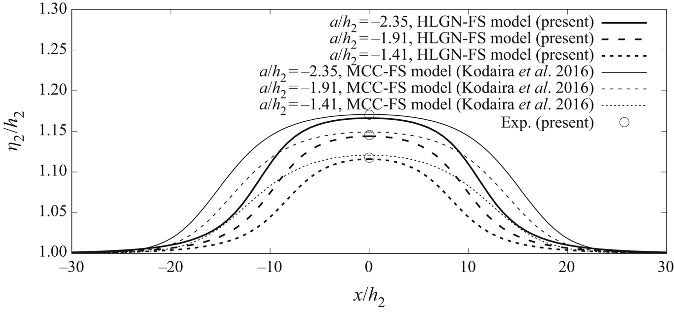
We then use the MCC-FS model and the HLGN-FS model to obtain the wave profiles on the free surface. Results are shown in figure 20. We find that, for the cases of 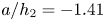 $a/h_2=-1.41$,
 $-1.91$ and
 $-2.35$, the wave amplitudes on the free surface are
 $b/h_2=11.6\,\%$,
 $14.4\,\%$ and
 $16.6\,\%$ obtained by the HLGN-FS model. Meanwhile, for this deep-configuration case, we find that the surface-wave profiles obtained by the MCC-FS model are obviously higher and wider than those obtained by the HLGN-FS model. Similar to La Forgia & Sciortino (Reference La Forgia and Sciortino2019), we measured the maximum surface elevation of the top-fluid layer recorded in the laboratory experiments as shown in figure 20. Good agreement is found between the numerical results and the experimental data.
Free-surface profiles, $\rho_2/\rho_1=0.869$ and $h_2/h_1=1/15$.

We note that, in the experiments of Kodaira et al. (Reference Kodaira, Waseda, Miyata and Choi2016), surface disturbance is observed towards the front of the internal solitary wave, and not over the trough. This surface disturbance is not observed in the present experiments. Further investigation is required to assess the existence of these surface disturbances.
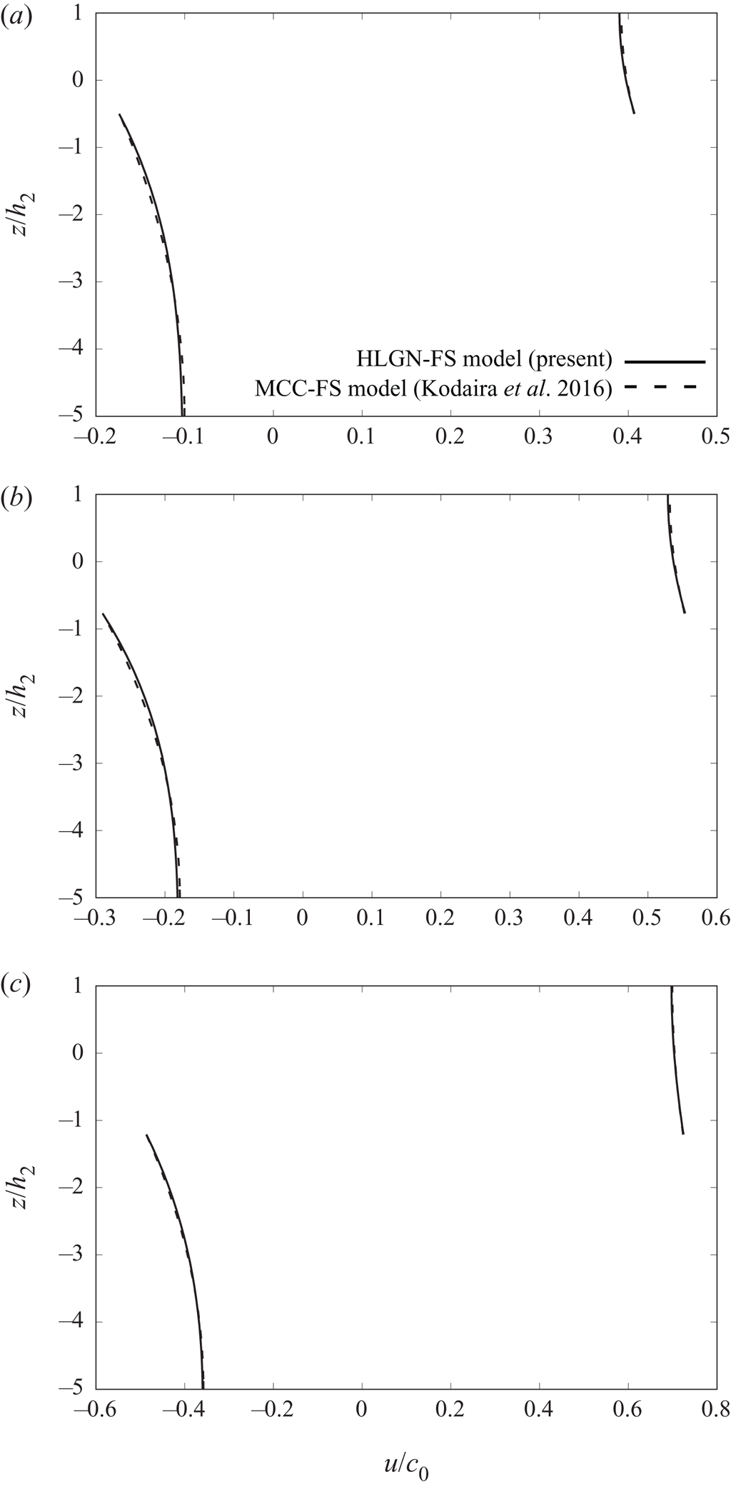
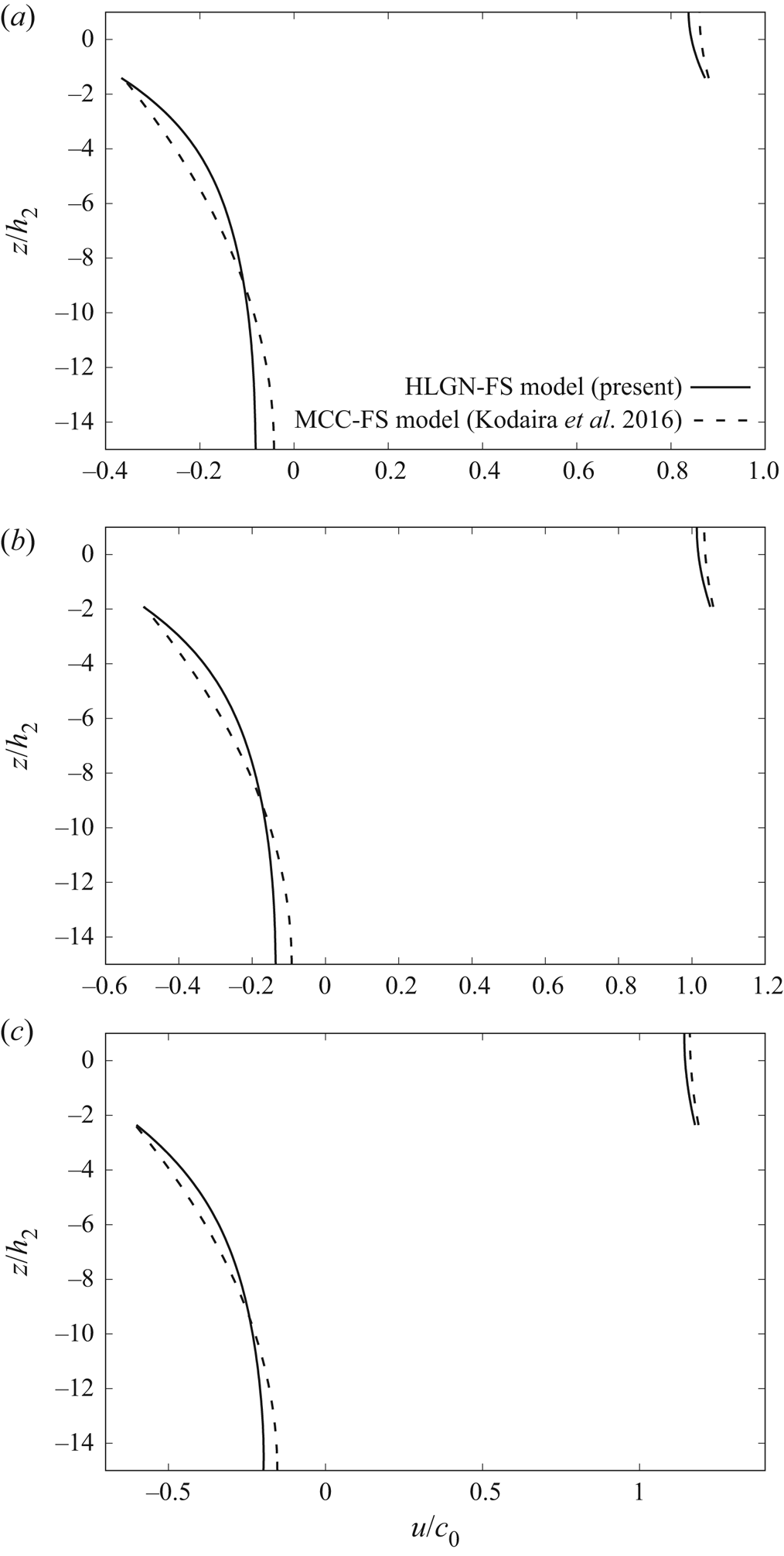
The horizontal velocity along the fluid column at the maximal displacement is presented in figure 21, where the MCC-FS results and the HLGN-FS results are included. Some differences appear between the MCC-FS results and the HLGN-FS results for this deep-configuration case. For the upper-layer horizontal velocity, the horizontal velocity predicted by the MCC-FS model is larger than that obtained by the HLGN-FS model. Meanwhile, for the lower-fluid layer near the maximal displacement, the horizontal velocity obtained by the MCC-FS model is larger than that obtained by the HLGN-FS model. Near the bottom, the MCC-FS model predicts smaller horizontal velocity than that of the HLGN-FS model.
Horizontal velocity along the fluid column at the maximal displacement,  $\rho _2/\rho _1=0.869$,
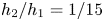 $h_2/h_1=1/15$ and (a)
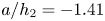 $a/h_2=-1.41$, (b)
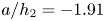 $a/h_2=-1.91$ and (c)
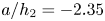 $a/h_2=-2.35$.

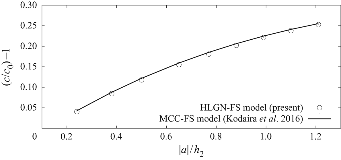
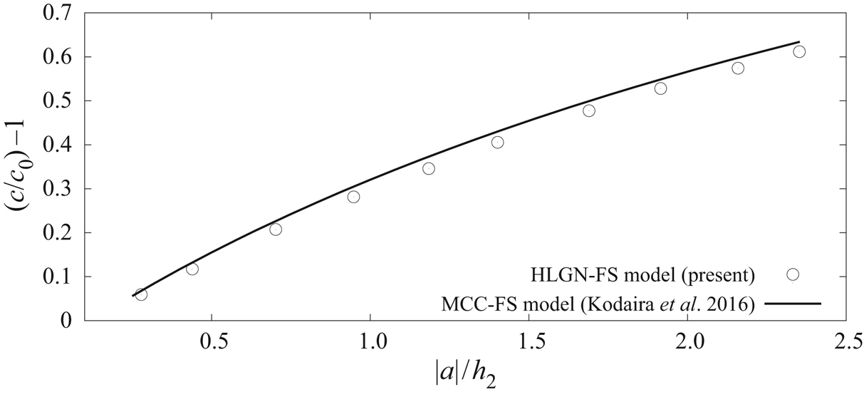
Variations of the excess wave speed with the wave amplitude obtained by the HLGN-FS model and the MCC-FS model are shown in figure 22. The wave speed predicted by the MCC-FS model is slightly larger than that obtained by the HLGN-FS model.
Excess propagation speed  $(c/c_0)-1$ versus amplitude,
 $\rho _2/\rho _1=0.869$ and
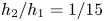 $h_2/h_1=1/15$.

For this case, we find that the MCC-FS results do not agree well with the present experimental data. Meanwhile, the HLGN-FS model is shown to be accurate to describe the internal solitary waves with a free surface in this case.
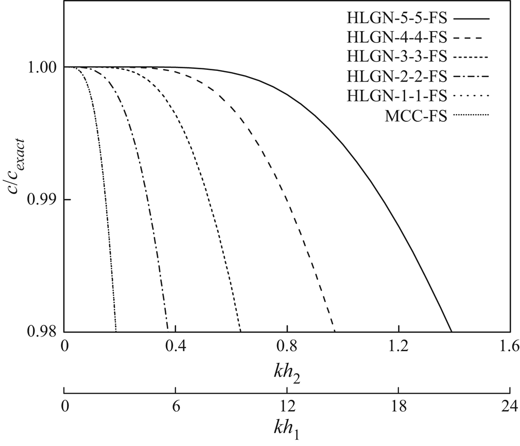
To further assess the differences between the HLGN-FS and the MCC-FS results, the linear dispersion relation of the HLGN-FS model with different levels is compared with the exact linear dispersion relation (Ten & Kashiwagi Reference Ten and Kashiwagi2004), given as
 \begin{equation} K {(}k\sinh kh - K\cosh kh {) }+ \varepsilon {(K^2 }- k {^2) \sinh kh_1 \sinh kh_2 }= 0, \end{equation}
where  $K=\omega ^2 /g$,
 $h=h_1+h_2$ and
 $\varepsilon =1-(\rho _2/\rho _1)$. The accuracy of the HLGN-FS model with different levels is shown in figure 23 for the case of
 $\rho _2/\rho _1=0.869$ and
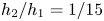 $h_2/h_1=1/15$.
Accuracy of the linear dispersion relations of the HLGN-FS model and the MCC-FS model, compared with the exact linear dispersion relation (Ten & Kashiwagi Reference Ten and Kashiwagi2004),  $\rho _2/\rho _1=0.869$ and
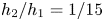 $h_2/h_1=1/15$. The MCC-FS and the HLGN-1-1-FS results are on top of each other.

Also shown in figure 23 is the accuracy of the linear dispersion relation of the MCC-FS model. The MCC-FS and the HLGN-1-1-FS results are on top of each other, and they predict the wave speed well for waves with  $kh_1<3$. It is observed that the higher level of the HLGN-FS model provides better agreement with the exact results for larger values of
 $kh_1$. The wave speed calculated by the HLGN-5-5-FS model is within
 $2\,\%$ error of the exact solution for waves with
 $kh_1<20$. Following the definition of the half-amplitude point
 $\lambda _{0.5}$ by Koop & Butler (Reference Koop and Butler1981), and based on the present experimental results, we estimate that, for the cases of
 $a/h_2=-1.41, -1.91$ and
 $-2.35$ in this subsection,
 $kh_1$ is approximately
 $17$,
 $14$ and
 $13$, respectively. Shown in figure 23, the MCC-FS model and the HLGN-1-1-FS model do not predict these internal solitary waves accurately for deep configurations. The high-level HLGN-FS models, for example the HLGN-5-5-FS model, predict the internal solitary waves accurately for both shallow and deep configurations.
6. Conclusions
In this study, large-amplitude internal solitary waves in a two-layer fluid system with a free surface are investigated by use of experimental and theoretical approaches. Laboratory experiments are conducted for some strongly nonlinear, deep-configuration, internal solitary-wave cases. Upon comparison of existing numerical solutions of the problem, including the MCC-FS model proposed by Kodaira et al. (Reference Kodaira, Waseda, Miyata and Choi2016), it was found that the existing numerical models do not provide accurate results under such conditions. This formed the motivation for developing a two-layer fluid model based on the high-level Green–Naghdi equations, which can also include the free-surface effects, namely the HLGN-FS model; a model that is applicable to both deep-water and shallow-water configurations. Comparisons of the results of the HLGN-FS model with the laboratory experiments show excellent agreement.
We apply the HLGN-FS model to study the internal solitary waves for three cases, and consider the wave profile, velocity field and wave speed. The conclusions are as follows:
When the density ratio between the two fluids with constant densities is close to  $1$ (e.g.
 $\rho _2/\rho _1=0.977$, case 1), the rigid-lid assumption is reasonable. For larger density differences (e.g.
 $\rho _2/\rho _1=0.859$, case 2; and
 $\rho _2/\rho _1=0.869$, case 3), the free-surface effects must be included.
For the strongly nonlinear, shallow-configuration case (e.g.  $\rho _2/\rho _1=0.859$ and
 $h_2/h_1=1/5$, case 2), the HLGN-FS model and the MCC-FS model both provide accurate solutions of the internal solitary waves with a free surface.
For the strongly nonlinear, deep-configuration case (e.g.  $\rho _2/\rho _1=0.869$ and
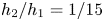 $h_2/h_1=1/15$, case 3), the HLGN-FS results match the experimental data much better than those provided by the MCC-FS model. Thus, the HLGN-FS model is shown to be accurate for describing the internal solitary waves for both shallow and deep configurations with a free surface.
Acknowledgments
The first and third authors’ (B.B.Z. and W.Y.D.) work is supported by the National Natural Science Foundation of China (Nos. 51490671, 11572093), the International Science and Technology Cooperation Project sponsored by the National Ministry of Science and Technology of China (No. 2012DFA70420) and the Special Fund for Basic Scientific Research of Central Colleges (Harbin Engineering University). The authors are grateful to the anonymous referees for their comments that improved our paper.
Declaration of interests
The authors report no conflict of interest.