1. Introduction
Microswimmers refer to microscopic entities capable of autonomous motion in fluids, including microorganisms (Durham & Stocker Reference Durham and Stocker2012) and synthetic self-propelled particles (Lauga Reference Lauga2020). In nature, many algae play an important ecological role as primary producers (Zeng et al. Reference Zeng, Zhang, Wu, Li and Wang2019; Muñoz & Guieysse Reference Muñoz and Guieysse2006). They are not only the main energy source in aquatic ecosystems (Richerson, Armstrong & Goldman Reference Richerson, Armstrong and Goldman1970; Round Reference Round1981) but can also be harnessed as bio-resources in general and biofuels in particular (Chisti Reference Chisti2007; Mata, Martins & Caetano Reference Mata, Martins and Caetano2010; Bees & Croze Reference Bees and Croze2014), offering significant economic value. However, excessive algal growth in water bodies can lead to aquatic disasters such as algal blooms and red tides (Durham, Kessler & Stocker Reference Durham, Kessler and Stocker2009; Steinbuck et al. Reference Steinbuck, Stacey, McManus, Cheriton and Ryan2009; Zeng, Jiang & Pedley Reference Zeng, Jiang and Pedley2022), posing threats to the environment and human health. Therefore, understanding the growth and dispersal mechanisms of algae is crucial for ecological management and environmental protection. On the other hand, synthetic active microswimmers, such as microrobots and nanoparticles for targeted drug delivery (Ghosh et al. Reference Ghosh, Misko, Marchesoni and Nori2013; Medina-Sánchez et al. Reference Medina-Sánchez, Magdanz, Guix, Fomin and Schmidt2018; Wu et al. Reference Wu, Chen, Mukasa, Pak and Gao2020; Michelin Reference Michelin2023), are gaining significant interest in scientific research. These microswimmers can precisely locate and release drugs within the body, enhancing therapeutic efficiency and efficacy. Additionally, microrobots have promising applications in environmental monitoring and pollution control (Urso & Pumera Reference Urso and Pumera2022; yi Hou et al. Reference yi Hou, tao Liu, ting Huang, biao Wu and lin Zhang2024). Investigating the movement mechanisms and control methods of these synthetic microswimmers helps to advance their application in medical and environmental sciences (Chen et al. Reference Chen, Jiang, Guo, Zeng and Guan2025). By studying both natural and synthetic active microswimmers in depth, we can better understand their behaviour and impacts in different environments, thereby developing more effective technologies and strategies to address associated ecological and health challenges.
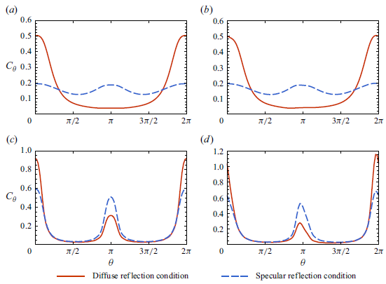
One of the research fields that has garnered increasing attention is the influence of different boundary conditions on the migration and distribution patterns of microswimmers (Berke et al. Reference Berke, Turner, Berg and Lauga2008; Li & Tang Reference Li and Tang2009; Sipos et al. Reference Sipos, Nagy, Di Leonardo and Galajda2015a ; Bianchi et al. Reference Bianchi, Saglimbeni, Frangipane, Dell’Arciprete and Leonardo2019; Buchner et al. Reference Buchner, Muller, Mehmood and Tam2021). Wall aggregation is a typical phenomenon common to many microbial suspensions. Rothschild (1963) first observed the wall-accumulation phenomenon in bull sperm swimming within a glass chamber. Berke et al. (Reference Berke, Turner, Berg and Lauga2008) similarly observed this phenomenon using bacterial suspensions. To characterise this phenomenon, researchers have proposed complex particle–wall interaction models (Spagnolie & Lauga Reference Spagnolie and Lauga2012; Sipos et al. Reference Sipos, Nagy, Di Leonardo and Galajda2015a ) as well as simpler non-interaction models, such as the Robin boundary condition (Enculescu & Stark Reference Enculescu and Stark2011; Elgeti & Gompper Reference Elgeti and Gompper2013; Ezhilan, Alonso-Matilla & Saintillan Reference Ezhilan, Alonso-Matilla and Saintillan2015; Jiang & Chen Reference Jiang and Chen2019; Peng & Brady Reference Peng and Brady2020) commonly used in numerical studies to describe the behaviour of particles sliding along the surface after colliding with the boundary. In recent years, some studies have also employed reflection boundary conditions (Bearon, Hazel & Thorn Reference Bearon, Hazel and Thorn2011; Volpe, Gigan & Volpe Reference Volpe, Gigan and Volpe2014; Ezhilan & Saintillan Reference Ezhilan and Saintillan2015; Jiang & Chen Reference Jiang and Chen2021; Wang, Jiang & Chen Reference Wang, Jiang and Chen2022; Guan et al. Reference Guan, Jiang, Wang, Zeng, Li and Chen2023) to characterise wall reflection behaviour. Buchner et al. (Reference Buchner, Muller, Mehmood and Tam2021) experimentally found that, in non-contact modes, the hydrodynamics dominated the interactions between Chlamydomonas reinhardtii and the walls, with the incident angle equalling the reflection angle. In addition to these phenomena, the experiment also observed that the swimming angles of microswimmers may exhibit scattering patterns (Drescher et al. Reference Drescher, Dunkel, Cisneros, Ganguly and Goldstein2011; Kantsler et al. Reference Kantsler, Dunkel, Polin and Goldstein2013), where the incident angle is independent of the reflection angle. Cisneros et al. (Reference Cisneros, Kessler, Ganguly and Goldstein2011) observed that, when bacteria collided with an inertial object, the flagellar bundles might spread apart and recombine, and then the bacteria would continue swimming at some arbitrary angle. Kantsler et al. (Reference Kantsler, Dunkel, Polin and Goldstein2013) showed that Chlamydomonas cells reflect off walls primarily through direct contact of their flagella, producing exit angles that vary arbitrarily. Contino et al. (Reference Contino, Lushi, Tuval, Kantsler and Polin2015) observed that random scattering interactions, long-lasting collisions of microalgae with boundaries, allow flagella to make multiple direct interactions with the surrounding surface, resulting in a uniform distribution of reflection angles across the available range of values, independent of the incidence angles. Jakuszeit & Croze (Reference Jakuszeit and Croze2024) demonstrated that Escherichia coli scattered off micropillars at angles that were broadly distributed and independent of the angle of incidence, significantly enhancing their effective diffusivity in confined environments. van Baalen et al. (Reference van Baalen, Uspal, Popescu and Isa2023) found that synthetic Janus particles exhibited a transition from orbiting behaviour to random scattering by tuning the chemical activity, further confirming that boundary interactions can yield near-uniform angular distributions of outgoing trajectories. Despite these complexities, most theoretical studies currently employ Robin or specular reflection boundary conditions, which cannot accurately capture these other types of boundary influences. Only a few studies have explored other boundary conditions, primarily employing Brownian dynamics simulation methods. Kumar et al. (Reference Kumar, Thomson, Powers and Harris2021) used random reflection collision conditions for rod-shaped particles in Brownian dynamics simulations, assuming that the angle distribution of particles after they collide with the wall is randomly distributed. Maretvadakethope et al. (Reference Maretvadakethope, Hazel, Vasiev and Bearon2023) were the first to employ Dirichlet boundary conditions in a continuum model to describe random reflection of active particles at boundaries, setting the value of the probability density function at the boundary to be the same constant and without explicitly imposing a zero-flux condition. Using a Galerkin finite element method and validating against individual-based model simulations, they focused on the concentration distribution in the regime where the microswimmer swimming speed is much smaller than the flow velocity, while considering only steady-state results and neglecting streamwise migration.
In describing the transport processes of microswimmers, both individual-based and continuum models are commonly employed. Individual-based models, which incorporate the Jeffery equation (Jeffery & Filon Reference Jeffery and Filon1922) and rely on Brownian dynamics simulations of numerous particle trajectories, play a crucial role in elucidating the mechanisms of microbial aggregation and migration under complex flow conditions. Classic continuum models include the Pedley–Kessler (PK) model (Pedley & Kessler Reference Pedley and Kessler1990) and the generalized Taylor dispersion (GTD) model (Frankel & Brenner Reference Frankel and Brenner1989). All the models assume that particles reach a quasi-steady state in the rotational space, from which the probability density function of their swimming directions is obtained. By averaging over this directional distribution, one can determine the local drift velocity. The GTD model employs generalised Taylor dispersion theory to calculate the effective swimming diffusion tensor, making it more accurate in conditions of strong shear (Bearon, Bees & Croze Reference Bearon, Bees and Croze2012; Croze, Bearon & Bees Reference Croze, Bearon and Bees2017; Fung, Bearon & Hwang Reference Fung, Bearon and Hwang2020). These two types of models have wide applications (Manela & Frankel Reference Manela and Frankel2003; Bearon et al. Reference Bearon, Bees and Croze2012; Hwang & Pedley Reference Hwang and Pedley2014; Zeng & Pedley Reference Zeng and Pedley2018; Fung et al. Reference Fung, Bearon and Hwang2020), but may fail when the swimming scale is relatively large compared with the confined environment or when boundary effects are significant (Jiang & Chen Reference Jiang and Chen2020; Fung, Bearon & Hwang Reference Fung, Bearon and Hwang2022; Wang, Jiang & Chen Reference Wang, Jiang and Chen2023).
The general continuum model is based on the Smoluchowski equation (Doi & Edwards Reference Doi and Edwards1988), which describes the evolution of particle number density in a high-dimensional phase space that encompasses both rotational and positional coordinates. Unlike the PK and GTD models, the Smoluchowski equation assigns equal importance to both translational and rotational processes. However, its high dimensionality makes direct solutions challenging (Saintillan & Shelley Reference Saintillan and Shelley2008). To address this issue, some researchers have employed multiple time-scale methods (Mei, Auriault & Ng Reference Mei, Auriault and Ng1996; Latini & Bernoff Reference Latini and Bernoff2001; Wu & Chen Reference Wu and Chen2014; Guan & Chen Reference Guan and Chen2024). Bearon & Hazel (Reference Bearon and Hazel2015) employed a multiple time-scale analysis to derive an effective drift velocity, thereby providing an explanation for high-shear-trapping phenomena. Vennamneni, Nambiar & Subramanian (Reference Vennamneni, Nambiar and Subramanian2020) extended the multi-time-scale model towards a drift-diffusion framework that enabled a deeper investigation of both high-shear and low-shear-trapping phenomena. Others have combined the Smoluchowski equation with the concentration moment method (Aris Reference Aris1956; Chatwin Reference Chatwin1970; Barton Reference Barton1983). The moment method is used to transform the dynamical description of a distribution function or complex system into a set of simple moment equations, as most frequently employed in solving dispersion problems (Yasuda Reference Yasuda1984; Bello, Rezzonico & Righetti Reference Bello, Rezzonico and Righetti1994; Bees & Croze Reference Bees and Croze2010; Bearon et al. Reference Bearon, Bees and Croze2012; Croze et al. Reference Croze, Sardina, Ahmed, Bees and Brandt2013). Based on the moment method as supported by the generalised Taylor dispersion theory, Jiang & Chen (Reference Jiang and Chen2019) presented direct solutions for the asymptotic dispersion problem of active particles in some typical confined shear flows. Consequently Jiang & Chen (Reference Jiang and Chen2021) further used the biorthogonal expansion method to solve the transient probability density moment equations of various orders.
Regarding the phenomenon of particles exhibiting randomly reflection upon contacting surfaces, this work seeks to explore the effect of a diffuse reflection boundary condition in characterising the dispersion process of microswimmers by the general continuum model. Based on the Smoluchowski equation and the moment method, this paper solves the long-term asymptotic solution and the transient solution, respectively. Comparisons are made with numerical simulations to explore specific phenomena under different parameter conditions, including low-shear trapping, downstream migration and centreline aggregation.
Our work is illustrated primarily for microswimmers with elongated shapes. Compared with spherical particles, ellipsoidal active particles typically exhibit more heterogeneous distributions in shear flows (Wang et al. Reference Wang, Jiang, Zeng and Chen2025). This is primarily due to shape-induced variations in angular velocity (Jeffery & Filon Reference Jeffery and Filon1922; Brenner Reference Brenner1967), causing ellipsoidal particles to adjust their swimming directions more slowly near regions of principal strain, thereby concentrating their orientation distributions. In Poiseuille flow, ellipsoidal particles display a range of intriguing phenomena. Their cross-sectional concentration distributions may, for example, appear as a high-shear-trapping state (Rusconi, Guasto & Stocker Reference Rusconi, Guasto and Stocker2014; Bearon & Hazel Reference Bearon and Hazel2015; Ezhilan & Saintillan Reference Ezhilan and Saintillan2015; Vennamneni et al. Reference Vennamneni, Nambiar and Subramanian2020) or transition into various low-shear-trapping states, including centreline depletion (Rusconi et al. Reference Rusconi, Guasto and Stocker2014; Bearon & Hazel Reference Bearon and Hazel2015; Ezhilan et al. Reference Ezhilan, Alonso-Matilla and Saintillan2015) and centreline accumulation (Barry et al. Reference Barry, Rusconi, Guasto and Stocker2015; Guan et al. Reference Guan, Jiang, Tao, Chen and Lee2024). Another classic behaviour is their rheotaxis (Miki & Clapham Reference Miki and Clapham2013), encompassing both downstream (Dehkharghani et al. Reference Dehkharghani, Waisbord, Dunkel and Guasto2019) and upstream migration (Hill et al. Reference Hill, Kalkanci, McMurry and Koser2007; Mathijssen et al. Reference Mathijssen, Shendruk, Yeomans and Doostmohammadi2016; Figueroa-Morales et al. Reference Figueroa-Morales, Rivera, Soto, Lindner, Altshuler and Clément2020; Omori et al. Reference Omori, Kikuchi, Schmitz, Pavlovic, Chuang and Ishikawa2022).
The structure of this paper is as follows. Section 2 introduces the transport problem of microswimmers under diffuse reflection boundary conditions. Section 3 presents the asymptotic and transient solutions of the transport problem. Section 4 considers the influence of factors such as flow velocity, swimming velocity, shape factor and gravity-induced torque strength on the asymptotic concentration and orientation distributions. Section 5 examines the transient concentration distribution, drift velocity and dispersivity under different initial release conditions. Finally, § 6 provides conclusions and outlook. Numerical validation using the random walk method is presented in Appendix A, comparisons with results under other boundary conditions are provided in Appendix B and details of the biorthogonal expansion method are presented in Appendix C.
2. Formulation
2.1. Governing equations
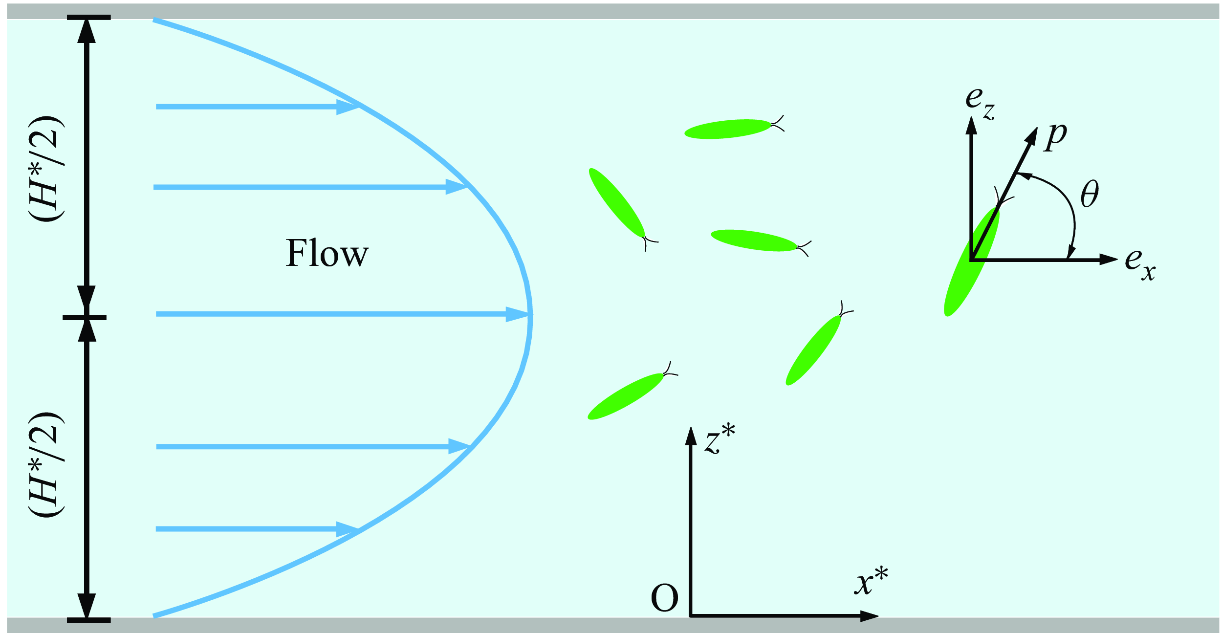
Sketch of a dilute suspension of ellipsoidal microswimmers in a plane Poiseuille flow.

As shown in figure 1, we consider a two-dimensional laminar flow in a channel of depth
 $H^{\ast }$
, with position coordinates
 $(x^{\ast }, z^{\ast })$
and corresponding base vectors
 $(\boldsymbol{e}_x, \boldsymbol{e}_z)$
, along with an orientation coordinate
 $\theta$
. We assume that the suspension of microswimmers is dilute enough to justify neglecting their mutual interactions as well as their impact on the background flow (Bees Reference Bees2020). Under these conditions, the evolution of the probability density function for the population can be described by the Smoluchowski equation (Doi & Edwards Reference Doi and Edwards1988)
 \begin{equation} \begin{aligned} \frac {\partial P}{\partial t^{\ast }} + \boldsymbol{\nabla }_R^{\ast } \boldsymbol{\cdot } \left [\left (u^{\ast } (z^{\ast })\boldsymbol{e}_x + V_s^{\ast } \boldsymbol{p} \right )P - D_t^{\ast } \boldsymbol{\nabla }_R^{\ast }P\right ] + \boldsymbol{\nabla }_p \boldsymbol{\cdot } (\boldsymbol{\dot {p}}^{\ast } P - D_r^{\ast } \boldsymbol{\nabla }_p P) = 0, \end{aligned} \end{equation}
where
 $P$
is the probability of finding a microswimmer at the position-and-orientation point
 $(x^{\ast },z^{\ast },\theta )$
at time
 $t^{\ast }$
;
 $\boldsymbol{\nabla }_R^{\ast }$
and
 $\boldsymbol{\nabla }_p$
are defined as the gradient operator
 $({\partial }/{\partial x^{\ast }}) \boldsymbol{e}_x + ({\partial }/{\partial z^{\ast }}) \boldsymbol{e}_z$
and
 $({\partial }/{\partial \theta }) \boldsymbol{e}_{\theta }$
in the position and orientation space;
 $u^{\ast }(z^{\ast })$
is the velocity of the unidirectional shear flow;
 $V_s^{\ast }$
is the constant swimming speed of the microswimmers;
 $\boldsymbol{p}$
is the swimming direction unit vector of the microswimmers consistent with the major axis direction;
 $D_t^{\ast }$
and
 $D_r^{\ast }$
represent the randomness in microswimmers’ position and orientation resulting from biological variation in their motility, including both thermal and athermal sources; ignoring inertial motion and considering gyrotaxis,
 $\dot {\boldsymbol{p}^{\ast }}$
is the rate of change of swimming direction governed by the Jeffery equation (Jeffery & Filon Reference Jeffery and Filon1922; Hinch & Leal Reference Hinch and Leal1972)
 \begin{equation} \dot {\boldsymbol{p}^{\ast }}=\frac {\textrm{d} \boldsymbol{p}^{\ast }}{\textrm{d} t^{\ast }}= \boldsymbol{\varOmega }_m^{\ast } \times \boldsymbol{p} =\left \{ \frac {1}{2B^{\ast }} \boldsymbol{p} \times \boldsymbol{k} + \frac {1}{2} \boldsymbol{\omega }^{\ast } +\alpha _0 [\boldsymbol{p} \times (\boldsymbol{E}^{\ast }\boldsymbol{\cdot } \boldsymbol{p})]\right \} \times \boldsymbol{p}, \end{equation}
where
 \begin{align} \boldsymbol{\omega }^{\ast } = \boldsymbol{\nabla }_R^{\ast } \times \boldsymbol{u}^{\ast } ,\end{align}
and
 \begin{align} \boldsymbol{E}^{\ast } = \tfrac{1}{2} \left [\boldsymbol{\nabla }_R^{\ast } \boldsymbol{u}^{\ast } +(\boldsymbol{\nabla }_R^{\ast } \boldsymbol{u}^{\ast } )^{\textrm{T}}\right ] ,\end{align}
are the vorticity and rate-of-strain tensor of the flow, respectively,
 $\boldsymbol{\varOmega }_m^{\ast }$
is the total angular velocity of the microswimmers,
 $B^{\ast }$
is the gravitactic reorientation time and
 $\alpha _0$
is the shape factor of the microswimmers ranging from
 $0$
(spherical) to
 $1$
(rod-like). We define the following dimensionless variables:
 \begin{equation} \left . \begin{aligned} t &= t^{\ast } D^{\ast }_r, & \mathit{Pe}_s &= \frac {V_s^{\ast }}{D^{\ast }_r H^{\ast }}, & \mathit{Pe}_f &= \frac {u^{\ast }_m}{D^{\ast }_r H^{\ast }}, & u &= \frac {u^{\ast }}{u^{\ast }_m} -1 ,& \\ x &= \frac {x^{\ast }-u^{\ast }_m t^{\ast }}{H^{\ast }}, & z &= \frac {z^{\ast }}{H^{\ast }}, & \lambda &= \frac {1}{2B^{\ast } D_r^{\ast }},& D_t &= \frac {D_t^{\ast }}{D_r^{\ast }{H^{\ast }}^2},& \end{aligned} \!\!\!\right \} \end{equation}
where
 $\textit{Pe}_{s}$
is the swimming Péclet number comparing the swimming ability of the microswimmers, or equivalently the strength of confinement;
 $\textit{Pe}_{\!f}$
is the flow Péclet number representing the flow rate;
 $\lambda$
is the dimensionless inverse of the gravitactic times scale
 $B^{\ast }$
;
 $D_t$
is the ratio of translational diffusion decorrelation time scale to rotational diffusion reorientation time scale;
 $u_m^{\ast }$
is the average flow velocity given as
 \begin{equation} u_m^{\ast } \triangleq \frac {1}{H^{\ast }} \int _0^{H^{\ast }} u^{\ast }(z^{\ast }) \, \textrm{d} z^{\ast }. \end{equation}
The dimensionless form of the probability conservation equation (2.1) becomes
 \begin{equation} \frac {\partial P}{\partial t} + [\textit{Pe}_{\!f} u(z)+\textit{Pe}_{s}\cos \theta ] \frac {\partial P}{\partial x} -D_t\frac {\partial ^2 P}{\partial x^2} = \mathcal{L}P, \end{equation}
where
 $\mathcal{L}P$
is the flux in space
 $\{z,\theta \}$
 \begin{equation} \mathcal{L}(\boldsymbol{\cdot }) \, \triangleq \, D_t\frac {\partial ^2 (\boldsymbol{\cdot })}{\partial z^2} - \textit{Pe}_{s} \sin \theta \frac {\partial (\boldsymbol{\cdot })}{\partial z} - \frac {\partial (\dot {\theta }(\boldsymbol{\cdot }))}{\partial \theta } + \frac {\partial ^2 (\boldsymbol{\cdot })}{\partial \theta ^2}. \end{equation}
The angular velocity is governed by the Jeffery equation, and the dimensionless rate of change of swimming direction
 $\theta$
is
 \begin{equation} \dot {\theta }=\frac {1}{2}\textit{Pe}_{\!f} \frac {\textrm{d} u}{\textrm{d} z}(-1+ \alpha _0 \cos 2 \theta ) + \lambda \cos \theta . \end{equation}
This paper considers Poiseuille flow, the dimensionless flow velocity is given in the coordinate system moving at the mean flow velocity as
 \begin{equation} u(z)=-6z^2+6z-1. \end{equation}
2.2. Boundary condition
In the study of microswimmer dynamics, appropriate boundary conditions are essential for accurately capturing particle–wall interactions and developing reliable theoretical models. These boundary conditions not only affect the mathematical well posedness of the problem but also have significant physical implications on phenomena such as accumulation, orientation distribution and overall transport properties of the microswimmers.
In the absence of microswimmer loss or generation at the boundaries, a zero-flux condition should be imposed to ensure the conservation of microswimmers (Ezhilan, Pahlavan & Saintillan Reference Ezhilan, Pahlavan and Saintillan2012; Bearon & Hazel Reference Bearon and Hazel2015)
 \begin{equation} \int _0^{2\pi } \left (\textit{Pe}_{s} \sin \theta P - D_t \frac {\partial P}{\partial z}\right ) \textrm{d} \theta = 0, \quad \textrm{at} \; z=0,1 . \end{equation}
Specifically, it means that the total probability flux of the microswimmers at the boundary is zero, which includes the probability flux due to swimming and the probability flux due to translational diffusion. The zero-flux condition is given in an integral form and inherently lacks the detailed local information necessary to fully specify a unique solution to the Smoluchowski equation (Bearon & Hazel Reference Bearon and Hazel2015; Ezhilan & Saintillan Reference Ezhilan and Saintillan2015). Specifically, integral boundary conditions define only the global relationship of fluxes or particle distributions at boundaries but do not specify explicitly how particles interact locally with the boundary. Multiple local boundary conditions, such as the Robin condition (Wang et al. Reference Wang, Jiang, Chen, Tao and Li2021), specular reflection condition (Jiang & Chen Reference Jiang and Chen2019) or diffuse reflection conditions, could fulfil the same integral boundary requirement. So the zero-flux condition is not sufficient to ensure the uniqueness of the solution to the partial differential equation; therefore, stronger conditions are required to enforce this.
In current theoretical analyses, two classic types of boundary conditions are primarily considered: the Robin condition and the specular reflection condition, both of which provide different frameworks for modelling particle–wall interactions. The Robin condition is a boundary condition used to describe the accumulation of particles on the wall surface, representing the balance between the probability flux due to particle swimming and the probability flux due to translational diffusion; this condition effectively captures the tendency of active particles to gather near surfaces due to their self-propelled motion and diffusive behaviour. Conversely, the specular reflection condition is a boundary condition used to describe particles bouncing off the wall, indicating that the reflection angle of the particle after hitting the wall is equal to the angle of incidence, similar to how a billiard ball reflects off the edge of a pool table.
However, the swimming behaviour of microswimmers near boundaries can be highly complex (Cisneros et al. Reference Cisneros, Dombrowski, Goldstein and Kessler2006; Sipos et al. Reference Sipos, Nagy, Di Leonardo and Galajda2015b ; Bianchi, Saglimbeni & Di Leonardo Reference Bianchi, Saglimbeni and Di Leonardo2017; Lushi, Kantsler & Goldstein Reference Lushi, Kantsler and Goldstein2017), especially after collisions. In addition to the phenomena of aggregation and specular reflection at walls, some experiments have observed that microswimmers, upon colliding with a surface, swim off at arbitrary angles, with the exit angle randomly distributed and independent of the incident angle (Kantsler et al. Reference Kantsler, Dunkel, Polin and Goldstein2013; Contino et al. Reference Contino, Lushi, Tuval, Kantsler and Polin2015; van Baalen et al. Reference van Baalen, Uspal, Popescu and Isa2023; Jakuszeit & Croze Reference Jakuszeit and Croze2024). Traditional approaches, such as using Robin or specular reflection boundary conditions in continuum models, are unable to accurately capture this physical phenomenon. Currently, theoretical studies exploring such boundary conditions remain limited (Kumar et al. Reference Kumar, Thomson, Powers and Harris2021; Maretvadakethope et al. Reference Maretvadakethope, Hazel, Vasiev and Bearon2023), indicating that the impact of boundary behaviour on microswimmer transport is still not fully understood.
To address this, our paper employs a continuum model with diffuse reflection boundary conditions to describe the specific interactions of microswimmers when they encounter a wall and reflect at arbitrary angles (similar to the diffuse reflection phenomenon of light). Ignoring hydrodynamic interactions with boundary, we assume that microswimmers reflect randomly (i.e. the reflection angles are uniformly distributed) upon reaching the boundary, and that the reflection after hitting the boundary is instantaneous (i.e. the residence time at the boundary is not considered). In the theoretical model, we further assume at the boundary in position space that the probability density is independent of angle, meaning the angular distribution is uniform
 \begin{equation} \frac {\partial P}{\partial \theta }(x,z,\theta ,t) = 0 \quad \textrm{at} \; z = 0, 1. \end{equation}
Additionally, to satisfy the zero-flux condition, we need to employ an integral condition, which indicates that the total flux caused by translational diffusion at the boundary is zero
 \begin{equation} \int _0^{2\pi } \frac {\partial P}{\partial z}(x,z,\theta ,t) \; \textrm{d} \theta = 0, \quad \textrm{at} \; z=0,1. \end{equation}
From a mathematical point of view, we decompose the zero-flux condition (2.11) into two parts: the probability flux due to particle swimming at the boundary and the probability flux due to translational diffusion, both of which are set to zero. We then strengthen the former condition, requiring that the probability at the boundary is uniformly distributed in the orientation space.
In the orientation space,
 $\theta$
refers to the angle between the microswimmer’s swimming direction and the
 $x$
-axis, which is a periodic variable. The natural periodic boundary conditions of
 $P$
are imposed as
 \begin{equation} \left .\begin{aligned} P(x,z,\theta ,t) &= P(x,z,\theta +2\pi ,t), \\ \frac {\partial P}{\partial \theta }(x,z,\theta ,t) &= \frac {\partial P}{\partial \theta }(x,z,\theta +2\pi ,t), \end{aligned} \right \} \end{equation}
valid for
 $0\leqslant z \leqslant 1$
and
 $0\leqslant \theta \lt 2\pi$
.
3. Solution
3.1. Moment equation
The Smoluchowski equation is high-dimensional (Saintillan & Shelley Reference Saintillan and Shelley2008), making direct solutions very challenging. By transforming the Smoluchowski equation into the corresponding moment equations, it is possible to reduce the dimensionality of the equations while still retaining the statistical information about the local distribution of particles. The core idea of the moment method is to calculate the moments of a distribution function (such as a probability density function) with respect to certain variables, and use these moments to describe the macroscopic properties of the system.
The local moments and total moments are defined as follows (Aris Reference Aris1956; Smith Reference Smith1985; Bees & Croze Reference Bees and Croze2010):
 \begin{align} P_n(z,\theta ,t) &\, \triangleq \, \int _{-\infty }^{\infty } x^n P \; \textrm{d} x,\quad n=0,1,\ldots,\\[-12pt]\nonumber\end{align}
 \begin{align} M_n(t) &\, \triangleq \, \int _0^1 \int _0^{2\pi } P_n(z,\theta ,t) \; \textrm{d} \theta \textrm{d}z \quad n=0,1,\ldots . \end{align}
With the classical finite release condition (Aris Reference Aris1956; Chatwin Reference Chatwin1970)
 \begin{equation} \begin{aligned} P \to 0 \quad \& \quad \frac {\partial ^n P}{\partial x^n} \to 0, \quad \mbox{as}\ |x| \to \infty ,\; n=1,2,\ldots , \end{aligned} \end{equation}
multiplying the governing equation (2.7) by
 $x^n$
and integrating over
 $x \in (-\infty ,\infty )$
, we get the following governing equations for
 $n$
th-order local moments
 $P_n$
:
 \begin{equation} \begin{aligned} \frac {\partial P_n}{\partial t} = n(n-1) D_t P_{n-2} + n (\textit{Pe}_{\!f} u + \textit{Pe}_{s} \cos \theta ) P_{n-1} + \mathcal{L} P_n, \quad n=0,1,\ldots . \end{aligned} \end{equation}
Here,
 $P_{-1}=P_{-2}=0$
is introduced so that all moment equations have the unified form.
3.2. Asymptotic solution
For the asymptotically steady state, this paper primarily focuses on the issue of clustering phenomena in the local space, where an exact solution can be obtained by solving the zeroth-order local space moment equation. The long-time asymptotic state of the zeroth-order longitudinal moment of
 $P$
is
 \begin{equation} P^{\infty }_0(z,\theta )=\lim _{t \to \infty } P_0(z,\theta ,t), \end{equation}
which represents the asymptotic local distribution. According to the GTD theory,
 $P^{\infty }_0$
satisfies
 \begin{equation} \mathcal{L}P^{\infty }_0(z,\theta )=0. \end{equation}
The boundary conditions of
 $P^{\infty }_0$
are the same as those of
 $P$
 \begin{equation} \left . \begin{aligned} \frac {\partial P^{\infty }_0}{\partial \theta } = 0, \quad \textrm{at} \; z = 0, 1,\\ \int _0^{2\pi } \frac {\partial P^{\infty }_0}{\partial z} \; \textrm{d} \theta = 0, \quad \textrm{at} \; z=0,1,\\ P^{\infty }_0(z,0) = P^{\infty }_0(z,2\pi ), \\ \frac {\partial P^{\infty }_0}{\partial \theta }(z,0) = \frac {\partial P^{\infty }_0}{\partial \theta }(z,2\pi ) . \end{aligned} \right \} \end{equation}
The normalisation condition is
 \begin{equation} \int _0^{1} \int _0^{2\pi } P^{\infty }_0(z,\theta ) \; \textrm{d} \theta \; \textrm{d} z =1. \end{equation}
The active propulsion of the microswimmers causes the operator
 $\mathcal{L}$
to be non-self-adjoint. This non-self-adjoint nature complicates the solution process, as it prevents the use of classical methods such as separation of variables and the method of characteristics. To overcome this challenge, we employ the Galerkin method (Doi & Edwards Reference Doi and Edwards1978; Hill & Bees Reference Hill and Bees2002; Manela & Frankel Reference Manela and Frankel2003) to obtain an approximate solution to the eigenvalue problem. The Galerkin method involves selecting a suitable set of basis functions and projecting the original problem onto a finite-dimensional subspace spanned by these basis functions. By doing so, the infinite-dimensional eigenvalue problem is transformed into a solvable system of algebraic equations. The complete function basis under the diffuse reflection condition (3.7) is constructed using the eigenfunctions of the Laplace operator
 $L = ({\partial ^2}/{\partial z^2}) + ({\partial ^2}/{\partial \theta ^2})$
, as detailed in § 3.4. Then we express the solution
 $P^{\infty }_0(z,\theta )$
as a linear combination of basis functions and formulate the equation in its weak form using inner products. The inner product of any two basis functions
 $f$
and
 $g$
is in the
 $L^2$
inner product form
 \begin{equation} \langle f, g \rangle \triangleq \int _0^1 \int _{0}^{2\pi } f(z, \theta ) g(z, \theta ) \, \textrm{d}\theta \, \textrm{d}z. \end{equation}
Under the premise of reasonable computational cost and ensuring convergence, we cut
 $n=80$
in the z direction and
 $m=20$
in the
 $\theta$
direction. The total number of basis functions (3.56) is 3281.
We define the asymptotically steady vertical distribution of longitudinally and orientationally accumulated concentration (hereafter abbreviated as vertical concentration distribution or simply vertical distribution) and steady orientation distribution of longitudinally and vertically accumulated concentration (hereafter abbreviated as orientation concentration distribution or simply orientation distribution) as follows:
 \begin{align} C_v(z) &\, \triangleq \, \int _0^{2\pi } P^{\infty }_0(z,\theta ) \; \textrm{d} \theta , \end{align}
 \begin{align} C_\theta (\theta ) &\, \triangleq \, \int _0^{1} P^{\infty }_0(z,\theta ) \; \textrm{d} z. \end{align}
By integrating the (3.6) over
 $\theta \in [0,2\pi ]$
, and applying the periodic boundary conditions in the orientation space, we obtain
 \begin{equation} \int _{0}^{2\pi } \left ( D_t \frac {\partial ^2 P^{\infty }_0}{\partial z^2} - \textit{Pe}_{s} \sin \theta \frac {\partial P^{\infty }_0}{\partial z} \right ) \textrm{d} \theta = 0. \end{equation}
Exchanging the order of differentiation and integration
 \begin{equation} \frac {\textrm{d} }{\textrm{d} z} \int _{0}^{2\pi } \left ( D_t \frac {\partial P^{\infty }_0}{\partial z} - \textit{Pe}_{s} \sin \theta P^{\infty }_0 \right ) \textrm{d} \theta = 0. \end{equation}
Then
 \begin{equation} \begin{aligned} \int _{0}^{2\pi } \left ( D_t \frac {\partial P^{\infty }_0}{\partial z} - \textit{Pe}_{s} \sin \theta P^{\infty }_0 \right ) \textrm{d}\theta \equiv C, \quad \forall 0 \lt z \lt 1, \end{aligned} \end{equation}
where
 $C$
represents a constant. The continuity of the solution requires that the vertical total flux at the boundary be equal
 \begin{equation} \begin{aligned} \int _{0}^{2\pi } \left ( D_t \frac {\partial P^{\infty }_0(0,\theta )}{\partial z} - \textit{Pe}_{s} \sin \theta P^{\infty }_0(0,\theta ) \right ) \textrm{d} \theta \\ =\int _{0}^{2\pi } \left ( D_t \frac {\partial P^{\infty }_0(1,\theta )}{\partial z} - \textit{Pe}_{s} \sin \theta P^{\infty }_0(1,\theta ) \right ) \textrm{d} \theta . \end{aligned} \end{equation}
Then
 \begin{equation} \int _{0}^{2\pi } \left ( D_t \frac {\partial P^{\infty }_0}{\partial z} - \textit{Pe}_{s} \sin \theta P^{\infty }_0 \right ) \textrm{d}\theta \equiv C, \quad \forall \, 0 \leqslant z \leqslant 1, \end{equation}
which indicates that the vertical total flux is constant across any region in the position space. At liquid–gas or liquid–solid interfaces, it is typically assumed that the vertical flux of particles is zero, then we have
 \begin{equation} \int _{0}^{2\pi } \left ( D_t \frac {\partial P^{\infty }_0}{\partial z} - \textit{Pe}_{s} \sin \theta P^{\infty }_0 \right ) \textrm{d}\theta \equiv 0, \quad \forall \, 0 \leqslant z \leqslant 1. \end{equation}
Thus, at the asymptotic steady state, the vertical flux is zero across any region in the position space. Using the above equation, we can also obtain
 \begin{equation} D_t \frac {\textrm{d}C_v}{\textrm{d}z} =\int _{0}^{2\pi } D_t \frac {\partial P^{\infty }_0}{\partial z}\; \textrm{d}\theta =\int _0^{2\pi } \textit{Pe}_{s} \sin \theta P^{\infty }_0(z,\theta ) \; \textrm{d} \theta = J_z. \end{equation}
That is, the up-swimming flux
 $J_z$
is proportional to gradient of the vertical concentration distribution, with the ratio being the translational diffusion coefficient. So we can determine the up-swimming flux at a certain point from the slope of the vertical concentration distribution curve.
3.3. Transient solution
In this paper, due to the computational load and the requirements for relevant statistics, we only solve up to the second moment. According to the moment equation (3.3), the governing equations for
 $P_0$
,
 $P_1$
and
 $P_2$
are, respectively
 \begin{align} \frac {\partial P_0}{\partial t} &= \mathcal{L} P_0,\\[-12pt]\nonumber\end{align}
 \begin{align} \frac {\partial P_1}{\partial t} &= \left (\textit{Pe}_{\!f} u + \textit{Pe}_{s} \cos \theta \right ) P_0 + \mathcal{L} P_1,\\[-12pt]\nonumber\end{align}
 \begin{align} \frac {\partial P_2}{\partial t} &= 2D_t P_0 + 2\left (\textit{Pe}_{\!f} u + \textit{Pe}_{s} \cos \theta \right ) P_1 + \mathcal{L} P_2. \\[9pt] \nonumber \end{align}
The boundary conditions of
 $P_n(n=0,1,2)$
are the same as those of
 $P$
 \begin{equation} \left . \begin{aligned} \frac {\partial P_n}{\partial \theta } = 0, \quad \textrm{at} \; z = 0, 1,\\ \int _0^{2\pi } \frac {\partial P_n}{\partial z} \; \textrm{d} \theta = 0, \quad \textrm{at} \; z=0,1,\\ P_n(z,0,t) = P_n(z,2\pi ,t), \\ \frac {\partial P_n}{\partial \theta }(z,0,t) = \frac {\partial P_n}{\partial \theta }(z,2\pi ,t) . \end{aligned} \right \} \end{equation}
The normalisation condition is
 \begin{equation} \int _0^{1} \int _0^{2\pi } P_n(z,\theta ) \; \textrm{d} \theta \; \textrm{d} z =1. \end{equation}
In the typical case of dispersion due to an instantaneous release at
 $x=0$
, the initial condition is taken as
 \begin{equation} \begin{aligned} P(x,z,\theta ,0) = \frac {1}{2\pi } \delta (x) P_{ic}(z), \end{aligned} \end{equation}
where
 $\delta$
is the Dirac delta function. Then the initial release conditions of
 $P_n(n=0,1,2)$
are
 \begin{equation} \begin{aligned} P_0(z,\theta ,0) = P_{ic}(z), \\ P_n(z,\theta ,0) = 0,\; n=1,2. \end{aligned} \end{equation}
We consider that the microswimmers are uniformly distributed in the swimming direction space at the initial moment. For the point source release condition, where microswimmers are released at a specific vertical position
 $z=z_0$
, we take
 $P_{ic}(z)=\delta (z-z_0)$
. For the line-source release condition, which corresponds to a uniform distribution in the vertical direction, we take
 $P_{ic}(z)=1$
. Note that the initial conditions all satisfy the boundary conditions. In the paper, we primarily consider the line-source release condition.
We first use the Galerkin method to approximately solve the eigenvalue problem of the operator
 $\mathcal{L}$
. Then, the local moment
 $P_n$
is expanded in terms of the eigenfunctions of
 $\mathcal{L}$
. To determine the expansion coefficients related to the initial conditions, we introduce the left eigenfunctions and the biorthogonality relation. For further details, refer to Appendix C.
The zeroth-order local moment defines the transient vertical distribution and transient orientation distribution
 \begin{align} C_t(z,t) &\, \triangleq \, \int _0^{2\pi } P_0(z,\theta ,t) \; \textrm{d} \theta , \end{align}
 \begin{align} C_{\varTheta }(\theta ,t) &\, \triangleq \, \int _0^1 P_0(z,\theta ,t) \; \textrm{d} z. \end{align}
Integrating the first and second local moments yields the first and second total moments, which define the transient drift velocity and dispersivity in the locally averaged sense
 \begin{align} U_d(t) &\, \triangleq \, \frac {\textrm{d} M_1}{\textrm{d} t}, \end{align}
 \begin{align} D_T(t) &\, \triangleq \, \frac {1}{2}\frac {\textrm{d} \left(M_2 - M_1^2\right)}{\textrm{d} t}. \\[9pt] \nonumber \end{align}
According to the boundary conditions (3.22), we can get
 \begin{equation} \int _0^{1} \int _0^{2\pi } \mathcal{L} P_n(z,\theta ,t) \; \textrm{d} \theta \; \textrm{d} z =0. \end{equation}
Using the condition (3.30) and integrating the (3.19), we can obtain the governing equation for the global moment
 \begin{align} \frac {\textrm{d} M_0}{\textrm{d} t} &= 0, \end{align}
 \begin{align} \frac {\textrm{d} M_1}{\textrm{d} t} &= \int _0^{1} \int _0^{2\pi } \left (\textit{Pe}_{\!f} u + \textit{Pe}_{s} \cos \theta \right ) P_0 \; \textrm{d} \theta \; \textrm{d} z, \end{align}
 \begin{align} \frac {\textrm{d} M_2}{\textrm{d} t} &= 2D_t M_0 + 2\int _0^{1} \int _0^{2\pi } \left (\textit{Pe}_{\!f} u + \textit{Pe}_{s} \cos \theta \right ) P_1 \; \textrm{d} \theta \; \textrm{d} z. \end{align}
In particular
 \begin{align} M_0(t) &\, = 1, \end{align}
 \begin{align} U_d(t) &\, = \int _0^{1} \int _0^{2\pi } \left (\textit{Pe}_{\!f} u + \textit{Pe}_{s} \cos \theta \right ) P_0 \; \textrm{d} \theta \; \textrm{d} z. \end{align}
Then we calculate the dispersivity
 $D_T$
based on the global moment. We compare the solutions of the biorthogonal expansion method and the random walk method, and the results show good agreement. The details are in Appendix A.
3.4. Basis function
For the solution of moment equations, we need the basis functions for the two-dimensional Laplace operator in the variables
 $(z,\theta )$
with specific boundary conditions. We consider the following eigenvalue problem:
 \begin{equation} \frac {\partial ^2 f}{\partial z^2} + \frac {\partial ^2 f}{\partial \theta ^2} + \lambda f =0, \quad (z,\theta )\in [0,1]\times [0,2\pi ], \end{equation}
subject to the diffuse reflection boundary conditions
 \begin{align} &\frac {\partial f}{\partial \theta } = 0 \quad \text{at } z = 0,1,\\[-12pt]\nonumber\end{align}
 \begin{align} &\int _0^{2\pi } \frac {\partial f}{\partial z} \, \textrm{d}\theta = 0 \quad \text{at } z = 0,1,\\[-12pt]\nonumber\end{align}
 \begin{align} &f(z,0) = f(z,2\pi ),\\[-12pt]\nonumber\end{align}
 \begin{align} &\frac {\partial f}{\partial \theta }(z,0) = \frac {\partial f}{\partial \theta }(z,2\pi ). \end{align}
We use the method of separation of variables to solve this problem, assuming a solution of the form
 \begin{equation} f(z,\theta )= Z(z)\,\varTheta (\theta ). \end{equation}
Substituting it into the partial differential equation, we obtain two ordinary differential equations
 \begin{equation} \frac {\textrm{d}^2 Z}{\textrm{d} z^2} + \mu Z=0, \quad \frac {\textrm{d}^2 \varTheta }{\textrm{d} {\theta }^2} + \nu \varTheta =0, \end{equation}
where
 $\mu + \nu = \lambda$
. The next step is to apply the boundary conditions (3.37)–(3.40) to determine the permissible forms of
 $Z(z)$
and
 $\varTheta (\theta )$
.
First, the periodic boundary conditions (3.39) and (3.40) introduce
 \begin{equation} \varTheta (0)=\varTheta (2\pi ), \quad \frac {\textrm{d} \varTheta }{\textrm{d} \theta }(0) =\frac {\textrm{d} \varTheta }{\textrm{d} \theta }(2\pi ), \end{equation}
which implies that
 $\varTheta (\theta )$
must be
 $2\pi$
-periodic. Hence, the general solution is
 \begin{equation} \varTheta _m(\theta ) = \begin{cases} A_0, & m = 0, \\ A_m\cos (m\theta ) + B_m\sin (m\theta ), & m \in \mathbb{Z}_{\geqslant 1}, \end{cases} \end{equation}
with the corresponding eigenvalue
 $\nu _m = m^2$
, where
 $A_m$
, and
 $B_m$
are arbitrary constants.
Next, we substitute
 $f(z,\theta ) = Z(z)\,\varTheta (\theta )$
into the other boundary conditions (3.37) and (3.38). Whether
 $\varTheta (\theta )$
is the constant mode
 $\varTheta _0(\theta )$
or a non-constant mode
 $\varTheta _m(\theta )$
determines the resulting boundary condition on
 $Z(z)$
.
(a) Case
 $\varTheta _0$
(constant in
 $\theta$
). For the
 $\varTheta _0(\theta ) = A_0$
mode, we have
 \begin{equation} \frac {\partial f}{\partial \theta } \;=\; Z(z)\,\frac {\textrm{d}\varTheta _0}{\textrm{d}\theta } \,=\; Z(z)\times 0 \,=\; 0, \end{equation}
so the condition (3.37) is automatically satisfied. However, from
 \begin{equation} \int _0^{2\pi } \frac {\partial f}{\partial z}\,\textrm{d}\theta = \int _0^{2\pi } \frac {\textrm{d}Z}{\textrm{d}z}\,\varTheta _0(\theta )\,\textrm{d}\theta = \frac {\textrm{d}Z}{\textrm{d}z}\,\int _0^{2\pi } A_0\,\textrm{d}\theta = 2\pi \,A_0\,\frac {\textrm{d}Z}{\textrm{d}z}, \end{equation}
the boundary condition (3.38) implies
 \begin{equation} \frac {\textrm{d} Z}{\textrm{d} z}(0) = \frac {\textrm{d} Z}{\textrm{d} z}(1) = 0, \end{equation}
provided
 $A_0 \neq 0$
. In that case,
 $Z(z)$
must satisfy the Neumann-type condition (3.47), so the solution is
 \begin{equation} Z_n(z) = \begin{cases} C_0, & n = 0, \\ C_n\cos (n\pi z), & n \in \mathbb{Z}_{\geqslant 1}, \end{cases} \end{equation}
with the corresponding eigenvalue
 $\mu _n = (n\pi )^2$
, where
 $C_n$
is an arbitrary constant.
(b) Case
 $\varTheta _m$
 $(m\geqslant 1$
non-constant).
For the modes
 $\varTheta _m(\theta ) = A_m\cos (m\theta )+B_m\sin (m\theta )$
with
 $m \geqslant 1$
, we have
 \begin{equation} \int _0^{2\pi } \frac {\partial f}{\partial z} \textrm{d}\theta =\int _0^{2\pi } \frac {\partial }{\partial z} \big(Z(z)\,\varTheta _m(\theta )\big)\,\textrm{d}\theta = \frac {\textrm{d} Z} {\textrm{d} z}\,\int _0^{2\pi }\varTheta _m(\theta )\textrm{d}\theta =0, \end{equation}
so the boundary condition (3.38) is automatically satisfied. The boundary condition (3.37) becomes
 \begin{equation} Z(0)\,\frac {\textrm{d}\varTheta _m}{\textrm{d}\theta } = Z(1)\,\frac {\textrm{d}\varTheta _m}{\textrm{d}\theta } = 0. \end{equation}
Since (
 ${\textrm{d}\varTheta _m}/{\textrm{d}\theta }$
) is generally non-zero for
 $m\geqslant 1$
, the other term must be zero
 \begin{equation} Z(0)=Z(1)=0. \end{equation}
Thus, for
 $m \geqslant 1$
, the function
 $Z(z)$
must satisfy the Dirichlet-type condition (3.51), so the solution is
 \begin{equation} Z_n(z) = D_n\sin (n\pi z), n \in \mathbb{Z}_{\geqslant 1}, \end{equation}
with the corresponding eigenvalue
 $\mu = (n\pi )^2$
, where
 $D_n$
is an arbitrary constant.
Finally, by combining the solutions
 $Z_n(z)$
with
 $\varTheta _m(\theta )$
, we obtain the two-dimensional basis functions for the Laplacian under the given boundary conditions
 \begin{equation} f_{n,m}(z,\theta ) = Z_n(z)\,\varTheta _m(\theta ), \end{equation}
where
 \begin{align} Z_n(z) &= \begin{cases} C_n \,\cos (n\pi z), & \text{for } m=0,\; n \in \mathbb{Z}_{\geqslant 0},\\[6pt] D_n \,\sin (n\pi z), & \text{for } m \geqslant 1,\; n \in \mathbb{Z}_{\geqslant 1}, \end{cases} \end{align}
 \begin{align} \varTheta _m(\theta ) &= \begin{cases} A_0, & m=0,\\[6pt] A_m \cos (m\theta ) + B_m \sin (m\theta ), & m \in \mathbb{Z}_{\geqslant 1}. \end{cases} \end{align}
The eigenvalues take the form
 $\lambda _{n,m} = \mu _n + \nu _m$
, with
 $\mu _n = (n\pi )^2$
and
 $\nu _m = m^2$
. After orthogonal normalisation, these functions, which form a complete set of representing the solution
 $f(z,\theta )$
satisfying the prescribed boundary conditions, become the basis functions
 \begin{equation} \left . \begin{array}{c} \dfrac {1}{\sqrt {2\pi }},\quad \dfrac {1}{\sqrt {\pi }} \cos (n \pi z), \quad \\[8pt] \sqrt {\dfrac {2}{\pi }}\sin (n \pi z)\cos (m \theta ) ,\quad \sqrt {\dfrac {2}{\pi }} \sin (n \pi z) \sin (m \theta ), \end{array} \right \} \end{equation}
where
 $m = 1, 2, \ldots$
,
 $n = 1, 2, \ldots\,$
. This is a different set of basis functions from both the Robin condition and the specular reflection condition.
4. Results of asymptotic distribution
We first explore the migration and distribution patterns of microswimmers under diffuse reflection boundary conditions by examining the asymptotic concentration distributions. To highlight the impact of boundary conditions, we consider microswimmers with high swimming velocities, which enhance their migration capabilities and increase the likelihood of interacting with boundaries. We focus primarily on elongated microswimmers, investigating the shear-trapping effect (mainly the centreline accumulation phenomenon) and rheotaxis (mainly downstream migration) of non-spherical microswimmers through their vertical concentration distributions and orientation concentration distributions. Additionally, comparative results of the asymptotic concentration distributions under different boundary conditions (specular reflection condition) are presented in the Appendix B.
4.1. Asymptotic vertical concentration distribution
4.1.1. Influence of swimming and shear flow
Asymptotic vertical concentration distribution
 $C_v$
of non-gyrotactic ellipsoidal microswimmers with different swimming velocities and shear flow strengths. The swimming Péclet number: (a)
 $\mathit{Pe}_s =1$
; (b)
 $\mathit{Pe}_s =5$
; (c)
 $\mathit{Pe}_s =10$
; (d)
 $\mathit{Pe}_s =20$
. Common parameters:
 $D_t=0.01$
,
 $\alpha _0=0.98$
,
 $\lambda =0$
.

Figure 2 shows the asymptotic vertical concentration distribution
 $C_v$
of non-gyrotactic ellipsoid microswimmers with different swimming velocities and shear flow strengths. The swimming velocity of the microswimmers and the shear flow strength discussed in the paper are both defined relative to the channel depth and the rotational diffusion coefficient, characterised by the Péclet numbers
 $\textit{Pe}_{s}$
and
 $\textit{Pe}_{\!f}$
. To explore the influence of diffuse reflection boundary conditions, we focus on microswimmers with relatively high swimming velocities (
 $\textit{Pe}_{s} \geqslant 1$
). Notably, under diffuse reflection conditions, microswimmers are more likely to accumulate in regions away from the boundary. Under diffuse reflection conditions, regardless of the incident direction of the microswimmer, it reflects and leaves the boundary in all possible directions upon collision. Compared with other boundary conditions, this uniform distribution of reflection angles promotes the efficient departure of microswimmers from the boundary and inhibits their continuous accumulation near the wall. As a result, the peak concentration tends to occur at a location slightly away from the boundary, and this position is closely related to the swimming ability of the microswimmers and the shear flow strength.
When the swimming velocity is low (
 $\textit{Pe}_{s} = 1$
) and the shear flow is weakest, the vertical distribution is nearly uniform, resembling the case without flow. As the shear flow strengthens, the distribution forms an ‘M’ shape: the concentration near high-shear regions (close to the boundary) initially increases and then decreases, while the concentration near low-shear regions (near centreline) first decreases and then increases. This ‘M’ shape arises because, at moderate shear flow strength, the shear near the boundaries (
 $z=0.1,0.9$
) can align microswimmers, causing them to accumulate near the walls (
 $z=0.1,0.9$
). In the low-shear regions near the centreline, the swimming direction of microswimmers is less affected by the flow, allowing them to migrate into areas with higher shear rates. However, as the shear flow strengthens further, a gradual increase in concentration can be observed on both sides of the centreline, with the location of the maximum microswimmer concentration showing a tendency to shift toward the centreline – indicating a low-shear-trapping phenomenon. This behaviour is accompanied by a depletion zone near the centreline. In most regions far from the centreline, however, the concentration remains relatively uniform, a phenomenon similar to that reported by Ezhilan & Saintillan (Reference Ezhilan and Saintillan2015). We think that, in most regions except near the centreline, high shear causes microswimmers to align their swimming directions parallel to the streamlines, resulting in a very small vertical component of their swimming velocity. Combined with the further homogenising effect of translational diffusion, microswimmers in high-shear regions far from the centreline experience difficulty in migrating vertically, leading to reduced accumulation near the boundaries and a relatively uniform vertical concentration distribution. Near the centreline, where the shear rate is lower, the effects of rotational diffusion become more pronounced. The combined influence of these factors leads to a specific vertical migration effect (Vennamneni et al. Reference Vennamneni, Nambiar and Subramanian2020), resulting in slightly higher concentrations on both sides of the centreline. In Vennamneni et al.’s (Reference Vennamneni, Nambiar and Subramanian2020) results, this low-shear-trapping phenomenon is more pronounced, which is related to the translational diffusivity. Under strong shear conditions, the impact of translational diffusion becomes significant due to its competition with the very weak vertical migration.
For higher swimming velocities (
 $\textit{Pe}_{s} = 5$
), the vertical distribution remains nearly uniform when the shear flow strength is much lower than the swimming velocity. When the shear flow strength approaches the swimming velocity, the concentration near the centreline slightly exceeds that near the boundary. Further increases in shear flow strength lead to an ‘M’-shaped distribution, followed by a decline in concentration in high-shear regions. When the swimming velocity is further increased (
 $\textit{Pe}_{s} = 10, 20$
), and the flow and swimming velocities are of the same order of magnitude, the vertical distribution exhibits a typical low-shear-trapping phenomenon, with the peak concentration occurring at the centreline and no depletion of concentration at the centreline (Rusconi et al. Reference Rusconi, Guasto and Stocker2014; Bearon & Hazel Reference Bearon and Hazel2015; Vennamneni et al. Reference Vennamneni, Nambiar and Subramanian2020). Barry et al. (Reference Barry, Rusconi, Guasto and Stocker2015) have observed in experiments that suspensions of breaststroke-like swimmers Dunaliella tertiolecta and C. reinhardtii exhibit the centreline aggregation phenomenon at high flow rates. In this case, the channel is relatively narrow, and microswimmers possess strong swimming ability, allowing them to frequently reach and interact with the boundaries. Under diffuse reflection boundary conditions, these microswimmers reflect from the boundary in random directions, effectively dispersing away from the wall region. After reflection, due to their strong propulsion, the microswimmers maintain sufficient vertical swimming velocity to resist the alignment and stretching effect imposed by the shear flow. However, the strength of the shear flow also significantly affects trapping behaviour. Specifically, if the shear flow is relatively weak, microswimmers can hardly become trapped in any particular region, and instead continuously migrate back and forth between the two boundaries without achieving a stable accumulation, resulting in a relatively uniform distribution. Conversely, if the shear flow is relatively strong but not excessively so, microswimmers, departing from the boundary in various directions due to the diffuse reflection condition, quickly experience strong alignment effects caused by their elongated shapes. This rapidly reduces their vertical swimming velocity to near zero, thereby hindering further migration toward the centreline. As a result, they tend to accumulate in regions between the boundary and the centreline, forming an M-shaped, high-shear-trapping distribution. With a moderate shear flow, as microswimmers migrate away from the boundary towards the centreline, shear flow gradually reorients their swimming direction to become more aligned with the streamlines. In the low-shear region near the centreline, this alignment effect weakens significantly, allowing swimmers to maintain their swimming direction and accumulate there. Thus, the low-shear trapping is a combined effect of uniform reflection angular distribution caused by diffuse reflection boundary conditions, strong propulsion enabling effective vertical migration, and moderate shear facilitating accumulation in the low-shear central region.
Thus, when the flow and swimming velocities are of similar and high magnitudes, the vertical distribution is characterised by low-shear trapping and centreline aggregation. Upon further increasing the shear flow strength, the distribution assumes an ‘M’ shape and centreline depletion, where the concentration in high-shear regions initially rises and subsequently falls. In contrast, for lower swimming velocities, microswimmers accumulation near the upper surface initially increases and then decreases.
Asymptotic vertical concentration distribution
 $C_v$
of gyrotactic ellipsoidal microswimmers with different swimming velocity and shear flow strength. The swimming Péclet number: (a)
 $\mathit{Pe}_s =1$
; (b)
 $\mathit{Pe}_s =5$
; (c)
 $\mathit{Pe}_s =10$
; (d)
 $\mathit{Pe}_s =20$
. Common parameters:
 $D_t=0.01$
,
 $\alpha _0=0.98$
,
 $\lambda =2$
.

As shown in figure 3, we further explore the asymptotic vertical concentration distribution
 $C_v$
of gyrotactic ellipsoid microswimmers. It can be observed that, for high swimming velocities, the microswimmers tend to accumulate near the upper surface rather than directly at the surface. When the swimming velocity is low (
 $\textit{Pe}_{s} = 1$
), the concentration of microswimmers near the upper surface first increases and then decreases as the shear flow strength increases. For higher swimming velocities (
 $\textit{Pe}_{s} = 5$
), the concentration of microswimmers near the upper surface continuously increases with increasing shear flow strength, and the accumulation shifts closer to the surface. Higher swimming velocities endow microswimmers with a stronger capability for vertical migration. In high-shear regions, the increased shear intensity causes microswimmers to align more readily with the flow direction, leading to their trapping. As the swimming velocity increases further, the concentration gradually decreases, and the accumulation shifts toward the centreline. When the swimming velocity is very high (
 $\textit{Pe}_{s} = 10, 20$
) and the shear flow strength is also high (
 $\textit{Pe}_{\!f} = 50$
), a high-concentration thin layer can also be observed near the bottom, although its concentration is lower than that near the upper surface. The swimming velocity weakens the gyrotactic accumulation effect, whereas the shear flow strength enhances it. This is because greater swimming velocities enhance the vertical migration ability of microswimmers, making them less prone to accumulate, which results in a relatively more uniform vertical concentration distribution and weakens the gyrotactic aggregation near the water surface. Conversely, increased shear flow strength enhances the extensional alignment effect near the water surface, thereby increasing the intensity of high-shear trapping and strengthening the gyrotactic aggregation near the water surface.
Asymptotic vertical concentration distribution
 $C_v$
of microswimmers with different shape. The different parameters: (a)
 $\lambda =0$
,
 $\textit{Pe}_{\!f}=10$
; (b)
 $\lambda =2$
,
 $\textit{Pe}_{\!f}=10$
; (c)
 $\lambda =0$
,
 $\textit{Pe}_{\!f}=50$
; (d)
 $\lambda =2$
,
 $\textit{Pe}_{\!f}=50$
. Common parameters:
 $D_t=0.01$
,
 $\textit{Pe}_{s}=10$
.

4.1.2. Influence of shape
The vertical concentration distribution of microswimmers with different shapes is shown in figure 4. It can be observed that, as the shape factor increases, the location of microswimmer accumulation shifts closer to the centreline, with the vertical concentration distribution transitioning from high-shear trapping to low-shear trapping. A higher shape factor indicates that the microswimmers are more elongated. Elongated microswimmers experience stronger extensional alignment effects, leading to a more pronounced shear-trapping effect. For microswimmers closer to a spherical shape, shear-induced rotation is more significant than extensional alignment, resulting in a weaker shear-trapping effect and a relatively more uniform distribution. Moreover, these near-spherical microswimmers have a stronger capability for vertical migration and can more readily migrate vertically in low-shear regions, thus exhibiting high-shear-trapping phenomena. When
 $\alpha _0=0.8$
, there is still evidence of low-shear trapping with depletion near the centreline. When
 $\alpha _0=1.0$
, the microswimmers exhibit complete low-shear trapping concentrated along the centreline. This shows that the elongated shape can suppress the depletion at the centreline. When the shear flow strength is much greater than the swimming velocity, rod-shaped microswimmers exhibit a more uneven concentration distribution. For gyrotactic microswimmers, it can be observed that as the shape factor increases, the accumulation location moves from the upper surface towards the centreline. This indicates that at higher swimming velocity and shear flow strength, elongated microswimmers are better able to resist the gyrotactic accumulation effect near the upper surface.
4.1.3. Vertical distribution with fixed orientation
Asymptotic zeroth-order moment
 $P^{\infty }_0(z,\theta )$
of ellipsoidal microswimmer with fixed swimming direction. The different parameters: (a)
 $\mathit{Pe}_f =5$
,
 $\lambda =0$
; (b)
 $\mathit{Pe}_f =5$
,
 $\lambda =2$
; (c)
 $\mathit{Pe}_f =20$
,
 $\lambda =0$
; (d)
 $\mathit{Pe}_f =20$
,
 $\lambda =2$
. Common parameters:
 $D_t=0.01$
,
 $\alpha _0=0.98$
,
 $\textit{Pe}_{s}=5$
.

Figure 5 shows the vertical distribution of ellipsoid microswimmers with fixed swimming direction. It can be observed that, when the shear flow strength equals the swimming velocity, non-gyrotactic microswimmers exhibit downstream migration primarily concentrated at the centre of the channel, while upstream migration is mainly concentrated near the boundaries (the upper surface and the bottom). Additionally, vertical migration also predominantly occurs near the boundaries. When the shear flow strength is much greater than the swimming velocity, both downstream and upstream migrations of non-gyrotactic microswimmers are primarily concentrated near, but not directly at, the boundaries, and the centre of the channel exhibits almost exclusively downstream migration.
These observations indicate that the upstream and vertical migrations of non-gyrotactic microswimmers are mainly concentrated near the boundaries, whereas downstream migration dominates most regions far from the boundaries, with the area near the centreline exhibiting almost entirely downstream migration. Gyrotaxis due to gravity causes the positions of both downstream and upstream migrations to shift closer to the upper surface, enhancing the alignment effect in the upper regions and weakening the downstream migration effect near the centreline. Under strong shear conditions, the gyrotactic effect is further intensified, causing microswimmers to align more with the flow direction near the surface, increasing migration effects near the boundaries.
Asymptotic orientation concentration distribution
 $C_\theta$
of non-gyrotactic ellipsoidal microswimmers with different swimming velocities and shear flow strengths. The swimming Péclet number: (a)
 $\mathit{Pe}_s =1$
; (b)
 $\mathit{Pe}_s =5$
; (c)
 $\mathit{Pe}_s =10$
; (d)
 $\mathit{Pe}_s =20$
. Common parameters:
 $D_t=0.01$
,
 $\alpha _0=0.98$
,
 $\lambda =0$
.

4.2. Asymptotic orientation concentration distribution
4.2.1. Influence of swimming and shear flow
Figure 6 shows the asymptotic orientation concentration distribution
 $C_\theta$
of non-gyrotactic ellipsoid microswimmers. The horizontal axis denotes the orientation angle
 $\theta$
, with
 $\theta =0$
and
 $\theta =2\pi$
representing alignment along the downstream direction, and
 $\theta =\pi$
indicating alignment against the flow. It can be observed that in most cases the orientation concentration at
 $\theta =0$
is consistently the highest. This shows that the swimming direction distribution of microswimmers is mainly concentrated in the downstream direction. When the shear flow strength is very low (
 $\textit{Pe}_{\!f} = 0.1$
), the orientation concentration distribution is nearly uniform. This is because the orientation of the microswimmers in the case is mainly determined by random rotational diffusion. For low swimming velocities (
 $\textit{Pe}_{s}=1$
), as the shear flow strength increases, an asymmetric bimodal characteristic emerges: the peak orientation concentration at
 $\theta =0$
continuously increases, while the orientation concentration at
 $\theta =\pi$
(represents the opposite direction of flow) first decreases and then increases, reducing the gap between the two peaks, indicating a more symmetric orientation concentration distribution. This observation can be analysed in conjunction with the vertical concentration distribution figures. As fluid shear intensifies, the alignment effect on microswimmers strengthens, causing their swimming directions to concentrate flow direction in most regions. Upstream migration of microswimmers predominantly occurs near the boundaries; therefore, the variation trend of the orientation concentration at
 $\theta =\pi$
is similar to that of the vertical concentration near the boundaries. Additionally, in most regions away from the centreline, the orientation distribution of microswimmers is primarily governed by the competition between local shear rate and rotational diffusion. Under the influence of shear flow, elongated microswimmers tend to align with the flow direction. However, due to the presence of rotational diffusion, their orientations are not perfectly aligned but instead concentrated within an angular range centred around the flow direction (Vennamneni et al. Reference Vennamneni, Nambiar and Subramanian2020). This behaviour is reflected in the width of the peak in the orientation distribution. As the shear strength decreases, the width of the peak increases, indicating that rotational diffusion is stronger relative to shear alignment.
For higher swimming velocities (
 $\textit{Pe}_{s}=5,10$
), when the shear flow strength is less than or equal to the swimming velocity, a distinct unimodal distribution is observed, with the highest orientation concentration at
 $\theta =0$
, indicating that the swimming direction of the microswimmers predominantly aligns with the streamlines. The microswimmers have sufficient self-propulsion capability and tend to migrate from the boundaries toward the centreline. During this migration, their swimming direction aligns with the flow direction under the influence of shear. We can also analyse the behaviour by combining the vertical distribution, see figure 2. In this case, due to the diffuse reflection boundary condition, the reflection angles of microswimmers upon reaching the boundary follow a uniform distribution, which promotes more efficient departure from the wall and drives the microswimmers to migrate toward the centreline. For microswimmers in the upper half of the channel, the vertical velocity is primarily directed downward. As they experience shear, they rotate clockwise, and due to the stretching alignment effect, their swimming direction tends to align with the downstream flow. Conversely, for microswimmers in the lower half of the channel, the vertical velocity is primarily directed upward. In this case, they rotate counterclockwise under the influence of shear, and their swimming direction also tends to align with the downstream flow due to the stretching alignment effect. As a result, in most regions far from the boundary, the orientations of the microswimmers tend to align with the flow direction, which is also evident in figure 5(a). When the shear flow strength exceeds the swimming velocity, the orientation concentration distribution becomes distinctly bimodal. This suggests that high shear flow strengths have a significant guiding effect on the orientation of microswimmers, making them more likely to align along the flow direction and tend towards a symmetric distribution in the horizontal plane. This effect is primarily due to the viscous torque generated by the shear flow, which causes the microswimmers to rotate and eventually align with the flow direction. This influence is particularly pronounced for elongated spheroidal microswimmers. For very high swimming velocities (
 $\textit{Pe}_{s}=20$
), as the shear flow strength increases, the orientation concentration distribution initially appears nearly uniform, then evolves into a distinctly unimodal distribution, with the swimming direction of microswimmers concentrated around, indicating complete downstream migration. This phenomenon can be explained by the dominance of the microswimmers’ self-propulsion, which overcomes flow-induced changes in orientation, allowing them to maintain swimming along the flow direction.
Furthermore, comparing figure 6(a), it is evident that at high shear flow strength (
 $\textit{Pe}_{s}=5,10,20$
), as the swimming velocity increases, the orientation concentration at
 $\theta =0$
initially rises and then decreases, while the orientation concentration at
 $\theta =\pi$
decreases consistently, leading to an increasingly unimodal distribution. This indicates that higher swimming velocities enhance the microswimmers’ ability to maintain downstream orientation and to resist being rotated into the upstream direction by shear-induced torques. At extremely high swimming velocities, microswimmers tend to swim back and forth between the upper and lower boundaries, making them less likely to be trapped and weakening the alignment effect. When the shear flow strength is very large (
 $\textit{Pe}_{s}=50$
), the concentration at
 $\theta =0$
continues to increase with increasing swimming velocity. In strong shear flows, the viscous torque is very large. With increasing swimming speed, microswimmers are more likely to swim toward the centreline, enhancing their downstream migration capability.
Asymptotic orientation concentration distribution
 $C_\theta$
of gyrotactic ellipsoidal microswimmers with different swimming velocities and shear flow strengths. The swimming Péclet number: (a)
 $\mathit{Pe}_s =1$
; (b)
 $\mathit{Pe}_s =5$
; (c)
 $\mathit{Pe}_s =10$
; (d)
 $\mathit{Pe}_s =20$
. Common parameters:
 $D_t=0.01$
,
 $\alpha _0=0.98$
,
 $\lambda =2$
.

We next explore the asymptotic orientation concentration distribution
 $C_\theta$
of gyrotactic ellipsoid microswimmers, as shown in figure 7. When the shear flow strength is very low (
 $\textit{Pe}_{\!f} = 0.1$
), the orientation concentration distribution remains nearly uniform. For low swimming velocities (
 $\textit{Pe}_{s}=1$
), as the shear flow strength increases, the orientation concentration distribution consistently exhibits a bimodal pattern. The orientation concentrations at
 $\theta =0$
and
 $\theta =\pi$
gradually increase, with a greater increase at
 $\theta =\pi$
. The orientation concentration peak initially occurs at
 $\theta =0$
and subsequently shifts to
 $\theta =\pi$
. This suggests that, as the shear flow strength increases, the swimming direction of the gyrotactic microswimmers primarily aligns parallel to the streamlines, first resulting in downstream migration, followed by upstream migration. In this case, under conditions of low shear flow strength (
 $\textit{Pe}_{\!f}=1,5$
), gravitaxis can enhance the downstream migration tendency of microswimmers, whereas under high shear flow strength(
 $\textit{Pe}_{\!f}=10,20,50$
), it can reduce downstream migration and enhance upstream migration tendency. For higher swimming velocities (
 $\textit{Pe}_{s}=5,10$
), the orientation distribution trend for gyrotactic microswimmers resembles that of non-gyrotactic microswimmers. When the shear flow strength is less than or equal to the swimming velocity, the orientation concentration distribution of gyrotactic microswimmers is almost identical to that of non-gyrotactic microswimmers. At high shear flow strength (
 $\textit{Pe}_{\!f}=20,50$
), the peak concentration in the orientation distribution of gyrotactic microswimmers becomes higher, indicating that gravitaxis makes the swimming direction of microswimmers more parallel to the streamline direction and enhances the downstream migration characteristic. When the swimming velocity is very high (
 $\textit{Pe}_{s}=50$
), the peak in the orientation distribution closely matches that of non-gyrotactic microswimmers. This indicates that high swimming velocities can diminish the influence of gravitaxis on the orientation distribution of microswimmers. Additionally, it can be noted that the bimodal peaks of the orientation concentration distribution of gyrotactic microswimmers slightly shift to the left, indicating that the gravitaxis tends to align the swimming direction of microswimmers at a small angle relative to the flow direction.
4.2.2. Influence of shape
Asymptotic orientation concentration distribution
 $C_\theta$
of microswimmers with different shapes. The different parameters: (a)
 $\lambda =0$
,
 $\textit{Pe}_{\!f}=10$
; (b)
 $\lambda =2$
,
 $\textit{Pe}_{\!f}=10$
; (c)
 $\lambda =0$
,
 $\textit{Pe}_{\!f}=50$
; (d)
 $\lambda =2$
,
 $\textit{Pe}_{\!f}=50$
. Common parameters:
 $D_t=0.01$
,
 $\textit{Pe}_{s}=10$
.

Figure 8 shows the asymptotic concentration orientation distribution of microswimmers with different shapes. For spherical microswimmers, the orientation distribution is always nearly uniform. As the shape factor increases, the orientation distribution exhibits a bimodal pattern, with increasing concentrations at both
 $\theta =0$
and
 $\theta =\pi$
. The increase at
 $\theta =0$
is significantly greater than that at
 $\theta =\pi$
, indicating that elongated microswimmers are more likely to swim in directions primarily parallel to the streamlines, with a stronger tendency to swim in the positive flow direction. For gyrotactic microswimmers, it can be observed that, as the shape factor increases, the concentration at
 $\theta =0$
increases more significantly, and the positions of the two peaks gradually shift to the left of
 $\theta =0$
and
 $\theta =\pi$
. This suggests that gravity-affected elongated microswimmers are more inclined to swim at small angles relative to the streamline direction, rather than having their swimming direction completely aligned with the streamlines.
4.2.3. Orientation distribution with fixed vertical position
Asymptotic zeroth-order moment
 $P^{\infty }_0(z,\theta )$
of ellipsoidal microswimmer with fixed vertical position. The different parameters: (a)
 $\mathit{Pe}_f =5$
,
 $\lambda =0$
; (b)
 $\mathit{Pe}_f =5$
,
 $\lambda =2$
; (c)
 $\mathit{Pe}_f =20$
,
 $\lambda =0$
; (d)
 $\mathit{Pe}_f =20$
,
 $\lambda =2$
. Common parameters:
 $D_t=0.01$
,
 $\alpha _0=0.98$
,
 $\textit{Pe}_{s}=5$
.

Figure 9 shows the distribution of swimming directions for ellipsoid microswimmers fixed at specific vertical positions near the upper surface. At the upper surface (
 $z=1$
), the swimming direction is uniformly distributed. At vertical positions from
 $z=0.9$
to
 $z=0.99$
, the swimming direction continues to exhibit a bimodal distribution. However, as the position approaches the boundary, the distribution gradually concentrates towards
 $\theta=\pi/2$
to
 $\theta=\pi$
, indicating movement in the negative flow direction. This suggests that the influence of boundary effects on the microswimmers becomes more pronounced closer to the boundary. From
 $z=0.99$
to
 $z=1$
, as the microswimmers get closer to the upper surface, the concentration of microswimmers swimming along the streamline direction decreases, and the overall distribution becomes more uniform. The shear flow strength enhances the non-uniformity of the swimming direction distribution near the upper surface, leading to a higher concentration of swimming directions between
 $\theta =\pi /2$
and
 $\theta =\pi$
. Furthermore, the peak concentration shifts closer to
 $\theta =\pi$
, indicating that microswimmers near the upper surface are more inclined to migrate against the flow direction. When both the swimming velocity and shear flow strength are high, gravity-induced torque increases the overall values of the directional distribution near the upper surface, although it has little effect on the overall trend.
5. Results of transient distribution
5.1. Transient vertical concentration distribution
Transient vertical concentration distribution
 $C_t$
of ellipsoidal microswimmers with different shear flow strengths and gyrotactic bias parameters. The different parameters: (a)
 $\mathit{Pe}_f =5$
,
 $\lambda =0$
; (b)
 $\mathit{Pe}_f =5$
,
 $\lambda =2$
; (c)
 $\mathit{Pe}_f =20$
,
 $\lambda =0$
; (d)
 $\mathit{Pe}_f =20$
,
 $\lambda =2$
. Common parameters:
 $D_t=0.01$
,
 $\alpha _0=0.98$
,
 $\textit{Pe}_{s}=5$
.

The transient vertical concentration distributions are shown in figure 10. When the swimming velocity equals the shear flow strength, non-gyrotactic microswimmers initially exhibit an ‘M’-shaped distribution at
 $t=0.1$
. Over time, the peaks of the vertical concentration move closer to the boundaries, with an increase in concentration near the boundaries and a decrease in concentration near the centreline. The centreline concentration first decreases and then increases, resulting in a high-shear distribution at
 $t=0.15$
and
 $t=0.2$
. Subsequently, the peak positions shift back toward the centreline, with the peak concentration decreasing and the centreline concentration increasing. At
 $t=0.25$
and
 $t=0.3$
, the distribution exhibits low-shear trapping with a noticeable centreline depletion. Finally, the concentration near the centreline increases further, forming a clear low-shear-trapping distribution characterised by significant centreline aggregation. For gyrotactic microswimmers, the distribution also begins with an ‘M’-shaped pattern at
 $t=0.1$
. Over time, the peak positions shift toward the boundaries, with the peak concentration near the top boundary increasing while the peak concentration near the bottom boundary decreases. By
 $t=0.2$
, only a high-concentration thin layer remains near the top boundary, while the vertical distribution below the top boundary becomes monotonic. By
 $t=0.3$
, the concentration near the top boundary slightly decreases, while the concentration near the bottom boundary continues to decrease.
When the shear flow strength is much greater than the swimming velocity, non-gyrotactic microswimmers maintain an ‘M’-shaped distribution throughout. The peak positions steadily move closer to the boundaries over time, while the peak concentrations first increase, then decrease and finally increase again. The concentration near the centreline follows a similar trend, first decreasing, then increasing, and finally decreasing again. Compared with cases with lower shear flow strength, the peak positions in the high-shear regime exhibit smaller temporal changes, and the overall trend remains nearly unchanged, maintaining high-shear trapping near the boundaries. For gyrotactic microswimmers in the same scenario, the peak concentration near the top boundary continues to rise, moving increasingly closer to the top. Meanwhile, the peak concentration near the bottom boundary continues to decrease, shifting closer to the bottom. At
 $t=0.3$
, the vertical distribution is still far from its asymptotic state, indicating that the relaxation time for reaching equilibrium in this case is much longer than in the other three cases. Comparing the vertical distributions at
 $t=0.1$
across the four scenarios, it can be observed that concentrations near the boundaries and the centreline decrease, while concentrations near
 $z=0.2$
and
 $z=0.8$
increase.
5.2. Transient orientation concentration distribution
Figure 11 shows the transient orientation concentration distributions of microswimmers at different time instants. When the swimming velocity equals the mean flow velocity, microswimmers exhibit a bimodal transient orientation concentration distribution at
 $t=0.1$
. As time progresses, the transient orientation concentration at
 $\theta =0$
continues to increase, while the transient orientation concentration at
 $\theta =\pi$
slightly increases from
 $t=0.1$
to
 $t=0.15$
and then gradually decreases starting from
 $t=0.2$
. Additionally, it is observed that at
 $t=0.1$
, the position of the highest transient orientation concentration is near
 $\theta =0$
but not exactly at
 $\theta =0$
. Over time, the position of the highest transient orientation concentration moves closer to
 $\theta =0$
. Finally, the transient orientation concentration distribution evolves into a unimodal distribution with the peak at
 $\theta =0$
.
When the mean flow velocity is much greater than the swimming velocity, microswimmers exhibit a transient orientation concentration at
 $t=0.1$
that is higher at
 $\theta =\pi$
than at
 $\theta =0$
. As time progresses, the transient orientation concentration at
 $\theta =0$
initially slightly decreases and then slowly increases, while at
 $\theta =\pi$
, it first increases and then decreases. Compared with low-shear conditions, it is evident that the peak of the transient orientation concentration distribution starts at
 $\theta =0$
from
 $t=0.1$
. Comparing the trends in the transient vertical concentration distribution changes, it is observed that the transient orientation concentration distribution takes longer to approach the asymptotic steady distribution.
Transient orientation concentration distribution
 $C_\varTheta$
of ellipsoidal microswimmers with different shear flow strength and gyrotactic bias parameter. The different parameters: (a)
 $\mathit{Pe}_f =5$
,
 $\lambda =0$
; (b)
 $\mathit{Pe}_f =5$
,
 $\lambda =2$
; (c)
 $\mathit{Pe}_f =20$
,
 $\lambda =0$
; (d)
 $\mathit{Pe}_f =20$
,
 $\lambda =2$
. Common parameters:
 $D_t=0.01$
,
 $\alpha _0=0.98$
,
 $\textit{Pe}_{s}=5$
.

5.3. Transient drift velocity and dispersivity
Transient drift velocity and dispersivity of ellipsoidal microswimmers with different shear flow strengths and gyrotactic bias parameters. Common parameters:
 $D_t=0.01$
,
 $\alpha _0=0.98$
,
 $\textit{Pe}_{s}=5$
.

The drift velocity describes the overall migration speed of microswimmers along the flow direction, comprising both the horizontal component of their swimming velocity and the local flow velocity. When the shear flow strength matches the swimming velocity (
 $\textit{Pe}_{\!f}=\textit{Pe}_{s}=5$
), both non-gyrotactic and gyrotactic microswimmers exhibit a time-dependent increase in drift velocity until reaching an asymptotic state. This behaviour is attributed to two factors: (i) over time, microswimmers accumulate near the centreline, where the Poiseuille flow is fastest; and (ii) shear-induced alignment causes their swimming directions to increasingly match the flow direction, thereby enlarging the horizontal component of their swimming velocity. Initially (
 $t\lt 0.05$
), the drift velocity of non-gyrotactic microswimmers is slightly higher than that of gyrotactic microswimmers. After some time (
 $0.05\lt t\lt 0.5$
), the two drift velocities become almost identical, and at longer times (
 $t\gt 0.5$
), the non-gyrotactic microswimmers again exhibit a slightly higher drift velocity. The reason for this higher drift velocity is that gyrotaxis drives microswimmers to concentrate near the upper boundary, thus reducing their concentration near the centreline. Furthermore, gyrotaxis weakens the alignment effect, shifting the orientation distribution slightly away from the centreline and decreasing the horizontal component of the swimming velocity.
With the shear flow strength much greater than the swimming velocity (
 $\textit{Pe}_{\!f}=20,\textit{Pe}_{s}=5$
), the drift velocity does not simply increase monotonically over time. Instead, it shows a wave-like pattern: it increases, then decreases, then increases again and finally decreases before settling into an asymptotic state. By examining the transient vertical distributions, we can explain this behaviour: initially, the drift velocity rises due to strong shear-induced alignment. It then declines as the vertical distribution forms an ‘M’ shape, with microswimmers concentrating progressively closer to the boundaries, where flow velocity is minimal. Next, the drift velocity increases once more because the concentration near the boundaries decreases and that near the centreline (where flow velocity is maximal) increases. Finally, it decreases again as the microswimmers move further toward the boundaries. Under strong shear conditions, at both the early (
 $t\lt 0.05$
) and long-time stages (
 $t\gt 0.2$
), non-gyrotactic microswimmers consistently achieve a higher drift velocity than gyrotactic microswimmers. This is primarily because gyrotaxis under strong shear conditions significantly concentrates microswimmers near the upper boundary. Moreover, when comparing with lower flow-velocity conditions, we find that, at higher flow velocities, the microswimmers’ drift velocity is only greater initially (
 $t\lt 0.03$
) and then becomes smaller over time. This indicates that, under strong shear, the initial alignment effect (which influences the horizontal swimming component) is more important for determining the drift velocity than the subsequent accumulation of microswimmers near the boundaries (which affects the local flow velocity experienced by the microswimmers).
Dispersion reflects the ability of microswimmers to diffuse within a fluid, and the overall dispersion process consists of both swimming-induced diffusion and convective dispersion effects. When the shear flow strength equals the swimming velocity, the dispersion of both non-gyrotactic and gyrotactic microswimmers first increases and then decreases until reaching an asymptotic state. The decrease may be attributed to the vertical distribution becoming more uniform for
 $t\gt 0.5$
. Initially, both types of microswimmers exhibit almost identical dispersion values. However, for
 $t\gt 0.1$
, the dispersion of non-gyrotactic microswimmers becomes greater. This occurs because, once
 $t\gt 0.1$
, gyrotaxis reduces the degree of horizontal alignment (at
 $\theta =0$
and
 $\theta = \pi$
), thereby diminishing the swimming-induced diffusion effect.
With the shear flow strength much greater than the swimming velocity, the dispersion of both non-gyrotactic and gyrotactic microswimmers first increases, then decreases and finally increases again until reaching an asymptotic state. For
 $t\gt 0.5$
, the dispersion of gyrotactic microswimmers is significantly larger than that of non-gyrotactic microswimmers, indicating that convective dispersion effects dominate the dispersion process at this stage. In planar Poiseuille flow, the velocity difference at the boundaries (
 $z=0$
and
 $z=1$
) is zero, so the strength of the convective effect primarily depends on the velocity difference between the boundaries and the channel centre. Non-gyrotactic microswimmers maintain relatively low concentrations near both the boundaries and the centre, whereas gyrotaxis greatly increases the accumulation of microswimmers near the upper boundary while slightly decreasing their concentration near the centre. This enhances the internal velocity gradient induced by the external flow, thereby strengthening the convective dispersion effect. Moreover, strong shear markedly increases the dispersion of microswimmers. This is mainly because strong shear enhances the alignment effect in elongated microswimmers, causing their swimming directions to become more horizontal, which in turn amplifies the swimming-induced diffusion component of the overall dispersion.
6. Concluding remarks
Regarding the phenomenon of particles exhibiting randomly reflection upon contacting surfaces, this work investigates the dispersion of microswimmers in a confined unidirectional flow under a diffuse reflection boundary condition by the general continuum model. An appropriate function basis under a diffuse reflection boundary condition is constructed. Based on the Smoluchowski equation and the moment method, both the long-term asymptotic and the transient solutions are presented and characterised. Comparisons with random walk simulations reveal good agreement. The effects of mean flow velocity, swimming velocity, shape factor and gyrotaxis on the migration and distribution patterns of microswimmers are explored.
When the swimming velocity is relatively high, elongated microswimmers tend to accumulate in low-shear regions away from the walls, resulting in an ‘M’-shaped cross-sectional concentration profile. This occurs because diffuse reflection boundary conditions suppress the shear-trapping effect at the boundaries. At sufficiently large swimming velocities, a distinct centreline accumulation phenomenon emerges without any centreline depletion. Increasing the mean flow velocity shifts the accumulation region closer to the boundaries, but excessively high shear flow strength lead to a more uniform concentration distribution. Gyrotaxis moves the accumulation closer to the upper boundary, but never exactly at it; increasing the swimming velocity weakens the gyrotactic aggregation effect, while increasing the shear flow strength enhances it.
As the shear flow strength rises, elongated microswimmers undergo shear-induced extensional alignment, causing their swimming directions to concentrate along the flow direction. This leads to distinctly unimodal (downstream) or bimodal (downstream and upstream) orientation distributions. An increase in swimming velocity further aligns the microswimmers’ swimming directions with the flow, reinforcing downstream migration. At lower swimming velocities, gyrotaxis enhances upstream migration, whereas at higher swimming velocities it strengthens downstream migration and causes microswimmers to swim at a small angle relative to the streamlines. The more elongated the microswimmers are, the more likely their swimming directions are to become polarised parallel to the flow. Upstream and vertical migrations concentrate near the boundaries, while the channel centre exhibits almost entirely downstream migration.
When the swimming velocity equals the shear flow strength, the distribution evolves over time from an M-shaped low-shear-trapping pattern, to an M-shaped high-shear-trapping pattern and ultimately to a centreline-accumulated low-shear-trapping state. Over time, the microswimmers’ swimming directions become increasingly concentrated in the downstream direction, strengthening downstream migration characteristics, whereas upstream migration initially intensifies and then weakens.
Strong shear reduces the drift velocity of microswimmers while increasing their dispersivity. Initially, the dispersion process is primarily governed by swimming-induced diffusion. At lower shear flow strength, gyrotaxis slightly reduces both the drift velocity and dispersivity. At sufficiently high shear flow strength, gyrotaxis significantly decreases the drift velocity and substantially increases the dispersivity. Under high swimming velocity conditions, the coupling between swimming-induced diffusion and convective dispersion leads to non-monotonic, fluctuating trends over time for both the drift velocity and dispersivity.
This study enhances our understanding of the movement mechanisms and control strategies for both natural and synthetic microswimmers, thereby providing theoretical references for engineering applications such as algal bloom prevention and targeted drug delivery. However, the present work employs relatively idealised boundary conditions. Future research could consider more complex and realistic scenarios, for instance, by prescribing a specific probability density function for the reflection angles upon encountering boundaries, or by imposing a fixed non-zero vertical flux at the boundaries. Moreover, this study focuses solely on dilute suspensions; for more concentrated suspensions, more accurate two-way coupling models will be necessary.
Funding
This work is supported by the National Natural Science Foundation of China (grant numbers 12372379 and 123B2039). M.Y.G. also acknowledges the support from the Postdoctoral Fellowship Program of CPSF (grant number GZC20251266).
Declaration of interests
The authors report no conflict of interest.
Appendix A. Comparison with random walk simulation
The translational and rotational movements of a single microswimmer can be described using the Langevin equation. The dimensionless form of discretisation in Euler’s forward method is
 \begin{equation} \left \{\!\!\begin{array}{l} x_{n+1} = x_n + [\textit{Pe}_{\!f}u(z_n) + \textit{Pe}_{s}\cos \theta _n] \Delta t + \Delta x_B,\\[4pt] z_{n+1} = z_n + \textit{Pe}_{s} \sin \theta _n \Delta t + \Delta z_B,\\[4pt] \theta _{n+1} = \theta _n + \left[\dfrac {1}{2} \textit{Pe}_{\!f} \dfrac { \textrm{d}u(z_n)}{ \textrm{d}z}(-1+\alpha _0\cos 2\theta _n) + \lambda \cos \theta _n\right]\Delta t + \Delta \theta _B, \end{array}\right . \end{equation}
where the subscript of
 $x,z,\theta$
represent the number of time steps;
 $\Delta t$
is the time step size and is chosen as
 $10^{-5}$
in the random walk method simulation;
 $\Delta x_B$
and
 $\Delta z_B$
are the noise of translational motion, and are independently and identically distributed in
 $\sim N(0,2D_t\Delta t)$
;
 $\Delta \theta _B$
represents the noise of rotational motion, following the distribution
 $N(0,2\Delta t)$
. The discrete form of the diffuse reflection boundary condition is
 \begin{equation} \left \{\!\!\begin{array}{ll} z_n \rightarrow 2 - z_n, \quad \theta _n \rightarrow \pi +\pi \boldsymbol{\cdot }U(0,1), & \textrm{if} \; z_n \gt 1,\\[4pt] z_n \rightarrow - z_n, \quad \theta _n \rightarrow \pi \boldsymbol{\cdot }U(0,1), & \textrm{if} \; z_n \lt 0, \end{array}\right . \end{equation}
where
 $\rightarrow$
denotes assignment,
 $U(0,1)$
represents a uniformly distributed random number between 0 and 1. We simulate
 $5\times 10^5$
microswimmers to ensure good consistency. In the random walk method, the results at
 $t=10$
are used to represent the results at
 $t=\infty$
because they are sufficiently close.
We compare the results of the semi-analytical solutions with those obtained using the random walk method. The particles in this case were non-gyrotactic rod-shaped microswimmers, subjected to a background flow of planar Poiseuille flow, with initial conditions of uniform line-source release. We selected an extreme scenario where the swimming velocity and shear flow strength were of the same order of magnitude and both relatively high, under which the boundary effect has a large influence and cannot be ignored. Figure 13 presents the comparison of the vertical concentration distribution, showing that, at
 $t=0.1$
and
 $t=0.2$
, there are fluctuations, but the overall trends are consistent. In our case, since the swimming speed is relatively large, the system quickly approaches the asymptotic steady state, so a smaller time step and a larger number of particles are required in the random walk simulation to reduce the fluctuation of the results. As time progresses, the two results converge, and near the asymptotic state, they match closely. Note that the vertical concentration results near the boundary are also quite close for both methods. Figure 14 shows the comparison of drift velocity and dispersivity, with nearly identical results. This consistency indicates that our results under diffuse reflection boundary conditions are well validated.
Comparison of transient vertical concentration distribution
 $C_t$
between biorthogonal expansion and random walk method. Dots represent random walk method, lines represent biorthogonal expansion.
 $(\textit{Pe}_{s}, \textit{Pe}_{\!f}, \alpha _0, \lambda , D_t) = (5,5,1,0,0.01)$
. The initial condition is a line-source release.

Comparison of transient drift velocity
 $U_d$
and dispersivity
 $D_T$
between biorthogonal expansion (denoted by ‘BE’) and random walk method (denoted by ‘RWM’). Here,
 $(\textit{Pe}_{s}, \textit{Pe}_{\!f}, \alpha _0, \lambda , D_t) = (5,5,1,0,0.01)$
. The initial condition is a line-source release.

Notably, most continuum models use simplified boundary conditions that cannot fully capture the microswimmer behaviours observed in detailed Brownian dynamics simulations. These simplifications arise because continuum approaches average particle behaviour macroscopically, losing microscopic interaction details. Additional mathematical constraints required for model solvability may introduce assumptions diverging from physical reality. Although our model employs a mathematically strong form of diffuse reflection, it captures essential properties effectively. The close agreement demonstrated between our continuum results and Brownian dynamics simulations suggests that, within our considered parameter range, the simplified boundary conditions accurately capture key macroscopic statistical features. Future studies will incorporate more detailed boundary conditions to enhance precision and predictive capability.
Comparison of asymptotic vertical concentration distribution
 $C_v$
of ellipsoidal microswimmers between diffuse reflection condition and specular reflection condition. The different parameters: (a)
 $\mathit{Pe}_f =10$
,
 $\lambda =0$
; (b)
 $\mathit{Pe}_f =10$
,
 $\lambda =2$
; (c)
 $\mathit{Pe}_f =40$
,
 $\lambda =0$
; (d)
 $\mathit{Pe}_f =40$
,
 $\lambda =2$
. Common parameters:
 $D_t=0.01$
,
 $\alpha _0=0.98$
,
 $\textit{Pe}_{s}=10$
.

Appendix B. Comparison with regular boundary condition
For the regular/specular reflection boundary condition, boundary conditions become
 \begin{align} P(x,z,\theta ,t) &= P(x,z,-\theta ,t) \quad \textrm{at} \; z = 0, 1, \end{align}
 \begin{align} \frac {\partial P}{\partial z}(x,z,\theta ,t) &= -\frac {\partial P}{\partial z}(x,z,-\theta ,t) \quad \textrm{at} \; z = 0, 1. \end{align}
We compare the asymptotic vertical concentration distributions and asymptotic orientation concentration distributions under two different boundary conditions. When the swimming velocity is relatively large, boundary effects become very pronounced. As shown in figure 15, under specular reflection conditions, when the swimming velocity equals the mean flow velocity, we observe that, although microswimmers tend to accumulate near the centreline, the strongest accumulation still occurs close to the boundary. Under diffuse reflection conditions, microswimmers tend to completely accumulate at the centreline. This phenomenon was observed experimentally by Barry et al. (Reference Barry, Rusconi, Guasto and Stocker2015), who noted that suspensions of breaststroke-like swimmers Dunaliella tertiolecta and C. reinhardtii, exhibit centreline aggregation at high flow rates, where the concentration is lowest near the boundaries and highest at the centreline. This discrepancy arises because, with diffuse reflection boundary conditions, microswimmers that collide with the wall are reoriented at various angles. As a result, the microswimmers near the boundary display a more uniform distribution of swimming directions, making it difficult for them to be trapped in any particular location. In contrast, under specular reflection conditions, microswimmers continually collide with the boundary. Under strong shear, their swimming directions become increasingly aligned with the streamlines, allowing them to accumulate right at the boundary.
Comparison of asymptotic orientation concentration distribution
 $C_\theta$
of ellipsoidal microswimmers between diffuse reflection condition and specular reflection condition. The different parameters: (a)
 $\mathit{Pe}_f =10$
,
 $\lambda =0$
; (b)
 $\mathit{Pe}_f =10$
,
 $\lambda =2$
; (c)
 $\mathit{Pe}_f =40$
,
 $\lambda =0$
; (d)
 $\mathit{Pe}_f =40$
,
 $\lambda =2$
. Common parameters:
 $D_t=0.01$
,
 $\alpha _0=0.98$
,
 $\textit{Pe}_{s}=10$
.

When the mean flow velocity is much greater than the swimming velocity, microswimmers under both boundary conditions accumulate near – but not exactly at – the boundary. However, under diffuse reflection conditions, a pronounced high-concentration thin layer forms. This phenomenon occurs because, in strong shear flows, microswimmers’ orientations can be readily aligned with the flow direction. In the diffuse reflection scenario, the continuous reorientation from wall collisions combined with shear alignment leads to a sharp, thin layer of high concentration just off the boundary. In contrast, with specular reflection, microswimmers maintain a more continuous swinging behaviour near the wall, resulting in a slightly different spatial distribution. These results highlight that the specific nature of boundary conditions significantly influences microswimmer distribution patterns. Diffuse reflection conditions increase orientation variability near the wall, while mirror reflection conditions promote orientation alignment and trapping at the boundary under strong shear.
Figure 16 compares the asymptotic orientation distributions of microswimmers under two different boundary conditions. A clear distinction emerges between these two boundary conditions. Under diffuse reflection, the distributions typically show sharper, higher peaks in the downstream direction, and a marked decrease around the upstream direction. In other words, microswimmers tend to be more strongly oriented downstream, resulting in a unimodal-like distribution with a pronounced peak near
 $\theta =0$
. By contrast, under specular reflection conditions, the orientation distributions can be more dispersed and sometimes even exhibit secondary peaks or plateaus near the upstream direction, reflecting a less polarised pattern. Previous theoretical models have mainly studied rheotaxis and upstream migration, but few studies have explored downstream migration. Si, Patel & Mangal (Reference Si, Patel and Mangal2020) observed that, at high shear flow rates, active Janus particles exhibited downstream migration, aligning and moving along the direction of the flow due to the dominance of shear-induced torque over the activity-induced restoring torque. Under diffuse boundary conditions, the phenomenon that microswimmers tend to orient downstream is very obvious. These differences arise primarily from the distinct ways in which microswimmers interact with the boundaries. Under diffuse reflection, collisions with the wall reorient the swimmers in random directions, thus preventing them from maintaining a stable orientation near the boundary. Although shear-induced effects eventually align many swimmers with the streamlines away from the boundary, the randomisation at the wall hinders long-term directional coherence in those regions. Consequently, the orientation distribution under diffuse reflection tends to remain more strongly downstream-oriented in the central low-shear regions.
Appendix C. Biorthogonal expansion method
First, we consider the eigenvalue problem of
 $\mathcal{L}$
 \begin{equation} \begin{aligned} \mathcal{L}f_i + \lambda _i f_i =0, \end{aligned} \end{equation}
where
 $\lambda _i$
is the eigenvalues whose real part is arranged from small to large, and
 $f_i$
represents the corresponding eigenfunctions that satisfy all the boundary conditions of
 $P_n$
. Note that
 $\lambda _1=0$
, corresponding to the long-time asymptotic solution
 $P^{\infty }_0(z,\theta )$
(Jiang & Chen Reference Jiang and Chen2019, Reference Jiang and Chen2020). The active propulsion of the microswimmers causes the operator
 $\mathcal{L}$
to be non-self-adjoint, which prevents the use of classical solution techniques such as the separation of variables method and the method of characteristics. Therefore, we employ the Galerkin method to obtain an approximate solution to the eigenvalue problem.
To perform the Galerkin method, the complete, orthogonal and normalised eigenfunctions of the Laplace operator
 $L = ({\partial ^2}/{\partial \theta ^2}) + ({\partial ^2}/{\partial z^2})$
satisfying the diffuse reflection boundary conditions are obtained
 \begin{equation} \left . \begin{array}{c} \dfrac {1}{\sqrt {2\pi }},\quad \dfrac {1}{\sqrt {\pi }} \cos (n \pi z), \quad \\[8pt] \sqrt {\dfrac {2}{\pi }}\sin (n \pi z)\cos (m \theta ) ,\quad \sqrt {\dfrac {2}{\pi }} \sin (n \pi z) \sin (m \theta ), \end{array}\!\! \right \} \end{equation}
where
 $m = 1, 2, \ldots$
,
 $n = 1, 2, \ldots\,$
. We denote the basis functions listed above as
 $\{g_i\}_{i=1}^{\infty }$
. Eigenfunctions of
 $\mathcal{L}$
, i.e.
 $f_i$
, can be expanded as a linear combination of
 $\{g_i\}_{i=1}^{\infty }$
 \begin{equation} \begin{aligned} f_i = \sum _{j=1}^{\infty } \phi _{ij} g_j, \end{aligned} \end{equation}
where
 $\phi _{ij}$
is the coefficient of the expansion. Truncating the eigenfunctions to a certain degree, i.e.
 $\{g_i\}_{i=1}^N$
, the eigenvalue problem (C8) is then approximated in a weak form
 \begin{align} \boldsymbol{A} \phi_{i} = \lambda_{i} \phi_{i}, \end{align}
where
 $\boldsymbol{A}$
is the matrix of the Galerkin equation, whose component is
 \begin{align} A_{ij} = \langle g_i, \mathcal{L} g_j \rangle = \int _0^1 \int _0^{2\pi } g_i\ \mathcal{L} g_j \textrm{d} \theta \textrm{d} z; \end{align}
 $\boldsymbol{\phi _i} = (\phi _{i1},\phi _{i2},\ldots ,\phi _{iN})^{\textrm{T}}$
is the vector representing the transformation for
 $g_i$
to
 $f_i$
, and a matrix
 $\boldsymbol{B} \, \triangleq \, (\boldsymbol{\phi _1},\boldsymbol{\phi _2},\ldots ,\boldsymbol{\phi _N})$
is defined to connect
 $\boldsymbol{g} \, \triangleq \, (g_1,g_2,\ldots ,g_N)^{\textrm{T}}$
and
 $\boldsymbol{f} \, \triangleq \, (f_1,f_2,\ldots ,f_N)^{\textrm{T}}$
 \begin{align} \boldsymbol{f}^{\textrm{T}} = \boldsymbol{g}^{\textrm{T}} \boldsymbol{B}. \end{align}
With the eigenvalue problem (C8) solved, we expand
 $P_n(z,\theta ,t)$
by eigenfunction expansion (Barton Reference Barton1983)
 \begin{equation} \begin{aligned} P_n = \sum _{i=1}^{\infty } p_{ni} (t) \textrm{e}^{-\lambda _i t} f_i(z,\theta ), \quad n =0,1,\ldots , \end{aligned} \end{equation}
where
 $p_{ni}$
is the expansion coefficients related to initial conditions.
However, when the linear operator
 $\mathcal{L}$
is non-self-adjoint, the classic ‘eigenfunction orthogonality’ often no longer holds. Self-adjoint operators usually have a set of orthogonal or orthogonalisable eigenfunctions and real eigenvalues, while non-self-adjoint operators may have complex eigenvalues, be non-orthogonal or not completely diagonalisable.
To solve the problem, we introduce the left eigenfunction and the corresponding biorthogonality relation with
 $\{f_i\}_i^N$
(Strand, Kim & Karrila Reference Strand, Kim and Karrila1987; Brezinski Reference Brezinski1992). The eigenvalue problem of the adjoint (dual) operator
 $\mathcal{L}^{\star }$
of
 $\mathcal{L}$
is
 \begin{equation} \begin{aligned} \mathcal{L}^{\star }f_i^{\star } + \lambda _i f_i^{\star } = 0, \end{aligned} \end{equation}
where
 $f_i^{\star }$
is the eigenfunction of operator
 $\mathcal{L}^{\star }$
, also known as the left eigenfunction of operator
 $\mathcal{L}$
, and has the same eigenvalue
 $\lambda _i$
as
 $f_i$
. The adjoint operator
 $\mathcal{L}^{\star }$
is given by
 \begin{equation} \mathcal{L}^{\star }(\boldsymbol{\cdot }) \, \triangleq \, D_t\frac {\partial ^2 (\boldsymbol{\cdot })}{\partial z^2} + \textit{Pe}_{s} \sin \theta \frac {\partial (\boldsymbol{\cdot })}{\partial z} - \frac {\partial \dot {\theta }}{\partial \theta }(\boldsymbol{\cdot }) +\dot {\theta } \frac {\partial (\boldsymbol{\cdot })}{\partial \theta } +\frac {\partial ^2 (\boldsymbol{\cdot })}{\partial \theta ^2}. \end{equation}
After normalisation, we have the biorthogonal relation
 \begin{align} \langle f_i^{\star }, f_j \rangle = \delta _{ij}, \end{align}
where
 $\delta _{ij}$
is the Kronecker delta.
Similar to solving the eigenvalue problem of
 $\mathcal{L}$
, the eigenvalue problem of
 $\mathcal{L}^{\star }$
is also written in a weak form
 \begin{align} \boldsymbol{A^{\star }} \boldsymbol{\phi _i^{\star }} = \lambda _i \boldsymbol{\phi _i^{\star }}, \end{align}
where
 $\boldsymbol{A^{\star }} = \boldsymbol{A}^{\textrm{T}}$
(Brezinski Reference Brezinski1992; Jiang & Chen Reference Jiang and Chen2021). Also, we obtain the following relation:
 \begin{align} {\boldsymbol{f}^{\star }}^{\textrm{T}} = \boldsymbol{g}^{\textrm{T}} \boldsymbol{B^{\star }}, \end{align}
where
 $\boldsymbol{f^{\star }} \, \triangleq \, (f_1^{\star },f_2^{\star },\ldots ,f_N^{\star })^{\textrm{T}}$
and
 $\boldsymbol{B^{\star }} \, \triangleq \, (\boldsymbol{\phi _1^{\star }},\boldsymbol{\phi _2^{\star }},\ldots ,\boldsymbol{\phi _N^{\star }})$
. Finally, we obtain the following relation by biorthogonality
 \begin{align} \boldsymbol{I} &= \langle \boldsymbol{f} {\boldsymbol{f^{\star }}}^{\textrm{T}}\rangle =\boldsymbol{B}^{\textrm{T}} \langle \boldsymbol{g} \boldsymbol{g}^{\textrm{T}} \rangle \boldsymbol{B^{\star }} = \boldsymbol{B}^{\textrm{T}} \boldsymbol{I} \boldsymbol{B^{\star }} = \boldsymbol{B}^{\textrm{T}} \boldsymbol{B^{\star }}, \end{align}
thus
 $\boldsymbol{B^{\star }}$
can be directly obtained
 \begin{align} \boldsymbol{B^{\star }} = ({\boldsymbol{B^{\textrm{T}}}})^{-1}. \end{align}
With
 $\boldsymbol{f}$
and
 $\boldsymbol{f}^\star$
obtained, we can insert (C7) into (3.3) and use the biorthogonality relation (C10) to determine the expansion coefficients
 $p_{ni}$
with specified initial condition.
To ensure convergence while maintaining an appropriate computational cost, we truncate the eigenvalue problem solution using the Galerkin method with
 $n = 80$
for the vertical direction and
 $m = 20$
for the orientational space when calculating
 $\{f_i\}_{i=1}^N$
and
 $\{f_i^{\star }\}_{i=1}^N$
. For the biorthogonal expansion of moments (3.3), the series is consistently truncated at
 $N = 40$
(where
 $N$
represents the total number of eigenfunctions used in the expansion of local moments) across all cases.