As the 2006 midterm elections approached, pollsters, scholars, and journalists attempted to predict whether the Democrats would take back the House, Senate, or both. Much media attention was paid to President George W. Bush's declining popularity and the public's dissatisfaction with the Republican-controlled Congress (see e.g., Cook 2006). With most attention paid to the immediate political dynamics of the campaign, less noticed (though not entirely neglected) was the fact that the Democrats faced a significant structural disadvantage in their effort to retake both houses of Congress. The Democrats faced an uphill battle to control the Senate simply due to the small number of seats that were seriously contested. Their hurdle to taking over the House was subtler but perhaps just as high: as we show here, they needed to win well over half the vote share in order to have an even chance of winning 50% of the seats, thereby overcoming a structural advantage enjoyed by Republicans leading up to Election Day.
The Democrats were seeking to end 12 years of Republican control of the House. As Erikson (2006) notes, control of Congress is not simply a function of the preferences of the electorate; factors such as geography, incumbency advantage, and partisan bias in the seats-votes curve influence which party controls Congress, and for how long. The Democrats in 2006 had to overcome both a built-in incumbency advantage for the Republicans and a significant partisan bias that had emerged in favor of the Republicans following their takeover of the House in 1994. In fact, in four of the five elections between 1996 and 2004, Democratic candidates won more votes on average than their Republican opponents, yet were unable to retake the House.1
A similar dynamic has existed in Senate elections: in the 2000, 2002, and 2004 elections (during which 100 senators were elected), Democratic candidates earned a combined three million more votes than Republican candidates, yet the Republicans retained control of the chamber.

Average district vote and percentage of House seats for Democrats, 1946–2006
Caption: The solid black line depicts the average district vote for Democrats in each House election from 1946 to 2006. The dotted black line depicts the Democrats' share of House seats in the same period. The gray line is a reference for 50% of the vote. Shaded areas represent periods of Republican control. The graph illustrates how the party in control of Congress tends to win a greater share of seats than votes, as the Republicans did in every election from 1996 to 2004 following their takeover of the House in 1994.
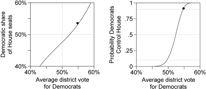
In this article we document this partisan bias, examine how and to what extent the Democrats overcame it, and offer predictions as to whether the results of the 2006 election leveled the electoral playing field for 2008—or perhaps even tilted it in the Democrats' favor. Before the election, we predicted the seats-votes curve using a district-level model of elections to translate the average district vote for Democrats into the number of seats they would gain (or lose) in the House (Kastellec, Gelman, and Chandler 2006). This strategy allowed us to predict systematically the outcome in each district across a range of hypothetical swings in the average district vote from 2004 to 2006. Our prediction of the translation between votes and seats was largely on the mark: The Democrats earned 54.8% of the average district vote, which our model predicted would lead to them winning 53.1% of the seats, or 231—just two short of their actual total of 233.
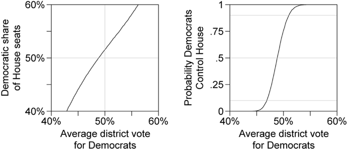
More generally, we found that in the range of plausible national election swings, the Democrats were always destined to receive fewer seats than their corresponding average vote share. They were able to gain control of the House by winning a commanding 54.8% of the average district vote, the largest margin for either party since 1990. Had their vote share been just 2% less, on average, a significant probability existed that the Republicans would have retained control of the House.
Did the Democrats' gain in 2006 eliminate the partisan bias in favor of the Republicans? Analysis of each party's vote share among their winning candidates suggests that the Republicans still hold a natural advantage in that their winning margins are smaller than the Democrats, meaning Republicans “waste” fewer votes. We use our model to make predictions about the 2008 elections, and find that the switch in incumbency advantage from the Republicans to the Democrats may nevertheless level the electoral playing field.
Predicting House Elections Nationally or by Districts
Forecasts of congressional elections typically focus on the production of a point prediction: the party out of power will pick up x seats, meaning they either will or will not control the House or Senate or both in the next Congress. The 2006 campaign witnessed no shortage of such predictions, with scholars basing their forecasts on such variables as presidential approval, economic conditions, and the generic congressional ballot (Abramowitz 2006; Bafumi, Erikson, and Wlezien 2007; Brandt and Brunell 2006; Campbell 2006; Cuzân and Bundrick 2006; Klarner and Buchanan 2006).2
The point predictions among these forecasts ranged from a low of Democrats winning 216 seats (Campbell 2006) to a high of them winning 235 seats (Bafumi, Erikson, and Wlezien 2007). The latter, which is similar to our approach in that the authors estimate a seats-vote curve based on the generic congressional ballot, came closest to the actual mark of 233.
Two exceptions are Bafumi, Erikson, and Wlezien (2007) and Klarner and Buchanan (2006), who incorporate both district-level and national-level information.
The use of macro-level variables to predict either the national vote or the seat division has a long lineage in the forecasting literature (see e.g., Tufte 1975; Lewis-Beck and Rice 1984; Oppenheimer, Stimson, and Waterman 1986; Marra and Ostrom 1989; Abramowitz, Cover, and Norpoth 1986; Erikson and Sigelman 1995; inter alia). And to be sure, macro-level predictions have their advantages. The point predictions that result from them are intuitive and lead to a dichotomous answer—which party will control the House—that is of interest to scholars, politicians, the media, and the public alike. It is also much easier to collect data at a single level of analysis per election, allowing one to ignore idiosyncrasies at the district level.
The district level, however, incorporates a wealth of information that macro-level predictions throw away by definition. Variables such as the predisposition of voters for one party or the other, incumbency, and whether a race is uncontested play crucial elements in determining the vote division in each race. This, in turn, determines who wins each race, which in turn affects the ultimate seat division. Thus, predicting the vote at the district level is true to the actual process by which seats are aggregated. It is also the only way to estimate a seats-votes curve for a single election. We employ this estimate to study the level of partisan bias that favored the Republicans in 2006 and how the Democrats overcame that bias.
Predicting the Seats-Votes Curve for a Single Election
We draw our prediction of the seats-votes curve in 2006 from a statistical model based on the framework for evaluating legislative elections advanced in Gelman and King (1994). The strength of this approach lies in its ability to forecast elections under a range of possible conditions through the use of simulation analysis that incorporates both a range of possible national swings and the predictive uncertainty inherent in any forecast. This incorporation of uncertainty allows us to make probabilistic predictions about the Democrats' chances of retaking the House. Finally, the approach is also quite parsimonious, employing as predictors only the vote in the prior election in each district, whether the incumbent is running for reelection, and whether the race is contested.
Simulating Election Outcomes under a Range of Hypothesized National Swings
Our method can be summarized informally as follows. (A formal description, along with details about variable coding, appears below.) We begin with the consideration that there is a range of possible national swings in the average district vote from one election year to the next. A swing in the direction of the Democratic party will help the Democrats pick up more seats; more specifically, every possible swing will have different implications in more closely contested elections and will lead to a different translation of seats for the Democrats. Our general strategy is to allow the swing to vary across a range of values, and then predict the outcome of every district at each interval in the range. Aggregating these results produces an estimated seats-votes curve.
The partisan swing, however, is unlikely to affect each district in the same manner. We account for district-level heterogeneity by incorporating incumbency and the district-level vote from the previous election, which serves as a proxy for the district's overall predisposition to support the Democratic candidate.4
For all analyses that appear in this article, we impute the district vote for uncontested races to 0.75 for Democratic winners and 0.25 for Republican winners. These values are derived in King and Gelman (1991) and Gelman and King (1994), based on the vote shares received in the last election before a district became uncontested and the first election after a district became uncontested. The average of these values was about 0.75 for the incumbent party and represents the average “effective support” for the party in uncontested races. For a measure based on the presidential vote in congressional districts, see Erikson (2006).
To account for uncertainty in the prediction, we simulate the outcome in each district 1,000 times, adding independent normally-distributed errors whose standard deviation is based on the residual error from historical House election forecasts. Finally, for each simulation, we shift the entire election result (that is, add or subtract a constant from all the districts) so that the average district vote matches up to that of the previous election. The result is 1,000 hypothetical election outcomes, each corresponding to a zero national swing (but various district-by-district differences). The next task is to add the national swing to each set of district-level results. We do so in the form of adding a constant to the predicted value within each simulation; we set the constant to a value that ensures that the range of national swings is centered around the average district vote from the previous election.
For every interval in the national swing (in the entire range of average district vote), we thus have 1,000 predicted outcomes in each congressional district. We summarize each simulation in two ways. First, we compute the average district vote; second, we compute the proportion of House seats won by the Democrats. Taking the mean seat proportion over all the simulations yields an expected seat share for the Democrats.5
Similar results are obtained by using the median instead of the mean to summarize predictive uncertainty.
Formally, we model the vote in each district as follows:

where v = the Democratic share of the two-party vote (as a number between 0 and 1), i indexes districts, t represents the current election (that in which the seats-votes curve is being predicted), and t-1 the previous election. The incumbency variable (defined in each district in each election year) is I = 1 if the incumbent in the district is a Democrat and seeking reelection, −1 if the incumbent is a Republican and seeking reelection, and 0 if the seat is open. For values of ψ (the estimated incumbency advantage), we use the trend of the values estimated in Gelman and Huang (forthcoming), who find a steadily increasing incumbency advantage from the 1940s to 1980, and a constant value of around 8% ever since.6
Specifically, we set ψ = 0.08((year-1946)/(1980–1946)) if year <1980, or ψ = 0.08 if year ≥ 1980.
We obtain values of ρ by regressing vit on vit−1, along with incumbency and party indicators, for each non-redistricting election year (i.e., those not ending in “2”) from 1946–2004. For each election year analyzed, we take the average of the coefficient on the lagged vote from the previous five years. The estimates of ρ have a mean of 0.68 with a standard deviation of 0.11.
We set σ to 0.066, which is the mean of the residual standard deviations from the yearly regressions discussed in the previous endnote.
For every value of δt, we simulate our model 1,000 times. For each simulation, we record the share of seats predicted to be won by Democratic candidates (that is,

, where n equals the number of districts in a given election year.
9In 1958 and 1960, respectively, 436 and 437 seats were contested due to the addition of Alaska and Hawaii as states. We also dropped the handful of races featuring third-party candidates (with the exception of Bernard Sanders—an independent who held Vermont's congressional seat from 1998–2004 and who organized with the Democratic party—whom we classified as a Democrat).
Validating by Fitting to Previous Elections
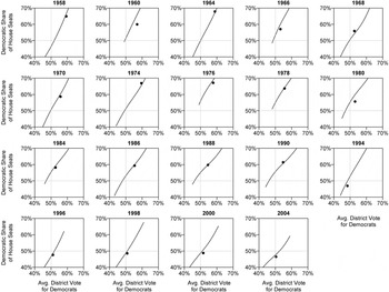
To demonstrate the validity of our method, we applied it to the 19 non-redistricting election years (i.e., those not ending in “2”) from 1958 to 2004. Figure 2 plots the predicted seats-votes curve for each year, along with the actual average district vote and seat share for the Democrats. The model performs fairly well, with a root mean-squared error of about 0.02, or about nine seats out of 435. Two elections (1960 and 1980) contribute disproportionately to the predictive error, as the model was off by 26 and 19 seats, respectively, in those years. For 10 of the elections, the prediction error was less than four seats. The root mean-squared error of the predictive standard deviation of seats given votes is 0.01, or about four seats, implying that the rest of the predictive error is due to year-to-year variation unexplained by the model. Thus, the model is not perfect, but we believe it demonstrates ample validity to serve as a useful tool for studying the relationship between seats and votes in the 2006 elections.

Seats-votes curve prediction and actual election results, 1958–2004 (excluding redistricting years)
Caption: For each year, the line depicts the estimated seats-votes curve, and the dot shows the actual election result. The light gray lines are references for 50% of the vote and 50% of the seats. As is well known (King and Gelman 1991), seats-votes curves have become less steep in recent decades—a given swing in votes will typically result in a lower swing in seats than before. As the plots show, the actual election result typically conforms closely to the predicted seats-votes curve.
Average District Vote and Total Vote
In this article we have summarized election results using the average district vote—that is, the parties' share of the two-party vote, averaged over the 435 congressional districts: for the Democrats, this is

. This is the usual way that political scientists aggregate congressional vote (King and Gelman 1991; Gelman and King 1994) and is a reasonable summary in that it is relatively immune to turnout variation and represents the national level of support for the party.
An alternative measure is the share of total vote that goes to the Democrats, which can be written as

, where Ti is the turnout (the number of votes for the two major parties) in district i. Total vote differs from average district vote because of district-by-district variation in turnout, which is correlated with the parties' vote shares.
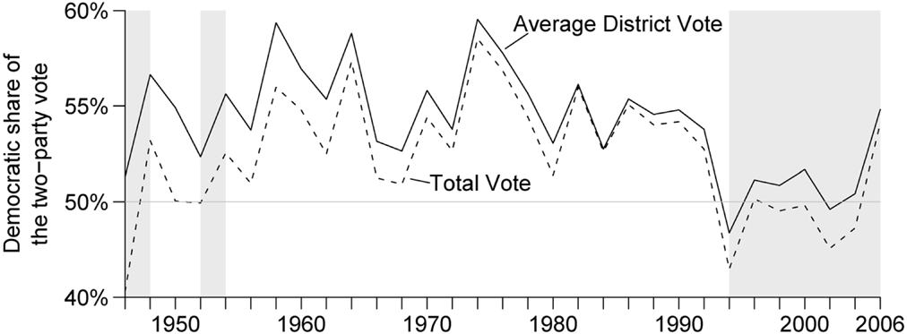
Figure 3 shows the time series of average district vote and total vote for the Democrats over the past 60 years. In the early period, the Democrats' average district vote was much higher than their total vote share, which can be attributed to their large number of uncontested, low-turnout districts in the South. In the past 15 years, a gap has again opened up, this time of about three percentage points, because the Democrats do better in low-turnout districts (for example, in inner cities). This trend continued in 2006: the Democrats won 54.8% of the average district vote, but only 53.3% of the total vote.

Democrats' share of the two-party total vote and average district vote in House elections, 1946–2006
Caption: Shaded areas represent periods of Republican control of the House.
As noted above, we prefer average district vote as a summary measure of national support for the parties, and so that is what we have used in this article.
Predicting and Dissecting the 2006 Seats-Vote Curve
Using this method, we predicted prior to the election the seats-votes curve for 2006, along with estimated probabilities of the Democrats taking control of the House given their average district vote.10
Information on incumbency status and retiring members was obtained from www.cq.com. Information on uncontested candidates was obtained from Giroux (2006)—candidates were considered uncontested if they were either a Democrat who did not face a Republican challenger or a Republican who did not face a Democratic challenger.
Vote totals for the Democratic and Republican candidates are based on official certified results from each state. As noted earlier, for each uncontested race, we imputed the vote to 0.25 for districts where no Democratic candidate ran and 0.75 for districts where no Republican candidate ran. Three districts warrant explanation. In Louisiana's 2nd district, where incumbent William Jefferson (D) won in a runoff election held in December 2006, we used the results of the original election to measure the Democrats' vote in the district because the runoff only featured Democratic candidates. In Texas' 23rd district, incumbent Henry Bonilla (R) was defeated in a December 2006 runoff. Here we used the results from the runoff election since it was contested by both parties. Finally, we used the official certified results from the election in Florida's 13th district, which was marred by apparent voting-machine malfunctions.
We generated predicted probabilities by taking the deterministic seats prediction (the expected value from a probabilistic district-by-district prediction) at each interval of the national swing and then adding predictive uncertainty based on the root mean-squared error of the historical seats-votes curves presented in Figure 2.

2006
Caption: (l) Predicted seats-votes curve for 2006; the point depicts the actual average district vote for Democrats (54.8%) and their share of House seats. Our point prediction was that they would win 231 seats (or 53.1% of seats) based on their average district vote of 54.8%, which turned out to be just two less than their actual total of 233 (53.6%) seats. (r) The predicted probability the Democrats would control the House given their average district vote. Light lines are references for 10%, 50%, and 90% probabilities. We estimate that the Democrats had a 90% probability of winning the House given the vote share they received.
Our model confirms that the Democrats faced a stacked electoral deck heading into the 2006 elections. They needed 52% of the average district vote just to have a 50% probability of winning the House, and needed nearly 55% (which they obtained) to ensure control. To borrow Krugman's (2006) metaphor, the Democrats needed a “storm surge” to overcome the “high Republican levee” erected by the Republicans' structural advantages.
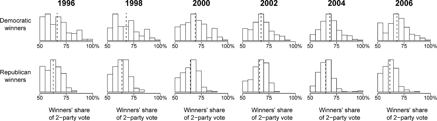
The source of the bias could be found largely in the difference between districts controlled by the two parties: some of this difference was due to geographic factors and favorable redistricting, and some to the Republicans' incumbency advantage. Figure 5 presents separate histograms of the vote shares for Democratic and Republican winners (excluding uncontested races) from each election from 1996 to 2006, along with the mean vote percentage for each. Consider first the five elections preceding 2006. In each year, the distribution of Democratic winner vote shares is more symmetric than that of Republicans, with a large percentage of Democratic winners earning more than 75% of the vote each year. In contrast, the distribution of Republican winner vote shares is much more skewed toward 50%, meaning they won their races by much smaller margins. In each year the mean Democratic winning vote share is also larger than the mean Republican winning vote share. Consider 2004: the Democrats won their victories with an average of 69% of the vote, while the Republicans averaged 65% in their contests, thus “wasting” fewer votes. The Republicans won 47 races with less than 60% of the vote; the Democrats only 28. Many Democrats are in districts where they win overwhelmingly, while many Republicans are winning the close races.

Distribution of vote margins for Democrats and Republicans in winning races, 1996–2006
Caption: For each year, the top histogram depicts the distribution of the Democratic share of the two-party vote in districts where Democrats won, while the bottom histogram gives the Republican share of the two-party vote in districts won by Republicans. The dotted lines represent mean vote shares. We exclude uncontested races to avoid clustering around 75%. For all years, the distribution of vote shares for Democratic winners is much more symmetric than for Republican winners, who are more skewed toward 50%. Likewise, the mean vote share for Democratic winners is systematically higher than that of Republican winners. In these years, Republicans “wasted” fewer votes, which contributed to the partisan bias against Democrats. This trend became even more pronounced in 2006.
So how did the Democrats' overcome the Republicans' advantages in 2006? In one sense, the answer is easy: they simply obtained a large enough share of the votes to guarantee control of the House. Their average district vote of 54.8% was thelargest since 1990, and three points higher than the 51.6% Republicans received in their landslide year of 1994. If the Democrats had received that same average district vote in 2006, according to our seats-votes curve the Democrats would have had only a 44% probability of winning the House. Thus, it took a large national swing for the Democrats to ensure their victory.
At the same time, the size of the Democrats' vote gain and seat gain obscures the structural disadvantages that prevented them from making even greater gains in 2006. For example, had the Republicans received 54.8% of the vote in 2006, we estimate they would have won about 249 seats, or 16 seats more than the Democrats obtained. Less obvious is that the incumbency advantage likely kept many Republicans in office. Of the 211 Republicans who ran for reelection, 189 won (or 90%); of those 211 winners, 47 (or 25%) earned less than 58% of the vote, meaning their victory can be attributed to the incumbency advantage (recall that the estimated average incumbency advantage is eight percentage points [Gelman and Huang forthcoming]). By contrast, all 191 Democratic incumbents who ran won; and only seven won by less than 58% of the vote. The last column in Figure 5 paints a more general picture, showing that in 2006 the Democratic victors continued their pattern of winning larger vote margins than their Republican winners. In fact, the difference between the mean vote shares of the two parties' winning candidates exceeded those of the previous five elections. And of the 118 races where the victor won with less than 60% of the vote, Republican candidates won 78 of them (or 66%).
Looking Ahead to 2008
It thus seems possible that the size of the Democratic victory hides a continuing structural disadvantage in House elections.13
The bias the Democrats face in the Senate is even more severe due to the Republicans' geographic advantage. As Hacker and Pierson (2006, 12) point out, “[a]ssuming senators represent half their states' residents, the 49 Democrats in the [110th] Senate represent approximately 40 million more Americans than the 49 Republicans.”
In each year since 1996, no fewer than 88% of House incumbents have run for reelection.
The results are presented in Figure 6. The results suggest that the Democrats' victory in 2006 did indeed remove the bias that favored the Republicans. Our model estimates that the Democrats will need just 49% of the vote to have a 50% probability of retaining control of the House, meaning the Republicans will need 51% to have an even chance of retaking it. Thus, while the Democrats may enjoy a partisan bias in 2008, it will likely be much less than the Republicans enjoyed in 2006. In addition, two other countervailing forces will affect the Republicans' chances in 2008. On the one hand, if our model is correct, the 51% of the average district vote they will need to have a 50% probability of retaking the House is larger than any percentage they have received since 1994. On the other, the Democrats will need to defend the seats of their first-term members who won in Republican-leaning districts in 2006, and are unlikely to receive as large an average vote share as they did in 2006. For this reason, the Democratic leadership gave these freshman favorable committee assignments in an effort to boost their incumbency advantage (Nagourney 2006).

2008
Caption: (l) Predicted seats-votes curve for 2008; (r) The predicted probability the Democrats will control the House given their average district vote. Light lines are references for 10%, 50%, and 90% probabilities.
Conclusion
We used a parsimonious model of elections to predict and analyze the translation between votes and seats in the 2006 House elections, and to make a preliminary assessment of the 2008 election. We validated the model on the previous half-century of House elections, as shown in Figure 2. As a methodological matter, it is crucial that we both took a district-level approach and estimated a separate seats-votes curve for each election, rather than combining several election results to estimate a time-averaged curve, as is often done. Our results show that it took a large wave of Democratic support in 2006 to overcome the Republicans' structural advantages, and that the Democrats' newfound incumbency advantage will help them in their efforts to retain control of the House in 2008, while by no means guaranteeing it.
Author Bios
Jonathan P. Kastellec is a Ph.D. candidate in the department of political science at Columbia University. He can be reached at: jpk2004@columbia.edu.
Andew Gelman is a professor in the departments of statistics and political science at Columbia University. He can be reached at: gelman@stat.columbia.edu.
Jamie P. Chandler is a graduate student in the department of political science at the City University of New York Graduate School and University Center, and a visiting scholar at the Institute for Social and Economic Research and Policy at Columbia University. Chandler can be reached at: jchandler@gc.cuny.edu.