NOMENCLATURE
- ADS
Air data sensors
- a x, a y, a z
linear acceleration components (m/sec2)
- EKF
Extended Kalman filter
- f, h
non-linear functions
- FDI
Fault detection and isolation
- g
gravitational acceleration (m/sec2)
- GPS
Global positioning system
- i
iteration index
- IMU
Inertial measurement unit
- INS
Inertial navigation system
- IOEKF
Iterated optimal extended Kalman filter
- j
sensor index
- k
time instant
- NSD
Navigation system data
- p, q, r
body rotational rate components (rad/sec)
- Q & R
process and Measurement noise covariance matrix
- RMSE
Root mean square error
- t
time (sec)
- U A, V A, W A
true airspeed velocity components (m/sec)
- Uc
control input
- U g
ground speed (m/sec)
- U gx, U gy, U gz
ground speed velocity components along x, y, z axis (m/sec)
- w & v
input and measurement noise vector
- V wN, V wE, W wD
wind velocity components in North-East-Down frame (m/sec)
- V t
true airspeed (m/sec)
- V w
wind velocity (m/sec)
- X & Z
state and measurement vector
- α
angle-of-attack (rad)
- β
angle of sideslip (rad)
- φ, ϑ, ψ
attitude angles (rad)
- σ & σ 2
standard deviation and variance
- ε Vt, α Vt, β Vt
errors of ADS state estimation
- ΔV t, Δα, Δα
sensor residuals
1.0 INTRODUCTION
Sensor fault detection plays a vital role in achieving efficient fault-tolerant control systems of aircraft. In the past few decades, many approaches were proposed for sensor fault detection and isolation(Reference Hajiyev and Caliskan1, Reference Berdjag, Zolghadri, Cieslak and Goupil2). In addition, the recent advancements were discussed in detail with various reconfiguring FDI approaches(Reference Inseok, Sungwan, Youdan and Chze Eng3–Reference Zolghadri5). An aircraft’s flight control system performance highly depends on the air data information measured by air data probes and is required to maintain safe flight. The air data (including airspeed, angle-of-attack, and angle of sideslip) sensor fault may occur due to various environmental anomalies that include icing in high altitudes, blockages in the Pitot-Static tube, ice formation in the rotating wind vanes, rainwater entry into the pressure ports, etc(6, Reference Lombaerts7). Since all the air data sensing mechanisms such as Pitot tubes and wind vanes are generally fitted outside the aircraft fuselage and can be affected by the same environmental variations, it may lead to multiple sensor failures. The failure of these sensors may cause damage to the aircraft and the passengers. There are some noticeable catastrophic failures recorded in the past due to air data sensor failures. Ice formation, because of water accumulation in the angle-of-attack (AoA) sensor during flight, resulted in a constant output on the AoA warning system(8). Similarly, the ice-clogged Pitot tubes caused incorrect airspeed indication to the pilot followed by loss of control of airplane(9). As discussed above, the air data sensor fault detection is important and requires reliable and accurate air data estimation. In order to maintain flight safety, the aircraft has to be equipped with a highly consistent fault-tolerant air data system. The fault detection of air data sensors (ADS) has been examined in several studies(Reference Rohloff, Catton and Whitmore10–Reference Castaldi, Mimmo and Simani13). In particular, the model-based FDI approaches have been considered as more practical for safety-critical systems such as aircraft. Some researchers used an aircraft model-based approach to estimate air data using an analytical redundancy approach, with longitudinal(Reference Freeman, Seiler and Balas14) and control surface modeling parameters(Reference Ganguli15). Other researchers proposed airspeed sensor fault detection of the unmanned aerial vehicle (UAV) with a statistical variation of the three different residual signals(Reference Hansen and Blanke16). However, all these methods depend on the accurate aircraft model. On the other hand, there is the redundant ADS fault detection without a specific aircraft model(Reference Van Eykeren and Chu17). However, this method relies on the output of redundant ADS which cannot be considered as a complete analytical redundancy approach. Recently, the data-driven-based air data sensor FDI was developed(Reference Fravolini, Delcore, Papa, Valigi and Napolitano18). The key advantage of this approach is that it is a model-free approach and has strong robustness. However, this method requires a rich quality of data to evaluate the fault detection algorithm. In recent times, the FDI approach with analytic redundancy without considering the aircraft model has noticeably increased; this means to keep away from the system uncertainties and complex dynamic equations. In addition, these approaches received greater attention among the research community because it does not require additional hardware, which places a need for future aircraft structural design optimisation requirements. Goupil et al.(Reference Goupil, Bauxell, Marcos, Cortet, Kerr and Costa19) presented the importance of mathematically developing redundancy (analytical redundancy) of flight parameters for reconfigurable fault-tolerant control systems. Recently, Lie and Egziabher(Reference Lie and Egziabher20) proposed the synthetic air data estimates to provide analytic redundant air data using Global Positioning System (GPS) and IMU information. More recently, some researchers proposed the Extended Kalman Filter- (EKF) based airflow angle and wind speed estimation with the aid of integrated Inertial Navigation System (INS) and GPS information(Reference Cho, Kang, Park and Yoo21).
With these newly developed approaches, it is noticed that the air data estimation and ADS fault detection are quite challenging where physical air data sensor measurements are not considered for air data estimation process. Furthermore, it is a much-needed solution to overcome all the past failures caused by the externally fitted air data probes. Since the performance of an FDI algorithm highly depends on the estimation algorithm, the non-linear estimators are preferable among other approaches. Most recently, an air data estimation method was proposed using the navigation system and flight control system information(Reference Lu, Li, Liu and Lei22). This has proved the validity of using onboard INS/GPS navigation system data to estimate air data parameters without considering the conventional air data probe-based air data measurements. However, this approach is more suitable for specific aircraft with an accurate dynamic model and may be affected by disturbances caused by environmental anomalies. Moreover, the normal EKF will suffer when system non-linearity increases, which may affect the accuracy of the estimation. Some researchers have proposed the EKF-based analytical method of aircraft sensor fault detection(Reference Ansari and Bernstein23, Reference D'amato, Mattei, Notaro and Scordamaglia24). However, these methods require complex calculations, which may increase computation time.
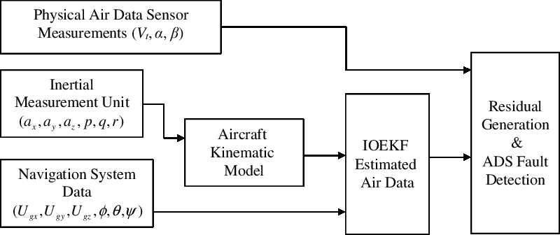
In this paper, a simple and reliable analytical redundancy-based Air Data Sensor Fault Detection (ADS-FD) approach is proposed using aircraft kinematics and onboard sensors information available on most of the modern aircraft. The proposed method utilises the IMU measurements and onboard navigation system data (NSD) such as ground speed and Euler (attitude) angles data to estimate the air data. Unlike the traditional air data estimation using redundant ADS, this approach does not consider the physical air data measurements to provide sensor fault detection. The key advantage of the proposed method is that it does not consider the specific aircraft model and can be applied to any aircraft. More specifically, it does not consider the system dynamics and considers only the sensor dynamics. In addition, it uses the aircraft equations of motion to build a simplified mathematical model that excludes the effect of aerodynamic forces (X, Y, Z) and moments (L, M, N) acting on the aircraft. Since these dynamic parameters are eliminated, the proposed method has less tuning complexity and free from model mismatches. With this knowledge, the airspeed, angle-of-attack, sideslip angle, attitude angles as well as the wind velocity are considered as a state vector, and the state equation is derived. Note that the estimation of attitude angle is important for accurate and reliable air data estimation. The estimated air data is compared with the physical ADS outputs which are not used in the filtering process. In order to implement this approach, the estimation under the variable wind field is considered for accurate air data estimation and to detect ADS fault. However, the unvarying wind field can also be considered under specific flight conditions. Note that, the wind speed information is necessary to properly relate the estimated air data using the proposed algorithm to physically measured air data. Considering the wind speed as an important factor, the IOEKF(Reference Havlík and Straka25) is chosen to estimate air data. Unlike normal EKF, an IOEKF eliminates the initial filtering error with good tracking performance and provides the best estimate. Based on the previous study, it is proved that the iterated version of EKF has better optimisation and tracking performance under various disturbances(Reference Zhao, Netto and Mili26). The key advantage of using the IOEKF is that it can track wind variation which is considered as unpredictable and unknown input in this approach. Therefore, an air data probes independent estimation including true airspeed, angle-of-attack and sideslip is presented using IOEKF. The estimated air data is used to detect ADS faults using the filter (IOEKF) generated residual signals. The fault detection (FD) scheme for the proposed method is shown in Fig. 1. As can be seen, FD using residual signal is reliable for model-based fault detection which carries only the fault information of the sensors and is not affected by system uncertainties. Moreover, the residual signals are easy to implement with simple equations to identify the type of sensor fault quickly. The proposed air data sensor fault detection algorithm is simulated using MATLAB software with simulated flight data from X-Plane flight simulator and validated using the real flight sensor data obtained from Cessna Citation II aircraft.
ADS fault detection scheme.

The contributions of this paper are: (1) an analytical redundancy-based air data estimation considering wind speed as the contributing factor is developed. The method only uses the input of IMU and the output of the integrated INS/GPS navigation system data. (2) The simplified aircraft model is considered to develop a mathematical model. The proposed model is estimated using IOEKF and the results show that the proposed method can detect sensor faults with good numerical accuracy. (3) Simulations are carried out using simulated flight data and real-time flight data. The fault detection of blocked air data probes (ADS) done and the results are analysed.
This paper is organised as follows. Section 2 describes air data modeling with the navigation system and the kinematic model. The relationship between the kinematic model and air data is illustrated first. Then, the mathematical connections among air data, ground speed and wind speed are established. The observability analysis and air data estimation framework are derived in Section 3. The fault detection algorithm is presented in Section 4 and the simulation results are discussed in Section 5. Concluding remarks are presented in Section 6.
2.0 AIR DATA MODELLING WITH AIRCRAFT KINEMATICS
To develop the ADS-FD method for aircraft air data sensors, the kinematic model with the IMU and the aircraft NSD is necessary. According to the aircraft kinematics principle, the equations of motion can be customised by eliminating the forces and moments as well as the mass (m) of aircraft in which the specific aerodynamic forces (in the centre of gravity) and angular rates measured by IMU serves as inputs(Reference Mulder, Chu, Sridhar, Breeman and Laban27). With the control instructions given, the aircraft’s kinematic model can generate the position, velocity, and attitude. The kinematics of aircraft is broadly studied and considered for this work. As can be noticed, using the relationship between air data and available measurements from IMU and NSD simple mathematical model can be created.
2.1 Determination of air data components
In this section, the air data to be estimated is represented using the wind velocity triangle relationship. The relationship between ground speed
 $(\skew5\vec{\it{\bf{U}}}_{g})$
, true airspeed
 $(\skew5\vec{\it{\bf{V}}}_{t})$
, and wind speed
 $(\skew5\vec{\it{\bf{V}}}_{w})$
of the aircraft relative to North-East-Down (NED) frame can be represented as,
 \begin{equation}{\skew5\vec U_g} = {\skew5\vec V_t} + {\skew5\vec V_w}\ldots\end{equation}
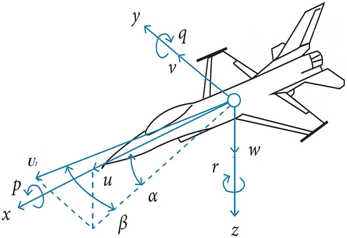
According to the relationship between aircraft body frame and wind frame components depicted in Fig. 2, the air data system parameters such as angle-of-attack/incidence (α), sideslip incidence / sideslip angle (β), and true airspeed
$(\skew5\vec{\it{\bf{V}}}_{t})$
measurable by air data probes are used to determine the true airspeed in the aircraft body frame:
 \begin{align}\begin{cases}{U_A} = {V_t}\cos \alpha \cos \beta\\{V_A} = {V_t}\sin \beta\\{W_A} = {V_t}\sin \alpha \cos \beta\end{cases}\ldots\label{eqn2}\end{align}
where (U A, V A, W A) are true airspeed velocity components represented as forward velocity, sideslip velocity, and vertical velocity, respectively. On the other hand, air data parameters can be calculated with the body-axes true airspeed components, which can be written as,
 \begin{align}\begin{cases}{V_t} = \sqrt {U_A^2 + V_A^2 + W_A^2}\\\alpha = {\tan ^{ - 1}}({W_A}/{U_A})\\\beta = {\sin ^{ - 1}}({V_A}/{V_t})\end{cases}\ldots\label{eqn3}\end{align}
Relationship between airspeed, angle-of-attack, and angle of sideslip.

In another perspective, the true airspeed using ground speed and wind speed can be defined as follows:
 \begin{equation}{V_t} = {\bf{R}}_{n}^b({U_g}) - {\bf{R}}_{n}^{b}({V_w})\label{eqn4}\end{equation}
Rewriting Equation (1) into the aircraft body-fixed reference frame, we have
 \begin{align}\left[\begin{array}{cccc}{U_{gx}}\\{U_{gy}}\\{U_{gz}}\end{array}\right] = \left[\begin{array}{cccc}{U_A}\\{V_A}\\{W_A}\end{array}\right] + {\bf{ R}}_{n}^b\left[\begin{array}{cccc}{V_{wN}}\\{V_{wE}}\\{V_{wD}}\end{array}\right]\label{eqn5}\end{align}
where (U gx, U gy, U gz) is the ground speed velocity components in the body frame,
 ${\bf{R}}_{n}^{b}$
is the rotation matrix from navigation to body frame, and (V wN, V wE, V wD) are NED components of wind speed. The above Equation (5) is true when wind variation is considered. However, during constant wind condition of flight, the time derivative of wind speed is equal to zero. Hence, the wind speed under constant wind condition can be determined as,
 \begin{equation}{\dot{\kern-2pt V}_w} = {\dot{\kern-2pt V}_{wN}} = {\dot{\kern-2pt V}_{wE}} = {\dot{\kern-2pt V}_{wD}} = 0\end{equation}
2.2 Derivation of aircraft kinematics model
Based on the aircraft kinematics principle, the motion of aircraft can be derived using the kinematic model without considering the aerodynamic forces and moments. The kinematic relations of aircraft is composed of positions (x, y, z), velocities (u, v, w), and attitude angles (φ, θ, ψ). From the measured accelerations and angular velocities, the linear velocity components and attitude of the aircraft can be obtained.
The time derivative of aircraft velocity can be written as,
 \begin{equation}\dot{\kern-2pt V} = a + {\bf{R}}_{b}^e{\bf{g}} - \omega \times V\end{equation}
where V is the airspeed along the body-axis, ‘a’ is the linear accelerations (a x, a y a z) along the body-axes,
 ${\bf{R}}_{b}^{e}$
is the rotation matrix from the body to earth frame, ‘g’ is the gravitational acceleration, and ‘ω’ is the angular velocities/rates (p, q, r) along the body-axes. In general, the aircraft acceleration
 $\underline{a}$
being produced by the vector sum of external forces acting on the aircraft, namely, the propulsive thrust
 ${(\underline{T})}$
, lift
 ${(\underline{L})}$
, drag
 ${(\underline{D})}$
, and the gravitational force acting on the aircraft mass (m)(Reference Collinson28).
Hence the following equations hold the true,
 \begin{equation}\underline{T} + \underline{L} + \underline{D} + m\underline{g} = m\underline{a} \label{eqn8}\end{equation}
and
 \begin{equation}\underline{a} = \frac{\underline{T}+ \underline{L} + \underline{D}}{m} + \underline{g}\label{eqn9}\end{equation}
where
 ${(\underline{T} + \underline{L} + \underline{D})/m}$
is the specific force. An aircraft’s accelerometer output along the forward axis (x), sideslip axis (y), and vertical axis (z) are denoted by a x, a y, a z respectively.
The typical aircraft accelerometer outputs in the three axes of aircraft body frame can be written as,
 \begin{equation}\begin{cases}{a_x} = \dot{\kern-2pt U} - Vr + Wq - g\sin \theta\\{a_y} = \dot{\kern-2pt V} + Ur - Wp + g\cos \theta \sin \phi\\{a_z} = \dot W - Uq + Vp + g\cos \theta \cos \phi\end{cases}\label{eqn10}\end{equation}
From Equations (7) and (10), it is shown that the measured accelerations can be used to determine the aircraft velocities. The aircraft velocity dynamics can be obtained by using Equation (10),
 \begin{equation}\begin{cases}\dot{\kern-2pt U} = {a_x} + Vr - Wq - g\sin \theta\\\dot{\kern-2pt V} = {a_y} - Ur + Wp + g\cos \theta \sin \phi\\\dot W = {a_z} + Uq - Vp + g\cos \theta \cos \phi \end{cases}\label{eqn11}\end{equation}
where (U, V, W) are the linear velocity components represented in the aircraft body-frame, and the attitude angle dynamics can be obtained by using the following equations,
 \begin{equation}\begin{cases}\dot \phi = p + q\sin \phi \tan \theta + r\cos \phi \tan \theta\\\dot \theta = q\cos \phi - r\sin \phi\\\dot \psi = q\sin \phi \sec \theta + r\cos \phi \sec \theta\end{cases}\label{eqn12}\end{equation}
where φ, θ, ψ are the Euler attitude angles. The above Equations (11) and (12) are the required aircraft kinematic model for the ADS fault detection in this paper. Equation (11) can be considered with constant wind condition; however, it is tenable for a short period of time. Taking changing wind variation into consideration, the performance of ADS-FD can be improved with accurate information. Hence, the following model is derived using the aircraft rigid-body kinematics principle:
 \begin{equation}\left[\begin{array}{cccc}{{\dot {\kern-2pt U}}_{gx}}\\[3pt]{{\dot {\kern-2pt U}}_{gy}}\\[3pt]{{\dot {\kern-2pt U}}_{gz}}\end{array}\right] = \left[\begin{array}{cccc}{a_x}\\[3pt]{a_y}\\[3pt]{a_z}\end{array}\right] + \left[\begin{array}{cccc}{U_{gx}}\\[3pt]{U_{gy}}\\[3pt]{U_{gz}}\end{array}\right]\left[\begin{array}{cccc}0 & r & - q\\[3pt]- r & 0 & p\\[3pt]q & -p & 0\end{array}\right] + \left[\begin{array}{cccc}-\sin \theta \\[3pt]\cos \theta \sin \phi\\[3pt]\cos \theta \cos \phi\end{array}\right] g\label{eqn13}\end{equation}
From Equations (10) to (12), the relationship of air data, navigation system, inertial accelerations (a x, a y, a z), and angular velocities is determined. Based on this kinematic model, the linear accelerations and angular velocities (p, q, r) from IMU become control information and the ground speeds (U gx, U gy, U gz) and attitude angles (φ, θ, ψ) from NSD are considered as measurement information and as functions of air data (V t, α, β).
3.0 AIR DATA ESTIMATION METHODOLOGY
In this section, a simple and reliable air data estimation method is presented combining the IMU, NSD, and aircraft kinematics. The air data mathematical model used for filtering in this paper differs from that of Lu (2018)(Reference Lu, Li, Liu and Lei22), which used rotational rates as states, and attitude angles from the NSD as measurements. In this method, the rotational rates and linear accelerations considered as inputs and NSD-calculated ground velocities and attitude angles are considered as measurements. The linear accelerations and rotational rates have a direct relationship with the airspeed and attitude of the aircraft, respectively. With a change in attitude of the aircraft, the attitude variations computed by the INS is used to estimate attitude angles. Hence the accurate and stable output of NSD provided attitude information is preferred. Note that the accurate position and Euler attitude angle information is necessary for the accurate air data estimation, which can be provided by the aircraft navigation system calculations. In order to obtain the above information, the air data, attitude angle, and wind speed are considered as states to be estimated for the proposed FD in this paper.
3.1 Determination of system state and measurement equations
With the aircraft kinematics model, the non-linear state-space model of the system is formulated as,
 \begin{equation}{\dot{\bf{X}}} = f({\bf{X}},{{\bf{U}}_c}) + {\bf{w}}\label{eqn14}\\[-28pt]\nonumber\end{equation}
 \begin{equation}{\bf{Z}} = h({\bf{X}}) + {\bf{v}}\label{eqn15}\end{equation}
where X represents the state vector, Uc represents the controllable input vector, and Z is the measurement vector. The functions f and h are non-linear functions. The variables of the system equations are described as follows:
 \begin{equation}{\bf{X}}={[{V_t}\ \alpha \ \beta \ \phi \ \theta \ \psi \ {V_{wN}}\ {V_{wE}}\ {V_{wD}}]^T}\label{eqn16}\\[-25pt]\nonumber\end{equation}
 \begin{equation}{{\bf{U}}_c} = {[{a_x}\ {a_y}\ {a_z}\ p\ q\ r]^T} + {\bf{w}}\label{eqn17}\\[-25pt]\nonumber\end{equation}
 \begin{equation}{\bf{Z }}={[{U_{gx}}\ {U_{gy}}\ {U_{gz}}\ \phi \ \theta \ \psi ]^T}\,{+}\, {\bf{v}}\label{eqn18}\nonumber\end{equation}
where system state vector (X) represents the system parameters including true airspeed, angle-of-attack, angle of sideslip, Euler or attitude angles and north-east-down wind velocity components; input vector (U c ) represents the IMU measurement, which measures the linear accelerations (a x, a y, a z) along three body-axes and rotational rates (p, q, r) along three body-axes; the measurement vector (Z) represents the measured output from the INS/GPS navigation system including ground speed velocity components in the body frame and Euler angles; w is the input noise, which is the zero-mean Gaussian process noise, with covariance matrix Q and v is the zero-mean Gaussian measurement noise vector, with covariance matrix R. The state update for the Euler angles and wind speed can be obtained using Equations(12) and (6). The state update equations for the air data variables (V t, α, β) can be obtained by differentiating Equation (2) as
 \begin{equation}\left[\begin{array}{ccc}\dot{\kern-2pt V}\\[3pt]{\dot \alpha }\\[3pt]{\dot \beta }\end{array}\right] = \left[\begin{array}{c@{\quad}c@{\quad}c}\cos \alpha \cos \beta &{\rm{ sin}}\beta \ &\sin \alpha \cos \beta\\[4pt]\dfrac{{ - \sin \alpha }}{{{V_t}\cos \beta }}& {\rm{ 0 }} &\dfrac{{\cos \alpha }}{{{V_t}\cos \beta }}\\[12pt]\dfrac{{ - \cos \alpha\, {\rm{sin}}\,\beta }}{{{V_t}}}& \dfrac{{\cos \beta }}{{{V_t}}}& \dfrac{{ - \sin \alpha \sin \beta }}{{{V_t}}}\end{array}\right]\left[\begin{array}{ccc}{{\dot {\kern-2pt U}}_A}\\[3pt]{\dot{\kern-2pt V}_A}\\[3pt]{{\dot W}_A}\end{array}\right]\label{eqn19}\end{equation}
where
 ${({\dot{\kern-2pt U}_A},{\dot{\kern-2pt V}_A},{\dot W_A})}$
can be calculated using Equations (5) and (6), which can be presented as
 \begin{equation}\left[\begin{array}{cccc}{{\dot {\kern-2pt U}}_A}\\[3pt]{\dot{\kern-2pt V}_A}\\[3pt]{{\dot W}_A}\end{array}\right] = \left[\begin{array}{cccc}{{\dot {\kern-2pt U}}_{gx}}\\[3pt]{\dot{\kern-2pt V}_{gy}}\\[3pt]{{\dot W}_{gz}}\end{array}\right] + \left[\begin{array}{cccc}0 & r & -q\\[3pt]-r & 0 & p\\[3pt]q & -p & 0\end{array}\right]\left[\begin{array}{cccc}{V_{wN}}\\[3pt]{V_{wE}}\\[3pt]{V_{wD}}\end{array}\right]\label{eqn20}\end{equation}
where
${({\dot{\kern-2pt U}_A},{\dot{\kern-2pt V}_A},{\dot W_A})}$
described in Equation (20) is the velocity state dynamics including wind velocity state dynamics considered in the body frame. Due to the arbitrary nature of wind, for example, turbulence, it is difficult to achieve the prediction of local wind field variation. In general, the wind velocities with turbulence are considered as random variables. Hence, the state dynamics of wind velocity is represented as a stochastic process model and it is givenby,
 \begin{equation}{\dot{\kern-2pt V}_w} = {\left[ {{V_{wN}}\ {V_{wE}}\ {V_{wD}}} \right]^T} = {{\bf{w}}^{{V_w}}}\label{eqn21}\end{equation}
where (V wN, V wE, V wD) are the wind velocity components represented in the NED frame and wVw is the stochastic process noise considered for wind velocity estimation. Therefore, the process noise vector represented in Equation (17) is determined with three components of accelerations, rotational rates, and wind velocity, which are presented as follows:
 \begin{equation}{\bf{w}} = \left[\begin{array}{cccc}{w^a}\\[3pt]{w^\omega }\\[3pt]{w^{{V_w}}}\end{array}\right]\label{eqn22}\end{equation}
where w a and w ω are the input noise components from IMU i.e. accelerometers and rate gyros.
In this paper, it is assumed that there are no faults in the GPS and IMU sensors. If there are faults in the GPS and IMU, they can be detected using a different set of kinematic model and information from other sensor measurements.
3.2 Estimation framework of iterated optimal extended Kalman filter
The proposed model contains non-linearity and requires a non-linear estimator. Therefore, a non-linear filter such as IOEKF is used to estimate the states of the system and to detect sensor faults. Considering the nonlinear character of the measurement equations, the IOEKF is applied to the state estimation problem of the model described by Equations (14) and (15). In general, the nature of the EKF(Reference Julier and Uhlmann29) is minimum variance estimation following linearisation and discretisation for a nonlinear system through first-order Taylor approximation. For the proposed method, the discrete time state-space model is considered with additive noise as follows:
 \begin{align}\begin{cases}{{\bf{X}}_k} = f({{\bf{X}}_{(k - 1)}},{{\bf{U}}_c}_{(k - 1)},{{\bf{w}}_{(k - 1)}})\\[3pt]{{\bf{Z}}_k} = h({{\bf{X}}_k}) + {{\bf{v}}_k}\end{cases}\label{eqn23}\end{align}
where Xk ဓ Rn is the state of the system at discrete time step k; Zk ဓ Rm is the measurement;
 ${{\bf{w}}_{k - 1}}\sim N(0,\ {\bf Q}) $
and
 ${{\bf{v}}_k} \sim N(0,\ {\bf R})$
are the system random noise and random measurement noises which are considered to be unrelated, Gauss white noises with zero-means of Qk-1 and Rk respectively.
The idea of the IOEKF is to improve a reference trajectory, and consequently the estimate, in the presence of significant nonlinearities. Those improvements are achieved by local iterations of the EKF measurement update. The iterations are usually stopped when there is no significant change in consecutive iterations or other criteria such as a maximum number of iterations are met. Hence, the filter equations from normal EKF are used to frame the IOEKF are as follows:
Step 1: Initialisation
 \begin{align}\begin{cases}{\hat{\bf X}}_0 = E({\bf{X}}_0)\\[4pt]{\bf{P}}_0 = E(({\bf{X}}_0 - {\hat{\bf X}}_0)\,({\bf{X}}_0 - {\hat{\bf X}}_0)^{T})\end{cases}\label{eqn24}\end{align}
where X0 and P0 are initial state and initial error covariance matrix, respectively.
 ${\hat{\bf X}}_0$
is the estimated initial state; k is the time;
 ${\hat{\bf X}}$
is the state estimation; Pk is the error covariance; Kk is the Kalman gain.
Step 2: Time update
 \begin{align}\begin{cases}{\hat{\bf X}}_{k + 1| k } = {f_k}({\hat{\bf X}}_{k| k})\\[4pt]{{\bf{P}}_{k + 1| k }} = {{\bf{F}}_k}{{\bf{P}}_{k| k }}{\bf{F}}_k^T + \sum {_k^{\bf{w}}} \end{cases}\label{eqn25}\end{align}
Step 3: Measurement update
 \begin{align}{\hat{\bf X}}_{k| k } & = {\hat{\bf X}}_{k| k - 1} + {\bf{K}}_k({\bf{Z}}_k - {\bf{h}}_k({\hat{\bf X}}_{k| k - 1}))\nonumber\\[4pt]{\bf{P}}_{k| k } & = {\bf{P}}_{k| k - 1} - {\bf{K}}_k{\bf{H}}_k{\bf{P}}_{k| k - 1}\label{eqn26}\end{align}
where
 ${{\bf{K}}_k} = {{\bf{P}}_{k| k - 1}} - {\bf{H}}_k^T{{\bf{(}}{{\bf{H}}_k}{{\bf{P}}_{k| k - 1}}{\bf{H}}_k^T + \sum {_k^{\bf{v}}} )^{ - 1}}$
is the Kalman gain.
In order to implement the IOEKF, set the predictive estimate
 ${\hat{\bf X}}_k^i = {{\hat{\bf X}}_{k\left| {k - 1} \right.}}$
and set the iteration i = 0. Therefore, the Jacobi matrix computed at the best state estimate available along with the Kalman gain and the next iteration of state estimate,
 ${\bf{H}}_k^i$
which is presented as follows:
 \begin{equation*}{\bf{H}}_k^i = {\left. {\frac{{\partial {{\bf{h}}_k}(s)}}{{\partial (s)}}} \right|_{s = {\hat{\bf X}}_k^i}}\end{equation*}
Hence the measurement update equations are presented with the above information as follows:
 \begin{align}{\bf{H}}_k^i & = {\left. {\frac{{\partial {{\bf{h}}_k}(s)}}{{\partial (s)}}} \right|_{s = {\hat{\bf X}}_k^i}}\nonumber\\[3pt]{\bf{K}}_k^i & = {{\bf{P}}_{k| k - 1}} - {[{\bf{H}}_k^i]^T}{\left({\bf{H}}_k^i{{\bf{P}}_{k| k - 1}}{[{\bf{H}}_k^i]^T} + \sum {_k^{\bf{v}}} \right)^{ - 1}}\nonumber\\[3pt]{\hat{\bf X}}_k^{i + 1} & = {{\hat{\bf X}}_{k| k - 1}} + {\bf{K}}_k^i({{\bf{Z}}_k} - {{\bf{h}}_k}({\hat{\bf X}}_k^i) - {\bf{H}}_k^i({{{\hat{\bf X}}}_{k| k - 1}} - {\hat{\bf X}}_k^i))\label{eqn27}\end{align}
Repeat the above steps with i = i + 1 until a stopping criterion is met. Now save the last iteration as the new filtering mean, and compute the covariance matrix based on the last iteration,i.e.,
 \begin{align}\begin{cases}{{{\hat{\bf X}}}_{k| k }} = {\hat{\bf X}}_k^i\\[3pt]{{\bf{P}}_{k| k }} = ({\bf{I}} - {\bf{K}}_k^i{\bf{H}}_k^i){{\bf{P}}_{k| k - 1}}\end{cases}\label{eqn28}\end{align}
Hence, the above equations show that the filter is optimum to estimate air data parameters. The results comparing the estimation performance of EKF (non-iterated) and IOEKF is presented in Section 5.1.
3.2.1 Computational complexity of IOEKF
In general, the EKF is preferred for nonlinear systems approximation whose computational load related to the cube of the state vector dimension (n)(Reference Daum30). The most intensive computational complexity of the EKF and IOEKF is determined as O(n 3). Since the computation of the IOEKF-based system considers the few iteration steps to estimate the state (whereas EKF does not do this iteration steps); it is reasonable for a mathematically intensive system. Therefore, it is straightforward to mention that the IOEKF has less computational complexity than a non-iterative EKF.
4.0 FAULT DETECTION ALGORITHM
This section discusses the fault detection of ADS using IOEKF-generated residual signals. The estimated states of the proposed system are used to generate the residual signal by comparing the physical measurements of ADS with filter estimated values. Note that the physical ADS measurements are not used in the filtering process and are just used as a comparison reference to detect ADS faults.
4.1 Residual generation
In general, residual (e) is defined as the difference between the true value of the dependent variable (z) and the estimated value
 ${(\hat{z})}$
. In analytical redundancy and model-based FD approaches, physical quantities that indicate variation due to the fault are called a residual signal. Assuming all other sensors are working properly, the following simple equation is used to determine the residual signal e(k):
 \begin{equation}e(k) = {z_k} - {\hat z_k}\label{eqn29}\end{equation}
Under normal operation of sensors, the residual should be close to zero. When a fault occurs, this signal should deviate from zero by exceeding a fixed threshold value. Under sensor faulty conditions, the estimated values
${(\hat{z})}$
will replace the failure ADS measurements to provide analytical redundancy, which is to ensure the safe operation of the system.
4.2 Residual evaluation
In order to determine the fault condition of the sensors, a suitable decision-making function is preferred. In one of the studies, the fixing of the threshold in the time and frequency domain is analysed(Reference Frank and Ding31). Faitakis et al.(Reference Faitakis, Thapliyal and Kantor32) studied the computation of thresholds using vector and matrix norm operations. Another researcher set an adaptive, positive, and negative threshold within a sliding time window(Reference Lu, Van Eykeren, Van Kampen, De Visser and Chu33). The residual signals obtained by the IOEKF are adequately stable, and a simple threshold to detect sensor fault can detect faults easily. The predetermined threshold can be written in simple equation form as
 \begin{equation}e_k^{\,j} = z_k^{\,j} - \hat z_k^{\,j}\end{equation}
where
 $e_{k}^{\,j}$
is the residual of the j
th
sensor at time, k when there are no faults;
 $z_{k}^{\,j}$
is the measured signal of the j
th
sensor, and
 $\hat{z}_{k}^{\,j}$
is the estimated value of the corresponding j th sensor.
The threshold test can be performed by comparing the generated residuals with its statistical values under normal condition. Thus, the decision-making function with a binary decision variable (δ r ) and with a fixed threshold is introduced as follows:
 \begin{align} \begin{cases}\left| {e_k^{\kern1.7pt j}} \right| \le {\mu _j} + {\sigma _j}\left| {e_k^{\kern1.7pt j}} \right|\quad {\rm{ for }}\ {{\rm{f}}_k} = 0 \Rightarrow {\delta _r} = 0\quad {\rm{ fault\ free\ condition}}\\[7pt]\left| {e_k^{\kern1.7pt j}} \right| > {\mu _j} + {\sigma _j}\left| {e_k^{\kern1.7pt j}} \right|\quad {\rm{ for }}\ {{\rm{f}}_k} \ne 0 \Rightarrow {\delta _r} = 1\quad {\rm{ faulty\ condition}}\end{cases}\label{eqn31}\end{align}
where μ
j
and
 $\sigma_{j}^{2}$
are the mean and variance of the j
th
sensor residual, respectively, under fault-free condition; f
k
is the fault vector which is also called as the alarm signal; When there is no fault, the alarm signal will be set to 0. If
 $\left|e^{\kern1.5pt j}_{k}\right|$
exceeds the predetermined value, we can conclude that a fault is expected and the alarm signal will be set to 1. The proposed fault detection process uses this logic to detect ADS faults.
5.0 RESULTS AND DISCUSSIONS
In this work, the fault of the air data sensors including airspeed, angle-of-attack, and angle of sideslip is presented using estimated air data. First, the estimation performance of IOEKF compared with EKF to guarantee the filter is optimum for the proposed method. Note that the estimation accuracy is necessary for the ADS-FD using IOEKF. For the proposed algorithm, the simulation results are obtained from MATLAB software. The sensor fault such as constant output fault is considered. In order to implement this, the process noise (Q) and measurement noise covariance (R) matrices are determined using the sensor specifications which are considered as constants in the filtering process.
5.1 Simulation results for comparison of EKF and IOEKF estimation
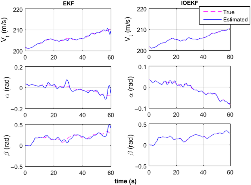
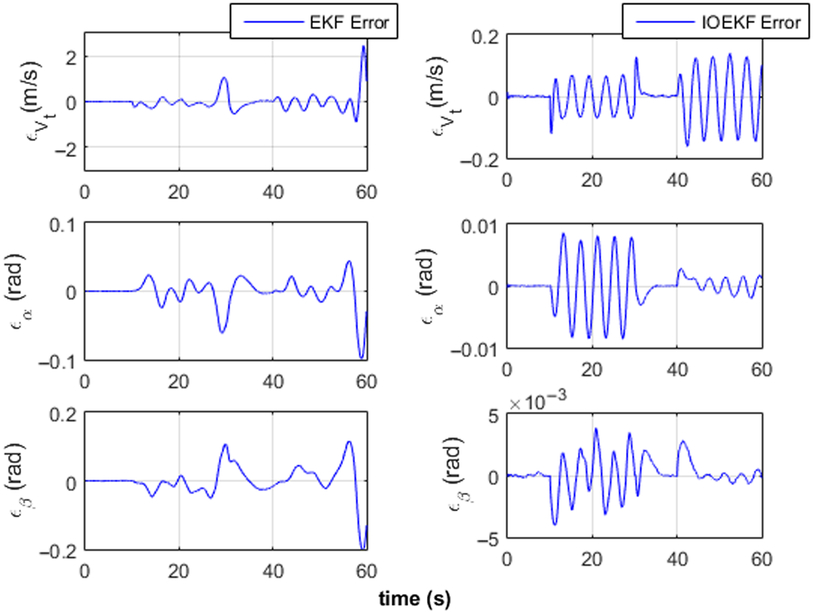
In this subsection, the simulation results comparing the performance of EKF and IOEKF state estimation is presented. Figures 3 and 4 show the comparison results of air data estimation and estimation error for airspeed (V t), angle-of-attack (α), and angle of sideslip (β).
EKF and IOEKF state estimation.

Error of state estimation.

As can be noticed, the performance of IOEKF is better than the EKF, which suffers due to its limitations in the presence of increased non-linearity. The estimation of IOEKF converges better than the EKF and the estimation error (∊ Vt, ∊ α, ∊ β) significantly reduced with IOEKF than the EKF. The root mean square error (RMSE) of the air data parameters using EKF and IOEKF are V t = 0.3861, α = 0.0216, β = 0.0460 and V t = 0.0638, α = 0.0033, β = 0.0013, respectively. As can be seen, the IOEKF is optimum for the proposed ADS-FD algorithm.
5.2 ADS-FD simulation results using flight simulator data
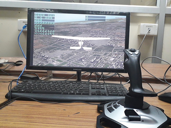
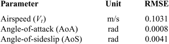
In this subsection, the simulation results using flight data obtained from X-Plane flight simulator under calm wind condition for a short time is presented. The simulated flight was conducted using X-Plane flight simulator version 10.0 with a USB joystick interface with the computer as shown in Fig. 5. The simulation was carried out with Cessna 172 aircraft with a predetermined dataset, which can be selected on the X-Plane window before each flight. The simulator generated flight data including various variables considered for the proposed mathematical model is used in the filtering process and the air data estimated for the ADS-FD. The update rate is selected as 100 Hz for the simulated data. The noise assumptions for the simulated flight data variables are given in Table 1. The captured flight log is used for the simulation of sensor FD by introducing faulty information into the flight data which is presented in Figs. 6 and 7.
X-Plane flight simulation setup.

Noise assumptions for the simulated flight data

Statistical characteristics of estimation using flight simulator data

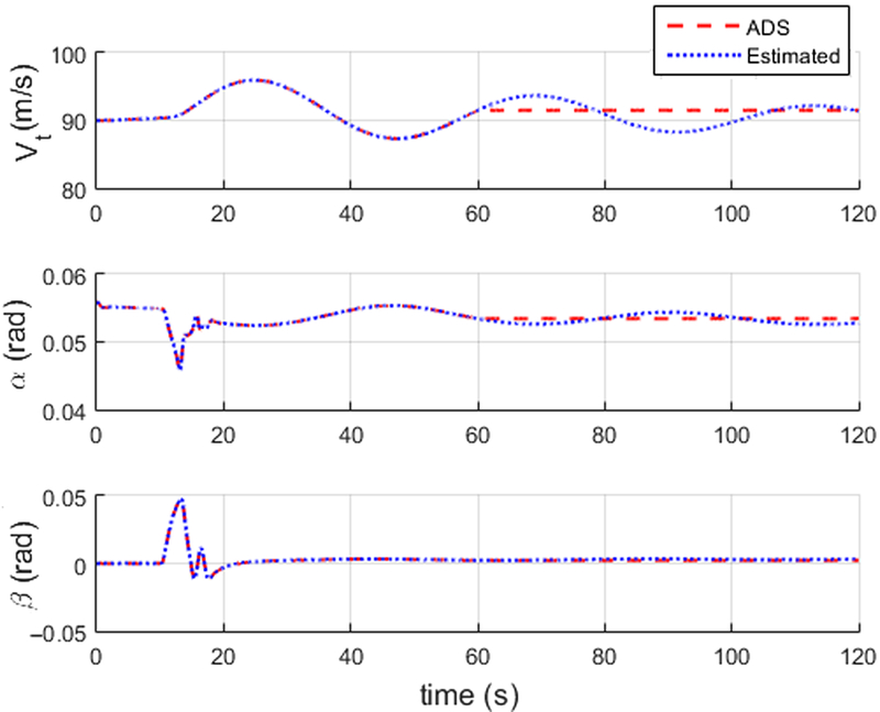
ADS constant output fault at t = 60sec.

The simulation results obtained from MATLAB software with constant output fault for the ADS including airspeed, angle-of-attack, and angle of sideslip are presented as follows:
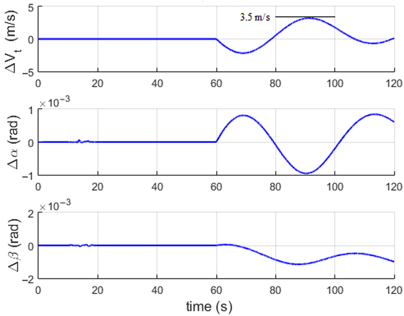
Figure 6 shows the simulation results of ADS with constant output fault. At t = 60sec, the fault is detected when the constant output fault occurs. The ADS residuals (ΔV t, Δα, Δα) shown in Fig. 7 vary significantly after the sensor fault. Before fault, the residuals are close to zero, which shows that the filter accuracy is sufficient to detect ADS faults. As it can be noticed, the airspeed residual after the fault reaches to a maximum value of 3.5m/sec; the angle-of-attack residual reaches to a maximum value of 1 × 10⁻³ rad; the angle of sideslip residual reaches to a maximum value of 1 × 10⁻³ rad. The statistical characteristics of the filter estimated parameters are listed in Table 2.
ADS residual variation after fault.

5.3 ADS-FD validation results using real-time flight data
In this subsection, the validation of ADS-FD under variable wind condition using real-time flight data obtained from Cessna Citation aircraft is presented. The flight data includes GPS, IMU (accelerometers and rate gyros) measurements considered for the estimation and FD of the proposed method. It also has the ADS measurements (airspeed, angle-of-attack, and angle of sideslip). Note that the ADS measurements are not used in the filtering process and used only for comparison reference with the estimated values. The specifications of sensors used on the Cessna Citation aircraft flight test listed in Table 3. The ADS-FD results using real-time flight data are presented below:
Sensors specifications used for the real-time flight data

To validate the proposed FD method, the constant output fault is introduced in the ADS measurements, which are not used in the filtering process. The constant output fault is considered to address the air data probe blockage fault which will lead to a constant output of the ADS. The simulation results obtained from MATLAB software are presented as follows:
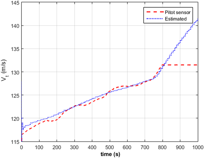
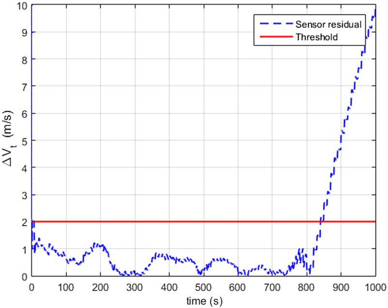
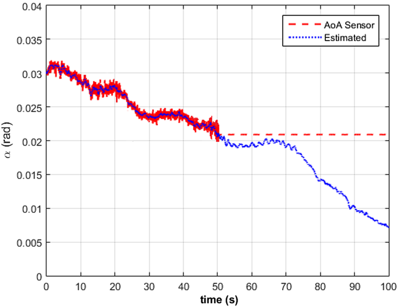
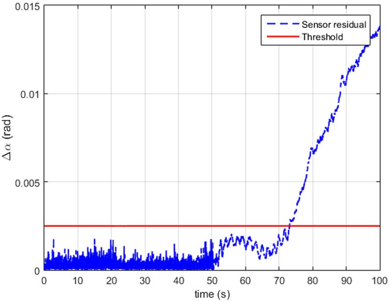
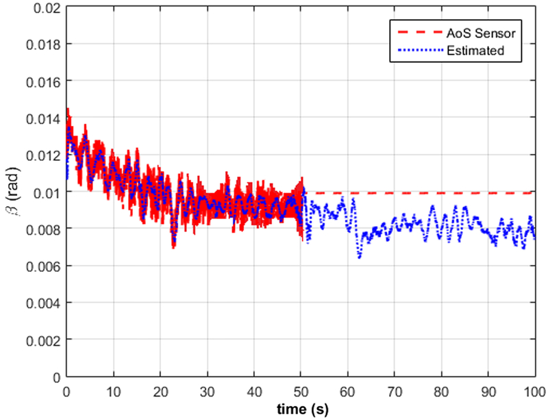
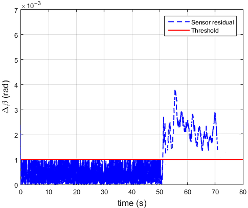
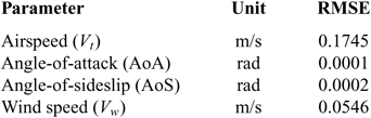
Figure 8 shows the airspeed sensor with constant output fault. At time t = 800 sec, airspeed sensor becomes faulty with constant output at the airspeed value of 131.6m/sec. However, the filter estimate can continuously provide air data. Figure 9 shows the residual variation after the airspeed sensor fault exceeds the predetermined value of 2m/sec and reaches to a maximum value of 9.85m/sec, and hence the fault is detected. The RMSE of airspeed is around 0.1745m/sec, which shows that the filter is accurate enough to detect airspeed sensor fault. Figure 10 shows that the constant output fault occurs in the AoA sensor at time t = 50sec and at AoA (α) = 0.021rad. Figure 11 shows the residual variation of the AoA sensor after fault, which exceeds the predetermined threshold of 0.002rad and reaches to a maximum value of 0.014rad. Figure 12 shows the AoS sensor constant output fault at time t = 50sec, AoS (α) = 0.01rad. Figure 13 shows AoS residual variation after the fault. The residual of the AoS sensor exceeds the predetermined value of 0.001rad after the constant output fault. The statistical characteristics of the estimated parameters are listed in Table 4.
Airspeed sensor constant output fault.

Airspeed residual after fault.

AoA sensor constant output fault.

AoA residual after fault.

AoS sensor constant output fault.

AoS residual after fault.

6.0 CONCLUSION
In this paper, we presented the air data probe independent analytical redundancy approach to fault detection of air data sensors. For the proposed method, we used the aircraft kinematic relations between different quantities. In order to implement the proposed algorithm, we introduced a constant output fault in the sensor measurements and simulated the same using MATLAB software. The iterated version of the optimal extended Kalman filter developed, and it appears to be sufficient for the proposed algorithm even when the nonlinearity of the system increases drastically. With the estimated states, the physically measured quantities from the air data probe are compared to detect sensor faults. The results show that the estimated data can be used to detect the air data sensor faults and to provide back-up air data measurements when a redundant sensor goes off.
The future work intends to accommodate the proposed analytical redundancy in UAVs where it would play a predominant role in terms of weight reduction. The proposed algorithm may be further validated through several flight tests with an experimental setup including a fixed-wing UAV, to show the effectiveness of the FD process.
Statistical characteristics of estimation using real-time data

ACKNOWLEDGEMENT
The authors would like to thank Peng Lu of The Hong Kong Polytechnic University for sharing the flight data of the Cessna Citation II aircraft.