1 Introduction
Rough-wall turbulent boundary layers are encountered in both nature and engineering (Raupach, Antonia & Rajagopalan Reference Raupach, Antonia and Rajagopalan1991; Barlow & Coceal Reference Barlow and Coceal2008; Bons Reference Bons2010). Modelling drag forces on rough walls is a research topic that has received sustained attention (Jiménez Reference Jiménez2004; Schultz & Flack Reference Schultz and Flack2009; Schlichting & Gersten Reference Schlichting and Gersten2016). Recently, with increasing use of additive manufactured parts in the turbomachinery industry, a new interest has emerged in modelling drag forces on 3D printed rough surfaces (see e.g. Ferster, Kirsch & Thole Reference Ferster, Kirsch and Thole2018; Kirsch & Thole Reference Kirsch and Thole2018).
A well-studied model problem for rough-wall turbulent boundary layers is flow over aligned and staggered cube arrays (see e.g. Coceal et al.
Reference Coceal, Thomas, Castro and Belcher2006; Cheng et al.
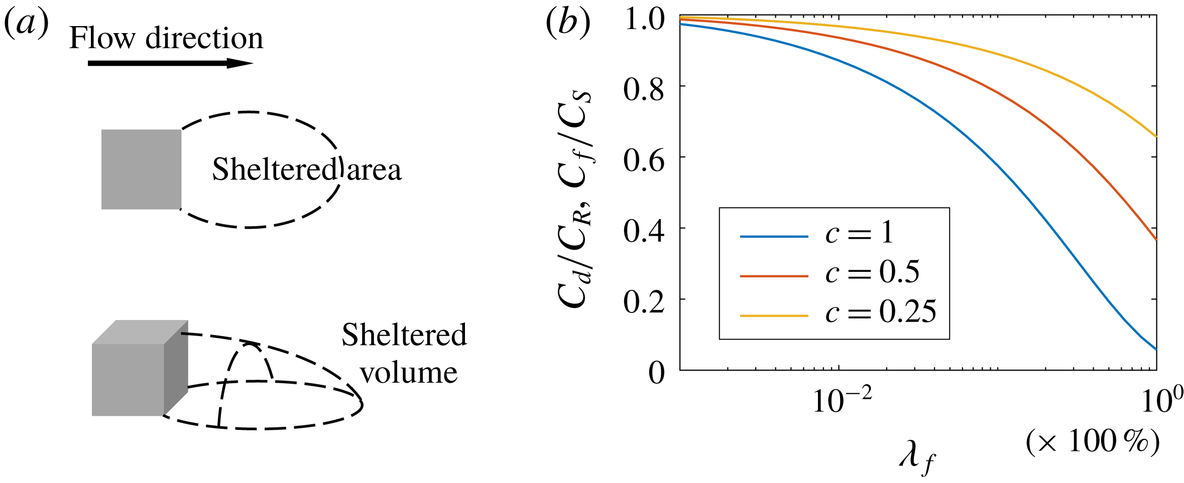
Reference Cheng, Hayden, Robins and Castro2007; Leonardi & Castro Reference Leonardi and Castro2010; Lee, Sung & Krogstad Reference Lee, Sung and Krogstad2011). Aside from empirical models (Moody Reference Moody1947; Taylor, Coleman & Hodge Reference Taylor, Coleman and Hodge1985), the theoretical work by Arya (Reference Arya1975) and Raupach (Reference Raupach1992) on drag partition lays the groundwork of rough-wall drag-force modelling. Raupach argues that a cubical roughness element ‘shelters’ its downstream ground area and volume (see figure 1
a). The sheltered ground area and the sheltered volume scale as
 $h^{2}U_{h}/u_{\unicode[STIX]{x1D70F}}$
and
 $h^{3}U_{h}/u_{\unicode[STIX]{x1D70F}}$
, respectively, where
 $h$
is the cube height,
 $U_{h}$
is the spatially and temporally averaged wind speed at the cube height, and
 $u_{\unicode[STIX]{x1D70F}}$
is the friction velocity. If a roughness element is not sheltered, it acts as an isolated element. Raupach (Reference Raupach1992) concludes that, at low surface coverage densities, the drag force on a rough surface increases linearly with the number of roughness elements (given an outer flow), and the single-cube drag coefficient,
 $$\begin{eqnarray}C_{d}\equiv f/(\unicode[STIX]{x1D70C}U_{h}^{2}h^{2}),\end{eqnarray}$$
equals that of an isolated element. Here,
 $\unicode[STIX]{x1D70C}=\text{const.}$
is the fluid density and
 $f$
is the drag force on one wall-mounted cube. For cubes, the solidity
 $\unicode[STIX]{x1D706}_{f}$
equals the surface coverage density
 $\unicode[STIX]{x1D706}_{p}$
. Sheltering becomes non-negligible for surfaces with a moderate coverage density. Raupach (Reference Raupach1992) hypothesizes that the overall shelter area and volume can be calculated by randomly superimposing the individual shelter areas and volumes. He concludes that the surface friction drag force scales as
 $\unicode[STIX]{x1D70F}_{s}(\unicode[STIX]{x1D706}_{p})=\unicode[STIX]{x1D70C}C_{s}U_{h}^{2}\exp (-c_{1}\unicode[STIX]{x1D706}_{p}U_{h}/u_{\unicode[STIX]{x1D70F}})$
and that the roughness-induced drag scales as
 $\unicode[STIX]{x1D70F}_{R}(\unicode[STIX]{x1D706}_{p})=\unicode[STIX]{x1D706}_{p}\unicode[STIX]{x1D70C}C_{R}U_{h}^{2}\exp (-c_{2}\unicode[STIX]{x1D706}_{p}U_{h}/u_{\unicode[STIX]{x1D70F}})$
, where
 $\unicode[STIX]{x1D70F}_{s}$
and
 $\unicode[STIX]{x1D70F}_{R}$
are the surface drag and the roughness drag per unit planar area,
 $C_{s}$
and
 $C_{R}$
are the friction coefficient of the unmounted ground and the drag coefficient of an isolated cube, respectively, and
 $c_{1}$
and
 $c_{2}$
are two
 $O(1)$
constants, whose values depend on the roughness arrangement. Because
 $\unicode[STIX]{x1D70F}_{s}$
and
 $\unicode[STIX]{x1D70F}_{R}$
are partitions of the total drag force, the above theory is conventionally referred to as the drag partition theory.


We define the friction coefficient as
 $$\begin{eqnarray}C_{f}=\unicode[STIX]{x1D70F}_{s}/(\unicode[STIX]{x1D70C}U_{h}^{2}).\end{eqnarray}$$
A direct consequence of the drag partition theory is that
 $$\begin{eqnarray}C_{f}(\unicode[STIX]{x1D706}_{p})\equiv \frac{\unicode[STIX]{x1D70F}_{s}}{\unicode[STIX]{x1D70C}U_{h}^{2}}=C_{s}\exp (-c_{1}\unicode[STIX]{x1D706}_{p}U_{h}/u_{\unicode[STIX]{x1D70F}})\leqslant C_{s}\end{eqnarray}$$
and
 $$\begin{eqnarray}C_{d}(\unicode[STIX]{x1D706}_{p})\equiv \frac{f}{\unicode[STIX]{x1D70C}U_{h}^{2}h^{2}}=\frac{\unicode[STIX]{x1D70F}_{R}}{\unicode[STIX]{x1D706}_{p}\unicode[STIX]{x1D70C}U_{h}^{2}}=C_{R}\exp (-c_{2}\unicode[STIX]{x1D706}_{p}U_{h}/u_{\unicode[STIX]{x1D70F}})\leqslant C_{R}.\end{eqnarray}$$
Defining
 $\unicode[STIX]{x1D6FE}=U_{h}/u_{\unicode[STIX]{x1D70F}}$
, the drag partition
 $\unicode[STIX]{x1D70F}=\unicode[STIX]{x1D70C}u_{\unicode[STIX]{x1D70F}}^{2}=\unicode[STIX]{x1D70F}_{s}+\unicode[STIX]{x1D70F}_{R}$
leads to
 $$\begin{eqnarray}C_{s}\unicode[STIX]{x1D6FE}^{2}\exp (-c_{1}\unicode[STIX]{x1D706}_{p}\unicode[STIX]{x1D6FE})+\unicode[STIX]{x1D706}_{p}C_{R}\unicode[STIX]{x1D6FE}^{2}\exp (-c_{2}\unicode[STIX]{x1D706}_{p}\unicode[STIX]{x1D6FE})=1.\end{eqnarray}$$
Solving (1.5) for
 $\unicode[STIX]{x1D6FE}$
, substituting the solution into (1.3) and (1.4), and setting
 $c_{1}=c_{2}=c$
,
 $C_{R}=0.5$
and
 $C_{s}=0.001$
, i.e. typical values in the literature (ESDU 1986; Raupach Reference Raupach1992), figure 1(b) shows
 $C_{f}/C_{s}$
and
 $C_{d}/C_{R}$
as a function of
 $\unicode[STIX]{x1D706}_{p}$
. Because
 $c_{1}=c_{2}$
, we have
 $C_{f}/C_{s}=C_{d}/C_{R}$
. The result shows that, given
 $c$
, both
 $C_{f}/C_{s}$
and
 $C_{d}/C_{R}$
are non-increasing functions of the surface coverage density,
 $\unicode[STIX]{x1D706}_{p}$
.
The pioneering work by Raupach (Reference Raupach1992) on drag partition and flow sheltering lays the groundwork for later studies on rough-wall drag-force modelling (see e.g. Shao & Yang (Reference Shao and Yang2005, Reference Shao and Yang2008)). Determining the drag partition is often the most important part of a rough-wall model. Here, a rough-wall model refers to a model that predicts the mean flow in a rough-wall boundary layer and is also referred to as a canopy model. Examples of such models include the ones presented in Macdonald (Reference Macdonald2000), Coceal & Belcher (Reference Coceal and Belcher2004) and Harman & Finnigan (Reference Harman and Finnigan2007), to name a few, where the parametrization of flow sheltering relies on empiricism, and the ones presented in Millward-Hopkins et al. (Reference Millward-Hopkins, Tomlin, Ma, Ingham and Pourkashanian2011) and Yang et al. (Reference Yang, Sadique, Mittal and Meneveau2016), where sheltering is modelled, and the authors were able to predict the aerodynamic properties of arbitrary cube-roughened surfaces (see e.g. Yang (Reference Yang2016) and Yang & Meneveau (Reference Yang and Meneveau2016, Reference Yang and Meneveau2017)). Because sheltering leads to reduced friction and pressure drag, it is a defining feature of rough-wall models that both
 $C_{d}$
and
 $C_{f}$
are non-increasing functions of the surface coverage density.
In this work, we revisit the classic drag partition theory. We study drag forces on sparsely packed cubes with an aligned or a staggered arrangement. Aligned and staggered cubes are well studied. Direct numerical simulation (DNS) results of a fully developed channel with wall-mounted cubes were reported in, for example, Coceal et al. (Reference Coceal, Thomas, Castro and Belcher2006), Coceal et al. (Reference Coceal, Dobre, Thomas and Belcher2007b
) and Leonardi & Castro (Reference Leonardi and Castro2010). Large-eddy simulations (LES) were conducted by Stoesser et al. (Reference Stoesser, Mathey, Frohlich and Rodi2003), Castillo, Inagaki & Kanda (Reference Castillo, Inagaki and Kanda2011), Inagaki et al. (Reference Inagaki, Castillo, Yamashita, Kanda and Takimoto2012) and Cheng & Porté-Agel (Reference Cheng and Porté-Agel2015), to name a few. Finally, Cheng & Castro (Reference Cheng and Castro2002), Cheng et al. (Reference Cheng, Hayden, Robins and Castro2007) and Perret et al. (Reference Perret, Piquet, Basley and Mathis2017) reported experimental measurements of drag forces on cubical roughness. The previous studies provided data for surfaces with a coverage density from approximately
 $3\,\%$
to approximately
 $40\,\%$
. Depending on the amount of flow sheltering, roughness may be categorized into
 $k$
-type and
 $d$
-type (Perry, Schofield & Joubert Reference Perry, Schofield and Joubert1969; Jiménez Reference Jiménez2004):
 $k$
-type roughness has limited sheltering, and the roughness elements act similarly to isolated elements;
 $d$
-type roughness has a lot of sheltering, and the flow does not experience much drag from each roughness element.
In this work, we study cubical roughness. But different from previous studies that considered surfaces with a moderate coverage density, we study drag forces on sparsely packed cubes. The objective of this work is to test if the classic view of Raupach (Reference Raupach1992) holds at very low surface coverage densities, and, if not, what might be causing the deviation. To do that, we conduct LES of flow over aligned and staggered cube arrays with surface coverage densities between
 $0.08\,\%$
and
 $4.4\,\%$
. We show that, for both aligned and staggered arrangements, within a certain range of surface coverage densities, the single-cube drag coefficient
 $C_{d}$
is an increasing function of
 $\unicode[STIX]{x1D706}_{p}$
. In addition to LES, we conduct DNS of aligned cubes at one surface coverage density,
 $\unicode[STIX]{x1D706}_{p}=1\,\%$
. We use the DNS to study the behaviour of skin friction. The rest of the paper is organized as follows. The detailed computational set-up is described in § 2. We study the behaviour of drag forces in § 3. A brief discussion about the secondary flows is presented in § 4. Concluding remarks are given in § 5. In appendices A and B, we validate our results by comparing with wind tunnel experiments and wall-resolved LES.
Rough-wall boundary layer flow is a classic problem and may be approached from many perspectives. The discussion here will focus on low-order flow quantities. Throughout the paper, we use
 $u$
(
 $U$
),
 $v$
(
 $V$
) and
 $w$
(
 $W$
) for the streamwise, spanwise and wall-normal velocities. We use capital letters,
 $U$
,
 $V$
and
 $W$
, for time-averaged flow quantities. When necessary, we also use
 $\langle \cdot \rangle$
to indicate time averaging. Subscripts
 $x$
and
 $y$
are used to denote spatial averaging in the streamwise and spanwise directions, respectively. For example,
 $U_{x}$
is the streamwise-averaged and time-averaged streamwise velocity, and
 $U_{xy}$
is the horizontally averaged and time-averaged streamwise velocity. Lower-case letters,
 $u$
,
 $v$
and
 $w$
, are used for instantaneous flow quantities.
2 Computation details
2.1 Large-eddy simulations
We use LES for flow over sparsely packed cubes in a half-channel. LES resolves the relatively energetic motions and models the relatively less energetic motions and is therefore a very cost-effective computational tool (Meneveau & Katz Reference Meneveau and Katz2000). The LES code we use is LESGO. It solves the filtered incompressible Navier–Stokes equations at nominally infinite Reynolds number. The convective terms are evaluated in its rotational form. A pseudo-spectral discretization is used in both the streamwise and spanwise directions. A second-order finite difference scheme is used in the wall-normal direction. Conserved flow quantities, including the streamwise, wall-normal and spanwise velocities, are solved on a staggered grid (as opposed to a collocated one). The wall-mounted cubes are resolved using an immersed boundary method. The cube surfaces are such that they coincide with the surfaces of the pressure computational cells. The deviatoric part of the subgrid-scale stress is modelled via the scale-dependent Lagrangian dynamic model (Bou-Zeid, Meneveau & Parlange Reference Bou-Zeid, Meneveau and Parlange2005). The code has been extensively used for similar flow problems (see e.g. Cheng & Porté-Agel (Reference Cheng and Porté-Agel2015), Yang et al. (Reference Yang, Sadique, Mittal and Meneveau2016) and Giometto et al. (Reference Giometto, Lozano-Duran, Park and Moin2017)). The reader is directed to Yang & Abkar (Reference Yang and Abkar2018) for further details of the solver.
Figure 2 shows the computational domain. The height of the wall-mounted cubes is
 $h$
. The domain size is
 $L_{x}\times L_{y}\times L_{z}$
in the streamwise, spanwise and wall-normal directions, respectively. The half-channel height is
 $L_{z}=3.5h$
for all the cases except for A100-h, where the half-channel height is
 $L_{z}=7h$
. The flow is driven by a constant volumetric body force
 $f_{b}$
. The friction velocity is
 $u_{\unicode[STIX]{x1D70F}}=\sqrt{f_{b}L_{z}/\unicode[STIX]{x1D70C}}$
and is kept constant. We vary
 $L_{x}$
and
 $L_{y}$
. The streamwise and spanwise extents of the computational domain are such that they are never smaller than approximately
 $2\unicode[STIX]{x03C0}L_{z}$
. According to Lozano-Durán & Jiménez (Reference Lozano-Durán and Jiménez2014), our computational domain is sufficiently large. It is worth noting that domains that are much smaller were used to study rough-wall boundary layer flows at moderate surface coverage densities (Chung et al.
Reference Chung, Chan, MacDonald, Hutchins and Ooi2015; MacDonald et al.
Reference MacDonald, Chung, Hutchins, Chan, Ooi and García-Mayoral2016, Reference MacDonald, Chung, Hutchins, Chan, Ooi and García-Mayoral2017).
A sketch of the computational domain. Periodicity is imposed in both the streamwise (
 $x$
) and spanwise (
 $y$
) directions. The cubes are of height
 $h$
. The size of the computational domain is
 $L_{x}\times L_{y}\times L_{z}$
.

Table 1 summarizes all the LES cases. By varying
 $L_{x}$
,
 $L_{z}$
and the number of wall-mounted cubes in the computational domain, we consider rough walls with surface coverage densities between
 $0.081\,\%$
and
 $4.4\,\%$
. Two extensively studied roughness arrangements are considered, namely, the aligned and the staggered arrangements. Figure 3(a,b) shows the sketches of the two arrangements. For an aligned cube array, both the streamwise and the spanwise inter-cube distances are
 $l=h/\sqrt{\unicode[STIX]{x1D706}_{p}}$
, which varies from approximately
 $4h$
to
 $35h$
. The streamwise distance between two cubes is
 $2l$
when the cubes are staggered in the spanwise direction. If we project the wall-mounted cubes onto a spanwise–wall-normal plane, for a staggered arrangement, the spanwise distance between two neighbouring cubes is
 $l/2$
.
LES cases. The names of cases are Axxx or Sxxx, where ‘A’ and ‘S’ denote ‘aligned’ and ‘staggered’ arrangements, respectively, and the three digits ‘xxx’ indicate the surface coverage density. Case A100-h is similar to A100 but in a horizontally larger and vertically higher computational domain, i.e.
 $L_{x}\times L_{y}\times L_{z}=40\times 40\times 7$
. Case A100-w is similar to A100 but in a horizontally larger computational domain, i.e.
 $L_{x}\times L_{y}\times L_{z}=40\times 40\times 3.5$
. Cases A100-d and A440-d are similar to A100 and A440 but with the inflows specified using a precursor channel flow simulation. The domain sizes are shown in terms of the cube height
 $h$
. The ‘Mesh’ column shows the grid size in million (M) cells. The column ‘N’ shows the number of wall-mounted cubes in columns (streamwise) and rows (spanwise). Note that we keep two significant digits for all the numbers.

Sketches of the two roughness arrangements: (a) aligned arrangement and (b) staggered arrangement. The flow goes from left to right.

The boundary conditions are as follows. A periodic boundary condition is imposed in both the streamwise and spanwise directions for all cases except for A100-d and A440-d, where the inflow is provided by a precursor channel flow simulation. A free-slip condition is used for the top boundary. The surface shear stresses on both the ground and the cube surfaces are specified through a wall model,
 $$\begin{eqnarray}\unicode[STIX]{x1D749}/\unicode[STIX]{x1D70C}=-\left[\frac{\unicode[STIX]{x1D705}}{\log (\unicode[STIX]{x1D6E5}/z_{o})}\right]^{2}\tilde{\boldsymbol{U}}_{\Vert }|\tilde{\boldsymbol{U}}_{\Vert }|,\end{eqnarray}$$
where
 $\unicode[STIX]{x1D749}$
is the shear stress vector,
 $\boldsymbol{U}_{\Vert }$
is the wall-parallel velocity vector at a distance
 $\unicode[STIX]{x1D6E5}$
from the wall,
 $\tilde{\cdot }$
is a spatial filtering operator (Bou-Zeid et al.
Reference Bou-Zeid, Meneveau and Parlange2005; Yang, Park & Moin Reference Yang, Park and Moin2017b
),
 $z_{o}=10^{-4}h$
is a pre-specified roughness/viscous length scale,
 $\unicode[STIX]{x1D705}=0.4$
is the von Kármán constant (von Kármán Reference von Kármán1931; Marusic et al.
Reference Marusic, Monty, Hultmark and Smits2013) and
 $\log$
is the natural logarithm. Equilibrium wall models including the one in (2.1) have difficulties in handling flow separations and predicting flow reattachments (Slotnick et al.
Reference Slotnick, Khodadoust, Alonso, Darmofal, Gropp, Lurie and Mavriplis2014). This is less of an issue for sparsely packed roughness. For a cubical roughness element, the flow separates at the trailing edge irrespective of the wall model used. Also, because we study cube arrays that are very sparsely packed, the flow reattaches before the recirculation bubble reaches the downstream wall-mounted cube, which is clear from figure 4, where we show contours of the mean streamwise velocities on a streamwise–wall-normal plane through the centre of a column of wall-mounted cubes. In figure 4, two neighbouring cubes are
 $4.8h$
apart in the streamwise direction, which is the closest among the cases in table 1. Hence, it is probably safe to say that, at very low surface coverage densities, the drag forces on the wall-mounted cubes do not depend critically on near-wall modelling.
Contours of the mean streamwise velocity on a streamwise–wall-normal plane through the centre of a column of wall-mounted cubes. We show results from A440. The contour levels cut off at
 $U=0$
to highlight the reattachment location. The flow reattached before the recirculation bubble reaches the next cube.

For all cases in table 1, we use a uniform grid, with
 $\unicode[STIX]{x0394}x=\unicode[STIX]{x0394}y=\unicode[STIX]{x0394}z=h/8$
. The same grid resolution has previously been used in a number of studies (Xie & Castro Reference Xie and Castro2006; Jiang et al.
Reference Jiang, Jiang, Liu and Sun2008; Graham & Meneveau Reference Graham and Meneveau2012). The results are also validated by comparing with wind tunnel measurements and wall-resolved LES in appendices A and B.
2.2 Direct numerical simulation
The near-wall turbulence is modelled instead of resolved in LES. To get more reliable measurements at the wall and to study the behaviour of the skin friction, we resort to DNS. The computational set-up is the same as in the case A100. We refer to the DNS as A100-d. A structured, body-fitted mesh is used. The size of the mesh is approximately 9.6 million. We refine the mesh near the wall-mounted cubes. Figure 5(a,b) shows the mesh near a wall-mounted cube. The grid resolution is such that the local wall-normal resolution is nowhere coarser than
 $\unicode[STIX]{x1D6E5}_{n}^{+}=0.5$
and the local wall-parallel resolution is
 $\unicode[STIX]{x1D6E5}_{\Vert }^{+}\approx 5$
. Compared with resolutions used for similar flow problems (Coceal, Dobre & Thomas Reference Coceal, Dobre and Thomas2007a
; Balakumar, Park & Pierce Reference Balakumar, Park and Pierce2014), our grid resolution is quite high. Similar to A100, the flow is driven by a constant body force. The friction Reynolds number is
 $Re_{\unicode[STIX]{x1D70F}}=u_{\unicode[STIX]{x1D70F}}L_{z}/\unicode[STIX]{x1D708}=350$
. Case A100 is at a nominally infinite Reynolds number. Considering the difference in their Reynolds numbers, the drag and the friction in A100 and A100-d are not expected to be the same, although the LES and the DNS solutions are qualitatively alike. For the DNS, we use the in-house unstructured finite-volume flow solver CharLES (Khalighi et al.
Reference Khalighi, Ham, Nichols, Lele and Moin2011; Bermejo-Moreno et al.
Reference Bermejo-Moreno, Campo, Larsson, Bodart, Helmer and Eaton2014). The code solves the full compressible Navier–Stokes equation. It uses a fourth-order-accurate spatial discretization (Mahesh, Constantinescu & Moin Reference Mahesh, Constantinescu and Moin2004) and a third-order-accurate temporal discretization (Williamson Reference Williamson1980; Moin Reference Moin2010). The Mach number in the computational domain is nowhere greater than 0.15, and therefore the flow may be considered as incompressible (Lele Reference Lele1994; Park & Moin Reference Park and Moin2014). The code is well validated and has been used extensively for boundary layer flow problems (Joo et al.
Reference Joo, Medic, Philips and Bose2014; Larsson et al.
Reference Larsson, Laurence, Bermejo-Moreno, Bodart, Karl and Vicquelin2015; Park Reference Park2017).
Grid near a wall-mounted cube: (a) on a spanwise–wall-normal plane and (b) on a streamwise–wall-normal plane.

3 Drag forces and flow physics
It is the conclusion of the classic drag partition theory that
 $C_{d}$
(
 ${<}C_{R}$
) is a non-increasing function of
 $\unicode[STIX]{x1D706}_{p}$
. This is often the starting point of rough-wall drag-force modelling. Here, we show results that challenge the above classic theory. Figure 6(a) shows the drag coefficient
 $C_{d}$
as a function of the surface coverage density
 $\unicode[STIX]{x1D706}_{p}$
for both the aligned and the staggered arrays. For the staggered arrays, the drag coefficient
 $C_{d}$
is approximately
 $0.49$
and stays roughly constant for
 $\unicode[STIX]{x1D706}_{p}<0.25\,\%$
. It increases as a function of
 $\unicode[STIX]{x1D706}_{p}$
from
 $\unicode[STIX]{x1D706}_{p}=0.25\,\%$
to
 $\unicode[STIX]{x1D706}_{p}\approx 5\,\%$
. For the aligned arrays, the drag coefficient increases as a function of
 $\unicode[STIX]{x1D706}_{p}$
from
 $\unicode[STIX]{x1D706}_{p}=0.08\,\%$
to approximately
 $\unicode[STIX]{x1D706}_{p}=1\,\%$
, and then decreases as a function of
 $\unicode[STIX]{x1D706}_{p}$
for
 $\unicode[STIX]{x1D706}_{p}>1.5\,\%$
. Figure 6(b) shows the friction coefficient
 $C_{f}$
as a function of the surface coverage density. For both arrangements, the skin-friction coefficient increases as a function of
 $\unicode[STIX]{x1D706}_{p}$
for
 $\unicode[STIX]{x1D706}_{p}<1\,\%$
. Note that
 $C_{d}$
is the drag coefficient of a single cube, not the skin-friction coefficient of the entire rough wall, the latter of which is an increasing function of the surface coverage density until approximately
 $\unicode[STIX]{x1D706}_{p}\approx 15\,\%{-}30\,\%$
(Jiménez Reference Jiménez2004).
(a) Drag coefficient
 $C_{d}=f/(\unicode[STIX]{x1D70C}U_{h}^{2}h^{2})$
as a function of the surface coverage density
 $\unicode[STIX]{x1D706}_{p}$
for both the aligned and the staggered cube arrays. Here,
 $f$
is the drag force on one wall-mounted cube; and
 $U_{h}$
is the mean velocity at the cube height. The red circles show the results of the staggered cube arrays, and the blue squares show the results of the aligned cube arrays. (b) Friction coefficient
 $C_{f}=\unicode[STIX]{x1D70F}_{s}/(\unicode[STIX]{x1D70C}U_{h}^{2})$
as a function of the surface coverage density
 $\unicode[STIX]{x1D706}_{p}$
. Here,
 $\unicode[STIX]{x1D70F}_{s}$
is the friction drag per unit planar area. The symbols are the same as in panel (a).

Contours of the streamwise velocity: results for aligned cases (a) A008, (b) A100 and (c) A440. The vectors show the in-plane motions (spanwise and wall-normal velocities). Both the spanwise and the wall-normal velocities are averaged in time and in the streamwise direction. The vectors are shown every four grid points in both directions in (a,b), and every other point in (c) for better presentation. The cubes are projected onto the plane. The flow is periodic in the spanwise direction. We show only one repeating flow unit.

There are a few trends that are expected from the classic drag partition theory and a number of trends that are less expected. First, we briefly discuss the trends that are expected from the theory. The decrease of the drag coefficient and the friction coefficient as a function of
 $\unicode[STIX]{x1D706}_{p}$
at relatively high coverage densities (although only a few per cent) is expected and is simply a result of flow sheltering (Yang et al.
Reference Yang, Sadique, Mittal and Meneveau2016). For the staggered cubes, at very low surface coverage densities, i.e.
 $\unicode[STIX]{x1D706}_{p}<0.25\,\%$
, the cubes act as isolated elements, and the drag coefficient stays constant,
 $C_{d}=C_{R}=0.49$
. The drag coefficient
 $C_{R}=0.49$
is close to the measurements in the literature, although the exact value may vary depending on the flow conditions, including the Reynolds number and the boundary layer height (Akins, Peterka & Cermak Reference Akins, Peterka and Cermak1977; ESDU 1986; Macdonald, Griffiths & Hall Reference Macdonald, Griffiths and Hall1998). Last (and needless to say) the flow behaves differently above aligned and staggered cubes. Next, we discuss the trends that are not expected from the drag partition theory, i.e. the increase of the drag coefficient and the skin-friction coefficient as a function of the surface coverage density. Flow sheltering leads to reduced drag forces and cannot be responsible for a drag coefficient larger than
 $C_{R}$
. Here, the increase of the drag coefficient as a function of
 $\unicode[STIX]{x1D706}_{p}$
is a result of secondary turbulent flows. Secondary flows are common in, for example, square ducts and open channels (Nikuradse Reference Nikuradse1930; Nakagawa Reference Nakagawa2017). In the context of canonical boundary layer flows, secondary flows arise often as a result of spanwise-heterogeneous ground roughness (see e.g. Wang & Cheng Reference Wang and Cheng2005; Fishpool, Lardeau & Leschziner Reference Fishpool, Lardeau and Leschziner2009; Vermaas, Uijttewaal & Hoitink Reference Vermaas, Uijttewaal and Hoitink2011), and they manifest as streamwise-elongated counter-rotating vortices that extend from the ground to the top of the boundary layer (Willingham et al.
Reference Willingham, Anderson, Christensen and Barros2014; Anderson et al.
Reference Anderson, Barros, Christensen and Awasthi2015; Vanderwel & Ganapathisubramani Reference Vanderwel and Ganapathisubramani2015). Although our roughness is nominally homogeneous, the secondary flows in our LES are similar to the ones above spanwise-heterogeneous roughness.
Figures 7 and 8 show the streamwise velocity contours on a spanwise–wall-normal plane. The streamwise velocity is averaged both in time and in the streamwise direction. For brevity, we show results for three representative surface coverage densities, i.e.
 $\unicode[STIX]{x1D706}_{p}=0.08\,\%$
,
 $1.0\,\%$
and
 $4.4\,\%$
. The overlying vectors show the in-plane motions. The spanwise velocity and the wall-normal velocity are also averaged in time and in the streamwise direction. We see secondary flows. A pair of counter-rotating vortices is found on the two sides of a wall-mounted cube. For a given surface coverage density, there are twice as many windward projected cubes in staggered cases than in aligned cases; as a result, there are twice as many vortex pairs in staggered cases than in aligned cases. The counter-rotating vortices extend from the ground to the top of the boundary layer in A/S008 and A/S100, i.e. for cubes that are sparsely packed. At cube locations, the counter-rotating vortices bring high-speed fluid from the upper part of the boundary layer to the lower part, and on the two sides of the cubes, low-speed fluid in the lower part of the boundary layer is brought to the upper part. This leads to the spanwise heterogeneity in the streamwise velocity in figures 7 and 8, featuring high-speed flows above the cubes and low-speed flows on the two sides of the cubes. Because of the spanwise heterogeneity,
 $U_{h}$
is an underestimate of the velocity of the incoming flows to the cubes, leading to a drag coefficient
 $C_{d}$
that is
 $C_{d}>C_{R}$
.
Same as figure 7, but for staggered cases (a) S008, (b) S100 and (c) S440.

The wall-normal extents of the counter-rotating vortices decrease as the inter-cube distance decreases (see figures 7
c and 8
c). For A/S440, the outer flows are nearly homogeneous. Reynolds et al. (Reference Reynolds, Hayden, Castro and Robins2007) found spanwise heterogeneity in the streamwise velocity above cube arrays of a surface coverage density
 $\unicode[STIX]{x1D706}_{p}=25\,\%$
. Different from the secondary flows in figures 7 and 8, whose spanwise extents are confined by two columns of cubes, the high/low-momentum pathways in Reynolds et al. (Reference Reynolds, Hayden, Castro and Robins2007) span approximately
 $4h$
in the spanwise direction and cover approximately two columns of cubes. As a result, the flow experiences a larger drag force at some cube locations than at others on average. This violates ergodicity. Considering that the secondary flows above spanwise-heterogeneous roughness and the secondary flows in our LES do not violate ergodicity, we think the secondary flows reported in Reynolds et al. (Reference Reynolds, Hayden, Castro and Robins2007) are probably different flow features than the ones considered here.
Next, we briefly discuss how we may go about modelling the drag coefficient at low coverage densities. Figure 9 shows a sketch of the trailing vortices and the counter-rotating vortices (secondary flows). The trailing vortices join the counter-rotating vortices and strengthen them. We define
 $s_{x}$
to be the streamwise inter-cube distance. (Per figure 3, for the aligned arrangement,
 $s_{x}=l=h/\sqrt{\unicode[STIX]{x1D706}_{p}}$
; and for the staggered arrangement,
 $s_{x}=2l=2h/\sqrt{\unicode[STIX]{x1D706}_{p}}$
.) If we fix
 $s_{x}$
, the strength of the counter-rotating vortices is a function of
 $s_{y}/L_{z}$
only, where
 $s_{y}$
is the spanwise distance between two pairs of counter-rotating vortices, and
 $L_{z}$
is the half-channel height (Anderson et al.
Reference Anderson, Yang, Shrestha and Awasthi2018; Yang & Anderson Reference Yang and Anderson2018). It follows that, given
 $s_{x}$
, then
 $C_{d}-C_{R}$
is a function of
 $s_{y}/L_{z}$
only. A possible ansatz is
 $$\begin{eqnarray}C_{d}/C_{R}-1=(s_{y}/L_{z})^{-\unicode[STIX]{x1D6FC}}g(s_{x}/h),\end{eqnarray}$$
where
 $g$
is a generic function and
 $\unicode[STIX]{x1D6FC}>0$
is a model parameter. Figure 10 shows
 $(C_{d}/C_{R}-1)(s_{y}/L_{z})^{\unicode[STIX]{x1D6FC}}$
for
 $\unicode[STIX]{x1D6FC}=0.4$
. The data collapse. For large
 $s_{x}$
values, the cubes are non-interacting and
 $C_{d}=C_{R}$
. For small
 $s_{x}$
values, flow sheltering dominates, and
 $C_{d}$
decreases as
 $s_{x}$
decreases (as
 $\unicode[STIX]{x1D706}_{p}$
increases). For
 $10<s_{x}/h<35$
,
 $C_{d}-C_{R}$
increases as
 $s_{x}$
decreases, and
 $C_{d}/C_{R}-1=(s_{y}/L_{z})^{-\unicode[STIX]{x1D6FC}}g(s_{x}/h)$
.
A sketch of the relevant flow structures. Flow is from left to right. For clarity, we have sketched flow structures on only one side of the cubes.

Plot of
 $(C_{d}/C_{R}-1)(s_{y}/L_{z})^{\unicode[STIX]{x1D6FC}}$
as a function of
 $s_{x}/h$
;
 $\unicode[STIX]{x1D6FC}=0.4$
is a parameter.

Next, we take a brief look at the friction on the ground. Compared with the drag forces on cubes, the friction on the ground is often small at high Reynolds numbers and is not the focus of this work. The near-wall turbulence is modelled instead of resolved in our LES; hence the wall shear stresses in our LES are less reliable (Yang, Bose & Moin Reference Yang, Bose and Moin2017a
). To study the wall shear stresses, we use DNS A100-d. The DNS computes flow in a half-channel above an array of aligned cubes with a surface coverage density of
 $1\,\%$
. Figure 11(a) shows the mean streamwise friction on the ground. Recirculation behind each wall-mounted cube leads to a region of reduced skin friction underneath the near wake, as expected. Underneath the far wake, we see two bands of high-stress regions. This is not expected from the classic drag partition theory, but is consistent with figure 9 and is responsible for the increase of the friction coefficient as a function of the surface coverage density. To the best of our knowledge, this is the first time a high-stress region has been found downstream of a cubical roughness.
(a) Contours of the temporally averaged streamwise skin friction in case A100-d. (b) A zoomed view of the region underneath the far wake.

To briefly summarize: we find secondary flows on homogeneously placed cubical roughness elements; the secondary flows manifest as counter-rotating vortices; as a result of the secondary flows, the spatially and temporally averaged wind speed at the cube height underestimates the velocity of the incoming flow to the cubes, and is more so when the secondary flows become stronger; as a result, the drag coefficient
 $C_{d}$
takes values
 $C_{d}>C_{R}$
. Detailed analysis shows that, for aligned and staggered cube arrays, the increase in the drag coefficient scales as
 $C_{d}/C_{R}-1=g(s_{x}/h)(s_{y}/L_{z})^{-\unicode[STIX]{x1D6FC}}$
.
4 Further discussion on secondary flows
Turbulent secondary flows in rough-wall boundary layers have received a lot of attention in the recent literature. They are found above spanwise-heterogeneous roughness (see e.g. Mejia-Alvarez & Christensen Reference Mejia-Alvarez and Christensen2013; Barros & Christensen Reference Barros and Christensen2014) and spanwise-heterogeneous superhydrophobic surfaces (Jelly, Jung & Zaki Reference Jelly, Jung and Zaki2014; Lee, Jelly & Zaki Reference Lee, Jelly and Zaki2015). Spanwise heterogeneity is often imposed by placing streamwise strips of closely packed roughness elements (see e.g. Nugroho, Hutchins & Monty Reference Nugroho, Hutchins and Monty2013; Anderson et al.
Reference Anderson, Barros, Christensen and Awasthi2015; Vanderwel & Ganapathisubramani Reference Vanderwel and Ganapathisubramani2015; Yang & Anderson Reference Yang and Anderson2018), and the spanwise-heterogeneous surface roughness changes the flow dynamics in the outer layer. High-momentum pathways (HMPs) form above roughness strips, and low-momentum pathways (LMPs) form between two strips (Mejia-Alvarez & Christensen Reference Mejia-Alvarez and Christensen2010). The nomenclature, i.e. HMPs and LMPs, is meant to distinguish the secondary flows from the high-speed and low-speed regions, which are transient in nature (see the detailed discussions in Meinhart & Adrian (Reference Meinhart and Adrian1995), Hutchins & Marusic (Reference Hutchins and Marusic2007) and de Silva, Hutchins & Marusic (Reference de Silva, Hutchins and Marusic2016)). Although the surface roughness in this work is nominally homogeneous, the secondary flows in our LES are very similar to the ones above spanwise-heterogeneous roughness. Figures 12 and 13 show the time-averaged streamwise velocity on a streamwise–spanwise plane at a distance
 $3h$
from the wall. Except for S440 (in figure 13
c), LMPs and HMPs are found in all the cases. HMPs are found at cube locations, and LMPs are found on the sides of the cube locations. The HMPs and the LMPs are slightly compressed in the spanwise direction at locations downstream of the cubes, leading to weak streamwise heterogeneity. It is worth noting that the HMPs and LMPs could not be identified in instantaneous flow fields (see figures 14 and 15, where we show the contours of the instantaneous streamwise velocities on a spanwise–wall-normal plane at an equal distance from two rows of roughness elements).
Contours of the time-averaged streamwise velocity on a streamwise–spanwise plane located at a distance
 $3h$
from the wall for aligned cases (a) A008, (b) A100 and (c) A440. The contour levels are kept the same among the plots.

Same as figure 12, but for staggered cases (a) S008, (b) S100 and (c) S440.

Contours of the instantaneous streamwise velocity on a spanwise–wall-normal plane located at an equal distance from two rows of cubes for aligned cases (a) A008, (b) A100 and (c) A440. The spanwise extent of the computational domain is 70. For a better presentation, we show only half of the computational domain.

Same as figure 14, but for staggered cases (a) S008, (b) S100 and (c) S440.

The sizes of the secondary flows are confined by both the wall-mounted cubes and the half-channel height. At a relatively high surface coverage density, e.g. A440, the cubes dictate the sizes of the secondary flows; and at a low surface coverage density, e.g. A008, the half-channel height dictates the sizes of the secondary flows. Comparing A100, where the computational domain size is
 $L_{x}\times L_{y}\times L_{z}=20h\times 20h\times 3.5h$
, A100-w, where the computational domain size is
 $L_{x}\times L_{y}\times L_{z}=40h\times 40h\times 3.5h$
, and A100-h, where the computational domain size is
 $L_{x}\times L_{y}\times L_{z}=40h\times 40h\times 7h$
, we study the effect of the domain size at a somewhat intermediate surface coverage density. Figure 16(a) shows the streamwise- and time-averaged longitudinal velocity of A100-h. Comparing with figures 7(a) and 16(a), the centres of the secondary vortices are at the same wall-normal locations. In the absence of secondary flows, a roughness sublayer, which is usually
 $3h$
to
 $5h$
(Lee et al.
Reference Lee, Sung and Krogstad2011), can be defined, and the flow is statistically homogeneous above the roughness sublayer. For A100-h, because the secondary vortices span the whole channel, the flow is nowhere statistically homogeneous. The measured drag coefficient is
 $C_{d}=0.52$
from A100-h, which agrees reasonably well with that measured from A100, i.e.
 $C_{d}=0.53$
. Figure 16(b) shows the streamwise- and time-averaged longitudinal velocity of A100-w. Comparing A100 and A100-w, extending the computational domain in the streamwise and the spanwise directions does not seem to make any difference. The drag coefficient is
 $C_{d}=0.53$
from A100-w, and is exactly the same as that measured from A100. Last, figure 17 shows the mean velocity profiles of A100, A100-h and A100-w. The three profiles agree reasonably well. This is particularly the case for the flow in the roughness layer.
Contours of the streamwise- and time-averaged longitudinal velocity of (a) A100-h and (b) A100-w. The arrows show the in-plane motion.

Mean velocity profiles of A100, A100-h and A100-w. Here
 $U_{xy}$
is the streamwise-, spanwise- and time-averaged velocity.

(a) Contours of time-averaged streamwise velocity at a wall-normal height
 $z=1.2h$
in case A100-d. The wall area near the outlet is not mounted with cubes and is not shown. The cube locations are indicated with thin solid lines. (b) Normalized drag forces at each row for case A100-d. (c) Same as panel (a) but for A440-d. (d) Same as panel (b) but for A440-d.

So far, we have considered flows that are fully developed, for which a periodic boundary condition is imposed in the streamwise direction. Next, we consider flows that are developing, where the inflow is provided by a precursor channel flow simulation. We examine if secondary flows form shortly downstream and if the drag forces increase as a result. The two cases we will consider are A100-d and A440-d. Their fully developed counterparts, i.e. A100 and A440, show strong and weak secondary flow effects, respectively. Figure 18(a) shows the time-averaged streamwise velocity at a wall-normal distance
 $z=1.2h$
. A few rows downstream from the inlet, HMPs form above the wall-mounted cubes and LMPs form in between. This is also clear from figure 19(a,c,e), where we show contours of the time-averaged streamwise velocity at various streamwise locations. Figure 18(b) shows the normalized drag force at each row. After a decrease in the normalized drag from the first row to the second due to flow sheltering (where the secondary vortices have not emerged yet), the drag force gradually increases as a result of secondary vortices, and at row 8, the drag is already above that of the first row. The results of A440-d are shown in figures 18(c,d), and 19(b,d,f). The flow field is much less heterogeneous in the spanwise direction, and the normalized drag increases only slightly from row 2 to row 17. Hence, it is probably safe to say that the secondary vortices we see in figures 7 and 8 are not artifacts of the periodic boundary condition.
(a,c,e) Time-averaged streamwise velocity at
 $x=20h$
,
 $x=40h$
and
 $x=60h$
, respectively, from A100-d. (b,d,f) Time-averaged streamwise velocity at
 $x=21h$
,
 $x=40h$
and
 $x=59h$
, respectively, from A440-d. The streamwise locations are such that they are at the midpoint of two rows of roughness elements.

Having verified that the secondary vortices in our LES are not artifacts of periodic boundary conditions nor a confined computational domain, we take a closer look at these flow structures. A defining feature of secondary flows is that they carry a momentum flux. This could potentially pose a challenge to drag-force modelling. Although Raupach (Reference Raupach1992) made no assumption about the mean flow, neglecting dispersive stresses in the Reynolds-averaged streamwise momentum equation is a common practice for rough-wall drag-force modelling (Macdonald Reference Macdonald2000; Coceal & Belcher Reference Coceal and Belcher2004; Harman & Finnigan Reference Harman and Finnigan2007).
Here we derive the equation used in rough-wall modelling. The streamwise momentum equation reads
 $$\begin{eqnarray}\frac{\unicode[STIX]{x2202}u}{\unicode[STIX]{x2202}t}+u\frac{\unicode[STIX]{x2202}u}{\unicode[STIX]{x2202}x}+v\frac{\unicode[STIX]{x2202}u}{\unicode[STIX]{x2202}y}+w\frac{\unicode[STIX]{x2202}u}{\unicode[STIX]{x2202}z}=-\frac{1}{\unicode[STIX]{x1D70C}}\frac{\unicode[STIX]{x2202}p}{\unicode[STIX]{x2202}x}+\unicode[STIX]{x1D708}\left(\frac{\unicode[STIX]{x2202}^{2}u}{\unicode[STIX]{x2202}x^{2}}+\frac{\unicode[STIX]{x2202}^{2}u}{\unicode[STIX]{x2202}y^{2}}+\frac{\unicode[STIX]{x2202}^{2}u}{\unicode[STIX]{x2202}z^{2}}\right)-f,\end{eqnarray}$$
where
 $f$
represents the drag force. Averaging in time, equations (4.1) leads to
 $$\begin{eqnarray}\displaystyle & & \displaystyle U\frac{\unicode[STIX]{x2202}U}{\unicode[STIX]{x2202}x}+V\frac{\unicode[STIX]{x2202}U}{\unicode[STIX]{x2202}y}+W\frac{\unicode[STIX]{x2202}U}{\unicode[STIX]{x2202}z}\nonumber\\ \displaystyle & & \displaystyle \qquad +\,\frac{\unicode[STIX]{x2202}\langle (u-U)(u-U)\rangle }{\unicode[STIX]{x2202}x}+\frac{\unicode[STIX]{x2202}\langle (u-U)(v-V)\rangle }{\unicode[STIX]{x2202}y}+\frac{\unicode[STIX]{x2202}\langle (u-U)(w-W)\rangle }{\unicode[STIX]{x2202}z}\nonumber\\ \displaystyle & & \displaystyle \quad =-\frac{1}{\unicode[STIX]{x1D70C}}\frac{\text{d}P}{\text{d}x}+\unicode[STIX]{x1D708}\left(\frac{\unicode[STIX]{x2202}^{2}U}{\unicode[STIX]{x2202}x^{2}}+\frac{\unicode[STIX]{x2202}^{2}U}{\unicode[STIX]{x2202}y^{2}}+\frac{\unicode[STIX]{x2202}^{2}U}{\unicode[STIX]{x2202}z^{2}}\right)-F,\end{eqnarray}$$
where
 $F$
is the time average of
 $f$
. For simplicity, let us consider a periodic computational domain with constant half-channel height. Averaging in both the streamwise and the spanwise directions, equations (4.2) leads to
 $$\begin{eqnarray}\displaystyle & & \displaystyle -\frac{1}{\unicode[STIX]{x1D70C}}\frac{\text{d}P}{\text{d}x}+\unicode[STIX]{x1D708}\frac{\text{d}^{2}U_{xy}}{\text{d}z^{2}}-F_{xy}\nonumber\\ \displaystyle & & \displaystyle \quad -\,\frac{\text{d}\langle (U-U_{xy})(W-W_{xy})\rangle _{xy}}{\text{d}z}-\frac{\text{d}\langle (u-U)(w-W)\rangle _{xy}}{\text{d}z}=0,\end{eqnarray}$$
where the first term represents a mean pressure force, the second term represents the viscous stress, the third term represents the drag force, the fourth term represents the dispersive stress and the fifth term represents the Reynolds stress. If one neglects dispersive stresses, the Reynolds-averaged streamwise momentum equation reads
 $$\begin{eqnarray}-\frac{1}{\unicode[STIX]{x1D70C}}\frac{\text{d}P}{\text{d}x}+\unicode[STIX]{x1D708}\frac{\text{d}^{2}U_{xy}}{\text{d}z^{2}}-\frac{\text{d}\langle (u-U)(w-W)\rangle _{xy}}{\text{d}z}-C_{ds}U_{xy}^{2}\frac{\text{d}A_{f}(z)}{\text{d}z}=0,\end{eqnarray}$$
where
 $C_{ds}$
is the sectional drag coefficient and is often assumed to be constant,
 $A_{f}(z)$
is the frontal area under height
 $z$
per unit planar area, and the subscript
 $xy$
indicates streamwise and spanwise averaging. At high Reynolds numbers and in the absence of a streamwise pressure gradient, equation (4.4) reduces to
 $$\begin{eqnarray}-\frac{\text{d}\langle (u-U)(w-W)\rangle _{xy}}{\text{d}z}-C_{ds}U_{xy}^{2}\frac{\text{d}A_{f}(z)}{\text{d}z}=0,\end{eqnarray}$$
which is often the starting point of rough-wall drag-force modelling.
Dispersive stresses are neglected in (4.5). Although dispersive stresses are not negligible in the roughness layer (Lien & Yee Reference Lien and Yee2004; Martilli & Santiago Reference Martilli and Santiago2007; Barlow & Coceal Reference Barlow and Coceal2008), their effects can be modelled and absorbed in the drag coefficient
 $C_{ds}$
; and therefore neglecting dispersive stresses is usually not problematic for drag-force modelling.
The Reynolds stresses, the dispersive stresses and the sum of the two for cases (a) A008, (b) A100, (c) A440, (d) S008, (e) S100 and (f) S440. The dot-dashed lines are the Reynolds stresses, the dashed lines are the dispersive stresses and the thick solid lines are the total stresses. The thin solid line corresponds to
 $\unicode[STIX]{x1D70F}^{+}=-1+z/L_{z}$
. The red line shows the dispersive stress in a rough-wall channel, where the roughness is staggered cubes of
 $25\,\%$
surface coverage density (Leonardi & Castro Reference Leonardi and Castro2010).

This is not the case for sparsely mounted cubes. Figure 20 shows the Reynolds stress
 $\unicode[STIX]{x1D70F}_{xz,R}=\langle (u-U)(w-W)\rangle _{xy}$
, the dispersive stress
 $\unicode[STIX]{x1D70F}_{xz,R}=\langle UW\rangle _{xy}-U_{xy}W_{xy}$
and the ‘total’ stress
 $\unicode[STIX]{x1D70F}_{xz,t}=\unicode[STIX]{x1D70F}_{xz,R}+\unicode[STIX]{x1D70F}_{xz,D}$
for cases A/S008, A/S100 and A/S440. Here, the subscript
 $xz$
in
 $\unicode[STIX]{x1D70F}_{xz}$
denotes the tensor direction, and the subscript
 $xy$
in
 $U_{xy}$
and
 $W_{xy}$
denotes streamwise and spanwise averaging. The ‘total’ stress does not contain the subgrid stress nor the viscous stress. Subgrid stresses should be small if the flow is well resolved. Viscous stresses should be small if the flow is at high Reynolds numbers. Figure 20 shows the stresses above
 $z/h=0.25$
. The numerical solutions are less susceptible to numerical errors away from the wall (Kawai & Larsson Reference Kawai and Larsson2012; Larsson et al.
Reference Larsson, Kawai, Bodart and Bermejo-Moreno2016). We make a few observations. First, the dispersive stress is practically zero at a coverage density
 $\unicode[STIX]{x1D706}_{p}=25\,\%$
, and therefore it is not responsible for momentum transfer. Second, the total stresses in our LES follow
 $\unicode[STIX]{x1D70F}^{+}=-1+z/L_{z}$
closely above
 $z/h=1$
in all cases, and therefore the energy-containing scales in flows are ‘well resolved’ above the cube crest and the simulations are well converged. Third, the dispersive stresses in our LES are comparable with the Reynolds stresses. For cases A/S008, the dispersive stresses are responsible for more than half of the momentum fluxes at a distance approximately
 $h$
above the cubes. For cases A/S100 and A/S440, the Reynolds stresses are the dominant component but the dispersive stresses are not negligible. If one includes the dispersive stress, the streamwise momentum equation is
 $$\begin{eqnarray}-\frac{\text{d}\langle (u-U)(w-W)\rangle _{xy}}{\text{d}z}-\frac{\text{d}(\langle UW\rangle _{xy}-U_{xy}W_{xy})}{\text{d}z}-C_{ds}U_{xy}^{2}\frac{\text{d}A_{f}(z)}{\text{d}z}=0,\end{eqnarray}$$
where we have neglected the viscous and the pressure forces.
Same as figure 20, but for the streamwise component.

In (4.6), both the dispersive stress and the Reynolds stress need be modelled. To model the Reynolds stress, one could resort to an eddy viscosity model, and
 $-\unicode[STIX]{x1D70F}_{R,xz}=\unicode[STIX]{x1D708}_{T}\,\text{d}U/\text{d}z$
. As
 $-\unicode[STIX]{x1D70F}_{R,xz}$
is positive definite, the eddy viscosity is also positive definite and therefore well defined. An eddy viscosity model is not possible for the dispersive stress, because it is not a positive definite quantity (see figure 20
a), and one has to take a different approach. A similarity solution was recently proposed in Anderson et al. (Reference Anderson, Yang, Shrestha and Awasthi2018). The similarity solution models the flow above the roughness and may be useful for modelling the dispersive stress, although, in its present form, the similarity solution assumes streamwise homogeneity and will have to be adapted for the flows considered in this work. In addition to the
 $xz$
component of the dispersive stress, the
 $xx$
component quantifies spanwise heterogeneity as well. Figure 21 shows the root-mean-square (r.m.s.) of the streamwise component of the dispersive stress tensor
 $\unicode[STIX]{x1D70F}_{xx,D}$
as a function of the wall-normal distance;
 $\unicode[STIX]{x1D70F}_{xx,D}$
is not negligible above sparsely packed cubes but is small if the cubes are packed closely (
 $\unicode[STIX]{x1D706}_{p}=25\,\%$
).
The dispersive stress (the
 $xz$
component) shows up in the
 $x$
-momentum equation and therefore affects the mean flow scaling. Figure 22 shows the mean velocity profiles in cases A/S008, A/S100 and A/S440. For cases A/S008, the cubes are very sparsely packed and the mean flow is not very different from that of a flat plate. The mean flows in cases A/S440 show typical behaviours as in rough-wall boundary layers (see e.g. Raupach et al.
Reference Raupach, Antonia and Rajagopalan1991; Squire et al.
Reference Squire, Morrill-Winter, Hutchins, Schultz, Klewicki and Marusic2016). While the secondary flows do not affect much the mean flows in A/S440 and A/S008, the mean flows in A/S100 are noticeably modified by the secondary flows. Owing to the secondary-flow-induced mixing, the mean velocity profile is nearly flat above
 $z/h=1$
in A100.
Mean velocity profiles. Squares are used for aligned cubes. Crosses are used for staggered cubes. Cases A/S008 are shown in blue. Cases A/S100 are shown in red. Cases A/S440 are shown in yellow. The thin solid line corresponds to the expected mean flow when there are no wall-mounted cubes, i.e.
 $U^{+}=1/\unicode[STIX]{x1D705}\log (z/z_{o})$
.

5 Concluding remarks
We conduct LES and DNS of flow in a half-channel with aligned and staggered cubes at the bottom wall. We study the properties of cube-roughened surfaces with a coverage density between
 $\unicode[STIX]{x1D706}_{p}=0.08\,\%$
and
 $\unicode[STIX]{x1D706}_{p}=4.4\,\%$
. Although flow over cube arrays is a well-studied model problem for rough-wall turbulent boundary layers, there have not been many studies on rough walls with such a low coverage density (
 $\unicode[STIX]{x1D706}_{p}<1\,\%$
).
Our findings are summarized below.
(i) For both aligned and staggered arrangements, we see an increase of the drag coefficient
 $C_{d}$
and the friction coefficient
$C_{f}$
as a function of
$\unicode[STIX]{x1D706}_{p}$
at low surface coverage densities. Since the seminal work by Raupach (Reference Raupach1992), rough-wall drag-force modelling has been predominantly focusing on modelling the effects of flow sheltering, which only leads to a reduced drag coefficient and friction coefficient. Hence, the findings here pose a challenge to rough-wall drag-force modelling.
(ii) The observed increases in both
$C_{d}$
and
$C_{f}$
are the result of secondary turbulent flows. The secondary flows lead to HMPs at cube locations, which increases the incoming wind speed to wall-mounted cubes, and in turn leads to an increase in the drag coefficient. Visually, the secondary flows manifest as streamwise-elongated counter-rotating vortices in the mean flow fields. These secondary vortices are different from the commonly observed turbulent streaks, which are transient in nature (in time or in space).(iii) The amount of increase in the drag coefficient is determined by the strength of the counter-rotating vortices and the distance between two neighbouring pairs of counter-rotating vortices, which may be parametrized with
$s_{x}/h$
and
$s_{y}/L_{z}$
, respectively. Detailed analysis shows that
$(C_{d}/C_{R}-1)(s_{y}/L_{z})^{\unicode[STIX]{x1D6FC}}$
collapses as a function of
$s_{x}/h$
for both aligned and staggered cube arrays, thereby providing a possible approach to drag-force modelling at low surface coverage densities.(iv) The counter-rotating vortices enhance mixing and carry a significant part of the wall-normal momentum flux, leading to a non-negligible dispersive stress
$\langle UW\rangle _{xy}-U_{xy}W_{xy}$
. This poses yet another challenge to rough-wall drag-force modelling, as the common practice is to neglect the dispersive stress in the momentum balance.(v) We also found two streamwise bands of high-stress regions beneath the far wake of a wall-mounted cube. As wakes have velocity deficits, the above finding is rather counter-intuitive.


The problem of flow over cube-roughened surfaces at low coverage densities can be approached from many perspectives. We have approached this problem from the perspective of drag-force modelling, and we have focused predominantly on first-order flow quantities. Rough surfaces with low coverage densities is still an under-explored area; we hope that this work will provide some preliminary yet useful information about the flow in that regime.
Contours of the instantaneous streamwise velocity on an
 $x$
–
 $y$
plane at a distance
 $0.5h$
from the wall, a
 $y$
–
 $z$
plane through the centre of a column of cubes, and an
 $x$
–
 $z$
plane through the centre of a row of cubes.

Acknowledgements
The computations are performed on the Penn State ACI. M.-W.G. acknowledges the National Natural Science Foundation of China (no. 11772128), the Fundamental Research Funds for the Central Universities (no. 2018ZD09) and the Scholarship from China Scholarship Council. We also wish to thank the three anonymous reviewers for their constructive comments and for their help in strengthening the paper.
Appendix A. A validation case against experiment
To validate our code, we conduct LES of flow in a half-channel with an array of aligned cubes at the bottom wall. The domain size is
 $8h\times 8h\times 3.5h$
, where
 $h$
is the height of the cubes. The surface coverage density is 6.25 %. We use the same resolution as the cases in table 1, and the mesh size is
 $64\times 64\times 28$
. This corresponds to eight grid points across each direction of the cube. The boundary conditions are the same as those for the cases in table 1. Graham & Meneveau (Reference Graham and Meneveau2012) used the same setting for this flow. Figure 23 shows contours of the instantaneous streamwise velocity. We see low-speed regions behind the cubes and high-speed regions in between the cubes. In figure 24, we compare the LES results with the experimental measurements by Meinders & Hanjalić (Reference Meinders and Hanjalić1999) at a few streamwise locations. The LES results follow the experimental measurements closely. This work studies low-order statistics and therefore the present resolution suffices.
Mean velocity profiles compared with the experimental data at a few different streamwise locations: (a) an
 $x$
–
 $z$
plane through the centre of a column of cubes; and (b) an
 $x$
–
 $y$
plane at a distance
 $z=0.5h$
from the wall. The solid lines are LESGO data, the dots are experimental results from Meinders & Hanjalić (Reference Meinders and Hanjalić1999) and the dashed lines indicate the measurement locations.

Details of the WRLES. The domain size is shown in terms of the cube height
 $h$
. The ‘Mesh’ column shows the grid size in million (M) cells. The ‘
 $\text{Mesh}_{h}$
’ column shows the number of grid points used to resolve one cube height. The column ‘N’ shows the number of wall-mounted cubes in columns (streamwise) and rows (spanwise). Again, we keep two significant digits.

Appendix B. Validation against wall-resolved LES
To further validate our results, we conduct wall-resolved large-eddy simulation (WRLES) and compare WRLES with wall-modelled large-eddy simulation (WMLES). Details of the WRLES are tabulated in table 2. The nomenclature of the WRLES is as follows: A[
 $\unicode[STIX]{x1D706}_{p}$
]-wr[c/f], where
 $\unicode[STIX]{x1D706}_{p}$
is the surface coverage density (008 corresponds to 0.081 %, 440 corresponds to 4.4 %), ‘wr’ is wall-resolved, and c/f is coarse/fine grid. We carry out a grid convergence study. Figure 25 shows the mesh around a wall-mounted cube in A008-wrc, A008-wrf, A440-wrc and A440-wrf, respectively. The grid is non-uniform. The mesh is stretched away from the wall. The near-wall resolution is DNS-like and is kept unchanged between a coarse-grid LES and a fine-grid LES. A fine-grid LES has more grid points in the bulk than a coarse-grid LES, and the refinement ratio is approximately 1.5. We use 36, 52, 30 and 50 grid points to resolve one cube height in A008-wrc, A008-wrf, A440-wrc and A440-wrf, respectively. A typical WRLES uses approximately 20 to 30 grid points to resolve the bulk of the boundary layer Choi & Moin (Reference Choi and Moin2012). The coarse-grid LES, i.e. A008-wrc and A008-wrf, already comply with the above grid requirement. We use the in-house code CharLES for the WRLES calculations. The numerics of the code was already discussed in § 2.2. Here, the subgrid scales are modelled using the dynamic Vreman model (You & Moin Reference You and Moin2007).
Grid around a wall-mounted cube in (a) A008-wrc, (b) A008-wrf, (c) A440-wrc and (d) A440-wrf.

The counterparts of the WRLES are cases A008 and A440. The WMLES cases are at a nominally infinite Reynolds number, i.e. the viscosity is zero in the bulk of the flow. A viscous/roughness length scale
 $z_{o}$
is imposed in the wall model. This length scale corresponds to
 $\unicode[STIX]{x1D708}/u_{\unicode[STIX]{x1D70F}}\exp (-\unicode[STIX]{x1D705}B)$
, where
 $\unicode[STIX]{x1D705}$
is the von Kármán constant, and
 $B$
is the addend in the logarithmic law of the wall. Hence the nominally infinite-Reynolds-number wall-modelled LES corresponds to a finite-Reynolds-number flow at
 $Re_{\unicode[STIX]{x1D70F}}=L_{z}/z_{o}\exp (-\unicode[STIX]{x1D705}B)$
. In Stevens, Wilczek & Meneveau (Reference Stevens, Wilczek and Meneveau2014), WMLES at nominally infinite Reynolds number are compared with finite-Reynolds-number wind tunnel experiments, and the statistics from the nominally infinite WMLES agrees well with that of the finite-Reynolds-number wind tunnel experiments up to the sixth order. The Reynolds number of our WRLES is determined following Stevens et al. (Reference Stevens, Wilczek and Meneveau2014).
Table 3 compares the drag coefficient
 $C_{d}$
in our WRLES and WMLES. The results match up to two significant digits;
 $C_{d}$
is a zeroth-order statistic. Predicting
 $C_{d}$
is usually not difficult. In fact, by prescribing the flow separation locations, one could predict the pressure drag and lift coefficients of an airfoil using an inviscid code, which does not resolve the wall layer nor the wake. In the present cases, flow separates at the trailing edge of the cube irrespective of the WRLES/WMLES used, and the leeward surface is immersed in the separated region. Thus, the pressure on the leeward surface does not depend critically on the WRLES/WMLES. This is probably why the WRLES and WMLES yield almost the same
 $C_{d}$
despite the difference in the velocity above the crest and further downstream (shown after). In the following, we take a look at the velocity, which is usually more difficult to predict than the drag coefficient.
Drag coefficients in WMLES and WRLES. Again, we have kept two significant digits.

(a) Contours of the streamwise- and time-averaged longitudinal velocity in the case A008-wrc. The arrows show the in-plane motions. (b) A comparison of the time-mean streamwise velocity at a spanwise location through the centre of the cube and at various
 $x$
locations. The cube location is indicated. The coarse-grid WRLES results are on top of the fine-grid WRLES results. (c) Same as panel (a) but for case A440-wrc. (d) Same as panel (b) but for surface coverage density 4.4 %.

(a) The streamwise- and time-averaged skin friction in A008-wrc and A008. (b) The streamwise- and time-averaged skin friction in A440-wrc and A440. ‘A440-wrc, filtered’ is A440-wrc subjected to a Gaussian filtration.

Figure 26(a,c) shows the contours of the streamwise- and time-averaged longitudinal velocity in cases A008-wrf and A440-wrf. The results compare well with figure 7(a,c). In figure 26(b,d), we compare WMLES with WRLES at a spanwise location through the cube centre and at various streamwise locations. The WRLES calculations are grid-converged. A008-wrc is no different from A008-wrf, and A440-wrc is no different from A440-wrf. The WMLES results follow the WRLES results closely both upstream and immediately downstream of the cube. Differences are found in the wake and above the cube crest. Despite this difference, the drag coefficient in WRLES matches that in WMLES (in table 3). This is because the drag force on a wall-mounted cube depends on the pressure but not so much the skin friction.
In this paper, we have mainly looked at the behaviour of the drag force on the cubes. In the main part of the paper, we argued that, because the wall layer is modelled in a WMLES, the skin-friction prediction in a WMLES is not reliable. The skin friction
 $C_{f}$
is shown only in figure 6(b). In that context,
 $C_{f}$
is a derived quantity from the drag coefficient:
 $$\begin{eqnarray}C_{f}=\frac{\unicode[STIX]{x1D70F}_{s}}{\unicode[STIX]{x1D70C}U_{h}^{2}}=\frac{\displaystyle -{\displaystyle \frac{\text{d}P}{\text{d}x}}L_{z}-\frac{f}{h^{2}}\unicode[STIX]{x1D706}_{p}}{\unicode[STIX]{x1D70C}U_{h}^{2}}=\frac{u_{\unicode[STIX]{x1D70F}}^{2}}{U_{h}^{2}}-C_{d}\unicode[STIX]{x1D706}_{p}.\end{eqnarray}$$
However, it is of interest to take a look at how WMLES does for the skin friction. Considering that the secondary flows are streamwise-elongated structures, it is probably more informative to show the time-averaged and streamwise-averaged wall shear stress as a function of the spanwise coordinate. Figure 27 shows the streamwise- and time-averaged wall shear stress in A008-wrc, A008, A440-wrc and A440. The fine-grid WRLES results are not different from those for the coarse-grid WRLES and are not shown here for brevity. At
 $\unicode[STIX]{x1D706}_{p}=0.081\,\%$
, the WMLES follows the WRLES in general, but because the wall layer is not resolved in WMLES, the WMLES misses the details that are present in the WRLES. The cube is located at
 $y/h=17.5$
. The footprints of both the HMPs and the LMPs are found: HMPs manifest as two peaks in the immediate vicinity of the cube, and LMPs manifest as two valleys further away from the cube location. At
 $\unicode[STIX]{x1D706}_{p}=4.4\,\%$
, the WMLES results look smeared and do not agree well with the WRLES. An interesting observation is that the Gaussian filtered WRLES stress agrees well with the WMLES.