1 Introduction
The behaviour of the interface between two fluids is of fundamental interest in fluid dynamics, with significance in biological systems, in engineering applications such as liquid storage, solvent extraction and oil recovery, and in mixing – microfluidic geometries, in particular. Even in the relatively simple case of periodic excitation, a variety of distinct instabilities can occur in two-layer liquid systems depending on frequency, amplitude and the direction of vibration.
Vibrations perpendicular to the interface (i.e. vertical) can be treated, in the co-moving frame, as a parametric modulation of the effective gravity. They can stabilise the corresponding Kapitsa pendula (Krieger Reference Krieger2017) and suppress the Rayleigh–Taylor instability (Wolf Reference Wolf1970). At sufficient amplitude, this type of excitation leads to the well-known phenomenon of Faraday waves, which are standing waves oscillating at half the excitation frequency (Faraday Reference Faraday1831). In the inviscid case, the Faraday instability can be described by the well-known Mathieu equation (Benjamin & Ursell Reference Benjamin and Ursell1954) while viscosity was taken into account by Kumar & Tuckerman (Reference Kumar and Tuckerman1994), who used a Floquet analysis of the linearised Navier–Stokes equations to determine the threshold of the Faraday instability in immiscible fluid layers. A wide variety of patterns can be observed above onset (Miles & Henderson Reference Miles and Henderson1990; Kumar & Tuckerman Reference Kumar and Tuckerman1994; Arbell & Fineberg Reference Arbell and Fineberg2002; Prinet, Juric & Tuckerman Reference Prinet, Juric and Tuckerman2009), especially with multi-frequency forcing, and many of these can be understood theoretically in the weakly nonlinear regime (see e.g. Skeldon & Rucklidge Reference Skeldon and Rucklidge2015).
Vibrations parallel to the interface (i.e. horizontal) immediately induce motion near the walls or other solid boundaries, which act as wavemakers to produce harmonic surface waves. Subharmonic waves, called cross-waves, can also be excited via a localised parametric forcing mechanism (Garrett Reference Garrett1970; Jones Reference Jones1984; Miles & Henderson Reference Miles and Henderson1990; Tinao et al. Reference Tinao, Porter, Laverón-Simavilla and Fernández2014) and this type of inhomogeneous forcing leads to interesting modulations and dynamics in the weakly nonlinear regime (Varas & Vega Reference Varas and Vega2007; Perez-Gracia et al. Reference Perez-Gracia, Porter, Varas and Vega2014). With stratified layers of liquids of different densities, the harmonic motion of the interface near the walls (one fluid penetrating into the other), which is driven by an oscillating pressure gradient, is associated, as per volume conservation, with a counterflow in the more quiescent interior. In the case of a rectangular container, this shear counterflow causes a Kelvin–Helmholtz type of instability at a critical forcing amplitude that generates a spatially periodic wave pattern on the interface. Since this pattern is stationary in the co-moving reference frame, it is referred to as a ‘frozen wave’. The effect of horizontal vibrations on two superposed immiscible liquids has been examined both experimentally (Talib, Jalikop & Juel Reference Talib, Jalikop and Juel2007; Jalikop & Juel Reference Jalikop and Juel2009; Yoshikawa & Wesfreid Reference Yoshikawa and Wesfreid2011) and theoretically (Lyubimov & Cherepanov Reference Lyubimov and Cherepanov1986; Lyubimov, Khenner & Shotz Reference Lyubimov, Khenner and Shotz1998; Khenner et al. Reference Khenner, Lyubimov, Belozerova and Roux1999). Recent experiments demonstrated that this interfacial instability also exists for miscible liquids of similar (but non-identical) viscosities and densities (Gaponenko et al. Reference Gaponenko, Torregrosa, Yasnou, Mialdun and Shevtsova2015a ; Shevtsova et al. Reference Shevtsova, Gaponenko, Yasnou, Mialdun and Nepomnyashchy2016). The possibility of stabilising the Rayleigh–Taylor instability in miscible liquids has been discussed by Wolf (Reference Wolf2018).
Even in the absence of instabilities, vibrations affect the quasi-steady (time-average) interface between fluids, as has been known since the work of Wolf (Reference Wolf1969, Reference Wolf1970). The theory of vibroequilibria (Lyubimov et al.
Reference Lyubimov, Cherepanov, Lyubimova and Roux1997; Beyer et al.
Reference Beyer, Gawriljuk, Günther, Lukovsky and Timokha2001; Gavrilyuk, Lukovsky & Timokha Reference Gavrilyuk, Lukovsky and Timokha2004; Fernández et al.
Reference Fernández, Tinao, Porter and Laverón-Simavilla2017b
) predicts the global reorientation of the average interface based on minimising a Lagrangian that considers vibrational, gravitational, interfacial and contact energies. The general tendency, in the limit of high forcing, is for the interface to orient so as to be more perpendicular to the axis of vibration. The vibroequilibria effect scales with the square of vibrational velocity (Fernández et al.
Reference Fernández, Tinao, Porter and Laverón-Simavilla2017b
). With high Bond numbers
 $Bo\gg 1$
(i.e. strong gravity), vibroequilibria effects are only significant at large forcing amplitudes.
Since interfacial (surface) waves are prominent in nearly all vibrated fluid systems, especially when forcing exceeds the threshold of subharmonic waves, nonlinear effects become increasingly significant as vibrational amplitude increases. At a certain point, drop formation may occur, a process wherein the liquid layer absorbs energy from the inertial force and channels it into the creation of drops that leave the interface. There have been a number of studies of vibration-induced drop ejection from the surface of a liquid layer (see e.g. Goodridge et al. Reference Goodridge, Shi, Hentschel and Lathrop1997) or an initially large liquid drop on a vertically vibrating substrate (James, Smith & Glezer Reference James, Smith and Glezer2003a ). Li & Umemura (Reference Li and Umemura2014) showed that, in a deep liquid layer, the threshold condition for the formation of a spray of droplets is determined only by the forcing strength, and is independent of the initial conditions of the liquid surface.
Under reduced gravity conditions, fluid behaves differently than on Earth. The absence of a large-scale force to keep density contours flat favours curved interfaces and blurs the distinction between vertical and horizontal excitations. Nonetheless, depending on frequency, amplitude and orientation, vibrated fluid systems may exhibit a variety of behaviours that can be associated with the phenomena mentioned above and their interaction.
Periodic stripe patterns perpendicular to the axis of vibration were found by Beysens et al. (Reference Beysens, Garrabos, Chatain and Evesque2009) and Beysens (Reference Beysens2014) in supercritical
 $\text{CO}_{2}$
on a sounding rocket provided by the European Space Agency. These were the first experiments on such patterns in weightlessness, and many of the investigations were continued on the ground in near-critical fluid using magnetic compensation of gravity, with the most recent among them aiming to study either the Faraday wave (Gandikota et al.
Reference Gandikota, Chatain, Amiroudine, Lyubimova and Beysens2014a
) or frozen wave (Gandikota et al.
Reference Gandikota, Chatain, Amiroudine, Lyubimova and Beysens2014b
) instability. These experiments are complemented by a significant amount of numerical and theoretical work (Jounet et al.
Reference Jounet, Mojtabi, Ouazzani and Zappoli2000; Amiroudine & Beysens Reference Amiroudine and Beysens2008; Lyubimova et al.
Reference Lyubimova, Ivantsov, Garrabos, Lecoutre, Gandikota and Beysens2017; Sharma, Erriguible & Amiroudine Reference Sharma, Erriguible and Amiroudine2017). It should be noted that the supercritical state in a liquid–vapour fluid combination is achieved by taking small steps in temperature of the order of several millikelvins. In near-critical fluids, several characteristic properties like the liquid–vapour density difference and the interfacial tension tend to zero, a situation analogous to that of miscible liquids.
Recent experiments using ordinary miscible liquids (combinations of water and isopropanol) carried out by Gaponenko et al. (Reference Gaponenko, Torregrosa, Yasnou, Mialdun and Shevtsova2015b ) showed that, in the low-gravity environment of a parabolic flight, a sawtooth wave structure related to the frozen wave instability is initially formed on the interface, as it is on the ground. The frozen wave amplitude grows over time, with the angle of the wave crests continually increasing until the interface reaches the upper and lower walls. The final long-lived pattern consists of a series of vertical columns of alternating liquids. The increase of the diffusive interface width promotes the selection of a smaller wavenumber for column formation (Gaponenko, Mialdun & Shevtsova Reference Gaponenko, Mialdun and Shevtsova2018). A further increase of vibrational forcing leads to Faraday waves being excited as a secondary instability on the primary columnar pattern (Shevtsova et al. Reference Shevtsova, Gaponenko, Yasnou, Mialdun and Nepomnyashchy2016). These subharmonic waves appear at lower frequency when the driving amplitude is comparable with the height of the liquid layer.
Even more recently, experiments on parabolic flights and on the ground were carried out for a pair of immiscible liquids subjected to vertical vibrations with the aim of studying the influence of capillarity and gravity on the Faraday wave instability (Diwakar et al. Reference Diwakar, Jajoo, Amiroudine, Matsumoto, Narayanan and Zoueshtiagh2018). The working liquids (FC-72 and 1 cSt silicone oil) become miscible at an upper critical consolute point (Ancherbak et al. Reference Ancherbak, Yasnou, Mialdun and Shevtsova2018). The low-gravity experiments, conducted with frequencies between 3 Hz and 8 Hz at several temperatures approaching the consolute point, showed that the critical amplitude increases with temperature, i.e. with decreasing interfacial tension value. However, this effect can be partly explained by the reduction in density difference between the layers with temperature. These experiments also revealed the existence of a crossover frequency, predicted by linear stability analysis (Batson, Zoueshtiagh & Narayanan Reference Batson, Zoueshtiagh and Narayanan2013), where the interface in low gravity switches from being less to being more stable than the analogous system on the ground.
In reduced gravity, one expects more prominent vibroequilibria effects in moderate or large systems because vibrational energy competes only with surface and contact energy. Few experiments have directly studied vibroequilibria (see e.g. Ganiev, Lakiza & Tsapenko Reference Ganiev, Lakiza and Tsapenko1977). The experiments of Fernández et al. (Reference Fernández, Salgado Sánchez, Tinao, Porter and Ezquerro2017a ), which were performed in a parabolic flight campaign, delivered vibrations using piezoelectric devices to liquid–gas and liquid–liquid configurations confined in rectangular and cylindrical containers. This permitted a wide range of frequencies to be investigated, and the corresponding modes and vibroequilibria solutions included both hydrodynamic and acoustic cases. Different behaviour such as flattening or cratering were observed, depending on the orientation of the dominant vibrational motion with respect to the initial surface. Results showed that relatively large vibrational velocity is required to clearly observe vibroequilibria effects, due mainly to the masking effects of residual gravity and low-frequency parabolic flight disturbances.
The phenomenon of drop ejection, which can occur with high-amplitude surface waves, is of much practical interest. Previous studies focused on threshold conditions, and generally did not take gravitational effects into account, although they were validated by ground experiments. In microgravity, experiments with capillary tubes showed that drops are much larger than with gravity (Wollman et al. Reference Wollman, Weislogel, Wiles, Pettit and Snyder2016). The numerical results of James et al. (Reference James, Smith and Glezer2003a ) also examined the dependence of drop volume on Bond number. To the best of our knowledge there are no microgravity experiments related to the threshold of drop ejection. The experimental data presented here allow for an estimate of the drop ejection threshold in microgravity, which is compared with the scaling suggested by Goodridge et al. (Reference Goodridge, Shi, Hentschel and Lathrop1997), and for the energy dependence of the drop ejection process.
In this paper, we look at the response of the interface separating two immiscible fluids under the microgravity conditions of a parabolic flight. We find that much of the interface dynamics can be understood as a combination of phenomena typical of both vertically and horizontally vibrated experiments on the ground. Interaction between these different modes is facilitated by the ease with which the interfaces can move in microgravity, altering the effective orientation of the forcing with respect to (a portion of) the interface. Complex behaviour is seen, including wave patterns on two spatial scales, with Faraday waves excited on the surface of a larger (frozen wave) columnar structure, as previously seen in miscible fluid experiments (Shevtsova et al. Reference Shevtsova, Gaponenko, Yasnou, Mialdun and Nepomnyashchy2016). Drop ejection is found as well.
One consequence of this complexity is that comparisons with theory are more difficult, with only qualitative agreement expected in most cases. The theory of Faraday waves, for example, generally assumes that both the forcing and background state are uniform, while weakly nonlinear results are most applicable in the limit of large-aspect-ratio containers and weak damping. In the experiments described here, the Faraday waves appear on a non-uniform columnar background state that is not completely perpendicular to the forcing, become strongly nonlinear very quickly, and are affected by the finite (small) size of the cell, which also limits the applicability of a long-wave treatment. For these reasons, only the onset of Faraday waves is compared with theory, with no further appeal to weakly nonlinear results.
A better understanding of interfacial instabilities and their interaction in microgravity conditions is important for all operations involving liquids onboard space vehicles, since, if nothing else, such systems are subjected to various gravitational fluctuations, known as
 $g$
-jitter; these can be primarily oscillatory (as from structural resonances), quasi-steady (as from low-frequency orbital variations or spacecraft positioning), or transient (as from manoeuvres, dockings, and crew activity). A previous analysis of
 $g$
-jitter effects was done with miscible mixtures (Shevtsova et al.
Reference Shevtsova, Gaponenko, Sechenyh, Melnikov, Lyubimova and Mialdun2015a
).
The paper is organised as follows. The experimental set-up, conditions and measurement procedures are introduced in § 2. The mathematical model used for accompanying simulations of an immiscible two-phase system is defined in § 3, including a discussion of numerical convergence criteria. The initial conditions appropriate for a variable-gravity experiment and the relevant quasi-equilibria are discussed in § 4. Fast-time-scale phenomena including Faraday waves and drop ejection are analysed in § 5. Slow-time-scale phenomena, such as the frozen wave instability under different levels of gravity, are examined in § 6. An overview of the interface dynamics under periodic excitation is given in § 7. Final conclusions and remarks are offered in § 8.
2 The experiment
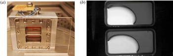
The heart of the experimental set-up consists of two identical fluid cells with interior dimensions
 $L\times 2H\times D=15~\text{mm}\times 7.5~\text{mm}\times 5~\text{mm}$
(see figure 1
a) subjected to linear vibrations. Two sidewalls of the cell are made of transparent quartz glass (Hellma), while the other four walls are custom-made from aluminium alloy. Filling or draining the cell is done through 0.5 mm holes. Safety requirements include double containment of the cells, and part of this can be seen in figure 1(a).
(a) General view of the experiment cell assembly, consisting of two identical cells filled with immiscible fluids of different viscosity and density ratios. The lower liquid layers in both cells are FC-40, while the upper layers are 2 cSt silicone oil (top cell) and 20 cSt silicone oil (bottom cell). (b) Behaviour of the interface in microgravity in the absence of vibrational forcing. Raw (cropped) image of fluid cells: heavier FC-40 (lighter region); lighter silicone oils (darker region).

Interfacial dynamics are captured by means of a charge-coupled device (CCD) camera. The lighter liquid is coloured, so images show two different grey scales corresponding to each fluid, as in figure 1(b). The camera acquisition rate is fixed at 80 frames per second, providing excellent sampling of the interface motion for low to intermediate frequencies. Below approximately 20 Hz, it is fairly easy to track the evolution of interfacial waves at a given phase, while less accurate phase resolution is achieved at the higher vibration frequencies. Nonetheless, since the oscillations of the interfacial waves are either harmonic or subharmonic, stroboscopic effects do not cause any real difficulties in identifying the mode of the instability for the frequencies considered. At the highest forcing frequency where oscillatory interfacial waves were recorded, 40 Hz, there are enough points (two and four, respectively) to distinguish harmonic from subharmonic waves, even if the phase is not known precisely.
The experiment cells and the camera are attached to a linear motor, which drives controlled translational oscillations along the
 $x$
-axis (see figure 3) of the cell at a given frequency and amplitude. The linear motor is mechanically based on a single-axis bearing positioning stage, which by specification has a maximum off-axis displacement of
 $25~\unicode[STIX]{x03BC}\text{m}$
per 300 mm. This provides an angular uncertainty in the direction of the vibrations of the order of
 $0.01^{\circ }$
. To isolate the effect of vibrations on the environment, a special 12.5 mm thick anti-vibration cork/elastomer pad is mounted between the linear motor and the rack structure. The oscillatory motion is monitored from position–time records obtained with an encoder, which permits a comparison between the nominal and real vibrational parameters.
The experimental fluid properties are detailed in table 1. Each cell holds an equal volume of FC-40 and silicone oil (either 2 cSt or 20 cSt; the upper and lower cells in figure 1, respectively). A comparison of these two fluid combinations reveals something about how viscosity and interfacial tension influence vibrational phenomena.
Physical properties of FC-40 (Flourinert Liquids™), 2 cSt silicone oil, 20 cSt silicone oil (from Someya & Munakata Reference Someya and Munakata2005), and the pairings used here. Provided are: density
 $\unicode[STIX]{x1D70C}$
, kinematic viscosity
 $\unicode[STIX]{x1D708}$
and surface tension
 $\unicode[STIX]{x1D70E}$
at
 $25\,^{\circ }\text{C}$
; thickness of the vibrational viscous boundary layers
 $\unicode[STIX]{x1D6FF}_{\unicode[STIX]{x1D708}}=\sqrt{\unicode[STIX]{x1D708}/\unicode[STIX]{x1D714}}$
for the range of parameters used; contact angle with the aluminium alloy endwalls
 $\unicode[STIX]{x1D6FD}_{A}$
(used for numerical simulations) and with the quartz glass
 $\unicode[STIX]{x1D6FD}_{G}$
. Both contact angles are estimated from image processing.

The (average) contact angle with the aluminium endwalls
 $\unicode[STIX]{x1D6FD}_{A}$
is estimated from the image processing of experimental results. The interface between FC-40 and silicone oils exhibits a finite contact angle
 $\unicode[STIX]{x1D6FD}_{G}$
with the quartz glass of the container, which can be estimated by assuming a circular arc for the cross-section:
 $$\begin{eqnarray}\displaystyle \frac{\unicode[STIX]{x03C0}}{2}-\unicode[STIX]{x1D6FD}_{G}=\tan ^{-1}\left[\frac{D\unicode[STIX]{x1D701}}{\sqrt{4\unicode[STIX]{x1D701}^{4}+\left(D/2\right)^{4}}}\right]\approx 0.074\unicode[STIX]{x03C0}. & & \displaystyle\end{eqnarray}$$
Here
 $\unicode[STIX]{x1D701}$
is the apparent interface thickness, found to be approximately equal in both cells, and
 $D$
is the cell depth. The corresponding meniscus means that the interface profile in the recorded images is not as sharp as with miscible liquids in a similar experimental set-up (Gaponenko et al.
Reference Gaponenko, Torregrosa, Yasnou, Mialdun and Shevtsova2015b
). Applied vibrations in weightlessness generally induce capillary phenomena on the length scale
 $l\sim \sqrt{\unicode[STIX]{x1D70E}/(\unicode[STIX]{x1D70C}A\unicode[STIX]{x1D714}^{2})}$
(Douady Reference Douady1990), where
 $A$
and
 $\unicode[STIX]{x1D714}$
are the driving amplitude and frequency, respectively. Variations in effective gravity and possible contact line motion drive harmonic meniscus waves. In the case of two superimposed liquids, the interfacial tension may be roughly estimated as the difference between the two corresponding liquid–air surface tensions. In table 1 the interfacial tension is relatively small and the associated meniscus effects were not noticeable in any of the experiments or simulations; for the parameter range used here
 $l\lesssim 1~\text{mm}$
. We have assumed (for simplicity) steady contact angles in the mathematical formulation of § 3.
The experiments were carried out onboard an aircraft executing parabolic manoeuvres to provide repeated periods of approximately 20 s of reduced gravity, as illustrated in figure 2. These microgravity periods are preceded by a pull-up phase and followed by a pull-out phase, each associated with approximately 20 s of hypergravity (up to 1.8
 $g_{0}$
, where
 $g_{0}=9.81~\text{m}~\text{s}^{-2}$
), and separated by several minutes of normal gravity
 $g\sim 1g_{0}$
. The microgravity level during the parabolas satisfied
 $|g_{x,z}|\leqslant 0.01g_{0}$
,
 $|g_{y}|\leqslant 0.05g_{0}$
, with the direction of the axis relative to the experiment container shown in figure 3.
Gravity profiles from one of the parabolic flights showing
 $g_{x}(t)/g_{0}$
,
 $g_{y}(t)/g_{0}$
and
 $g_{z}(t)/g_{0}$
(red, black and grey curves, respectively); see figure 3 for axes. (a) Gravity profiles together with the experiment intervals, when forcing begins both in hypergravity (yellow) and in microgravity (blue); the overlap region is shown in light green. (b) Close-up of the microgravity interval.

Each experiment, of 15 s duration, was conducted in (nearly) isothermal conditions. The temperature of the cell was measured by a negative temperature coefficient (NTC) thermistor directly fixed to the cell plate. Over the entire experimental campaign, which lasted approximately three hours, the temperature rose slightly from
 $22\,^{\circ }\text{C}$
to
 $24\,^{\circ }\text{C}$
, still very far from the mixing point of this class of liquids (Ancherbak et al.
Reference Ancherbak, Yasnou, Mialdun and Shevtsova2018). Surface tension variation over this range is less than 4 % (Someya & Munakata Reference Someya and Munakata2005), which justifies the assumption of constant surface tension over the experimental campaign.
Particular experiments were defined by a combination of fluid properties and applied forcing: frequency, amplitude and profile. The profile refers to when the forcing was initiated, i.e. whether it began during the hypergravity or microgravity portion of a particular parabolic flight. The experiment runs explored frequency and amplitude intervals of 5–50 Hz and 1–5.3 mm. Typically, experiments were repeated in different parabolas, which provided an idea of the statistical spread of the results, albeit limited by the lack of repeatability between parabolic manoeuvres.
Experiment results, although interesting and varied, were constrained by the nature of the parabolic flight: a limited number of data points (available parabolas) to explore parameter space, and the perturbed (imperfect) microgravity level. In order to investigate more frequencies and amplitudes, and to gain insight, for instance, into the importance of flight perturbations and initial conditions for the experiment outcome, a numerical model that describes immiscible fluid behaviour in the presence of vibrations is developed. The formulation and implementation are detailed in § 3 and § 4, while numerical results are discussed throughout the paper.
Sketch illustrating the (two-dimensional) numerical model.

3 Mathematical formulation
We consider two superposed horizontal layers of immiscible liquids, FC-40 and silicone oil, of equal volume and confined in a rectangular container with dimensions
 $L\times 2H=15~\text{mm}\times 7.5~\text{mm}$
, as sketched in figure 3. The cell is subjected to vibrations of amplitude
 $A$
and frequency
 $\unicode[STIX]{x1D714}$
oriented in the
 $x$
-direction. The heavier fluid, FC-40, is at the bottom so the system is gravitationally stable (in normal gravity). The physical properties of each cell are given in table 1, where the interfacial tension values have been taken from Someya & Munakata (Reference Someya and Munakata2005).
A level-set approach (Olsson & Kreiss Reference Olsson and Kreiss2005), which tracks the interface by defining a (level-set) function
 $\unicode[STIX]{x1D719}$
, is implemented to simulate the dynamics of the immiscible interface. Equation (3.1) governs its evolution, assuring conservation of interface thickness,
 $$\begin{eqnarray}\displaystyle \unicode[STIX]{x1D719}_{t}+\unicode[STIX]{x1D735}\boldsymbol{\cdot }(\boldsymbol{u}\unicode[STIX]{x1D719})=\unicode[STIX]{x1D6FE}\unicode[STIX]{x1D735}\boldsymbol{\cdot }\left(\unicode[STIX]{x1D700}\unicode[STIX]{x1D735}\unicode[STIX]{x1D719}-\unicode[STIX]{x1D719}(1-\unicode[STIX]{x1D719})\frac{\unicode[STIX]{x1D735}\unicode[STIX]{x1D719}}{|\unicode[STIX]{x1D735}\unicode[STIX]{x1D719}|}\right), & & \displaystyle\end{eqnarray}$$
where
 $\unicode[STIX]{x1D6FE}$
(units of velocity) is a tuning parameter that scales with the velocity of the interface, and
 $\unicode[STIX]{x1D700}$
is a small diffusive term added for numerical stability. The proper selection of these parameters is crucial for numerical convergence and accuracy. We set
 $\unicode[STIX]{x1D6FE}=A\unicode[STIX]{x1D714}$
for solving the vibrated problem, while
 $\unicode[STIX]{x1D700}$
is taken to be of the order of the maximum element mesh size upon convergence.
Fluid properties can be written as functions of the level-set variable
 $\unicode[STIX]{x1D719}$
via the introduction of a Heaviside function
 ${\mathcal{H}}$
(smoothed, for numerical stability),
 $$\begin{eqnarray}\displaystyle {\mathcal{H}}(\unicode[STIX]{x1D719})=\left\{\begin{array}{@{}ll@{}}\displaystyle 0,~1, & \unicode[STIX]{x1D719}<-\unicode[STIX]{x1D700},~\unicode[STIX]{x1D719}>\unicode[STIX]{x1D700},\\ \displaystyle \frac{1}{2}+\frac{\unicode[STIX]{x1D719}}{2\unicode[STIX]{x1D700}}+\frac{1}{2\unicode[STIX]{x03C0}}\sin \left(\frac{\unicode[STIX]{x03C0}\unicode[STIX]{x1D719}}{\unicode[STIX]{x1D700}}\right), & |\unicode[STIX]{x1D719}|\leqslant \unicode[STIX]{x1D700},\end{array}\right. & & \displaystyle\end{eqnarray}$$
where
 $\unicode[STIX]{x1D700}$
refers to half the interface thickness.
Density and viscosity may thus be written as
 $$\begin{eqnarray}\displaystyle & \displaystyle \unicode[STIX]{x1D70C}=\unicode[STIX]{x1D70C}_{1}+(\unicode[STIX]{x1D70C}_{2}-\unicode[STIX]{x1D70C}_{1}){\mathcal{H}}, & \displaystyle\end{eqnarray}$$
 $$\begin{eqnarray}\displaystyle & \displaystyle \unicode[STIX]{x1D707}=\unicode[STIX]{x1D707}_{1}+(\unicode[STIX]{x1D707}_{2}-\unicode[STIX]{x1D707}_{1}){\mathcal{H}}, & \displaystyle\end{eqnarray}$$
 $\unicode[STIX]{x1D719}=0,1$
, respectively.
Equations (3.1) and (3.3) are solved jointly with the continuous incompressible Navier–Stokes equations (Kothe, Mjolsness & Torrey Reference Kothe, Mjolsness and Torrey1991)
 $$\begin{eqnarray}\displaystyle & \displaystyle \unicode[STIX]{x1D70C}[\boldsymbol{u}_{t}+(\boldsymbol{u}\boldsymbol{\cdot }\unicode[STIX]{x1D735})\boldsymbol{u}]=-\unicode[STIX]{x1D735}p+\unicode[STIX]{x1D707}\unicode[STIX]{x0394}\boldsymbol{u}+\unicode[STIX]{x1D6FF}\boldsymbol{f}_{\unicode[STIX]{x1D70E}}+\unicode[STIX]{x1D70C}\boldsymbol{G}(t), & \displaystyle\end{eqnarray}$$
 $$\begin{eqnarray}\displaystyle & \displaystyle \unicode[STIX]{x1D735}\boldsymbol{\cdot }\boldsymbol{u}=0, & \displaystyle\end{eqnarray}$$
 $\unicode[STIX]{x1D70E}$
is included via
 $\boldsymbol{f}_{\unicode[STIX]{x1D70E}}$
in the momentum equation, and is given by
 $$\begin{eqnarray}\displaystyle \boldsymbol{f}_{\unicode[STIX]{x1D70E}}=(\unicode[STIX]{x1D70E}\unicode[STIX]{x1D705})\boldsymbol{n},\quad \unicode[STIX]{x1D705}=\unicode[STIX]{x1D735}\boldsymbol{\cdot }\boldsymbol{n},\quad \boldsymbol{n}=\frac{\unicode[STIX]{x1D735}\unicode[STIX]{x1D719}}{|\unicode[STIX]{x1D735}\unicode[STIX]{x1D719}|}. & & \displaystyle\end{eqnarray}$$
Here,
 $\unicode[STIX]{x1D705}$
is the interface curvature and
 $\boldsymbol{n}$
the normal vector. Interfacial effects are localised by the introduction of
 $\unicode[STIX]{x1D6FF}$
, which may be approximated in terms of the level-set function as
 $$\begin{eqnarray}\displaystyle \unicode[STIX]{x1D6FF}=|\unicode[STIX]{x1D735}\unicode[STIX]{x1D719}|. & & \displaystyle\end{eqnarray}$$
Acceleration is expressed as
 $$\begin{eqnarray}\displaystyle \boldsymbol{G}(t)=\boldsymbol{g}(t)+A\unicode[STIX]{x1D714}^{2}\cos (\unicode[STIX]{x1D714}t)\,\boldsymbol{i}, & & \displaystyle\end{eqnarray}$$
where
 $\boldsymbol{g}(t)$
refers to the (generally) time-dependent gravity field and
 $\boldsymbol{i}$
is a unit vector along the forcing axis.
Navier-slip boundary conditions, which introduce an artificial frictional force
 $\boldsymbol{f}_{\unicode[STIX]{x1D708}}=(\unicode[STIX]{x1D707}/\unicode[STIX]{x1D6FF}_{\unicode[STIX]{x1D708}})\boldsymbol{u}$
to preserve the contact angle, are applied on the walls
 $$\begin{eqnarray}\displaystyle \boldsymbol{u}\boldsymbol{\cdot }\boldsymbol{n}_{w}=0,\quad \boldsymbol{u}\boldsymbol{\cdot }[\unicode[STIX]{x1D70E}(\boldsymbol{n}_{w}-\boldsymbol{n}\cos \unicode[STIX]{x1D6FD}_{A})\unicode[STIX]{x1D6FF}]=0, & & \displaystyle\end{eqnarray}$$
where
 $\boldsymbol{n}_{w}$
is the corresponding unit normal vector,
 $\unicode[STIX]{x1D6FD}_{A}$
is the contact angle and
 $\unicode[STIX]{x1D6FF}_{\unicode[STIX]{x1D708}}=\sqrt{\unicode[STIX]{x1D708}/\unicode[STIX]{x1D714}}$
is the vibrational viscous boundary layer thickness. Crucially, these boundary conditions permit motion of the contact line, which is needed to match the experiments.
If the following scalings are used for time, length, density and viscosity,
 $$\begin{eqnarray}\displaystyle (\hat{t},\hat{\boldsymbol{x}},\hat{\unicode[STIX]{x1D70C}},\hat{\unicode[STIX]{x1D707}})=(\unicode[STIX]{x1D714}t,\boldsymbol{x}/L,\unicode[STIX]{x1D70C}/\unicode[STIX]{x1D70C}_{1},\unicode[STIX]{x1D707}/\unicode[STIX]{x1D707}_{1}), & & \displaystyle\end{eqnarray}$$
where a hat denotes dimensionless quantities, then the system dynamics (3.1)–(3.8) depend on the dimensionless frequency and amplitude
 $$\begin{eqnarray}\displaystyle \hat{\unicode[STIX]{x1D6FA}}=\frac{L^{2}\unicode[STIX]{x1D714}}{\unicode[STIX]{x1D708}_{1}},\quad \hat{A}=\frac{A}{L}, & & \displaystyle\end{eqnarray}$$
and on the other non-dimensional parameters,
 $$\begin{eqnarray}\displaystyle \widehat{\unicode[STIX]{x1D70C}}=\frac{\unicode[STIX]{x1D70C}_{2}}{\unicode[STIX]{x1D70C}_{1}},\quad \widehat{\unicode[STIX]{x1D707}}=\frac{\unicode[STIX]{x1D707}_{2}}{\unicode[STIX]{x1D707}_{1}},\quad \widehat{\unicode[STIX]{x1D70E}}=\frac{\unicode[STIX]{x1D70E}}{\unicode[STIX]{x1D70C}_{1}\unicode[STIX]{x1D714}^{2}L^{3}},\quad {\mathcal{G}}=\frac{A\unicode[STIX]{x1D714}^{2}}{g_{0}},\quad \unicode[STIX]{x1D6E4}=\frac{H}{L}, & & \displaystyle\end{eqnarray}$$
where
 $H$
is the initial height of each fluid layer (see figure 3). For the experiments of § 2, the non-dimensional parameters are shown in table 2, while frequency and amplitude are in the range of
 $$\begin{eqnarray}\displaystyle \hat{\unicode[STIX]{x1D6FA}}=[3855,32\,130]\gg 1,\quad \hat{A}=[0.0740,0.222]<1. & & \displaystyle\end{eqnarray}$$
Non-dimensional parameters corresponding to the experiments of § 2.

Finally, different initial conditions may be considered for the vibrated problem, depending on the gravity profile
 $\boldsymbol{g}(t)$
and the initialisation time of the forcing. In order to perform a consistent study based on experiments, we use the gravity profiles defined in § 4 for numerical simulations.
The commercial software COMSOL Multiphysics 5.3 is used for solving the governing equations (3.1)–(3.8) in two dimensions, written using dimensional variables, with the finite element method. Some details of the numerical method, including criteria used to select the interface thickness and meshing, are discussed in § 3.1.
The assumption of essentially two-dimensional phenomena is supported by previous modelling of the analogous vibrational problem for a similar geometry in the case of miscible fluids (Gaponenko et al.
Reference Gaponenko, Torregrosa, Yasnou, Mialdun and Shevtsova2015b
). We expect the reduced numerical model to capture the essential features of the fluid behaviour relating to both frozen waves and Faraday waves, which are the dominant phenomena observed over the relevant parameter range. The lower computational cost permits a more thorough parameter study, which is a big advantage here, although some phenomena cannot be captured. Three-dimensional irregular behaviour (with many drops) is sometimes observed experimentally with strong vibration and this is not modelled. Drop ejection, in general, is not accurately captured. In the applicable parameter regime, droplets are generated from the breaking of a fluid jet (see § 5.2 for details) and the characteristic length
 $l_{B}$
of the breaking region vanishes as the drop is ejected. The level-set formulation used here, which has a characteristic interface thickness
 $\unicode[STIX]{x1D700}$
, cannot describe the dynamics for
 $l_{B}\ll \unicode[STIX]{x1D700}$
. Drop ejection, however, is observed mainly with the FC-40 and 2 cSt silicone oil interface and represents a relatively small portion of the phenomena described below.
3.1 Convergence of the numerical solutions
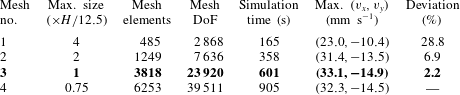
The convergence of the numerical solutions was examined for different meshes. The defining characteristics, associated numerical error and solution results are included in table 3 and illustrated in figure 4. Simulations were begun from a hydrostatic solution, with vibrations initiated during the microgravity portion of the parabola and maintained for 1.25 s. In this regime, a two-scale wave pattern develops due to a secondary Faraday instability, which occurs after the formation of a (primary) frozen wave structure.
Mesh convergence test for numerical simulations. Results for meshes nos. 1–4 are shown in blue, red, green and black, respectively. (a) Volume average of the level-set function
 $\langle \unicode[STIX]{x1D719}\rangle _{V}$
during the vibrated part of the simulation. (b) Horizontal velocity
 $v_{x}(y)$
at
 $x=4~\text{mm}$
. (c) Vertical velocity
 $v_{y}(x)$
at
 $y=3.75~\text{mm}$
.

Results of a mesh convergence test for numerical simulations of the FC-40 and 20 cSt silicone oil cell with
 $A=2~\text{mm}$
and
 $f=20~\text{Hz}$
(see § 6.1 for the relevance of this experiment). The selected mesh no. 3 is in bold, with deviations measured with respect to the maximum velocity for mesh no. 4 over the selected profiles:
 $v_{x}(y)$
at
 $x=4~\text{mm}$
and
 $v_{y}(x)$
at
 $y=3.75~\text{mm}$
. The interface thickness is
 $\unicode[STIX]{x1D700}=1.5(H/12.5)$
.

The interface thickness, which controls the scale of density and viscosity gradients across the interface (
 $\unicode[STIX]{x1D719}=0.5$
), was first varied with a fixed mesh size. The results were examined after the development of the two-scale wave pattern, and an interface thickness of
 $\unicode[STIX]{x1D700}=1.5(H/12.5)$
was selected.
The mesh was then modified by varying the maximum element size, defined as a fraction of
 $H/12.5$
, and different features were recorded in table 3: the number of mesh elements, the degrees of freedom (DoF), the simulation cost (in time) and the solution accuracy. We selected the maximum velocity of the profiles
 $v_{x}(y)$
at
 $x=4~\text{mm}$
and
 $v_{y}(x)$
at
 $y=3.75~\text{mm}$
as representative solution values, shown in figure 4(b,c), and measured the deviation from the most accurate solution. Mass conservation is checked in figure 4(a) by showing the level-set function
 $\unicode[STIX]{x1D719}$
, averaged over the fluid volume. We found mesh no. 3 to be a good compromise between computational cost and numerical accuracy. The level of numerical error with this choice should be well below that of the primary experimental uncertainties discussed in § 2.
The simulations presented throughout this paper are thus performed using a maximum element size of
 $H/12.5$
and
 $\unicode[STIX]{x1D700}=1.5(H/12.5)$
, which allows acceptable accuracy over a wide range of frequencies and amplitudes without excessive computational cost – an extended parameter study would otherwise be unfeasible. A generalised-
 $\unicode[STIX]{x1D6FC}$
(Erlicher, Bonaventura & Bursi Reference Erlicher, Bonaventura and Bursi2002) integration scheme is used, with a maximum time step manually set at
 $1/(10f)$
; this step size may be reduced (automatically), as required for stability. Both streamline (Harari & Hughes Reference Harari and Hughes1992) and crosswind (Codina Reference Codina1993) stabilisation techniques are applied.
4 Gravity profile, forcing start time and initial condition for the vibrated problem
The lack of repeatability of microgravity levels in parabolic flights (Pletser et al. Reference Pletser, Rouquette, Friedrich, Clervoy, Gharib, Gai and Mora2016) makes comparing experiments and simulations more difficult. It is hard to reproduce a specific experiment with very much precision, and such an effort would lack generality. Two of the purposes of the numerical model are to allow the exploration of a wider range of amplitudes and frequencies, where no experimental results are available, and to confirm experimental trends by means of a more systematic analysis.
Based on in situ accelerometer measurements, like those illustrated in figure 2, we define three idealised gravity profiles to be used in simulations. This permits, in some cases, a direct comparison of flight disturbances between simulations and experiments, and allows us to extend results of the model in a straightforward manner to parameters not covered by experimental data points. The three different gravity profiles used for simulations are illustrated in figure 5 by dashed curves. These profiles are mainly distinguished according to the initial and final gravity levels: ideal parabola (profile I, figure 5
a,d) when gravity only has a vertical component
 $g_{y}$
, quality parabola (profile II, figure 5
b,e) when the small lateral gravity
 $g_{x}$
decreases from
 $0.05g_{0}$
to
 $0.001g_{0}$
before the microgravity period, and generic parabola (profile III, figure 5
c,f) when lateral gravity
 $g_{x}$
decreases from
 $0.1g_{0}$
to
 $0.01g_{0}$
before the microgravity period. We use profiles I and III extensively for the simulations presented below, while profile II is used to have a more accurate model of a particular experimental result (shown later in figure 15).
Idealised two-dimensional gravity profiles
 $|g_{x}(t)|/g_{0}$
and
 $|g_{y}(t)|/g_{0}$
(dotted and dashed curves, respectively) during the initial period of a parabolic manoeuvre. Vibrational forcing (shown as solid curves, normalised to unity) may be started during microgravity (a–c) or hypergravity (d–f): (a,d) profile I, ideal parabola with
 $g_{x}=0$
; (b,e) profile II, quality parabola with final
 $g_{x}=0.001g_{0}$
; and (c,f) profile III, generic parabola with final
 $g_{x}=0.01g_{0}$
. In all profiles
 $g_{y}$
goes from
 $1.5g_{0}$
to
 $0.05g_{0}$
. Shaded regions in (a,d) show the transition (blue, duration 1.5 s) from hypergravity to microgravity and the forcing initialisation (green, duration 0.25 s), both smoothed in the manner of (3.2).

Forcing (i.e. experiments) may be initiated during microgravity or during hypergravity, as illustrated in figures 2 (blue and yellow regions) and 5 (panels a–c and d–f, respectively). The transient time required to achieve a given vibrational amplitude is 0.25 s for the computations presented in this paper. Its role in selecting the experiment outcome, possibly important in weightlessness, has not been analysed here and will be investigated elsewhere.
4.1 Quasi-equilibria driven by residual gravity
When forcing is initiated after the start of the microgravity phase of the parabolic flight, the fluids prior response to residual accelerations in the aeroplane is also captured. This allows some results concerning the (isolated) effect of flight disturbances on the shape and location of the immiscible interfaces. These states are referred to as quasi-equilibria, since the characteristic time scale of their evolution (of the order of the residual gravity variation) is significantly slower than the time scale of vibrational phenomena, especially for the medium to high frequencies used. In figures 1(b) and 6(c), some quasi-equilibria captured during the first part of a generic parabola (i.e. during the initial seconds of microgravity) are shown. The results of simulations are qualitatively consistent with the observed evolution of the interface in experiments due to varying residual gravity – illustrated in figure 6(a–c).
Interface between FC-40 and 20 cSt silicone oil (the lower experiment cell) when subjected to residual gravity. (a–c) Snapshots showing the temporal evolution of the interface when subjected solely to residual gravity during an experiment. (d–f) Simulations when subjected to the gravity profiles of figure 5 prior to initialising forcing in microgravity: (d) initial (
 $t=0.5~\text{s}$
, dashed-dotted), intermediate (
 $t=1.5~\text{s}$
, dashed) and final (
 $t=2.25~\text{s}$
, solid) interface locations for profile III (see 5
c); and (e,f) final quasi-steady equilibria selected with gravity profiles I and III, respectively.

Some computed quasi-equilibria states using gravity profiles I and III are shown in figure 6(d–f). The evolution of the interface for profile III after 0.5 s, 1.5 s and 2.25 s (see figure 5
c) is shown in (d), while (e) and (f) show the final (at
 $t=2.25~\text{s}$
) unforced quasi-equilibria for profiles I and III, respectively. These computations are qualitatively consistent with experiments. During the hypergravity period, interfaces are nearly flat except near the endwalls, where meniscus effects are dominant. The average interface (figure 6
a and dashed-dotted line in panel d) is slightly tilted with respect to the vibrational axis, with an angle of the order of a few degrees, due to the combined effect of the
 $x$
and
 $y$
components of the aeroplane acceleration. At the initiation of the microgravity phase, interface curvature develops in both cells (figure 6
b and dashed line in panel d). The heavier FC-40 fluid (nearly transparent in the image) eventually forms an asymmetric drop on the left side of the container (figure 6
c and solid line in panel d), forced by the residual acceleration in the (negative)
 $x$
-direction. The lighter silicone oil (darker shading in the image) surrounds the heavier one. Thus, the interface position is selected by a combination of residual acceleration and interfacial tension, which are comparable in effect over most of the fluid domain. The final quasi-steady states are used as initial conditions for further numerical simulations with applied vibrations. Subsequent results should thus reflect the real experiments, which are performed in this manner.
The vibrational phenomena described in the remainder of the paper are associated with noticeable differences with respect to these unforced (quasi-steady) states. Although the full picture is complex with many potential interactions, we find it useful to separate the various interfacial phenomena into those tied to fast modes, like surface waves, which oscillate on the time scale of the forcing frequency, and slow modes, like vibroequilibria and frozen waves, which are related to mean, time-averaged effects.
5 Fast-time-scale phenomena: from surface waves to drop ejection
This section considers interfacial phenomena that are associated with the forcing frequency, including both harmonic and subharmonic surface waves and the drop ejection instability that can occur with sufficient amplitude of these waves.
5.1 Interfacial waves: harmonic waves and subharmonic Faraday mode
Both harmonic and subharmonic surface waves are excited by vibrations under weightless conditions. Depending on the vibrational velocity, these waves may appear superposed on top of a frozen wave pattern, as observed in miscible fluids by Shevtsova et al. (Reference Shevtsova, Gaponenko, Yasnou, Mialdun and Nepomnyashchy2016), or a drop-like configuration evolving on a slower time scale. In figure 7, a few different interfacial modes are shown; in each frame two different out-of-phase snapshots are superimposed and the interfaces in each snapshot are outlined for clarity.
Harmonic waves are not investigated in detail here, since, except at low vibrational amplitude, they are masked by more energetic phenomena like subharmonic waves. Many of the conclusions are thus based on this higher-amplitude regime. The dynamical modes observed here typically show some degree of symmetry (see e.g. figure 7) with respect to midplane reflection, although asymmetry due to finite-size effects and residual vertical acceleration, for example, is often clearly present as well, leading to a rotation of the (average) interface position. In addition, numerical and experimental results suggest that, in many cases, surface waves form on nearly vertical portions of the interface and are of nearly constant amplitude, so that the forcing mechanism can be considered roughly homogeneous and experiments with subharmonic waves, for instance, can be compared with the ideal case of a vertically vibrated container (Kumar & Tuckerman Reference Kumar and Tuckerman1994).
Superimposed out-of-phase images for different surface wave modes with FC-40 and 2 cSt silicone oil: (a) harmonic mode at
 $f=40~\text{Hz}$
and
 $A=1.06~\text{mm}$
; (b) subharmonic mode at
 $f=5~\text{Hz}$
and
 $A=4.1~\text{mm}$
(approximately odd with respect to midplane reflection); and (c) subharmonic mode at
 $f=18~\text{Hz}$
and
 $A=1.43~\text{mm}$
(approximately even). The time between frames is labelled under each picture, while solid and dashed lines outline the interfaces in each image.

Subharmonic Faraday waves exist over a wide range of parameters and can be seen experimentally in figure 7(b,c) and, below, in figures 8 and 15(d,e). Just past onset, both experiments and simulations show supercritical small-amplitude waves whose threshold may be compared with the case of a vertically vibrated container (Faraday Reference Faraday1831; Miles & Henderson Reference Miles and Henderson1990; Kumar & Tuckerman Reference Kumar and Tuckerman1994).
In Shevtsova et al. (Reference Shevtsova, Gaponenko, Yasnou, Mialdun and Nepomnyashchy2016), the Faraday wave instability in a miscible binary mixture was analysed. The threshold of subharmonic waves was estimated based on the damped Mathieu equation (Kumar & Tuckerman Reference Kumar and Tuckerman1994) by minimising
 $$\begin{eqnarray}\displaystyle A\unicode[STIX]{x1D714}=\frac{2}{\unicode[STIX]{x1D714}k}\left(\frac{\unicode[STIX]{x1D70C}_{1}+\unicode[STIX]{x1D70C}_{2}}{\unicode[STIX]{x1D70C}_{1}-\unicode[STIX]{x1D70C}_{2}}\right)\sqrt{\left(\frac{\unicode[STIX]{x1D714}^{2}}{4}-\frac{\unicode[STIX]{x1D70E}}{\unicode[STIX]{x1D70C}_{1}+\unicode[STIX]{x1D70C}_{2}}k^{3}\right)^{2}+4k^{4}\unicode[STIX]{x1D714}^{2}\left(\frac{\unicode[STIX]{x1D707}_{1}+\unicode[STIX]{x1D707}_{2}}{\unicode[STIX]{x1D70C}_{1}+\unicode[STIX]{x1D70C}_{2}}\right)^{2}}, & & \displaystyle\end{eqnarray}$$
with
 $\unicode[STIX]{x1D70E}=0$
for the miscible fluid case.
The threshold obtained by minimising (5.1) over wavenumber provides a reference value that is later shown in figure 18 (dashed blue line) of § 7 for the experiments of § 2. There is qualitative, albeit limited, agreement of this theoretical prediction with experiment, which both display
 $f^{-1/2}$
scaling at high frequencies, although separated by a clear gap. This discrepancy is not surprising in light of the differences between theoretical assumptions and the experimental set-up, including the inhomogeneous base state (the columnar frozen wave structure) and finite-size effects. The latter become increasingly important at low frequencies, which delays onset and modifies the scaling to
 $f^{-1}$
.
The numerical simulations (dark blue solid line and blue open markers in figure 18 of § 7), on the other hand, match somewhat better with the experimental results. Numerical thresholds have been located using a similar approach as in Gandikota et al. (Reference Gandikota, Chatain, Amiroudine, Lyubimova and Beysens2014b
), using more precision in frequency and amplitude near threshold, so that the estimated uncertainty is of the order of
 $\pm 1.25~\text{Hz}$
and
 $\pm 0.0125~\text{mm}$
. For low-frequency vibrations, residual gravity can couple with the forcing to slightly modify the instability onset. This effect is observed in both cells.
Figure 8 shows a series of experimental snapshots separated by approximately one half-period of the
 $f=22~\text{Hz}$
driving force. Depending on the phase, standing waves can be seen (mainly) on the left or right side of the underlying columnar structure. The explanation for this phase shift is the sign change in the effective vibrational acceleration at each interface due to the sign of the density jump. Since the Faraday waves are subharmonic, the
 $\unicode[STIX]{x03C0}$
shift in forcing on opposite sides of the columnar structure implies a
 $\unicode[STIX]{x03C0}/2$
phase shift for the waves. The same type of behaviour was previously observed in miscible liquids (Shevtsova et al.
Reference Shevtsova, Gaponenko, Yasnou, Mialdun and Nepomnyashchy2016).
Successive snapshots showing the evolution of subharmonic Faraday waves on opposite sides of the frozen wave columnar structure for
 $f=22~\text{Hz}$
and
 $A=1.76~\text{mm}$
. Times are selected to best show the
 $\unicode[STIX]{x03C0}/2$
phase difference between these two subharmonic wave fields (
 $1/4$
period of these 11 Hz subharmonic waves is approximately 0.0227 s).

The importance of the phase difference for weakly coupled subharmonic wave fields, like these two regions of interfacial Faraday waves, was investigated in Salgado Sánchez et al. (Reference Salgado Sánchez, Porter, Tinao and Laverón-Simavilla2016). It was found that the character of the instability not only changes from supercritical to subcritical depending on detuning (most relevant here at low frequencies where the container dimensions most constrain the wavenumber), but also can change from a steady-state pitchfork bifurcation to a Hopf bifurcation due to coupling. Hopf bifurcations have not been observed here, possibly due to the coupling being too weak, and thus the modulation frequency too small, to be noticed on the time scale of the experiments and simulations.
Instability diagram of the subharmonic mode for FC-40 and 20 cSt silicone oil under different gravity profiles: (a) profile I and (b) profile III. Experimental (filled circles) and numerical (open circles) results exhibit various dynamical modes, marked with alternating blue tones. The solid curves are drawn for visual reference to distinguish different average vertical wavenumbers. The dashed curve indicates that all these modes belong to the main subharmonic instability tongue. Illustrative snapshots in the upper left corner show the initial condition, while the smaller images show the interface after
 $t\approx 2~\text{s}$
of applied vibration in microgravity.

By combining numerical with experimental results, we are able to construct the instability diagram for the subharmonic Faraday wave mode in each experiment cell. In figure 9, results for FC-40 and 20 cSt silicone oil are organised by the wavenumber
 $k$
measured in the centre of the pattern and vibrational velocity under gravity profiles I (panel a) and III (panel b). Four modes are distinguished according to the average number of wavelengths in the vertical direction, and corresponding curves are drawn for visual reference, suggesting boundaries within the main subharmonic tongue. Since the simulations of figure 9(a) are performed using the ideal gravity profile (no
 $g_{x}$
component), they are not compared directly with experiments, but provide a reference for evaluating the effect of residual gravity seen in figure 9(b), which shows results obtained using a more generic gravity profile that may be better compared to experiments. We note that numerical simulations near
 $k=1~\text{mm}^{-1}$
were not able to reproduce subharmonic waves as seen in experiments, perhaps due to the increased importance of residual gravity at those low forcing amplitudes in the experiments or to increased damping from the boundaries in the simulations. Over the limited region of overlap, the experimental results are consistent with the simulations, in terms of both wavenumber selection and the qualitative structure of the surface.
As discussed in Batson et al. (Reference Batson, Zoueshtiagh and Narayanan2013), gravity plays a dual role in shaping the instability diagram, modifying not only the instability threshold but also the location and profile of the mode boundaries. The effect of gravity can be seen in figure 9 by comparing the response of the interface to the two different microgravity profiles. When a small disturbance is introduced along the
 $x$
-axis (figure 9
b, profile III), the mode boundaries shift a bit towards lower wavenumbers (frequencies), while the threshold is modified only slightly. Note that the conditions differ only in the gravity level along the
 $x$
-direction, which is
 $0.01g_{0}$
for profile III. Some differences with respect to the predictions of Batson et al. (Reference Batson, Zoueshtiagh and Narayanan2013) are expected. Also note that, compared to the analysis of Batson et al. (Reference Batson, Zoueshtiagh and Narayanan2013) and Kumar & Tuckerman (Reference Kumar and Tuckerman1994), we only locate the subharmonic instability tongue, which is normally dominant in Faraday wave systems, and this is shown with the (dashed black) curve in figure 9. Other instability tongues (harmonic, for example) are masked by the primary subharmonic mode and difficult to observe.
Instability diagram for the subharmonic mode with FC-40 and 2 cSt silicone oil under gravity profile I. Experimental data (filled circles) and numerical simulations (open circles) reveal various dynamical modes, marked with alternating blue tones. The solid curves are drawn for visual reference to distinguish different average vertical wavenumbers. The dashed curve indicates that all these modes belong to the main subharmonic instability tongue. Illustrative snapshots in the upper left corner show the initial condition, while the smaller images show the interface after
 $t\approx 2~\text{s}$
of applied vibration in microgravity.

Viscous and interfacial tension effects are revealed in a comparison of figures 9(a) and 10. Lower viscosity clearly reduces the threshold for Faraday waves. At the same time, the reduction of interfacial tension with 2 cSt silicone oil generally increases the observed wavenumber of the subharmonic mode (for a given forcing frequency). This is consistent with the dispersion relation, and is investigated experimentally, for example, in Gandikota et al. (Reference Gandikota, Chatain, Amiroudine, Lyubimova and Beysens2014a ), where the wavenumber of the Faraday instability in near-critical hydrogen is observed to increase with approach to the critical point where interfacial tension vanishes.
As vibrational velocity increases, the subharmonic Faraday waves become increasingly nonlinear and, at sufficient velocity, interfacial integrity breaks down, initiating a process of drop ejection. This process is important, since it places an upper bound on the wave amplitudes that can be investigated experimentally and numerically.
5.2 Drop ejection instability of the subharmonic mode
At large enough amplitude, the increasingly nonlinear Faraday waves may become unstable to drop ejection (Goodridge, Shi & Lathrop Reference Goodridge, Shi and Lathrop1996; Goodridge et al. Reference Goodridge, Shi, Hentschel and Lathrop1997; James et al. Reference James, Vukasinovic, Smith and Glezer2003b ). Visual observations indicate that the resulting interfacial pattern often has a three-dimensional structure, which makes the two-dimensional simulations less applicable. Despite the complexity of this process, especially when many drops are present, the experimental results allow us to distinguish two qualitatively different instability mechanisms that are associated with distinct velocity thresholds:
(i) A – heavier-to-lighter liquid ejection when a drop of FC-40 is ejected into the bulk of the silicone oil.
(ii) B – lighter-to-heavier liquid ejection when a drop of silicone oil is ejected into the bulk of the FC-40 fluid.
Representative snapshots in time (values provided) showing the different drop ejection mechanisms observed in the FC-40 and 2 cSt silicone oil cell during microgravity: (a–c) mechanism A (near onset), (d–f) mechanism A (far from onset), and (g–i) mechanism B.

The dynamics of mechanism A is shown in figure 11(a–c) for
 $A=1.57~\text{mm}$
and
 $f=20~\text{Hz}$
. In this process, drops are created in the lighter fluid and ejected away from the interface. A variation of mechanism A can occur with larger vibrational velocities, as in figure 11(d–f) with
 $A=4.29~\text{mm}$
and
 $f=8~\text{Hz}$
, where drops are still created in the lighter fluid but, instead of moving away, tend to remain trapped near the interface.
Mechanism B occurs for larger amplitudes, sometimes concurrently with mechanism A. The dynamics of the process are as shown in figure 11(g–i) for
 $A=4.37~\text{mm}$
and
 $f=9~\text{Hz}$
.
Drop ejection is associated with a jet of fluid emerging from a large-amplitude surface wave that then collapses to create a drop of fluid and, often, other smaller drops, which are known as satellites (James et al.
Reference James, Vukasinovic, Smith and Glezer2003b
; Castrejón-Pita et al.
Reference Castrejón-Pita, Castrejón-Pita, Thete, Sambath, Hutchings, Hinch, Lister and Basaran2015). As forcing amplitude is increased, especially if it becomes comparable to (or larger than) the thickness of the liquid layer,
 $A>H$
, the scenario can be very complex. The dynamics is often fully three-dimensional and disordered in this regime (James et al.
Reference James, Smith and Glezer2003a
) and the drops interact with the strongly nonlinear subharmonic waves and the associated mean flow, which can lead to the drop being recaptured by the interface. We note that the highly nonlinear behaviour of the system for
 $A>H$
was also observed in the case of miscible liquids, which led either to secondary Faraday waves over frozen waves (Shevtsova et al.
Reference Shevtsova, Gaponenko, Yasnou, Mialdun and Nepomnyashchy2016) or to the formation of a fish-spine pattern (Shevtsova et al.
Reference Shevtsova, Gaponenko, Yasnou, Mialdun and Nepomnyashchy2015b
).
Drop ejection instability thresholds for FC-40 and 2 cSt silicone oil as a function of frequency
 $f$
and (a) amplitude
 $A$
and (b) vibrational velocity
 $A\unicode[STIX]{x1D714}$
. Circles mark experimental data points, coloured in red if drop ejection is found. Fits using different scalings for the drop ejection threshold (mechanism A, dashed black line) are given in colour:
 $A\propto f^{-1}$
(red),
 $A\propto f^{-2/3}$
(green) and
 $A\propto f^{-1/2}$
(blue). The threshold curve for mechanism B (solid black line) is estimated from experiments (no scaling assumptions).

The thresholds of the two droplet ejection mechanisms identified above are shown in figure 12 for FC-40 and 2 cSt silicone oil in terms of amplitude
 $A$
(panel a) and vibrational velocity
 $A\unicode[STIX]{x1D714}$
(panel b) versus frequency
 $f$
. The estimated thresholds shown are based on the available experimental data points (filled circles). The dashed black curve indicates the lower bound of the droplet ejection regime, while the solid black curve indicates the onset of mechanism B. For the majority of low-gravity experiments considered here, performed at
 $f<15~\text{Hz}$
, wave breaking with drop ejection is observed at
 $A\unicode[STIX]{x1D714}|_{c}\gtrsim 0.17~\text{m}~\text{s}^{-1}$
, as illustrated in figure 12(b).
We can compare the experimental results giving the (estimated) onset of drop ejection with the scalings suggested by Goodridge et al. (Reference Goodridge, Shi, Hentschel and Lathrop1997) for the cases of a system dominated by surface tension (with, for example, low-viscosity fluids like ethanol), i.e.
 $A\unicode[STIX]{x1D714}\sim c_{1}F_{1}(\unicode[STIX]{x1D70E}/\unicode[STIX]{x1D70C})\unicode[STIX]{x1D714}^{1/3}$
, and for more viscous fluids (like water or glycerine), i.e.
 $A\unicode[STIX]{x1D714}\sim c_{2}F_{2}(\unicode[STIX]{x1D708})\unicode[STIX]{x1D714}^{1/2}$
. We also consider a constant velocity threshold,
 $A\unicode[STIX]{x1D714}\sim c_{3}~(=0.17~\text{m}~\text{s}^{-1})$
. Here
 $c_{j},~j=1,2,3$
, are constants while
 $F_{1}(\unicode[STIX]{x1D70E}/\unicode[STIX]{x1D70C})=(\unicode[STIX]{x1D70E}/\unicode[STIX]{x1D70C})^{1/3}$
and
 $F_{2}(\unicode[STIX]{x1D708})=\sqrt{\unicode[STIX]{x1D708}}$
for a single-fluid system. The corresponding prefactors are obtained by fitting, and the results are shown in figure 12(b).
The results, although limited by the small number of experimental data points and the variable conditions onboard the parabolic flight (e.g. residual gravity effects), do suggest a transition from (nearly) constant critical velocity at low frequencies to an increase of critical velocity (most) consistent with the scaling proposed by Goodridge et al. (Reference Goodridge, Shi, Hentschel and Lathrop1997) for viscous fluids. Note that more experimental data points would be needed to more clearly determine the scaling definitively and that, in any case, there are substantial differences between the experiments of § 2 and the system considered by Goodridge et al. (Reference Goodridge, Shi, Hentschel and Lathrop1997), which would affect the
 $c_{i}$
and
 $F_{i}$
factors.
In the limit of high frequency, equation (5.1) gives a reference value for subharmonic Faraday waves, while experiments suggest a roughly constant gap between the onset of Faraday waves and the drop ejection instability (both scale approximately as
 $f^{-1/2}$
for higher frequencies). The regularity of this gap can be seen later in figure 18 of § 7 with the solid blue and red lines. Ignoring the details associated with both instabilities (see e.g. Goodridge et al.
Reference Goodridge, Shi, Hentschel and Lathrop1997), the results suggest that the energy gap between Faraday waves and drop ejection depends only weakly on the frequency of the forcing, and mainly on the physical properties of the fluid. Since the less viscous combination of FC-40 and 2 cSt silicone oil allows more data points in the drop ejection regime, conclusions are drawn mainly from this case.
5.3 Energy estimation for drops and interfacial phenomena
For the experiments described in § 2, drop ejection generally occurs after the interface has evolved towards a columnar or bubble-like structure, and then undergone an instability to Faraday waves. This means that the average interface is constrained by the system size – reaching from top to bottom and oriented, to a large extent, perpendicular to the forcing. Both contact energy, which is relevant when
 $\unicode[STIX]{x1D6FD}\neq \unicode[STIX]{x03C0}/2$
, and the average interfacial energy are largely constrained (bounded) in this situation. An increase in interfacial energy must manifest through the dynamics of the interface via higher-amplitude waves or drop ejection.
We estimate the interfacial energy of the main interface and of the drops after ejection begins (
 $A\unicode[STIX]{x1D714}>A\unicode[STIX]{x1D714}|_{c}\approx 0.17~\text{m}~\text{s}^{-1}$
for
 $f<15~\text{Hz}$
) by measuring the visible interface length in selected frames of each experiment run. Consistent with the two-dimensional approximation (near onset, at least, the subharmonic waves do appear to be quasi-two-dimensional), we assume that the contribution from the perpendicular dimension
 $D$
is constant for different interface positions and for the initial drops. With this simplifying approximation, the interfacial energy depends on its visible perimeter, which can be measured in a given snapshot simply by summing pixels:
 $E_{S}\sim \unicode[STIX]{x1D70E}{\mathcal{P}}_{\unicode[STIX]{x1D70E}}$
, where
 ${\mathcal{P}}_{\unicode[STIX]{x1D70E}}$
is the pixel count of the perimeter. In figure 13, the measured interfacial energies (sum of visible lengths) of the main average interface (green squares), neglecting surface waves, and the drops (red circles) are given as a function of
 $$\begin{eqnarray}\displaystyle \unicode[STIX]{x1D6FF}_{c}=A\unicode[STIX]{x1D714}-A\unicode[STIX]{x1D714}|_{c}, & & \displaystyle\end{eqnarray}$$
where
 $A\unicode[STIX]{x1D714}|_{c}$
is the drop ejection threshold.
Interfacial energies, measured by
 ${\mathcal{P}}_{\unicode[STIX]{x1D70E}}$
(in pixels), obtained for FC-40 and 2 cSt silicone oil, as a function of
 $\unicode[STIX]{x1D6FF}_{c}=A\unicode[STIX]{x1D714}-A\unicode[STIX]{x1D714}|_{c}$
, where
 $A\unicode[STIX]{x1D714}|_{c}$
is the drop ejection threshold found to be
 $0.1743~\text{m}~\text{s}^{-1}$
from the fit. The interfacial energies of the drops (red circles) and the main interface (green squares) are included. The curves are fitted to quadratic and constant functions, respectively. The number of observed drops is marked in parentheses, while outlier data points marked with crosses are excluded from the fit.

As expected, we find that the main interfacial energy term is (nearly) constant since either the frozen wave instability has led to columnar structures, or the vibroequilibria effect has flattened an initially bubble-like configuration. In both cases, the main interfacial energy is bounded by the system size. Drop energy, in contrast, increases (roughly) as
 $\unicode[STIX]{x1D6FF}_{c}^{2}$
, as shown by a quadratic fitting to the experimental points.
We note several uncertainties of the experiments, which were not designed to study drop ejection, and of the fit in figure 13. First, drop number and size varied even near onset, and the significant interfacial energy of a single drop means that
 ${\mathcal{P}}_{\unicode[STIX]{x1D70E}}$
does not go to zero at onset, but jumps to a finite value instead. Also, some runs were excluded as outliers (marked by crosses in figure 13). Upon checking the corresponding datasets, we attribute these exceptions to the lack of repeatability in the residual gravity profile between parabolas, and to the potential hysteresis that occurs if drops survive between parabolas. The former modifies the contribution of gravity (neglected in the analysis) and may eventually interact with the drops (James et al.
Reference James, Smith and Glezer2003a
) if a change in gravity couples with the ejection process, for example. Hysteresis is problematic too, with the experiment starting from a metastable initial condition, which changes the evolution (and energies) of the phenomena involved.
One can try to understand the results of figure 13 by recalling the energy balance suggested by the theory of vibroequilibria (Lyubimov et al. Reference Lyubimov, Cherepanov, Lyubimova and Roux1997; Beyer et al. Reference Beyer, Gawriljuk, Günther, Lukovsky and Timokha2001; Gavrilyuk et al. Reference Gavrilyuk, Lukovsky and Timokha2004), where selection of the time-average (quasi-static) interface shape is formulated as a minimisation problem using a Lagrangian method that considers vibrational and surface energy contributions, among others (like gravitational); surface waves, which do not affect the average interface (to leading order), are not accounted for.
Assuming constant interfacial tension, the system energy
 $E$
may be expressed (see e.g. Fernández et al.
Reference Fernández, Tinao, Porter and Laverón-Simavilla2017b
) in a co-moving frame as
 $$\begin{eqnarray}\displaystyle E=(\unicode[STIX]{x1D70C}_{1}-\unicode[STIX]{x1D70C}_{2})\unicode[STIX]{x1D700}(S)(A\unicode[STIX]{x1D714})^{2}+\unicode[STIX]{x1D70E}\int _{S}\unicode[STIX]{x2202}S+\cdots \,, & & \displaystyle\end{eqnarray}$$
where
 $\unicode[STIX]{x1D700}(S)$
represents a non-dimensional factor obtained by integrating over the fluid domain (determined by the walls and interface
 $S$
) and suppressed terms (signified by dots) include contact energy and gravitational energy.
In the absence of gravity and other relevant forces, the principal balance is between vibrational energy, which increases as
 $(A\unicode[STIX]{x1D714})^{2}$
, and interfacial energy. At a minimum of the Lagrangian (the vibroequilibria solution), these two energy terms have equal and opposite derivatives with respect to any (small continuous) variation. A finite increase in forcing will directly increase the vibrational energy of the system and this will, in turn, cause the interface to reorient, increasing interfacial energy but decreasing vibrational energy until a new balance (minimum) is achieved. Neglecting the initial interfacial contribution (of a flat, unforced interface, for instance), the interfacial energy of a vibroequilibria solution is expected to scale as
 $(A\unicode[STIX]{x1D714})^{2}$
.
It is interesting to note that the balance suggested by vibroequilibria theory, with increases in vibrational energy being partly transferred into (average) interfacial energy, seems to be replaced by an analogous process for drop ejection. Following a nonlinear process in which the surface wave amplitude increases until breaking occurs, subsequent increases in vibrational energy are partly channelled into the creation of ejected drops, with the
 $(A\unicode[STIX]{x1D714})^{2}$
scaling carried over as well when the shifted value
 $\unicode[STIX]{x1D6FF}_{c}=A\unicode[STIX]{x1D714}-A\unicode[STIX]{x1D714}|_{c}$
is used.
6 Slow-time-scale phenomena: the frozen wave instability and vibroequilibria
When horizontal vibrations are applied to immiscible layers of fluids with a flat interface, Lyubimov & Cherepanov (Reference Lyubimov and Cherepanov1986) predicted, in the inviscid limit, the appearance of standing (sinusoidal) waves, known as frozen waves, at a certain velocity threshold. In deep layers the critical wavelength is the capillary length. The absence of a strong (gravitational) restoring force in weightlessness means that these initially sinusoidal patterns can develop into large columnar structures. The length scale of these structures is bounded by the size of the system and reflects the wavelength of the fastest-growing perturbation for a given forcing (Lyubimova et al. Reference Lyubimova, Ivantsov, Garrabos, Lecoutre, Gandikota and Beysens2017). Here, we show experimental evidence of the frozen wave instability in microgravity and hypergravity, and present numerical results, particularly in connection with the wavenumber selected in the instability.
The vibroequilibria effect is also a potentially important slow-time-scale phenomenon in microgravity. Although we observe some evidence of vibroequilibria in the experiments of § 2, such as a flattening of the drop-like configurations, the presence of residual gravity perturbations and the strong effect of the frozen wave instability for higher vibrational velocities makes it difficult to isolate their effects or to quantify them in a precise manner. We expect that vibroequilibria effects, insofar as they tend to cause the interface to orient more perpendicular to the axis of vibration, have a stabilising effect on the frozen wave instability, whose (Kelvin–Helmholtz type) mechanism supposes an interface aligned with the axis of vibration.
6.1 Frozen waves and the two-scale wave pattern
The series of snapshots in figures 14 and 15 show the evolution of the interface between immiscible liquids subjected to horizontal vibrations under microgravity conditions. Each figure contains experimental observations for
 $f=22~\text{Hz}$
that confirm the results of simulations for
 $f=20~\text{Hz}$
. It is clear that the amplitude, which is below the threshold for frozen waves in figure 14 and above this threshold in figure 15, has a big effect. Increasing from
 $A=0.87~\text{mm}$
to
 $A=1.76~\text{mm}$
in the experiments (from
 $A=1.5~\text{mm}$
to
 $A=2.0~\text{mm}$
in simulations) pushes the system beyond the critical value for the frozen wave instability. Recall that this instability is caused by a shear-driven mechanism similar to the Kelvin–Helmholtz instability.
Snapshots showing temporal evolution of the FC-40 and 20 cSt silicone oil interface below the frozen wave threshold for both experiments and simulations. (a–c) Experiment response at
 $f=22~\text{Hz}$
and
 $A=0.87~\text{mm}$
. (d–f) Simulation performed at
 $f=20~\text{Hz}$
and
 $A=1.5~\text{mm}$
under gravity profile III. A comparison of experiment and simulations in time cannot be done quantitatively due to the definition of
 $\boldsymbol{g}(t)$
(see § 4), so time values are not labelled.

Snapshots showing temporal evolution of the FC-40 and 20 cSt silicone oil interface above the frozen wave threshold for both experiments and simulations. (a–e) Experiment response at
 $f=22~\text{Hz}$
and
 $A=1.76~\text{mm}$
(above frozen wave onset) showing the growth of the instability (a,c) and the secondary Faraday waves excited on the lateral boundaries of the columns. The snapshots (d,e) separated by
 $\unicode[STIX]{x0394}t=0.05~\text{s}\approx 1/(22~\text{Hz})$
show the (nearly) out-of-phase subharmonic behaviour; waves on the right column are shifted in phase by
 $\unicode[STIX]{x03C0}/2$
. (f–h) Simulation performed at
 $f=20~\text{Hz}$
and
 $A=2~\text{mm}$
under gravity profile II. A comparison of experiment and simulations in time cannot be done quantitatively due to the definition of
 $\boldsymbol{g}(t)$
(see § 4), so the time values are not labelled.

Below the frozen wave threshold (figure 14), residual gravity drives the formation of a squeezed drop-like structure located near the left side of the cell. Subsequently, either harmonic surface waves (figure 14 a,b,d,e) or Faraday waves (figure 14 f) may be excited over the interface; see § 5.1 for further details.
Above the frozen wave threshold (figure 15), the interface forms a pattern with
 $\unicode[STIX]{x1D706}\sim L$
, which then develops into a columnar-like structure. Subharmonic Faraday waves (see § 5.1) can appear on both sides of a column (figure 15
d,e). Analogous two-scale patterns have been observed in miscible fluid experiments (Shevtsova et al.
Reference Shevtsova, Gaponenko, Yasnou, Mialdun and Nepomnyashchy2016).
The (numerical) onsets of Faraday (dark blue circles and dark blue solid line in figure 18) and frozen waves (green squares and green solid line in figure 18) cross at a frequency
 $f^{\ast }\sim 35~\text{Hz}$
for 2 cSt silicone oil and
 $f^{\ast }\sim 17.5~\text{Hz}$
for 20 cSt silicone oil. If we imagine an idealised scenario with
 $\unicode[STIX]{x1D6FD}=\unicode[STIX]{x03C0}/2$
and an initially flat interface in microgravity, then Faraday waves cannot immediately appear with horizontal excitation (although harmonic and cross-waves can), even if their threshold is surpassed. It is only after frozen waves have been excited that columnar structures develop and portions of the interface are sufficiently perpendicular to the forcing axis to permit the excitation of Faraday waves. Thus, for
 $f<f^{\ast }$
one expects, with increasing amplitude, to first see the frozen wave instability, quickly followed (at sufficient wave amplitude) by Faraday waves – the frozen wave instability acts here, among other things, to facilitate or ‘trigger’ Faraday waves by reorienting the interface. For
 $f>f^{\ast }$
, on the other hand, the frozen waves develop free of Faraday waves, whether forming columnar structures or not, until the Faraday wave threshold is crossed. In a real parabolic flight experiment, however, plane manoeuvres and residual gravity do not permit a purely horizontal flat interface, and the situation is more complex. Faraday waves may appear any time a portion of the interface moves towards a (nearly) perpendicular orientation with respect to the vibrational axis and the Faraday wave threshold is exceeded.
Although some experiments were performed above the frozen wave threshold (see figure 18), the irregular microgravity conditions in those runs do not permit a satisfactory analysis of the instability. In addition, with the 2 cSt silicone oil, the experiments performed above the frozen wave threshold are complicated by high-amplitude Faraday waves or drop ejection, making the results hard to process. Here, we perform a simulation-based analysis of frozen waves and compare it, when possible, with experimental results and theoretical predictions. Unlike the experiments of § 2, we analyse the instability under idealised microgravity conditions (mainly, profile I) in the numerical model.
6.2 The frozen wave instability in microgravity
Columnar-like structures developing from the frozen wave instability have been seen in previous experiments in microgravity either in ordinary miscible liquids (Gaponenko et al. Reference Gaponenko, Torregrosa, Yasnou, Mialdun and Shevtsova2015b ) or in near-critical fluids where interfacial tension vanishes (Gandikota et al. Reference Gandikota, Chatain, Amiroudine, Lyubimova and Beysens2014a ,Reference Gandikota, Chatain, Amiroudine, Lyubimova and Beysens b ). Here we report, for the first time, columnar-like structures in microgravity for a pair of liquids with sizeable interfacial tension.
Previous treatments and investigations of frozen waves (Lyubimov & Cherepanov Reference Lyubimov and Cherepanov1986; Talib et al. Reference Talib, Jalikop and Juel2007; Goldobin et al. Reference Goldobin, Pimenova, Kovalevskaya, Lyubimov and Lyubimova2015; Lyubimov et al. Reference Lyubimov, Ivantsov, Lyubimova and Khilko2016) considered a sufficiently large container or the ideal case of an infinite domain so that finite-size effects could be neglected. In this limit, a linear stability analysis provides the velocity threshold
 $$\begin{eqnarray}\displaystyle (A\unicode[STIX]{x1D714})^{2}=\frac{(\unicode[STIX]{x1D70C}_{1}+\unicode[STIX]{x1D70C}_{2})^{3}}{\unicode[STIX]{x1D70C}_{1}\unicode[STIX]{x1D70C}_{2}(\unicode[STIX]{x1D70C}_{1}-\unicode[STIX]{x1D70C}_{2})}\sqrt{\frac{\unicode[STIX]{x1D70E}g_{y}}{\unicode[STIX]{x1D70C}_{1}-\unicode[STIX]{x1D70C}_{2}}}, & & \displaystyle\end{eqnarray}$$
for the inviscid case. The most unstable wavenumber
 $k=\sqrt{(\unicode[STIX]{x1D70C}_{1}-\unicode[STIX]{x1D70C}_{2})g_{y}/\unicode[STIX]{x1D70E}}$
is related to the capillary length. When vibrated beyond the threshold (6.1), which is very small in microgravity, wavenumber selection depends on the vibrational velocity, which excites a band of wavenumbers. In Burnysheva, Lyubimov & Lyubimova (Reference Burnysheva, Lyubimov and Lyubimova2011), it was assumed that the wavelength selection in this problem was defined by the perturbation with maximum growth rate. A continuous and monotonic relationship between vibrational velocity and selected wavenumber was found.
In order to compare experiments and simulations with this theoretical prediction, figure 18 includes (6.1) with
 $g_{y}=0.05g_{0}$
(green dashed lines) for each experimental cell. Theoretical predictions give
 $$\begin{eqnarray}\displaystyle A\unicode[STIX]{x1D714}|_{theory}=0.134~\text{m}~\text{s}^{-1}~(2~\text{cSt oil}),\quad 0.1581~\text{m}~\text{s}^{-1}~(20~\text{cSt oil}), & & \displaystyle\end{eqnarray}$$
while the numerical results (green solid lines) yield
 $$\begin{eqnarray}\displaystyle A\unicode[STIX]{x1D714}|_{experiment}=0.157~\text{m}~\text{s}^{-1}~(2~\text{cSt oil}),\quad 0.207~\text{m}~\text{s}^{-1}~(20~\text{cSt oil}). & & \displaystyle\end{eqnarray}$$
Our results are in line with findings by Talib et al. (Reference Talib, Jalikop and Juel2007) that inviscid predictions underestimate the true onset value, which is affected by viscosity and, due to the geometry of the experiment cells, finite-size effects. The results here are obtained in relatively small containers where finite-size effects are expected to be important. To investigate this, the wavenumber of the instability is shown in figure 16(a) alongside the vibrational velocity with gravity profile I (
 $g_{x}=0$
) and for each fluid combination.
For small amplitudes, a constant wavenumber
 $k_{1}\sim 0.4~\text{mm}^{-1}$
(
 $\unicode[STIX]{x1D706}_{1}\sim 15.7~\text{mm}\approx L$
) is observed in both cells. When compared to the inviscid theory, it is evident that the wavenumber selection is driven by the container length. This wavenumber is nearly constant with increasing velocities until a certain value
 $A\unicode[STIX]{x1D714}\sim 0.3~\text{m}~\text{s}^{-1}$
is reached, at which point the wavenumber doubles to
 $k_{2}\sim 0.8~\text{mm}^{-1}$
. For this second mode, the results exhibit a certain amount of dispersion in the less viscous combination (green squares), while the wavenumber is nearly constant for the more viscous case (red squares). This mode persists until a velocity of
 $A\sim 1~\text{m}~\text{s}^{-1}$
, where the wavenumber appears to double again.
(a) Frozen wave instability diagram showing wavenumber for both combinations (less viscous, green open squares) under gravity profile I, when vibrations are applied in microgravity. (b) Frozen wave instability diagram for FC-40 and 20 cSt silicone oil under different gravity profiles and forcing initiation times: profile I initiation in microgravity (red open squares), profile I initiation in hypergravity (pink open squares), and profile III initiation in hypergravity (cyan open squares). An experimental measurement (black solid square) is also shown. Illustrations are included to help visualise the features of the instability.

6.3 Residual gravity effects
The effect of residual gravity is analysed here and compared to the available experimental data point. In figure 16(b), the wavenumber of the frozen wave instability under different gravity conditions (i.e. gravity profiles) and forcing initiation times is shown for FC-40 and 20 cSt silicone oil.
First, note the differences arising from the initiation time of the forcing. This is shown for gravity profile I, both for initiation during the hypergravity period (pink open squares) and during microgravity (red open squares). Despite the fact that the final gravity level is identical for both experiments, the wavenumber at onset is distinct. For hypergravity initialisation, when
 $g_{y}$
is reduced after the vibration begins, the frozen wave threshold, which depends on
 $g_{y}$
via equation (6.1), may be surpassed before the final microgravity level is reached. Since the vertical gravity at this instant is larger, an increased wavenumber is expected. This wavenumber is nearly constant before jumping at a certain velocity, as in the previous case.
With increased vibrational velocity in this hypergravity case, we observe greater dispersion in the wavenumber, which may be explained in the same way. The variation of the gravity level results in varying (most dangerous) wavenumbers and so, depending on the growth rate of each unstable mode and its interaction with the changing gravity level, different final states may be found. In particular, a new mode is observed with
 $k\sim 1.2~\text{mm}^{-1}$
.
In the case of gravity profile III (cyan open squares), when there is a perturbation in the
 $x$
-direction, a further increase in
 $k$
is observed. In addition to that, the critical velocities for transition to different modes are notably increased as well; this limits the maximum expected wavenumber in experiments. We were able to process just one experimental point (black solid square), where the microgravity conditions of the parabola allowed the appropriate development of frozen waves.
To the best of our knowledge, the results presented here are the first to examine the effect of residual gravity and strong finite-size constraints on wavenumber selection for the frozen wave instability.
6.4 The frozen wave instability in hypergravity
Only one experiment run considered high-frequency and high-amplitude vibrations. Despite the scarcity of experimental data points in this regime, which was further aggravated by the fact that the run was quickly aborted for safety considerations, there is clear evidence of the frozen wave instability in both experimental cells. In figure 17, three snapshots of each cell after initiation of the forcing in hypergravity are shown; the excitation is with
 $f=50~\text{Hz}$
and
 $A=3.9~\text{mm}$
.
As with lower vibrational velocities, there may be a harmonic surface wave mode, typical of horizontally vibrated containers (see e.g. Porter et al.
Reference Porter, Tinao, Laverón-Simavilla and López2012; Salgado Sánchez et al.
Reference Salgado Sánchez, Porter, Tinao and Laverón-Simavilla2016), directly excited on the interface during hypergravity (figure 17
a,d). These surface waves, which are strongly nonlinear here, seem to propagate inwards from the ends of the container, but quickly evolve towards a different fluid configuration over a characteristic time
 $\unicode[STIX]{x1D70F}<0.0125~\text{s}$
during the hypergravity period, as illustrated in figure 17(b,e). Here, the weightlessness condition is less significant since the vibrational amplitude is so large, effectively dominating over gravity and allowing the formation of a nearly columnar pattern. The ratio of the estimated frozen wave instability wavenumber for the two experiments (2 cSt oil, figure 17
b, denoted by subscript 1; 20 cSt oil, figure 17
e, denoted by subscript 2) is measured as
 $$\begin{eqnarray}\displaystyle \left.\frac{k_{1}}{k_{2}}\right|_{experiment}=\frac{\unicode[STIX]{x1D706}_{2}}{\unicode[STIX]{x1D706}_{1}}\approx 1.26, & & \displaystyle\end{eqnarray}$$
which matches well with the predictions of Lyubimov & Cherepanov (Reference Lyubimov and Cherepanov1986):
 $$\begin{eqnarray}\displaystyle \left.\frac{k_{1}}{k_{2}}\right|_{theory}=\sqrt{\frac{\unicode[STIX]{x1D70E}_{2}(\unicode[STIX]{x1D70C}_{1}-\unicode[STIX]{x1D70C}_{2})_{1}}{\unicode[STIX]{x1D70E}_{1}(\unicode[STIX]{x1D70C}_{1}-\unicode[STIX]{x1D70C}_{2})_{2}}}\approx 1.29. & & \displaystyle\end{eqnarray}$$
With FC-40 and 2 cSt silicone oil, the frozen wave pattern coexists with numerous drops near the interface. In the case of the higher-viscosity 20 cSt silicone oil, however, the Faraday waves do not reach high enough amplitude to cause drop ejection in less than 0.0125 s (one could speculate that, had the experiment lasted longer, they would have). In figure 18(b), this experimental point is included for the sake of completeness, but marked in blue to emphasise the discrepancy with expected phenomena in this regime.
Three snapshots, separated by 0.0125 s in time for FC-40 and 2 cSt silicone oil (a–c) and FC-40 and 20 cSt silicone oil (d–f) subjected to vibrations at
 $f=50~\text{Hz}$
and
 $A=3.9~\text{mm}$
. (a,d) Initial high-amplitude surface waves in hypergravity, (b,e) transient frozen wave pattern (in hypergravity), and (c,f) transition from vibrated to residual gravity equilibria.

Response of the fluid interface to vibrations in microgravity as a function of frequency
 $f$
and amplitude
 $A$
: (a) FC-40 and 2 cSt silicone oil, and (b) FC-40 and 20 cSt silicone oil. Solid circles denote experimental points in three regimes: harmonic waves (yellow), subharmonic Faraday waves (blue) and drop ejection (red). Open markers denote numerical results for the Faraday wave instability (blue open circles) and the frozen wave instability (green open squares). These thresholds are fitted to obtain the dark blue and green solid lines, respectively. The Faraday instability scales as
 $f^{-1/2}$
for high frequencies (
 ${\gtrsim}$
20 Hz) and as
 $f^{-1}$
at lower frequencies where finite-size effects are important. Theoretical onset curves are shown for Faraday waves (equation (5.1), dashed blue lines) and frozen waves (equation (6.1) using g
 $_{y}=0.05g_{0}$
, dashed green line). The drop ejection threshold discussed in § 5.2 is shown in panel (a), and is extended (dashed curve) for visual reference to higher frequencies. Panel (b) includes a presumed curve (dashed red line) for drop ejection, although supported by just one experimental data point.

7 Overview of the interface dynamics under periodic excitation
Figure 18 summarises, in terms of the vibrational frequency
 $f$
and amplitude
 $A$
, the ways in which the interface was seen to respond to forced vibrations in microgravity. For interfacial modes associated with the fast time scale, low-gravity experimental results (marked with filled circles) can be separated into three different regimes depending on the dominant behaviour: harmonic waves (yellow), subharmonic Faraday waves (light blue) and drop ejection (red). Included in figure 18 are numerical results (open markers) estimating the threshold for Faraday waves (blue open circles) and frozen waves (green open squares). These onsets are fitted to obtain the dark blue and solid green curves, respectively. The Faraday instability undergoes a change in its scaling from
 $f^{-1/2}$
to
 $f^{-1}$
as the frequency is reduced (below approximately 20 Hz) and finite-size effects become more important. The drop ejection threshold discussed in § 5.2 is shown in figure 18(a), and is extended for visual reference to higher frequencies (the dashed portion). Figure 18(b) also includes a presumed curve (dashed red line) for drop ejection, although only one experimental data point is available to locate it.
For low vibrational velocity (i.e. low amplitude and/or frequency), residual gravity leads to a drop-like configuration similar to figure 1(b) or figure 6(a,d). At the same time, harmonic waves are (directly) excited on the interface, which experiences a dominant vertical excitation. As the vibrational velocity is increased, subharmonic Faraday waves are excited. Near onset, these waves oscillate (predominantly) with the frequency
 $f/2$
and they tend to grow quickly in size, overshadowing the pre-existing harmonic waves and dominating the dynamics of the interface. A combination of frequency and amplitude acts to select the pattern wavelength.
Drop ejection arises from the destabilisation of the subharmonic surface wave mode in the limit of high vibrational velocity (solid red line in the figure). Far from onset, subharmonic waves acquire high amplitude and are very nonlinear, and the oscillating interface becomes unstable to the ejection of drops. If such ejection is vigorous, the interfacial dynamics becomes disordered and fully three-dimensional, which makes a comparison with two-dimensional simulations difficult. Based on experimental evidence, it is possible to classify different instability mechanisms, depending on the applied forcing.
Evidence for the existence of frozen waves, combined with vibroequilibria effects, is found for both fluid combinations. This phenomenon, which occurs on the slow time scale, is critically affected by aeroplane disturbances.
Finally, theoretical threshold predictions are included in figure 18 for subharmonic Faraday waves (equation (5.1), blue dashed line) and frozen waves (equation (6.1), green dashed line). Note that each of these predictions is based on an idealised configuration: in the case of Faraday waves, an infinite flat interface with purely ‘vertical’ homogeneous forcing, low damping and deep layers; and, in the case of frozen waves, an infinite flat interface with purely ‘horizontal’ high-frequency forcing and inviscid flow. Discrepancies are expected, especially for (5.1), due to both finite-size effects and the non-trivial base state on which the Faraday waves form. The less viscous case (figure 18 a) allows for a wider variety of results since higher (effective) forcing values can be achieved experimentally.
8 Conclusions
Experiments with two immiscible fluids subjected to vibrations have been performed in a parabolic flight campaign covering frequency and amplitude ranges of 5–50 Hz and 1–5.3 mm. A wide variety of dynamics was observed, depending on the vibrational velocity. At low vibrational velocity, residual gravity promotes drop-like configurations with harmonic waves directly excited on the interface. For higher vibrational velocities, subharmonic Faraday waves appear at half the forcing frequency. Frozen waves are observed beyond a critical onset value. A pattern with features on two length scales, analogous to that reported in Shevtsova et al. (Reference Shevtsova, Gaponenko, Yasnou, Mialdun and Nepomnyashchy2016) with miscible fluids, was described for the first time with immiscible fluids. Disordered behaviour, associated with drop ejection, is observed for high vibrational velocity when the subharmonic surface waves become large enough to drive jets and ruptures of the interface.
To complement and extend the range of experimental results and provide insight, for example, into the effect of residual gravity on the observed phenomena, we implemented a level-set-based model to predict the dynamics of the interface, and defined idealised microgravity profiles in order to systematically study the influence of parabolic flight disturbances. Good qualitative agreement is found between experiments and simulations, particularly below the drop ejection onset; the two-dimensional model used here does not capture the details of drop creation, which features the breaking of a fluid jet, and cannot describe the three-dimensional nature of this behaviour when vibrated strongly.
Simulations have been extensively used to investigate the subharmonic Faraday wave instability, and were able to suggest details within the primary subharmonic instability tongue. These simulations were compared with experiment and with theoretical predictions (based on an idealised configuration), demonstrating good qualitative agreement, particularly in the limit of high frequency. The drop ejection instability, by contrast, was analysed solely on the basis of experimental data. Two different instability mechanisms for drop ejection were distinguished. Quantitative results were obtained from the experimental data of § 2 that suggested, in the two-dimensional approximation, quadratic dependence of drop interfacial energy on the relative vibrational velocity.
The frozen wave instability was also analysed to determine its onset, and results were shown for wavenumber selection in microgravity and for the effect of parabolic flight disturbances on the observed behaviour; these were compared to the predictions coming from the theory of an idealised inviscid system. Again, reasonably good agreement was found over the frequency and amplitude intervals of interest. Finally, evidence of the frozen wave instability in hypergravity was presented.
The results presented here, which include a quantitative analysis when possible, should contribute to understanding of vibrated fluid systems in microgravity. However, additional numerical simulations and future experiments are needed to extend these investigations. The very different interfacial phenomena, such as frozen waves, Faraday waves and vibroequilibria, which can occur simultaneously in microgravity, lead to a complex set of interactions and transitions, with interesting but complicated dynamics and pattern selection scenarios.
Acknowledgements
The work of V.Y., Y.G., A.M. and V.S. was supported by the PRODEX programme of the Belgian Federal Science Policy Office and by the European Space Agency through its 62nd and 63rd Parabolic Flight Campaigns. The work of P.S.S. and J.P. was supported by the Ministerio de Economía y Competitividad under Project no. ESP2015-70458-P. We also thank the Departamento de Aeronaves y Vehículos Espaciales in the Escuela Técnica Superior de Ingeniería Aeronáutica y del Espacio, Universidad Politécnica de Madrid, for supporting the stay of P.S.S. at the Microgravity Research Centre, Université Libre de Bruxelles.