


The country needs and, unless I mistake its temper, the country demands bold, persistent experimentation. It is common sense to take a method and try it: If it fails, admit it frankly and try another. But above all, try something.
— Franklin D. Roosevelt, 1932Policymaking is hard. A large part of the difficulty is that policymakers do not know which policies produce which outcomes. As a result, policymaking is rarely as simple as selecting a policy that produces a desired outcome and implementing it. Instead, policymakers have little choice but to fumble their way through the policy space, experimenting with policy in a trial-and-error process, learning as they go.
In acknowledging this difficulty, scholars of democracy are left with an unsettling question: Do political systems ultimately identify good policies? The objective of this article is to shed light on this question. I introduce a novel formal model of policymaking difficulty. The model captures the reality that policymakers face a rich set of policies to choose from and are unsure which policies will deliver the outcomes they desire. By experimenting with new policies—as Roosevelt exhorts—they are able to learn from their experience, from both their successes and their failures, and these lessons guide their future policy choices.
My first result is to show that in such an informationally rich environment, good policies are not always identified, and that policy may stabilize at outcomes that are less than ideal. In fact, I identify the possibility of policymaking getting “stuck” at outcomes that are arbitrarily bad. Getting stuck involves a double failure of learning: Policymakers learn that the policy itself is bad and they also learn that learning about policy is difficult. When policymaking gets stuck, policymakers abandon the search for good policies to stabilize at a policy and outcome that they initially deemed to be unsatisfactory.
That policymaking is difficult and not easily solvable is scarcely a new theme in political science. It has attracted considerable attention from observers of politics (Gillon Reference Gillon2000; Keynes Reference Keynes1936; Merton Reference Merton1936), and inspired substantial contributions from organization theorists (Lindblom Reference Lindblom1959), theorists of the state (Hall Reference Hall1993; Heclo Reference Heclo1974), and political historians (Ober Reference Ober2010), among others. Despite this wide-ranging interest, formal modeling has not kept up and the formalization of these concepts has been minimal.
One stream of the literature that has developed substantially and been formalized is that following Lindblom and his famous notion of muddling through. Lindblom and his successors have focused on the cognitive limitations of individuals and organizations and how these limitations manifest in hard problems. The essence of incrementalism is that policymakers deal with complexity by limiting their attention to a “relatively few alternative policies” each time they change policy (Lindblom Reference Lindblom1959, 80).
The logic of incremental search seems intuitive and practical, yet it leaves some open questions. An incremental approach fails to incorporate basic social innovations, as noted by Etzioni (Reference Etzioni1967), and the realism of incrementalism is challenged by Boulding (Reference Boulding1964), who caricatures it as “stagger[ing] through history like a drunk putting one disjointed incremental foot after another.” In practice it is not difficult to identify issues where policy is not chosen like a stumbling drunk and, strikingly, the incrementalists themselves acknowledge as much, agreeing that incrementalism is not appropriate for “large” or fundamental decisions (Braybrooke and Lindblom Reference Braybrooke and Lindblom1963). Left unclear is why, if cognitive constraints can be overcome for issues of import such as war or global warming, they are insurmountable for more mundane but nevertheless important policy issues such as the minimum wage or social policy.
What is clear is that on any issue, the absence of cognitive constraints does not render policymaking trivial. In his seminal work, Simon (Reference Simon1955) stresses that cognitive constraints go hand in hand with policy difficulty, going so far as to refer to the two elements as blades of scissors, neither of use without the other (Reference Simon1990, 7). It follows then that even with clear thinking, policymaking is hard. The key methodological contribution of this article is a model that captures formally the pure difficulty of policymaking. I use the model to demonstrate how even rational, clear-minded policy choice can encounter difficulties and limitations. This finding speaks directly to policy issues where we believe cognitive constraints do not bind. It also provides a benchmark for issues where cognitive constraints are relevant, highlighting that imperfect policy choice is not itself evidence of cognitive error.
The finding that democracies fail in identifying good policies may not come as a surprise to scholars of political institutions. It is well known that political institutions shape and constrain policy choice in such a way that arriving at a good policy is far from guaranteed. The novelty in my result is that I obtain policy stickiness without institutions. Even absent political frictions, policymaking is hard and society is unable to identify good policies.
This result raises the question of how institutions and the political environment affect experimentation and learning. That is, do they ameliorate—or exacerbate—the challenges of policymaking in difficult environments? This question is the focus of the second, and main, part of my analysis. To demonstrate the possibilities, I focus on one specific enrichment of the electoral environment. Specifically, I ask the question: How are policy experimentation and learning impacted when candidates are uncertain as to the true preferences of voters?Footnote 1
Typically, adding noise to a model of learning makes learning more difficult. When it comes to policymaking, however, I obtain the surprising result that adding friction in this way can actually improve the quality of policymaking over time. The logic for this result turns on the distinction between the effect within each election and the effect across elections. Within each election the effect of preference uncertainty is well known: Competition induces policy-motivated candidates to diverge in their campaign platforms. Platform divergence presents voters with the “proper range of choice between alternatives of action” that commentators frequently laud (Committee on Political Parties 1950, 15). Yet to the voters who face it, divergence is inefficient, as they prefer the certainty and centrality of convergent platforms. Across time, however, platform divergence has a different impact, producing a subtle yet powerful positive effect. By offering a wider set of policy alternatives to voters, divergence leads to a greater variety of policies being tried. The extra information that is revealed by these experiments is valuable and improves the quality of future policymaking. This result resonates and reinforces the point of Pierson (Reference Pierson2004) that time is important to politics, and that analyzing only snapshots of the process—or a single period—reveals a limited and distorted view.
MODELING POLICY COMPLEXITY
The idea that the mapping from policies to outcomes is unknown to (some) players is not new. It first appeared in Gilligan and Krehbiel's (Reference Gilligan and Krehbiel1987) classic model of legislative policymaking. Gilligan and Krehbiel, and the expansive literature that has followed them, utilize a simple representation in which there is only a single unknown. This delivers the famous specification

where x is the outcome, p the policy choice, and ω ∈ ℝ the variable that is unknown to the legislature. Realizations of the mapping for the values ω = −1, 0, and 1 are depicted in the left panel of Figure 1. Gilligan and Krehbiel's specification has been extremely useful in the study of Congress and affiliated agencies, yet it implies strong constraints on the nature of uncertainty. Specifically, when a single policy–outcome pair is observed, the entire policy mapping is revealed, rendering learning trivial. After just the first period, policymakers know exactly the outcome that every policy will produce—even with an infinite number of policies—and the best possible policy is identified immediately. Strikingly, for any learning whatsoever to occur, a status quo policy cannot be in place, as that alone would fully reveal the true mapping.
Policy Mappings: Gilligan–Krehbiel (left), Brownian Motion (right)

The reason for the simplicity is that the mapping is linear and of fixed slope, and that these properties are common knowledge. This means that each policy–outcome pair lies on only one possible line and observation of a single point is fully revealing. This is of no great concern for the purposes of Gilligan and Krehbiel, as they are interested in communication and the role of expertise in a static policy making environment. For understanding experimentation and learning in dynamic policy making, however, these properties are damning.
For a more realistic representation of policy, a desirable property is that observing a point in the mapping reveals some information about other policies but not everything. I refer to this property as partial invertibility. (The Gilligan–Krehbiel specification is then perfectly invertible.) One obvious approach to generating partial invertibility is to extend Gilligan–Krehbiel by assuming that both the slope and the intercept of the true mapping are unknown. (Formally, x = αp + ω, with α and ω unknown.) It is easy to see, however, that this only pushes the problem back one period, as observing two points in the mapping fully reveals the true mapping. Moreover, the possibility of perfect invertibility in the second period distorts the policy choice in the first period. This process can be iterated, allowing quadratic functions with three unknowns, cubic functions with four unknowns, and so on. However, each time, the mapping is fully revealed in a short amount of time and the prospect of perfect invertibility in the penultimate period hangs over all policy choices.
The novel approach I propose is to view the policy mapping through the lens of stochastic processes rather than deterministic functions. Specifically, I represent the function from policies to outcomes as the realized path of a Brownian motion. The right panel of Figure 1 depicts one possible realization of Brownian motion, labeling it as the function ψ (p). Using Brownian motion in this way reflects a nonstandard application, as it employs policy, rather than time, as the independent variable.Footnote 2
To understand the relevance of Brownian motion to policy making, think of a world where the set of policies contains the integers 1, 2, 3, and so on, and the set of outcomes is the same. A reasonable property of a policy mapping is that nearby policies produce nearby outcomes. One way to represent this property is to think that with each unit change of policy, from 2 to 3, say, the outcome also changes by one unit. The Gilligan–Krehbiel specification possesses this property, yet requires that the change in outcome always be in the same direction, thereby producing a mapping that is a straight line. In practice, changes in outcome may not be so regular or predictable, and it is reasonable to suppose that sometimes the change in outcome is down rather than up. This need not imply that outcomes are random. A reasonable property is that policymaking retains some degree of predictability such that outcomes in one direction are more likely than the other. A policy mapping capturing these properties can be mathematically formalized as the realized path of a discrete random walk (discrete because the policy and outcome spaces are discrete). The continuous version of the discrete random walk is Brownian motion. In this case the policy and outcome spaces are the full continuum of the real line.
This representation of policy uncertainty contrasts sharply with Gilligan–Krehbiel. Policymakers face a continuum of unknowns here, whereas in Gilligan–Krehbiel only a single variable is unknown. The Brownian motion mapping cannot be fully inverted after one, two, three, or any number of finite observations, and no matter where policymakers are in their knowledge and experience with a particular issue, they never fully understand the policy mapping. This richness may suggest that working with Brownian motion is analytically complex. Surprisingly, it is not, as the richness of uncertainty actually simplifies the analysis and makes it more tractable than it would be with seemingly simpler functions. This simplicity will become clear in due course, when I describe the model in more detail.
Tractability alone is insufficient justification for a formal mathematical model, and the thoughtful reader may be wondering about the empirical relevance of Brownian motion. I emphasize that the chief benefit of using Brownian motion is that it captures several key desirable properties of policymaking in practice (in addition to partial invertibility). To see these properties, we first need to understand how people reason about policy in the model.
Players possess two types of knowledge in the model: theoretical knowledge and factual knowledge. Theoretical knowledge is understanding of the structure of the policy mapping: Citizens know how the mapping was generated and its tendencies to move in one direction rather than the other. Theoretical knowledge informs predictions about which policies will produce which outcomes, allowing citizens to search with their eyes open rather than grope randomly. However, theory is useful only to a point and must be complemented by practical—and hard-earned—factual knowledge. Factual knowledge is the accumulation via experience of knowledge of the actual mapping. This knowledge is gained by experimenting with policies and observing the outcomes that are produced.
To see how theoretical and factual knowledge interact, begin by considering the situation where a single point in the mapping is known, as depicted in the left panel of Figure 2. Factual knowledge shapes citizens’ beliefs, as they know that the mapping must pass through the point (p, ψ (p)). They know that nearby policies are likely to lead to nearby outcomes, yet they would also like to know whether moving policy left, say, is more likely to lead to a liberal outcome or a conservative outcome. It is here that theoretical knowledge plays a role. The Brownian motion is defined according to a “drift” parameter, μ, that measures the expected impact on the outcome of each unit change in policy. Moving policy one unit to the right changes the expected outcome by μ, such that for negative drift, μ<0, the expected outcome is |μ| units lower than the outcome at the known point. This implies that the expected outcome for every policy lies on the straight line of slope μ that passes through the known point (the dotted line in the figure). Beliefs are formed, therefore, by simple extrapolation from factual knowledge by applying theoretical knowledge.
Forming Beliefs: Extrapolation and Interpolation (μ<0)

As more and more policies are experimented with, more points in the mapping are revealed and the citizens’ factual knowledge plays a bigger role in prediction and policymaking. Between any pair of known points, a Brownian bridge forms, and citizens interpolate rather than extrapolate to form their beliefs. For policies on the bridge, the expected outcome lies on the straight line between the known points, as depicted in the right panel of Figure 2.
Regardless of the number of known points, beliefs on the flanks are formed as in the single-known-point case. To the right of q and the left of p, citizens extrapolate from the factual knowledge they have. The expected outcome for policies is given by a line of slope μ that begins at (p, ψ (p)) on the left flank and at (q, ψ (q)) on the right flank.
As time goes on, the extrapolation and interpolation continue as more and more factual knowledge about the mapping is accumulated. Regardless of how many (finite) policies are experimented with, knowledge of the mapping remains incomplete (yet increasingly precise). The beliefs formed in this model carry an attractive simplicity and intuitiveness and they also underlie some desirable properties of policymaking. I describe several of these properties here.
Well-ordered Expectations. Although the mapping itself is complex, the citizens retain the ability to order policies from left to right according to expected outcomes. Thus, they know which policies are more likely to produce liberal (or conservative) outcomes even if they do not know which policies do produce outcomes in that direction. This is a natural generalization of the classic left–right conception of policy to environments with uncertainty.
Partial Invertibility. The outcomes of policy experiments inform future policy choice without rendering it trivial.
Proportional Invertibility. The model captures the intuition of Lindblom (Reference Lindblom1959) that there is more uncertainty the more policy is moved from what is known. In the model, the variance of uncertainty is increasing in the distance of a policy from a known point. Proportional invertibility implies that an experiment reveals more information (in terms of lowering variance) the more novel it is. This is consistent with the experience of the great monetarism experiment of the 1970s when, according to Friedman (Reference Friedman1984), the experiment proved so informationally valuable precisely because it was so radical.
The Law of Unintended Consequences. The nonmonotonicities in the mapping capture the pernicious possibility that a policy change can move the outcome in an unexpected direction. This threat was famously encapsulated by Merton (Reference Merton1936) in his law of unintended consequences. Merton's original motivation came from observing policymaking mistakes, and the model captures formally the phenomenon he witnessed.
Path Dependence. History matters in policymaking and it does so in the model. The initial choice of policy determines the information that is revealed and this factual knowledge in turn shapes future policy choices. The phenomenon of path dependence has received considerable recent attention (Page Reference Page and Zharinova2006; Pierson Reference Pierson2000, Reference Pierson2004), and the Brownian framework is able to capture some of the richness of uncertainty and learning that is described in that literature.
Policy Complexity. In addition to drift, the Brownian motion is defined by a variance parameter, σ2, that determines the amount of uncertainty citizens face. The variance determines how controllable, or predictable, policy changes are. For an issue with variance close to 0, uncertainty over untried policies persists as previously described, yet citizens are extremely confident of the outcome they will observe. (The Gilligan–Krehbiel specification can be thought of as corresponding to the zero-variance limit.) On the other hand, on issues with large variance there is substantial uncertainty and risk for even small changes in policy. Through control of the variance parameter, the model captures the full spectrum of possible policy issues, from the simplest to the most complex. Issues with little uncertainty about the link from policy to outcomes, such as abortion or tax rates, correspond to low-complexity issues (although even on tax policy, significant debate persists on the incentive effects of tax cuts). At the opposite end of the spectrum, high levels of complexity are best associated with issues such as global warming, where substantial uncertainty surrounds the impact of a carbon trading system on the economy and the environment. The predictability of an issue depends on the relative size of the variance to the drift, and I refer to the ratio  as the complexity of the policy issue.
In the results that follow, I work through how citizens react to uncertainty and experiment in the search for good policies. The richness of the policy space and uncertainty allows me to identify and explore the micro-behavior of the search process—the size and direction of the policy trajectory—as well as the quality of long-term outcomes. Yet the structure of the model also imposes limitations on what can be explained, and it is important to note what the model is not. My emphasis is on policy issues where the world is complex and difficult to learn. To isolate this problem, I exclude the possibility of the policy mapping itself changing over time, whether because of shocks or to the strategic response of entrenched interests. Another restriction is that the revelation of policy outcomes is immediate and unambiguous. This need not hold literally in practice for the model to apply, yet if the slow revelation of information is itself a cause for political conflict, then an amended version of the model is required. This tension may be relevant to fast-moving issues such as the financial crisis of 2007–08, where the outcomes of policies, such as the TARP program, were unclear and evolving over time. I also assume that the set of available policies and outcomes is commonly known, precluding any learning about the policies that are even possible (e.g., nineteenth-century policymakers were not aware of nuclear power).
In practice, policy issues are some combination of all these possibilities. My operating hypothesis is that the mere difficulty of learning about policy in an unchanging world is a nontrivial component of policymaking in practice. Learning of this sort is evident in education policy in past experiments with compulsory schooling and integration, and today in debates over vouchers and class size. Similar experiments are present in the history of many issues, including welfare policy in recent decades, and likely in the future of issues such as environmental policy in coming decades. Indeed, the structure of modern economies can be seen as the successor of large and failed experiments with laissez-faire and communist systems, and the last 20 years can be interpreted as iterations in a triangulating phase between these extremes. It is straightforward and of obvious interest to explore how learning of the type I study interacts with other challenges in the choice of policy, although this must be left for another time.
In pursuit of transparency and brevity, the political features in the model are also necessarily limited. Preferences over outcomes are fixed and common knowledge and candidate type (ability/honesty/competence/etc.) plays no role. Moreover, knowledge is symmetric: All players possess the same knowledge of and beliefs about the policy mapping, and I do not allow for expertise or any ambiguity in how citizens observe or interpret outcomes. Footnote 3 I do examine one enrichment of the political game—allowing for preference uncertainty—yet scope remains for many other variations. The subtle impact that preference uncertainty has suggests that further exploration along these lines is a worthy direction for future efforts.
OTHER MODELS OF LEARNING IN POLICYMAKING
Since Gilligan and Krehbiel, numerous articles have studied the role of uncertainty and learning in rational policymaking. All of these models, even those not explicitly employing the Gilligan–Krehbiel structure, suffer from the limitation that learning is immediate after the first period, as only a single variable is unknown (see, for example, Canes-Wrone, Herron, and Shotts Reference Canes-Wrone, Herron and Shotts2001).Footnote 4 An exception is Piketty (Reference Piketty1995). Piketty slows down learning by assuming that outcomes are binary, thus limiting the amount of information citizens can infer from the outcome in each period. Piketty's focus also differs from mine in that uncertainty is limited to a few variables (two) that dictate the relative role of luck and skill in economic outcomes rather than the outcome of particular policies.
The approach of Piketty is representative of the large literature on experimentation in economics and statistics. The underlying premise of this literature is that the world is simple, with a few unknowns, but that learning about these unknowns is made difficult by noisy outcomes. The techniques of this literature have recently been applied to collective choice in Strulovici (Reference Strulovici2010) (see also Messner and Polborn Reference Messner and Polborn2008). Strulovici is able to characterize equilibrium behavior for agents who plan into the infinite future, although the analytical price of this is that only two policies are available, only one of which is uncertain, and this policy is modeled as an independent draw from a random distribution. Consequently, there is none of the searching and learning across policies that is central to my model.
The premise of my article is the opposite of the experimentation literature. I view the world as complex, with much that is unknown, and suppose that learning about the world is straightforward. (Adding noise to outcomes in the model is straightforward; the point is that it is not necessary for learning about policy to be challenging.) This richness requires a tradeoff in preferences, and I assume that voters choose policy each period to maximize their immediate payoff (they discount the future entirely). All models assume that agents discount to some degree; I simply take this to the limit. Learning still occurs with present-focused agents and is known as passive learning (rather than active learning), and this assumption is frequently made in applied models (it is made in Piketty Reference Piketty1995, for example).Footnote 5 Moreover, in modeling elections, it may be the more appropriate assumption. For instance, Bartels (Reference Bartels2008) amasses evidence that mass electorates are characterized by myopia in their policy evaluations. This setting can also be interpreted as a reasonable approximation to a model with forward-looking voters in which policies take considerable time to implement, produce results, and be changed. Nevertheless, understanding how intertemporal incentives affect policy choice is of obvious interest, and analyzing that case is a natural direction of future work.
The literature on boundedly rational policy search has been more attuned to the richness and difficulty of policymaking in practice. Bendor (Reference Bendor1995) formalizes Lindblom's concept of “muddling through” by modeling the policymaker as an automaton who decides whether to accept or reject an exogenously drawn alternative policy according to a predetermined decision rule. Bendor does not explain why the policymaker is limited to this decision rule, and with no notion of why the problem is so hard, it is unspecified what limitations the cognitive constraints are imposing. Further, Bendor's decision maker cannot return to previously discarded policies nor scan the policy space for potentially more attractive policies. This approach contrasts sharply with mine.
Kollman, Miller, and Page (Reference Kollman, Miller and Page2000) advance this line of work and offer a notion of problem difficulty based on the frequency of nonlinearities in the policy mapping. Their model of “structural search” shares with the current article a policy space that is richer than binary and connected outcomes from different policies, although they remain securely situated in the bounded rationality lineage, as they assume policymakers search around the policy space according to a predetermined algorithm and consider only a limited choice set each period.Footnote 6 My model contrasts with theirs in solving for the fully rational policy choice and complements them by showing when particular search algorithms are optimal, suggesting when a triangulating candidate or a candidate of bold change may do well. Page and Zharinova (Reference Page2006) build upon the bounded rationality literature and show how a pair of competing candidates who diverge in platforms can outperform a benevolent social planner. This resonates with my result that divergence can improve learning and long-term policy outcomes.
A separate but similar bounded rationality stream derives from is the notion of satisficing due to Simon (Reference Simon1955). It is well known that satisficing can emerge from rational search, and this is true in my model. However, the logic of the satisficing that does emerge is rather different from that of Simon. Citizens stop searching here both because they observe an outcome that is good enough and because they observe an outcome that is bad enough, in which case policymaking gets stuck and reverts to a previously discarded policy. The satisficing level is endogenous and time-varying, where what is deemed good enough or bad enough is a function of the policy history rather than an exogenous constraint. I return to the connection with Simon in the discussion section. Footnote 7
The present article is complementary to a separate one (Callander n.d.) that applies the Brownian motion framework to explain the product life cycle in consumer markets. Politics is absent in that article, and there is no analogue to candidates and the role they play in shaping the set of alternatives that are available each period. Instead, a single—and new—decision maker chooses a point each period unencumbered by any external competitive or political forces. Nevertheless, the economic model shares dynamics with the baseline model in the present article (the equivalence, which is nonobvious, is established via Lemma 1). In the presentation of the results I move quickly through the dynamics of the baseline model to focus attention on how political features affect learning and experimentation. The interested reader can consult the companion article for additional details.
THE BASELINE MODEL OF ELECTIONS
To understand policymaking in a complex environment, I embed the Brownian motion framework into a dynamic model of repeated elections. In each period, t = 1, 2, 3, . . ., a majority rule election is held between two candidates, X and Y. The candidates compete in the classic Hotelling–Downs style by committing to policies xt, yt ∈ ℝ that they implement if elected; the subscript t denotes the election.
The electorate consists of an odd number of voters. I make the standard assumption that voters care primarily about outcomes and only indirectly about policies. Voter i’s ideal outcome is oi and voters are ordered left to right so that oi<oj for i<j. Denote the median voter by m and set om=0. Voters are impatient and discount the future entirely. Voters have simple Euclidean distance preferences over outcome and the utility they receive each period is based on quadratic loss. For voter i and policy p, which produces outcome ψ (p), per-period utility is given by

Candidates have the same utility function over outcomes as do voters. The ideal outcomes for candidates X and Y are −d and d>0, respectively. Candidates are motivated also by rents from office (ego or otherwise) that deliver a fixed benefit of κ>0. This represents the classic formulation of left-wing and right-wing candidates with a median voter between them.
The policy mapping is the realized path of a Brownian motion, as described in Modeling Policy Complexity. Formally, the policy space and outcome space are the real line, ℝ. The policy mapping is the function ψ, where ψ: ℝ → ℝ. The citizens know how ψ is generated and they know the drift and variance parameters, μ and σ2, respectively. They also know one point in the mapping, the status quo policy and the outcome that it produces. (They know where they are, so to speak.) The status quo is denoted sq and the outcome it produces is ψ (sq)=osq, such that the known point in the mapping is (sq, osq).
Each time a new policy is experimented with—that is, implemented by a winning candidate—citizens observe a new point in the mapping. At election t, citizens know up to t distinct points. Let ht={(sq, osq), (x 1, ψ (x 1)), . . .} be the set of known points at election t, and denote by lt and rt the leftmost and rightmost policies in ht, respectively. Changing policy is costless and no policy is afforded a privileged position in policymaking, including the status quo. Beliefs over untried policies depend, therefore, only on the set ht and not on the order in which points were tried and observed.
For untried policies, the possible outcomes are distributed normally by the properties of Brownian motion. The expected outcome and the variance of the distribution are as described in an earlier section. I present here the corresponding mathematical expressions. For all policies p>rt on the right flank, beliefs are distributed normally with


The drift parameter μ measures the expected rate of change and the variance the “noisiness” of the policy process. Beliefs on the left flank are defined analogously, replacing rt and ψ (rt) with lt and ψ (lt). As beliefs on the flanks are anchored at only one point, I say they are open-ended. At the first election, beliefs are open-ended on either side of sq.
Between policies q 1 and q 2, citizens interpolate, and for all policies p∈[q 1, q 2],


That beliefs depend only on the nearest known point or points implies that the Brownian motion representation possesses another attractive property in that it is not locally learnable. Thus, experiments in one region of the policy space—even arbitrarily many—reveal only limited information about the global policy mapping. This resonates with policy in practice. One example of this is environmental policy. Regardless of how well command-and-control methods of pollution abatement are understood, this knowledge is only minimally helpful in predicting the effectiveness of a cap-and-trade system. Surprisingly, local learnability holds in standard models of uncertainty and experimentation (e.g., McLennan Reference McLennan1984). Local learnability is equivalent to an econometrician being able to make out-of-sample predictions with an arbitrarily high degree of accuracy.
Since at least Enelow and Hinich (Reference Enelow and Hinich1981), it has been known that quadratic utility combines easily with uncertainty to deliver a concise mean–variance representation. Thus, rather than complicated expectations being taken over the entire distribution, expected utility can be written as utility at the mean of the distribution less the variance:

This simplification combines conveniently with Equations (1)–(4) and permits precise analytic results in what follows.
I restrict attention to equilibria in which voters use weakly dominant strategies. Voters may be indifferent over candidates, although how ties are broken is immaterial to the results; for concreteness I assume that a voter supports the candidate with greatest variance and mixes equally otherwise. For simplicity, and as is standard in models of electoral competition, I report only the strategies of candidates in describing equilibrium. Denote the equilibrium strategies of the candidates at time t by x*t and y*t. If x*t=y*t, I say that the equilibrium in period t is convergent; otherwise it is divergent. Without loss of generality, I set osq≥0 and μ≤0 throughout the article.
RESULTS FOR THE BASELINE MODEL
Collective Choice When Policy Is Complex
Uncertainty over the policy mapping renders meaningful the distinction between policies and outcomes. Policies and outcomes can no longer be used synonymously, as they are in standard models. Strikingly, this implies that the possession of single-peaked preferences over outcomes no longer automatically generates single-peaked preferences over policies. This possibility is depicted in Figure 3. The upper panels show the policy–outcome space for when one and two points in the mapping are known, respectively, and the solid line in the lower panels depicts the median voter's expected utility. (The dotted line in the left panel is the median voter's utility were the expected outcome line the true mapping. The gap between the two lines reflects the impact of uncertainty.)
Monotonic Phase (μ<0, osq>α)

The failure of single-peakedness is important, as it is well known that single-peaked preferences in a single-dimensional space are one way to avoid the difficulties of collective choice identified by Arrow (Reference Arrow1951). Without single-peaked preferences, even in a single dimension, a stable political choice may not exist. My first result is to show that, despite the richness of policy preferences and absence of single-peakedness in this setting, the power of the median voter remains undiminished in the baseline electoral model.
Lemma 1. The median voter is decisive in every election.
Thus, the policy most preferred by the median voter is implemented in each period. This most-preferred policy will itself evolve over time as citizens accumulate knowledge about the policy mapping, yet in each period the median's preference is decisive.
Lemma 1 represents a repeated-election analogue of Black's (Reference Black1958) median voter theorem. In models of a single election it is well known that Black's theorem leads to platform convergence (Hotelling Reference Hotelling1929). Lemma 2 proves that full convergence also obtains in repeated elections in the baseline electoral model.
Lemma 2. In the baseline model, candidate platforms at each election t are convergent and located at the median voter's most preferred policy.Footnote 8
The practical effect of Lemma 2 is that the policy choice in each period is reduced to a single-person decision problem. This property is special to the baseline model and will fail in enrichments of the political game; I turn to the implications of this failure in a later section.
The First Election
The first election presents the citizenry with a basic trade-off: Accept the known but imperfect status quo, or change policy, hoping to achieving a better outcome but running the risk of making things worse. To put it another way: Should citizens trust the devil they know or the devil they don't know? Proposition 1 provides the answer, showing when policy choice is conservative and when risk is undertaken, and characterizes exactly the size and direction of the policy movement when an experiment is chosen. Define  as half the complexity of the policy issue.
Proposition 1. The equilibrium strategy at t=1 is
(i) Stable at x*1=sq if the status quo outcome is within α of 0, the median's ideal outcome.
(ii) Experimental otherwise, where x*1>0 and the expected outcome is equal to α: Eψ (x*1)=α.
If the outcome from the status quo is good enough—where what is good enough is determined endogenously—the status quo is immediately stable and no experimentation occurs in equilibrium. Inertia in policy choice emerges endogenously because of the risk of experimenting, and the stable outcome may differ from the median voter's ideal outcome. When policy stabilizes, nothing further is learned about the policy mapping, yet learning is adequate in that only outcomes “close” to the median's ideal are stable.
The more interesting case is that where the status quo is not good enough and the optimal response is to experiment with policy. Experimentation leads to two questions: In which direction does policy move and how far does it move? The direction is chosen to move the expected outcome toward zero. The size of the change reflects conservatism in policymaking, as a better expected outcome is traded off against greater uncertainty. In equilibrium, the expected outcome of the experiment lies between the status quo outcome and the median voter's ideal. The left-hand panel of Figure 3 depicts this situation.
The size of a policy experiment is increasing in the unattractiveness of the status quo outcome and decreasing in the complexity of the underlying issue. These relationships formalize the intuition that the citizenry are more willing to engage in risky policymaking the more dissatisfied they are with the current state of affairs and the more confident they are in predicting the impact of a policy change (lower complexity).
An interesting aspect of equilibrium behavior is that despite the candidates locating at the policy that maximizes median voter utility, it is not the median voter who most likes the policy that is implemented. Rather, it is the voter with ideal outcome at α who has the highest expected utility from the experimental policy, with the expected utility for other voters arrayed symmetrically around her. Consequently, although it may appear that both candidates are to the left (or right) of the median voter, in truth that is exactly where the median voter wants them to be.
The Monotonic Phase
The structure of subsequent choices depends on whether an experimental policy was chosen in the first period and whether the outcome of the experiment is of the same sign as osq (on the same side of the median's ideal outcome). If voters did not experiment in the first period, nothing new would be learned about the policy mapping, and the same policy would again be optimal in the second period and thereafter (it acts as a sink). In this event policy has stabilized.
If an experimental policy were chosen in the first period, voters would now know two points in the mapping and must reevaluate their policy preferences. If the outcome of the first period policy experiment is of the same sign as osq (that is, if ψ (x*1)>0), the search for a good policy continues in the same direction—to the right—and I say that the policy process is in the monotonic phase. This case is depicted in the right-hand panel of Figure 3. The same logic of behavior holds at the second and any subsequent election if all outcomes until that point have been of the same sign. Formally, I define the monotonic phase as follows.
Definition 1. Policymaking at election t is in the monotonic phase if sq<x*1<x*2<. . .<x*t−1 and osq, ψ (x*1), . . ., ψ (x*t−1)≥0.
The decision problem throughout the monotonic phase is similar to that of the first period, yet with a subtle but significant difference. Not only may policy stabilize because the outcome is “good enough,” but now it may also stabilize because the outcome is “bad enough.” Define  as the most attractive outcome realized up to election t (this is the known outcome that is closest to zero).
Proposition 2. In the monotonic phase at election t≥2, the equilibrium strategy is
(i) Stable at the previous period's policy, x*t=x*t−1, if the outcome of x*t−1 is within α of 0.
(ii) Stable at the best previously chosen policy, x*t=τ*t≠x*t−1, if the outcome of x*t−1 is sufficiently bad:

(iii) Experimental otherwise, where x*t>x*t−1 and the expected outcome is equal to α.

When policy stabilizes following a bad enough outcome I say that policymaking gets stuck. Policy does not get stuck at the very bad outcome; rather it reverts to a policy that had previously been chosen but discarded as unsatisfactory. Although voters still believe that a good policy exists—and know which direction to look for it—they prefer to abandon the search and backslide to an outcome they earlier believed to be unacceptable. This reversal in their willingness to experiment occurs because their beliefs change. The policy experience has taught them that finding a good policy is difficult—more difficult than they had thought—and they are discouraged from searching any more.
Policymaking that is stuck represents a novel informational failure of democracy.Footnote 9 Policies that the median voter—and potentially all voters—are dissatisfied with prove sticky. This stickiness is due purely to the difficulty of finding a good policy and not to institutional constraints, the presence of special interests, or even asymmetric information or agency problems. Even when the median voter has full control over policy choice, the search for good policies can stop prematurely simply because finding a good policy is difficult.Footnote 10
The Triangulating Phase
The monotonic phase continues indefinitely until either the policy process stabilizes or an outcome overshoots the median voter's ideal outcome. When this happens, voters learn that a good policy must lie between their previous choices, and so they reverse the policy course. They oscillate between their previous choices and attempt to triangulate in on a good policy. I refer to this as the triangulating phase. The triangulating phase can begin as early as the second election, and once it starts, it continues until policy stabilizes. Formally, the triangulating phase is defined as follows.
Definition 2. Policymaking enters the triangulating phase at election t Δ if it is the first election in which  .
The left panel of Figure 4 depicts the situation at election t Δ. Behavior at the beginning of the triangulating phase mimics in its simplicity that at the beginning of the monotonic phase: Stabilize at the most recent policy choice if it is good enough, otherwise continue experimenting. Despite the similarity, the trigger for stability and the amount of policy experimentation differ from those of the monotonic phase. For the bridge  between generic policies, w and z define

where the bracketed term in the denominator is the slope of the bridge between w and z. Formally,  generalizes α by replacing μ with the slope of the bridge. Equilibrium behavior upon first entering the triangulating phase is as follows.
Triangulating Phase (osq>α, μ<0)

Proposition 3. At election t Δ in the triangulating phase the equilibrium strategy is
(i) Stable at the previous period's policy,
, if the outcome of is close enough to zero; formally, policy stabilizes if .(ii) Experimental otherwise, where
and the expected outcome satisfies .
 , if the outcome of
 is close enough to zero; formally, policy stabilizes if
 .
 and the expected outcome satisfies
 .
In the triangulating phase, voters know policies that deliver outcomes on either side of zero, and both sides of the political divide are established. Liberals will coalesce around a policy that produces a left-wing outcome and conservatives around a policy that produces a right-wing outcome, yet experimentation can continue if the median voter wishes. In fact, the median voter's taste for experimentation increases in the triangulating phase, as uncertainty on a bridge is smaller than open-ended uncertainty, and the bridge itself is steeper than the open-ended drift line (like the previous period's outcome overshot on the low side). A steeper bridge implies that for a given experiment size the change in expected outcome is greater and the risk incurred is lower. An upshot of this increased incentive to experiment is that policymaking cannot get stuck at election t Δ. As earlier policies did not prove stable at election t Δ−1, they cannot prove stable at t Δ when the payoff from experimentation is greater (thus, only the most recent policy can prove stable, and only because it is good enough).
If an experimental policy is chosen at election t Δ, the triangulating phase continues and policy begins to oscillate between previous choices. The realization of ψ(x*t Δ) breaks the Brownian bridge into two new bridges, only one of which spans zero. I refer to this as the spanning bridge (as depicted in the right-side panel of Figure 4). As experimentation only occurs on a spanning bridge, this process repeats by a simple induction argument throughout the triangulating phase, and in each period the spanning bridge is unique. This implies that the region of experimentation narrows continuously throughout the triangulating phase with an ever smaller domain of possible optimal policies. Proposition 4 describes general behavior in the triangulating phase. For election t>t Δ, denote the endpoints of the unique spanning bridge by x*l and x*r (omitting dependence on t for simplicity), where by construction one of the ends is x*t−1, the most recently chosen policy. Recall that policy τ*t delivers the most centrist outcome of those observed up until time t.
Proposition 4. At election t>t Δ in the triangulating phase, the equilibrium strategy is
(i) Stable at the most recent choice, x*t=x*t−1∈{x*l, x*r}, if the outcome of x*t−1 is close enough to zero; formally, policy stabilizes if
.(ii) Stable at the best previously chosen policy, x*t=τ*t∉{x*l, x*r}, if the outcome of x*t−1 is “moderately” bad; formally, policy stabilizes if ψ (x*l)≈−ψ (x*r) and
.(iii) Experimental otherwise, where x*t∈(x*l, x*r) and the expected outcome satisfies
.
 .
 .
 .
Parts (i) and (iii) are reminiscent of period t Δ, although because of the narrowing of the spanning bridge, the equilibrium behavior is constantly evolving. The narrowing of the spanning bridge implies that the good-enough boundary becomes tighter through time, such that the standard for a good-enough outcome is not only endogenous but phase- and time-dependent.
The important difference between Propositions 3 and 4 is part (ii): the possibility of getting stuck. That this is possible is surprising in light of the preceding discussion. The logic of getting stuck here is similar to that in the monotonic phase, yet the trigger is different. It arises only for moderately bad outcomes. Very bad outcomes actually make experimentation more attractive in the triangulating phase, ensuring that it continues.Footnote 11
Stability
The triangulating phase continues indefinitely until policymaking stabilizes. A remaining question is whether experimentation eventually stops. This question is not straightforward, as the good-enough boundary continually tightens, rendering it nontrivial whether it is always reached. Nevertheless, Proposition 5 confirms that a stable policy emerges in equilibrium almost surely.
Proposition 5. With probability one, a stable policy appears on the equilibrium path.
This result confirms that along the equilibrium path learning eventually stops in the benchmark model and policy settles down. As stability occurs in finite time, learning is incomplete and the outcome of the stable policy is almost surely different from the median voter's ideal, despite his or her omnipotence.
POLITICS, POLICY, AND EXPERIMENTATION
The baseline model strips away much of the richness of politics. In this section I enrich the electoral environment and explore the question of how politics and the political environment affect experimentation and learning. I do not offer a complete characterization of behavior in this section, concentrating instead on how preference uncertainty affects learning in the baseline model.
Incorporating Preference Uncertainty into the Model
I assume that, in addition to the policy mapping, candidates are uncertain about the preferences of voters. I amend the baseline model by assuming that voters evaluate candidates on a nonpolicy valence component (Stokes Reference Stokes1963). Specifically, voter i’s utility from policy p, when it is offered by candidate J∈{X, Y} at election t, is

Let γt=γXt−γYt be the difference in valence evaluations, with γt distributed symmetrically and with full support over [−λ, λ]. The valence evaluation γt is common to all voters, and a new γt is drawn independently each period. Valence is not observed by candidates at the time they choose their policy platforms.Footnote 12 Unless otherwise specified, set λ=∞, so that both candidates have a positive probability of winning for any pair of platforms. Hereafter, for transparency but not necessity, assume candidates care only about policy outcomes (κ=0). Footnote 13
Policy Choice with Preference Uncertainty
The addition of preference uncertainty has contrasting effects within periods and across periods. I consider each aspect in turn.
Within-period Effect. It is well known in one-shot models of elections that adding preference uncertainty induces candidates to diverge in their policy platforms. In the models of Calvert (Reference Calvert1985) and Wittman (Reference Wittman1983) the candidates always diverge when κ=0. However, when uncertainty is over both preferences and the policy mapping, this need no longer be the case. I show that the candidates can converge in equilibrium and when they do so, they converge to the median voter's most preferred policy, and behavior is identical to that in the baseline model.Footnote 14 Denote the median voter's most preferred policy at election t by m*t.
Lemma 3. Policy platforms converge in equilibrium for some histories under preference uncertainty. Convergence obtains if and only if the candidates share a common most preferred policy. The convergent policy is also most preferred by the median voter and must have been previously tried; that is, when convergence occurs, x*t=y*t=m*t and m*t∈ht.
Driving this result is that citizens with different outcome preferences can still share a common policy preference when they are uncertain about the policy mapping. Thus, it is possible for political agreement to emerge endogenously in the model, independent of institutional or strategic effects. Agreement of this sort is impossible in standard models, and its absence induces candidates to diverge in their platforms. Political agreement can occur only at a known point—a policy that has been tried and its outcome revealed—and not at experimental policies. When agreement occurs, learning stops and policymaking stabilizes. I refer to this type of stability as convergent stability.
Political agreement does not always obtain, as one may expect, and when it does not, the candidates’ platforms diverge and behavior differs from the baseline model. The effect of divergence on voter well-being within each period is unambiguous: A majority of voters, including the median, are made strictly worse off. In fact, generally all voters, as well as both candidates, are worse off with platform divergence. The median voter suffers, as her most preferred policy is not always implemented, and the variance in possible outcomes lowers everyone's welfare.Footnote 15
Proposition 6. A majority of voters strictly prefer the candidates to converge to m*t rather than to diverge to any other platforms.
Across-period Effect. In a one-period model, the within-period effect is the extent of analysis. This snapshot obviously misses the dynamics of real politics. Across time, platform divergence has the opposite effect and can actually improve the quality of policymaking by inducing more experimentation and learning than would otherwise occur. The preference uncertainty does not make voters more willing to experiment per se. Rather, it devolves some power away from the median voter to the candidates, and this power allows the candidates to express in part their own policy preferences in their platform choices. This is the channel through which preference uncertainty leads to more variation and experimentation in policy and why it is disliked by the voters who face it yet beneficial to their future selves (or later generations).
To understand the result, two questions must be resolved: How frequently do the candidates converge? And what happens when candidates diverge? Lemma 4 addresses the first question. It shows that convergent stability occurs in the monotonic phase for strictly fewer histories when voter preferences are uncertain. Denote the policy that wins at election t by z*t∈{x*t, y*t} and recall that ±d are the ideal outcomes of the candidates.Footnote 16
Lemma 4. In the monotonic phase, convergent stability occurs only if


For convergent stability to arise, it is necessary that both candidates (and the median voter) have the same optimal policy. This is more difficult to satisfy than just the median voter wishing to stabilize, and thus occurs less frequently than in the baseline model; this can be seen in the lemma, as the first term on the right-hand side is that in the baseline model and the second term is strictly positive. Formally, for an outcome to be good enough for both candidates, it must be within α of both of their ideal outcomes, and thus within α−d of zero. If d>α, this is impossible, and political agreement on a mutually satisfying policy cannot occur. Even then it remains possible that a sufficiently bad outcome is observed to that both candidates wish to backslide and policymaking gets stuck, although candidate X with ideal outcome −d is less willing to backslide than is the median voter in the baseline model. The left panel of Figure 5 depicts convergent stability at the first election.
Equilibrium Platforms under Preference Uncertainty

For all other histories, in the monotonic phase the candidates diverge. Divergence does not automatically guarantee increased experimentation, as it is possible for policymaking to stabilize with the candidates at divergent policy platforms. For this to happen, however, each candidate must have a known but different policy as his or her most preferred. I refer to this naturally as divergent stability. When it happens, policy choice is not constant, as power alternates irregularly between the candidates, yet nothing new is learned about the policy mapping, as a known policy is implemented each period, regardless of the winner. Nevertheless, in the monotonic phase, divergent stability requires that one of the candidates stabilize at a policy with an outcome on the far side of zero from his or her ideal. This is sufficiently difficult to satisfy so that the following general result obtains for the monotonic phase.
Proposition 7. In the monotonic phase, policymaking stabilizes for strictly fewer histories when candidates are uncertain about voter preferences.
Whenever policymaking is not stable, experimentation and learning are taking place. Across time, therefore, platform divergence in the monotonic phase improves the quality of policymaking, as later policymakers have strictly more information with which to make their choices.
Turning to the triangulating phase, it is again the case that convergent stability occurs less often (i.e., for strictly fewer histories). The candidates are unlikely to agree on a most preferred policy when each knows of a policy that delivers an outcome on his side of zero. Lemma 5 states the necessary conditions for convergent stability to occur. Define τt+* = argmint′<t[ψ(z t′*), o sq] and τt−* = argmaxt′<t[ψ(z t′*)] as the most attractive outcomes realized up to election t on either side of zero (the previously defined τ*t is the policy among these two that is most attractive to the median voter). For consistency of notation, denote the endpoints of the spanning bridge by z*l and z*r.
Lemma 5. In the triangulating phase, convergent stability obtains only if the requirements of Propositions 3 and 4 are satisfied,  for each spanning bridge.
The final condition on the width of the spanning bridge is of particular interest, as once it is satisfied it is satisfied thereafter (as the spanning bridge can only narrow), and convergent stability is ruled out. At such a point, enough is known about the policy mapping for political agreement to be impossible. This contrasts sharply with the baseline model in which political agreement—convergent stability—eventually occurs almost surely.
Before general conclusions are drawn as to the impact of preference uncertainty on learning, it remains to analyze the final possibility: divergent stability in the triangulating phase. Surprisingly, divergent stability is possible here even when experimentation continues in the baseline model. This destroys the general claim that preference uncertainty necessarily increases experimentation and learning. Example 1 establishes this fact by demonstrating that divergent stability can arise even though the median voter wishes to continue experimenting.
Example 1. Suppose at t=2 the known policies are sq and z*1, where osq>α and ψ (z*1)≈−osq. Let γt be distributed uniformly over [−λ, λ] for finite λ. If d is in a neighborhood of osq then, for λ sufficiently large, divergent stability obtains, with y*2=sq and x*2=z*1.
In the example, the most preferred policy for each candidate is a known point, whereas the median voter prefers to experiment further (as both of the known outcomes are more than α distant from 0); this situation is depicted in the right panel of Figure 5. Each candidate could deviate and increase his probability of victory—and without preference uncertainty would do so. With preference uncertainty and λ large, however, a deviator wins election only marginally more frequently, and this does not compensate for the cost of committing to a less attractive policy. Notably, this equilibrium—with candidates at their most preferred policies—is possible precisely because the policy mapping is unknown. With a known mapping (and quadratic utility), each candidate's most preferred policy delivers his ideal outcome and he has the incentive to creep toward the most preferred policy of the median voter.
DISCUSSION
The model generates predictions about the micro-foundations of policy search. Although the cognitive foundations differ markedly from the boundedly rational literature, behavior across the approaches can be compared and contrasted. The model's micro-level predictions fall into three categories: size of experiments, direction of search, and the stopping rule for search. The first and last category relate to the classic ideas of Lindblom and Simon, respectively, whereas the second category—the direction of search—is a question without formal antecedent.
The Size of Policy Experiments
In many situations in the model, policymakers take small, incremental steps with policy. This not only provides a rational defense for incrementalism in policy but also it characterizes the conditions when incrementalism is optimal. At the same time, it shows when incrementalism is suboptimal and demonstrates the inefficiency produced if a rigid incrementalist mindset is imposed. The model's predictions also sharpen the precision in measuring the size of policy experiments by moving beyond the false dichotomy between incrementalism and boldness. With all policies placed on the same continuum, the difference between incrementalism and boldness becomes one of degree rather than type.
Two further properties of experimental size are worthy of note. First, the dynamic of search size does not conform to any particular pattern. Citizens generally begin with larger experiments early in the process and reduce to smaller, incremental steps later as they learn about the mapping. Yet this pattern does not always hold and experimentation is path-dependent. Second, the model highlights that measuring the size of a policy change relative only to the previous choice is misleading. If a policy change reverses course back to a previously tried policy, this ought not be thought of as a bold change, regardless of size. Obviously the size of an experiment must be interpreted in combination with the direction, and it is to this aspect that I now turn.
The Direction of Policy Search
When should policymakers continue with policy in the same direction and when should they reverse course? Surprisingly, Lindblom and the academic literature are silent on this question. Yet it is regularly at the heart of applied policy debates, most famously in recent times in debate over the Iraq war in 2004–2005 as to whether the United States should “cut and run” or increase troop numbers with the “surge.”
The question of when to reverse the policy course turns on how outcomes are interpreted. For instance, does an unexpectedly bad outcome imply we are looking in the wrong direction? Or does it merely suggest we did not venture far enough afield in our policy choice? The practical relevance of these questions appears regularly in debates over development policy. One view, often attributed to the IMF and World Bank, is that a policy failure is due only to insufficient application. As Clark (Reference Clark20007) critically phrases the view:
If the medicine fails to cure, then the only possible conclusion is that more is needed.
Yet the opposing view—of knee-jerk course reversals—is itself parodied by Paul Krugman by analogizing a course reversal as follows: Footnote 17
A driver runs over a pedestrian; he looks back, realizes what he's done. “I'm so sorry,” he says. “Let me fix the damage.” So he backs up, running over the pedestrian a second time.
The model provides a theoretical underpinning to the informal debate by showing that the logic of reversing the course of policy is context-dependent. In the monotonic phase a failure is indeed due to insufficient application, whereas in the triangulating phase the opposite can hold (as when the outcome over-shoots the intended target). The model demonstrates that no simple rule of thumb is universally applicable in determining the course of policy.
The End of Policy Search
Policymakers must decide when to stop searching and stabilize their policy choice. As mentioned in the Introduction, behavior in the model resembles Simon's famous notion of satisficing, although the stopping rule applied is complex. First, the outcomes considered good enough are determined endogenously and evolve over time. Second, the search for policies can also stop because a bad enough outcome is observed. This implies that the set of stability-inducing outcomes is disjoint, a property distinct from the boundedly rational literature. Further, the stability from getting stuck is different from that in Simon in that the stability-inducing outcome is not itself stable. Instead, it induces policymakers to stabilize at a distinct policy.
It is also interesting to stretch and speculate beyond the model. I briefly explore several possible variations on the model and how they impact experimentation and learning.
Crisis and Bold Policy Change
A notion that appears in both the literature and practical policymaking is that crisis situations are consonant with bold policy change (Baumgartner and Jones Reference Baumgartner and Jones1991; Drazen and Grilli Reference Drazen and Grilli1993; Wall Street Journal 2008).Footnote 18 The notion of a crisis is not in the model, although it can easily be accommodated. A crisis can be thought of as a shock to the system in which the policy mapping (the ψ function) is shunted up or down. This may describe crisis events such as oil shocks or earthquakes. By adding shocks to the model in this way, it is easy to see that small shocks are unlikely to cause a policy change, as the outcome is probably still good enough or still stuck. Large shocks, on the other hand, almost surely induce policy change. The deeper possibility is that a shock can improve long-run outcomes by shaking citizens free when they are stuck. It is in this way that a large shock can, although causing immediate loss, actually improve the quality of policymaking over time.
Another possibility is to think of policy outcomes as slowly revealed (rather than immediately and deterministically). This approximates the experience of the nuclear power industry described by Baumgartner and Jones (Reference Baumgartner and Jones1991). The industry grew under a permissive regulatory regime that was suddenly and drastically changed following the Three Mile Island accident when citizens learned that the safety of the industry was not what they had thought.
Belief Disagreement
Politics in practice succumbs to disagreements that go beyond which outcome to pursue. These disagreements are sometimes labeled as ideology. Take welfare policy, for example. Conservatives interpret the coexistence of welfare and high poverty as demonstrating that welfare undermines the incentive to work, whereas liberals interpret the same outcome as implying that welfare is not generous enough. On some policy issues it is conceivable that we all share common outcome preferences (or at least similar preferences), yet we disagree as to how best to go about achieving the desired outcome. Liberals and conservatives alike seek a “strong America,” yet disagree over the policies that will achieve it. Viewed this way, much political disagreement is over beliefs rather than outcomes. Belief disagreement—what we might think of as ideology—can be incorporated into the model by supposing that citizens are uncertain about the drift parameter and disagree about its slope. Liberals believe more government intervention will lead to a stronger America—a positive drift, say—whereas conservatives believe drift is negative and that government intervention only weakens the country. Exploring this notion of ideology and how it impacts policymaking is an objective of future work.
Frictions
An intentional yet important part of the model is that it is largely free of frictions. Nevertheless, how the informational difficulty of policymaking interacts with political institutions is of obvious interest. One reduced-form way that begins to capture political frictions is to assume that a fixed cost is incurred each time policy is changed. A cost to change policy obviously makes policymakers less inclined to change and increases the stickiness of policies. If the cost is of fixed size, then it will also have the effect of biasing change away from incremental movement and toward bold change, where the potential gain can outweigh the fixed cost. Another natural formulation is to suppose the cost is only incurred when a new policy is experimented with. Relative to the previous case, this would increase the propensity for policymaking to get stuck, as reverting to an unattractive policy may be more palatable if at least the transition cost is avoided.
Impatience
Forward-looking agents evaluate policy experiments on the expected utility delivered today, as well as the value tomorrow of the information the experiment will reveal. Consequently they are more inclined to experiment than stabilize. Nevertheless, they face they same trade-offs as do maximally impatient citizens and the substantive properties of the search dynamic are unchanged. If citizens discount the future even minutely, as is standard, then they can get stuck, and they eventually stabilize from getting stuck or from finding an outcome they consider good enough. They also stop searching, with probability one, before finding the perfect policy. The conditions necessary for citizens to get stuck or for an outcome to be good enough change and become more demanding, but nevertheless they remain. In fact, I demonstrate elsewhere that the search pattern is in the familiar monotonic–triangulating–stability sequence with forward-looking agents who discount the future sufficiently. At a minimum, therefore, the substantive properties derived here are not knife-edged.
Coalitions
At each election, coalitions are formed and compromises struck, although the different configurations are hidden by the decisiveness of the median voter. In modern-day politics, bipartisanship and compromise are often elevated as ends in themselves. The model offers a novel suggestion for why this view may be mistaken. The nonmonotonicities in the policy mapping imply that a compromise policy may not, in fact, split the difference. Popular paeans to bipartisanship implicitly assume this to be the case. However, just as Solomon knew that cutting a baby in half would please no one, splitting the difference can be far from optimal on complex policy issues.Footnote 19
The upshot of this is that a polity can become polarized and the positions of the two sides of politics persistently remain far apart. On the other hand, if a centrist outcome is revealed through experimentation, voters and candidates will coalesce around a single centrist policy in a bipartisan way. Therefore, the degree of political agreement and polarization is path-dependent in the model and evolving through time, determined by the complexity of the underlying issue at hand as well as the history of policies and outcomes that are observed.
It is noteworthy that this range of possibilities emerges purely from policy uncertainty and not from external pressures, be it from party discipline, media, activists, or lobbyists. This property provides a caveat to the vast literatures on political parties and the internal organization of legislatures. It demonstrates that the clustering of voters and the emergence of policy agreement in practice are not by themselves sufficient evidence to imply the presence of party or institutional effects on policymaking.
CONCLUSION
Since at least the time of Franklin Roosevelt and his exhortation to experiment, it has been well understood that learning, experimentation, and risk are important facets of policymaking. Yet formal modeling of the relationship between these facets and the political environment has been limited, and almost nonexistent in dynamic settings. This article is an attempt to redress this imbalance by introducing a novel theoretical framework that is able to capture these ideas.
My interest has been in how policy is made in complex environments and how politics—through the electoral environment—constrains or enhances learning. The key insight offered is that short-term effects on policy choice may differ from the long-term impact, validating the need to examine learning and experimentation over time. Nevertheless, the constraints of a research paper preclude me from considering all relevant political variables, both in the electoral context and in legislative, judicial, or international contexts. The framework introduced here offers the flexibility to explore these other applications, yet they must be left for another time.
APPENDIX
I begin with basic properties of optimal experimentation. Recall the assumptions μ≤0 and osq≥0, and that

is the generalization of α to the spanning bridge  between policies w and z. Recall also that rt and lt are the extremal policies in history ht. For ease of exposition, I omit ht as an argument unless ambiguity would arise.
Open-ended Uncertainty
It is obvious that rt dominates all z>rt if ψ (rt)≤0, and likewise lt dominates all z<lt if ψ (lt)≥0. Consider then ψ (rt)>0 and policies z≥rt; the case ψ (lt)≤0 and z<lt is analogous. The expected utility of the median voter is

Differentiating,

The second derivative ensures a unique maximum for μ<0; solving the first-order condition for an internal solution gives

where the left-hand side is the expected outcome of policy z*. The corner solution rt is optimal iff ψ (rt)≤α. For μ=0,  for all z and rt is optimal.
Brownian Bridge
Behavior on nonspanning bridges is straightforward: The optimal policy is the end(s) of the bridge closest to zero. Consider then a spanning bridge  where ψ (xl)>0>ψ (xr) (ψ (xr)>0>ψ (xl) is analogous) and suppose |ψ (xl)|≤|ψ (xr)|. The median voter's expected utility for z∈[xl, xr] is

Differentiating,

As the second derivative is independent of z,  at z = xl implies that xl is the optimal policy (as by construction um(xl)≥um(xr)), regardless of the sign of
 . Straightforward algebra establishes that this is true iff
 . An experimental policy is optimal when
 and is found by rearranging
 , noting that the term in the square brackets is the expected outcome.
Properties of Experimenting on a Bridge
Suppose z*∈(xl, xr) is the optimal policy on the bridge  , and retain the assumption |ψ (xl)|≤|ψ (xr)|. Define α(w|z, ψ (z)) as the value of ψ (w) that solves
 ; thus ψ (w) is good enough in the triangulating phase iff ψ (w)≤α(w|z, ψ (z)). The following properties of z* are useful:
Property i.  and |z*−xl|≤|z*−xr| (for both expressions equality holds iff |ψ (xl)|=|ψ (xr)|).
Property ii.  .
Property iii.  .
Proof of Property i. Expected utility is quadratic across a bridge, the result follows from um(xl)≥um(xr).
Proof of Property ii. Follows from the concavity of variance across the bridge and that the slope of  is increasing in xl. Formally, substituting
 into
 and simplifying gives

as the first bracketed term is greater than one and the second less than one (as ψ (xl)>α(xl|xr, ψ (xr)) holds when experimentation is optimal). Thus, z*>z′ and the result follows from the negative slope of the bridge.
Proof of Property iii. The first inequality is due to the concavity of variance across a bridge. The realization  implies the spanning bridges at t and t+1 have the same slope, but
 , whereas
 , and the result follows by the continuity of utility.
The second inequality holds because the t+1 spanning bridge is steeper for the realization ψ (z*)=α(xl|xr, ψ (xr)). Formally,

because xr−z*<xr−x l, and the inequality follows from optimal experimentation on a bridge.
Proof of Lemma 1. The policy preferences of the voters are order restricted under the integer ordering, implying the lemma. To demonstrate this, expected utility, for an arbitrary policy p, varies across voters as follows (using the mean–variance representation; see The Baseline Model of Elections):

Thus, single crossing holds with respect to ideal outcomes and any pair of policies. ■
Proof of Lemma 2. With a decisive median voter, commonly known preferences, and majority rule, the result follows from classic results of electoral competition; see Hotelling (Reference Hotelling1929). ■
Proof of Proposition 1. lt = rt = sq at t=1. The result follows from the optimal response to open-ended uncertainty given in Equation (5). ■
Proof of Proposition 2. By properties preceding, the optimal policy is in the set τ*t∪(x*t−1, ∞). If τ*t=x*t−1, the problem is equivalent to period 1. So suppose τ*t≠x*t−1, which implies that ψ (x*t−1)>α. Expected utility from the optimal experimental policy z* is:

which is strictly decreasing in ψ (x*t−1) (as μ<0). The result follows by setting Eum(z*)=−[ψ (τ*t)]2. ■
Proof of Proposition 3. By construction, the spanning bridge is unique and the optimal behavior on the bridge is given earlier. It remains to show that this policy dominates all others. All policies  on the right flank are dominated by
 from the preceding properties.
The expected utility for each policy  is unchanged from t−1 to t, and at t−1 was dominated by
 that had
 . As by construction the realized value
 , a policy
 exists with expected outcome α and
 . Thus, a policy on the bridge dominates all other policies, as well as the left-end of the bridge,
 . ■
Proof of Proposition 4. As the threshold for good-enough stability is decreasing throughout the triangulating phase (Property iii), only the most recently formed end of the bridge, x*t−1, can be stable, as claimed in parts i and ii of the proposition. The optimal choice on a spanning bridge (parts i and iii) is given by the previous mentioned properties.
It remains to establish part ii, the possibility of getting stuck. For fixed ψ (xr)<0, I show  , the expected utility from optimal experimentation, is strictly quasiconvex in ψ (xl)>0, with a minimum at ψ (xl)=−ψ (xr). Consider two possible values
 . As
 , there is a z′<z* such that

Thus,  is strictly decreasing in ψ (xl) for ψ (xl)<|ψ (xr)|; a symmetric argument completes the claim.
This implies that if search gets stuck for any realization of ψ (xl), it gets stuck when ψ (xl)=−ψ (xr). By property i, this requires  . Then

independent of ψ (xl) and ψ (xr). Policy development gets stuck, therefore, when Eum(z*)<−[ψ (τ*t)]2, which requires that  and ψ (xl)+ψ (xr) is be in a neighborhood of zero. ■
Proof of Proposition 5. The monotonic phase ends each period with probability at least  , as
 . It ends, therefore, almost surely in finite time. Either policy choice stabilizes or the triangulating phase begins. The former delivers the result, so assume the latter.
I complete the result via contradiction. If the result is not true, the triangulating phase has a positive probability of continuing indefinitely, which requires that the probability of stabilizing in a given period approaches zero. Without loss of generality, assume the spanning bridge in period t satisfies |ψ (xtr)|>ψ (xtl)>0. By Property iii, the probability that both ψ (x*t)>0 and the phase continues is strictly less than . Thus, the maintained assumption requires  as t→∞. The symmetry of the normal distribution then implies that E(ψ (x*t))→0 as t→∞, and
 . This implies that the width of the spanning bridge approaches zero (it halves in expectation each period): E(xtr−xtl)→0 as t→∞. The narrowing bridge implies that var(ψ (x*t))→0, and by the law of large numbers, ψ (xtl), ψ (xtr)→0.
A necessary condition for experimentation to be optimal is that  at xtl. Substituting gives
 . Therefore, as the path is fixed,
 as t→∞, establishing the contradiction. ■
Proof of Lemma 3. Lemma 4 demonstrates independently that candidates may share a common policy; denote this policy by  . The proof of Lemma 1 established that
 for all p; thus, the median voter's most preferred policy must also be . If ∉ h t (i.e., is experimental), the first-order conditions for the candidates require
 , which cannot be satisfied for d>0. Thus, ∈ h t.
It remains to show that in equilibrium x t* = y t* = . If a candidate were to deviate to some other policy, he would make himself strictly worse off: he would win the election less frequently (as is the median's most preferred policy and λ has full support on ℝ), and the policy he would commit to would deliver him less utility (as is also his most preferred policy). Similarly, any platform, x t ≠ , cannot support an equilibrium as a deviation to increases X’s probability of winning and strictly improves the policy outcome.
Finally, suppose xt = yt despite the candidate's not sharing a most-preferred policy. At least one candidate must be located not at his ideal. A deviation by this candidate to his most preferred strictly improves the policy outcome (full support of λ) and, as κ=0, is profitable. ■
Proof of Proposition 6. The platforms xt and yt generate a lottery as to which policy will be implemented, with the probabilities determined by voter preferences. If the lottery is degenerate (one candidate wins for sure), then the result is implied by Lemma 1. For a nondegenerate lottery, let the utility of voter i from the lottery be denoted by Eui(xt, yt). Separability of utility and several steps of algebra give  , which is equal to
 , from the proof of Lemma 1. As Eum(xt, yt)<Eum(m*t), the median voter and all voters to one side strictly prefer x*t=y*t=m*t. ■
Proof of Lemma 4. From Lemma 3 and Proposition 2, a necessary condition for convergent stability is that candidate X finds a good-enough outcome or gets stuck. The first condition in the lemma follows from Proposition 2. The second holds if X most prefers policy τ*t, which requires that

Substituting  and rearranging gives the required condition. ■
Proof of Proposition 7. Divergent stability in the monotonic phase requires that the median voter's most preferred policy be a known point. Suppose not, and that divergent stability holds whereas the median most prefers experimental policy p′. As  for all p, candidate X prefers p′ over his platform. Deviating to p′ increases X’s probability of winning; thus the deviation is profitable. This establishes the contradiction.
That the median's ideal policy is known is sufficient for stability in the baseline model. The proposition follows from Lemma 4 and the observation that for t=1 and osq∈(α−d, α] policy at stabilizes in the baseline model but not under preference uncertainty. ■
Proof of Lemma 5. From the proof of Lemma 3, convergent stability can only be at the median voter's most preferred policy and the requirements of Propositions 3 and 4 must be satisfied. The stable policy is then either τ+*t or τ−*t, and this must be the most preferred policy for both candidates. For candidate X to prefer τ+*t over τ−*t, it is necessary that  , and similarly
 is necessary for candidate Y to prefer τ−*t over τ+*t. Thus, one of these inequalities must hold.
Without loss of generality, suppose ψ (τ+*t)>|ψ (τ−*t)| such that τ−*t is stable and  . Thus, a policy q∈(x*l, x*r) exists with Eψ (q)=d and variance weakly less than
 . If
 candidate Y strictly prefers experimenting at q to policy τ−*t; a contradiction. ■
Proof of Example 1. Without loss of generality, fix x*2=z*1, and consider Y’s policy choice y. As d is in a neighborhood of osq, sq is Y’s ideal policy, and for Y to profit from a deviation, she must choose a policy that is more attractive to the median voter and increases her probability of winning the election. Consider then a y∈(sq, z*1], which gives a probability of Y winning of (omitting some arguments for simplicity)

And Y’s expected utility is

Differentiating,

As  and
 , the last bracketed term is bounded away from zero in this domain. For λ sufficiently large
 is arbitrarily small; thus, it follows that
 for all y and sq is the optimal platform for candidate Y. ■
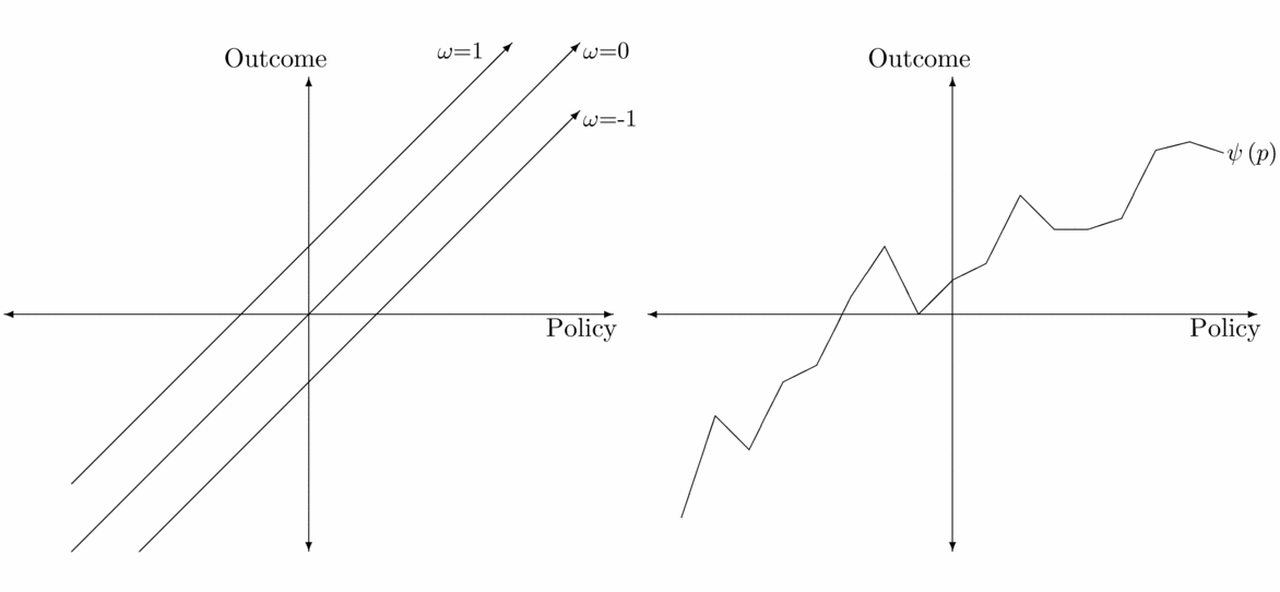
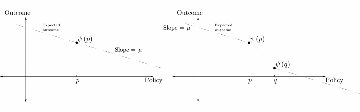
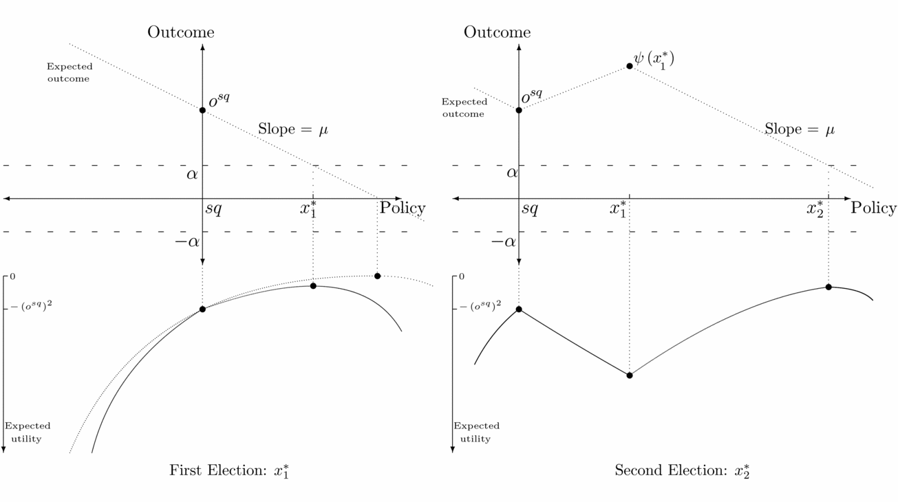
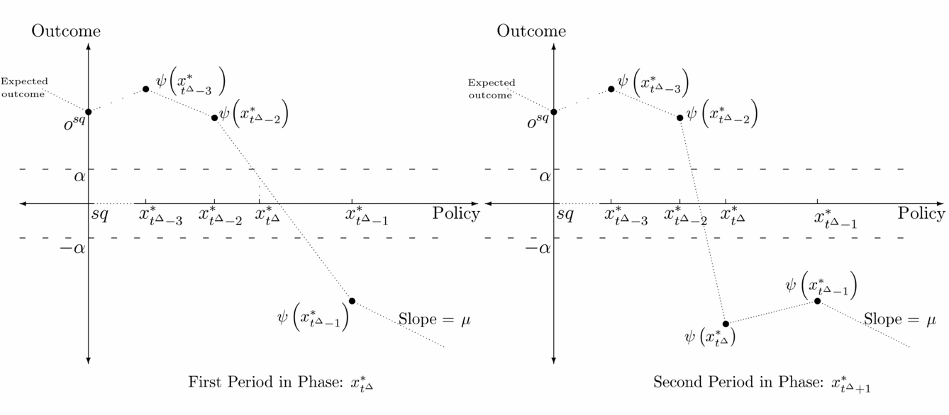
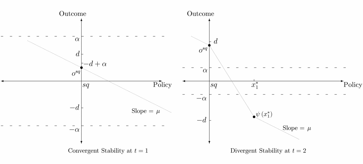



Comments
No Comments have been published for this article.