1 Introduction
Heterogeneity in the hydraulic properties of porous media governs the spreading and mixing of contaminants in subsurface environments (Gelhar & Axness Reference Gelhar and Axness1983; Dagan Reference Dagan1990), and controls the spatial distribution and rates of biogeochemical reactions (Steefel, DePaolo & Lichtner Reference Steefel, DePaolo and Lichtner2005; Dentz et al. Reference Dentz, Le Borgne, Englert and Bijeljic2011). The spatial variability in the porous medium’s hydraulic conductivity induces fluctuations in the Darcy-scale velocity field which in turn causes the solute cloud to distort and spread. As the solute cloud is advected through the heterogeneous porous material, it undergoes a series of shearing and straining motions inherent to the heterogeneous flow field which in turn affect the overall spreading and mixing behaviour of the solute (Gelhar & Axness Reference Gelhar and Axness1983; Dagan Reference Dagan1990; Kitanidis Reference Kitanidis1994; Dentz et al. Reference Dentz, Kinzelbach, Attinger and Kinzelbach2000; Fiori & Dagan Reference Fiori and Dagan2000; Le Borgne et al. Reference Le Borgne, Dentz, Davy, Bolster, Carrera, De Dreuzy and Bour2011; de Barros et al. Reference de Barros, Dentz, Koch and Nowak2012; Le Borgne, Dentz & Villermaux Reference Le Borgne, Dentz and Villermaux2013). While these mechanisms are understood qualitatively, fundamental challenges are to establish a quantitative link between medium heterogeneity, velocity gradients and solute mixing and to quantify the impact of initial solute distribution.
The impact of spatial fluctuations of hydraulic conductivity on solute dispersion has been intensely studied in the literature (e.g. Gelhar & Axness Reference Gelhar and Axness1983; Dagan Reference Dagan1987; Koch & Brady Reference Koch and Brady1987; Neuman Reference Neuman1993; Cushman, Hu & Ginn Reference Cushman, Hu and Ginn1994; Dentz et al. Reference Dentz, Kinzelbach, Attinger and Kinzelbach2000). Dispersion, which quantifies the spatial extent of solute plumes, is not equivalent to mixing, which describes the degree of homogeneity of concentration within the plume (Kitanidis Reference Kitanidis1994; Dentz et al. Reference Dentz, Le Borgne, Englert and Bijeljic2011). Porous media heterogeneity implies that solute plumes can be spatially dispersed and poorly mixed (Le Borgne, Dentz & Villermaux Reference Le Borgne, Dentz and Villermaux2015). Chemical reactions are often controlled by mixing rates rather than dispersion rates (De Simoni et al. Reference De Simoni, Carrera, Sánchez-Vila and Guadagnini2005; Tartakovsky, Tartakovsky & Meakin Reference Tartakovsky, Tartakovsky and Meakin2008; Battiato et al. Reference Battiato, Tartakovsky, Tartakovsky and Scheibe2009; de Anna et al. Reference de Anna, Dentz, Tartakovsky and Le Borgne2014; Engdahl, Benson & Bolster Reference Engdahl, Benson and Bolster2014; Le Borgne, Ginn & Dentz Reference Le Borgne, Ginn and Dentz2014). Solute mixing in porous media has been investigated in terms of effective dispersion coefficients (e.g. Dentz et al. Reference Dentz, Kinzelbach, Attinger and Kinzelbach2000; Fiori & Dagan Reference Fiori and Dagan2000), the decay of concentration variability as measured by the scalar dissipation rate (Kapoor & Kitanidis Reference Kapoor and Kitanidis1998; Le Borgne et al. Reference Le Borgne, Dentz, Bolster, Carrera, de Dreuzy and Davy2010; Bolster et al. Reference Bolster, Valdés-Parada, LeBorgne, Dentz and Carrera2011b ; de Barros et al. Reference de Barros, Fiori, Boso and Bellin2015) and entropy based mixing measures (e.g. Kitanidis Reference Kitanidis1994; de Barros et al. Reference de Barros, Fiori, Boso and Bellin2015). Yet, deriving general mixing laws as a function of porous medium heterogeneity and structure remains an outstanding challenge.
Mixing is enhanced by advective heterogeneity, which leads to fluid stretching and thus to the creation of concentration gradients, and their attenuation due to diffusion or local-scale dispersion. The role of kinematic deformation rates in increasing solute mixing efficiency has been a topic of research in the fluid mechanics community (Batchelor Reference Batchelor1959; Tennekes & Lumley Reference Tennekes and Lumley1972; Ottino Reference Ottino1989; Lapeyre, Klein & Hua Reference Lapeyre, Klein and Hua1999; Duplat & Villermaux Reference Duplat and Villermaux2008). Fluid mixing may be seen as the interplay of stirring, which means stretching and folding of material lines and surfaces, and diffusion. This interplay accelerates scalar dispersion toward the homogeneous limit and so any predictive theory of mixing in fluids must necessarily capture fluid stretching. For two-dimensional unsteady flows (Lester et al. Reference Lester, Rudman, Metcalfe, Trefry, Ord and Hobbs2010) and three-dimensional flow topologies (Ye et al. Reference Ye, Chiogna, Cirpka, Grathwohl and Rolle2015), stretching can be chaotic, which leads to exponential elongations (Lester, Metcalfe & Trefry Reference Lester, Metcalfe and Trefry2013; Lester et al. Reference Lester, Dentz, Le Borgne and de Barros2018) and consequently to fast mixing.
Flows in porous media are particular in that the velocity field (and its structure) is largely dictated by the medium properties rather than the fluid properties and forcing (Bear Reference Bear1972). Weeks & Sposito (Reference Weeks and Sposito1998) analysed fluid stretching in steady and temporally fluctuating groundwater flows. Steady Darcy flows do not admit exponential stretching due to topological constraints imposed by the Darcy equation. Instead, fluid stretching is caused by intermittent shear events, which leads to sub-exponential elongations (Dentz et al.
Reference Dentz, Lester, Borgne and de Barros2016b
; Lester et al.
Reference Lester, Dentz, Le Borgne and de Barros2018). The mechanisms of fluid mixing in heterogeneous porous media can be related to the Okubo–Weiss parameter (de Barros et al.
Reference de Barros, Dentz, Koch and Nowak2012), which quantifies relative strength of fluid rotation to strain (Okubo Reference Okubo1970; Weiss Reference Weiss1991). It is defined as four times the negative determinant of the deformation rate tensor
 $\unicode[STIX]{x1D6E9}=-4\text{det}(\unicode[STIX]{x1D735}\boldsymbol{u}^{\text{T}})$
with
 $\boldsymbol{u}$
the flow velocity, the superscript T denotes the transpose. The impact of fluid deformation on mixing and dilution of a solute blob in the flow through a
 $d=2$
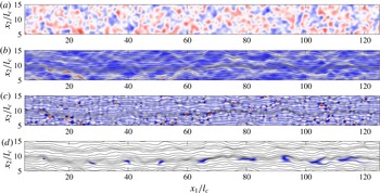
dimensional heterogeneous porous medium are illustrated in figure 1. The two top figures illustrate a realization of a multi-log-normal hydraulic conductivity field (figure 1
a), and the distribution of the absolute values of velocity superposed with the streamlines of the flow (figure 1
b). Regions of low and high velocity are correlated to regions of low and high hydraulic conductivity. The bottom figures show the spatial distribution of the Okubo–Weiss parameter (figure 1
c) as a measure of the flow deformation (Okubo Reference Okubo1970; Weiss Reference Weiss1991), and the evolution of a solute blob (figure 1
d), superposed with the streamlines of the flow field. Negative values of the Okubo–Weiss parameter indicate rotation of a fluid element, positive values indicate strain. Note that a fluid element on the Darcy scale refers to the bulk fluid contained in the saturated porous medium. The bottom figure illustrates the deformation and consequent dilution of the solute blob as it passes through regions of different deformation properties. Strain and rotation of the blob are correlated with the spatial distribution of the Okubo–Weiss parameter (de Barros et al.
Reference de Barros, Dentz, Koch and Nowak2012). Mixing of the solute blob is determined by the shear actions experienced as it travels through regions with different deformation properties, which are delineated by the spatial distribution of the Okubo–Weiss parameter. Following this line of work, Aquino & Bolster (Reference Aquino and Bolster2017) used an analytical–numerical framework to study the impact of shear deformation on the dilution of a point source. These authors represent the deformation action of the flow field in terms of an effective Lagrangian shear deformation, which is defined as the trace of the Lagrangian strain tensor. The latter is determined from direct numerical simulations.
To quantify the effect of fluid stretching in porous media on the enhancement of mixing rates, Villermaux (Reference Villermaux2012) and Le Borgne et al. (Reference Le Borgne, Dentz and Villermaux2013, Reference Le Borgne, Dentz and Villermaux2015) used the diffusive strip method (Duplat & Villermaux Reference Duplat and Villermaux2008; Meunier & Villermaux Reference Meunier and Villermaux2010). This method is based on the picture that the concentration field is stretched into an ensemble of filaments or lamellae by velocity gradients. Since concentration gradients are expected to be small in the direction parallel to lamellae and maximum in the transverse direction, the coupling between stretching and diffusion can be quantified by considering diffusion transverse to lamellae and disregarding longitudinal gradients. While this is consistent for the case of a line injection of solute as considered by Villermaux (Reference Villermaux2012) and Le Borgne et al. (Reference Le Borgne, Dentz and Villermaux2013, Reference Le Borgne, Dentz and Villermaux2015), this model may not apply to cases where diffusive mass transfer occurs with comparable intensity in all directions such as for a solute blob in heterogeneous porous media flows. Furthermore, for porous media flows, the relation between mixing and the underlying medium heterogeneity in the form of the distribution of hydraulic conductivity is still an open question (Dentz et al. Reference Dentz, Lester, Borgne and de Barros2016b ).
In this paper, we address these open issues. Firstly, we derive the governing equations for stretching-enhanced mixing for an arbitrary (finite) initial solute distribution (blob), which may be seen as a generalization of the diffusive strip model. Secondly, using a perturbation theory approach, we relate the stretching and mixing behaviour to the geostatistical characteristics of the underlying medium.
(a) Multi-log-normal hydraulic conductivity field for
 $\unicode[STIX]{x1D70E}_{f}^{2}=1/4$
. The colour scale is logarithmic from red (highest) to blue (lowest value). (b) Spatial distribution of the absolute value of the corresponding Darcy velocity. The colour scale is linear from red (highest) to blue (lowest value). (c) Spatial distribution of the Okubo–Weiss parameter
 $\unicode[STIX]{x1D6E9}(\boldsymbol{x})$
. The colour scale is linear from blue (lowest negative) to red (highest positive value). (d) Snapshots of the solute concentration
 $c(\boldsymbol{x},t)$
evolving from a disk-shaped initial distribution of size
 $\unicode[STIX]{x1D70E}\approx 0.05\ell _{c}$
with
 $\ell _{c}$
the correlation length of the logarithm of hydraulic conductivity, at different times
 $t>\unicode[STIX]{x1D70F}_{u}$
, where
 $\unicode[STIX]{x1D70F}_{u}$
is the characteristic advection time scale. The Péclet number is
 $Pe=5.65\times 10^{2}$
. The solid black lines superposed in (b–d) denote streamlines of the flow field.

The paper is organized as follows. Section 2 introduces the flow and transport problem in Darcy-scale heterogeneous porous media. The mathematical description of diffusion under deformation in streamline coordinates is developed in § 3. Section 4 considers first the evolution of a solute blob in simple shear flow in order to discuss the impact of a finite initial size on the mixing behaviour as quantified in terms of the decay of the maximum concentration. In the second part of § 4, we study solute mixing in a moderately heterogeneous random conductivity field. We determine the deformation and mixing properties using a perturbation approach in the fluctuations of the log-hydraulic conductivity and derive explicit expressions for the resulting solute distribution in terms of the medium properties. In this context, mixing is quantified in terms of the dilution index as a measure for the decay of the maximum concentration in the heterogeneous mixture.
2 Flow and transport
We consider the evolution of a solute blob in a
 $d=2$
dimensional steady incompressible flow field in a fully saturated spatially heterogeneous porous medium free from the influence of boundary conditions. The steady-state velocity field,
 $\boldsymbol{u}(\boldsymbol{x})$
, is determined by the Darcy equation (Bear Reference Bear1972)
 $$\begin{eqnarray}\displaystyle \boldsymbol{u}(\boldsymbol{x})=-K(\boldsymbol{x})\unicode[STIX]{x1D735}h(\boldsymbol{x}), & & \displaystyle\end{eqnarray}$$
where
 $K(\boldsymbol{x})$
is the heterogeneous locally isotropic hydraulic conductivity and
 $h(\boldsymbol{x})$
is the hydraulic head. In this work, the log-conductivity field,
 $f(\boldsymbol{x})=\ln [K(\boldsymbol{x})]$
, is a statistically isotropic random space function characterized by its mean
 $\overline{f}$
, variance
 $\unicode[STIX]{x1D70E}_{f}^{2}$
and correlation scale
 $\ell _{c}$
. The ensemble average over all realizations of
 $K(\boldsymbol{x})$
is denoted by an overbar. The correlation scale is typically of the order of metres or tens of metres (Rubin Reference Rubin2003). In the absence of sinks and sources and under steady-state conditions, the hydraulic head
 $h(\boldsymbol{x})$
is obtained from
 $\unicode[STIX]{x1D735}\boldsymbol{\cdot }\boldsymbol{u}(\boldsymbol{x})=0$
. The average flow velocity is given by
 $\overline{u}=\exp (\overline{f})|\unicode[STIX]{x1D735}\overline{h}(\boldsymbol{x})|$
(Matheron Reference Matheron1968).
Chaotic flow cannot occur in
 $d=2$
dimensional steady flows, this means, the stretching of a fluid element is non-exponential. For three-dimensional flow, the Darcy equation (2.1) implies that the helicity of the flow field
 $\boldsymbol{u}(\boldsymbol{x})$
is zero, which can be seen as follows. The helicity (density) is defined as
 ${\mathcal{H}}=\boldsymbol{u}(\boldsymbol{x})\boldsymbol{\cdot }\unicode[STIX]{x1D74E}(\boldsymbol{x})$
, where
 $\unicode[STIX]{x1D74E}(\boldsymbol{x})=\unicode[STIX]{x1D735}\times \boldsymbol{u}(\boldsymbol{x})$
denotes vorticity. From (2.1), we obtain that vorticity
 $\unicode[STIX]{x1D74E}(\boldsymbol{x})=\unicode[STIX]{x1D735}K(\boldsymbol{x})\times \unicode[STIX]{x1D735}h(\boldsymbol{x})=\unicode[STIX]{x1D735}f(\boldsymbol{x})\times \boldsymbol{u}(\boldsymbol{x})$
. Thus,
 $\unicode[STIX]{x1D74E}(\boldsymbol{x})$
is perpendicular to
 $\boldsymbol{u}(\boldsymbol{x})$
and
 ${\mathcal{H}}(\boldsymbol{x})=0$
. For steady flow fields with helicity 0, this means when
 $\boldsymbol{u}(\boldsymbol{x})$
is perpendicular to its curl, Arnol’d (Reference Arnol’d1966) shows that the streamlines are ‘either closed or everywhere dense on two-dimensional toruses’. This implies that fluid stretching is not exponential. Thus we expect mixing in three-dimensional Darcy flow to be qualitatively similar to Darcy flow in two dimensions. In the following, we focus on
 $d=2$
dimensional porous media.
The spatio-temporal evolution of a passive scalar
 $c(\boldsymbol{x},t)$
in the flow field
 $\boldsymbol{u}(\boldsymbol{x})$
is given by
 $$\begin{eqnarray}\displaystyle \unicode[STIX]{x1D719}\frac{\unicode[STIX]{x2202}c(\boldsymbol{x},t)}{\unicode[STIX]{x2202}t}+\boldsymbol{u}(\boldsymbol{x})\boldsymbol{\cdot }\unicode[STIX]{x1D735}c(\boldsymbol{x},t)-\unicode[STIX]{x1D735}\boldsymbol{\cdot }[\unicode[STIX]{x1D63F}\unicode[STIX]{x1D735}c(\boldsymbol{x},t)]=0, & & \displaystyle\end{eqnarray}$$
where
 $\unicode[STIX]{x1D63F}$
is the (constant) local-scale dispersion tensor;
 $\unicode[STIX]{x1D719}$
is porosity and considered constant here. We set
 $\unicode[STIX]{x1D719}=1$
, which is equivalent to rescaling time. The solute blob is instantaneously released at time
 $t=0$
. The initial blob is represented by the instantaneous injection
 $c(\boldsymbol{x},t=0)=c_{0}(\boldsymbol{x})$
. The advection–dispersion equation (2.2) is equivalent to the Langevin equation (Risken Reference Risken1996)
 $$\begin{eqnarray}\displaystyle \frac{\text{d}\boldsymbol{x}(t;\boldsymbol{a})}{\text{d}t}=\boldsymbol{u}[\boldsymbol{x}(t;\boldsymbol{a})]+\sqrt{2\unicode[STIX]{x1D63F}}\boldsymbol{\cdot }\unicode[STIX]{x1D73B}(t), & & \displaystyle\end{eqnarray}$$
where
 $\unicode[STIX]{x1D73B}(t)$
is a Gaussian white noise of 0 mean and variance
 $\langle \unicode[STIX]{x1D701}_{i}(t)\unicode[STIX]{x1D701}_{j}(t^{\prime })\rangle =\unicode[STIX]{x1D6FF}(t-t^{\prime })$
. The angular brackets denote the noise average. For simplicity, local-scale dispersion is here assumed to be isotropic,
 $D_{ij}=D\unicode[STIX]{x1D6FF}_{ij}$
. The initial positions
 $\boldsymbol{x}(t=0;\boldsymbol{a})=\boldsymbol{a}$
are distributed according to
 $c_{0}(\boldsymbol{x})$
. The relative importance of advective and diffusive mass transfer over the correlation scale
 $\ell _{c}$
is measured by the Péclet number
 $Pe=\overline{u}\ell _{c}/D$
, where
 $\overline{u}$
is a characteristic flow velocity. The Péclet number compares the diffusion time
 $\unicode[STIX]{x1D70F}_{D}=\ell _{c}^{2}/D$
over a correlation length with the characteristic advection time scale
 $\unicode[STIX]{x1D70F}_{u}=\ell _{c}/\overline{u}$
. Groundwater flow and transport is typically advection-dominated with Péclet numbers of the order of
 $10^{2}{-}10^{4}$
(Rubin Reference Rubin2003).
In the following, we solve the flow and transport problems (2.1) and (2.3) numerically and develop an analytical solution for the mixing behaviour in a reference frame that moves along the streamlines of the flow field.
The numerical simulations reported in the following solve the flow problem using a finite difference method with a unit mean hydraulic head gradient across the flow domain and no-flux conditions at the horizontal boundaries. The transport problem is solved using random walk particle tracking based on the discrete version of (2.3) in combination with a bilinear interpolation of flow velocities within finite difference cells to guarantee fluid mass conservation (Pollock Reference Pollock1988). Details of the set-up of the numerical simulations can be found in Le Borgne et al. (Reference Le Borgne, Dentz and Villermaux2013, Reference Le Borgne, Dentz and Villermaux2015).
Figure 1(d) illustrates the evolution of a solute blob in a heterogeneous conductivity field of log-conductivity variance
 $\unicode[STIX]{x1D70E}_{f}^{2}=1/4$
. The initial blob first expands due to diffusion only until it is large enough to experience the impact of velocity heterogeneity, which is characterized by the correlation scale
 $\ell _{c}$
. Then as it migrates through the medium, it experiences different stretching regimes and elongates in direction of the mean flow mainly as a consequence of velocity contrasts perpendicular to the streamlines.
In the following, we quantify this evolution by transforming the transport problem into a set of streamline coordinates, which comprise a rectilinear coordinate system attached to a fluid element, whose coordinate axes rotate according to the streamline orientation. Note that a fluid element on the Darcy scale refers to a bulk fluid volume that contains both fluid and porous material. We first formulate the evolution of a solute blob under the influence of diffusion and flow deformation. Then we consider the blob evolution under simple shear flow and in a moderately heterogeneous hydraulic conductivity field, this means with a variance of log-hydraulic conductivity smaller than 1. The evolution of mixing is measured in terms of the maximum concentration
 $c_{m}(t)$
, or the characteristic volume occupied by the solute. For a heterogeneous mixture, we consider the dilution index (Kitanidis Reference Kitanidis1994)
 $$\begin{eqnarray}\displaystyle E(t)=\exp [H(t)], & & \displaystyle\end{eqnarray}$$
where
 $H(t)$
is the entropy of the mixture
 $$\begin{eqnarray}\displaystyle H(t)=-\int \text{d}\boldsymbol{x}c(\boldsymbol{x},t)\ln [c(\boldsymbol{x},t)]. & & \displaystyle\end{eqnarray}$$
The dilution index is a measure for the volume occupied by the scalar and its inverse can be seen as a measure for the maximum concentration in the mixture. For a Gaussian-shaped solute distribution, the dilution index is in fact
 $$\begin{eqnarray}\displaystyle E(t)=\frac{e}{c_{m}(t)}. & & \displaystyle\end{eqnarray}$$
3 Diffusion under flow deformation
In this section, we formulate the evolution of a solute blob under the action of diffusion and flow deformation in
 $d=2$
dimensional steady flow.
3.1 Flow deformation along streamlines
We first consider the equation of motion of a fluid particle. The particle position
 $\boldsymbol{x}_{f}(t;\boldsymbol{a})$
evolves according to the advection equation
 $$\begin{eqnarray}\displaystyle \frac{\text{d}\boldsymbol{x}_{f}(t;\boldsymbol{a})}{\text{d}t}=\boldsymbol{v}(t), & & \displaystyle\end{eqnarray}$$
with the initial condition
 $\boldsymbol{x}_{f}(t=0;\boldsymbol{a})=\boldsymbol{a}$
. The Lagrangian velocity is given by
 $\boldsymbol{v}(t)=\boldsymbol{u}[\boldsymbol{x}_{f}(t;\boldsymbol{a})]$
. The velocity magnitude along the streamline is denoted by
 $v(t)=|\boldsymbol{v}(t)|$
and the velocity magnitude at a given distance
 $s$
along the streamline is
 $v_{s}(s)=v[t(s)]$
with (Dentz et al.
Reference Dentz, Kang, Comolli, Le Borgne and Lester2016a
)
 $$\begin{eqnarray}\displaystyle \frac{\text{d}s(t)}{\text{d}t}=v(t),\quad \frac{\text{d}t(s)}{\text{d}s}=\frac{1}{v_{s}(s)}. & & \displaystyle\end{eqnarray}$$
The deformation properties of the flow field are quantified by considering the evolution of a fluid material element whose length and orientation are defined by
 $$\begin{eqnarray}\displaystyle \boldsymbol{z}(t)=\boldsymbol{x}_{f}(t;\boldsymbol{a}+\unicode[STIX]{x1D6FF}\boldsymbol{a})-\boldsymbol{x}_{f}(t;\boldsymbol{a}). & & \displaystyle\end{eqnarray}$$
The temporal change of the vector
 $\boldsymbol{z}(t)$
is
 $$\begin{eqnarray}\displaystyle \frac{\text{d}\boldsymbol{z}(t)}{\text{d}t}=\unicode[STIX]{x1D750}(t)\boldsymbol{z}(t)+\cdots \,, & & \displaystyle\end{eqnarray}$$
where the dots indicate contributions of order
 $|\boldsymbol{z}(t)|^{2}$
. The deformation rate tensor is given by
 $$\begin{eqnarray}\displaystyle \unicode[STIX]{x1D750}(t)=\unicode[STIX]{x1D735}\boldsymbol{v}[\boldsymbol{x}_{f}(t;\boldsymbol{a})]^{\text{T}}. & & \displaystyle\end{eqnarray}$$
Note that
 $\unicode[STIX]{x1D716}_{11}(t)=-\unicode[STIX]{x1D716}_{22}(t)$
because of
 $\unicode[STIX]{x1D735}\boldsymbol{\cdot }\boldsymbol{u}(\boldsymbol{x})=0$
. We transform the deformation problem into the coordinate system
 $\boldsymbol{x}^{\prime }(t)$
moving with
 $\boldsymbol{x}_{f}(t;\boldsymbol{a})$
via the linear transform
 $$\begin{eqnarray}\displaystyle \boldsymbol{x}^{\prime }=\unicode[STIX]{x1D63C}^{\text{T}}(t)[\boldsymbol{x}-\boldsymbol{x}_{f}(t;\boldsymbol{a})], & & \displaystyle\end{eqnarray}$$
where
 $\boldsymbol{x}$
and
 $\boldsymbol{x}^{\prime }$
are coordinate vectors in the fixed and moving coordinate systems, respectively;
 $\unicode[STIX]{x1D63C}(t)$
is a time-dependent orthogonal matrix and
 $\unicode[STIX]{x1D63C}^{\text{T}}(t)$
its transpose such that
 $$\begin{eqnarray}\displaystyle \unicode[STIX]{x1D63C}(t)\unicode[STIX]{x1D63C}^{\text{T}}(t)=\unicode[STIX]{x1D63C}^{\text{T}}(t)\unicode[STIX]{x1D63C}(t)=1. & & \displaystyle\end{eqnarray}$$
The columns of the transformation matrix are equal to the unit vectors of the new coordinate system,
 $\unicode[STIX]{x1D63C}(t)=[\boldsymbol{e}_{1}^{\prime }(t),\boldsymbol{e}_{2}^{\prime }(t)]$
. The displacement vector
 $\boldsymbol{z}(t)$
transforms as
 $$\begin{eqnarray}\displaystyle \boldsymbol{z}^{\prime }(t)=\unicode[STIX]{x1D63C}^{\text{T}}(t)\boldsymbol{z}(t). & & \displaystyle\end{eqnarray}$$
From this, we obtain for the deformation
 $$\begin{eqnarray}\displaystyle \frac{\text{d}\boldsymbol{z}^{\prime }(t)}{\text{d}t}=[\unicode[STIX]{x1D64C}+\unicode[STIX]{x1D63C}^{\text{T}}(t)\unicode[STIX]{x1D750}(t)\unicode[STIX]{x1D63C}(t)]\boldsymbol{z}^{\prime }(t), & & \displaystyle\end{eqnarray}$$
where we defined the antisymmetric tensor
 $$\begin{eqnarray}\displaystyle \unicode[STIX]{x1D64C}=\frac{\text{d}\unicode[STIX]{x1D63C}^{\text{T}}(t)}{\text{d}t}\unicode[STIX]{x1D63C}(t), & & \displaystyle\end{eqnarray}$$
see also Ottino (Reference Ottino1989). The antisymmetry can be seen as follows
 $$\begin{eqnarray}\displaystyle \frac{\text{d}}{\text{d}t}[\unicode[STIX]{x1D63C}^{\text{T}}(t)\unicode[STIX]{x1D63C}(t)]=\frac{\text{d}\unicode[STIX]{x1D63C}^{\text{T}}(t)}{\text{d}t}\unicode[STIX]{x1D63C}(t)+\frac{\text{d}\unicode[STIX]{x1D63C}(t)}{\text{d}t}\unicode[STIX]{x1D63C}^{\text{T}}(t)=0. & & \displaystyle\end{eqnarray}$$
From (3.9), we find that the velocity gradient transforms as
 $$\begin{eqnarray}\displaystyle \unicode[STIX]{x1D750}^{\prime }(t)=\unicode[STIX]{x1D64C}+\unicode[STIX]{x1D63C}^{\text{T}}(t)\unicode[STIX]{x1D750}(t)\unicode[STIX]{x1D63C}(t), & & \displaystyle\end{eqnarray}$$
which makes it a pseudo-tensor (Ottino Reference Ottino1989) because the transform of
 $\unicode[STIX]{x1D750}(t)$
by
 $\unicode[STIX]{x1D63C}(t)$
is
 $\tilde{\unicode[STIX]{x1D750}}(t)=\unicode[STIX]{x1D63C}^{\text{T}}(t)\unicode[STIX]{x1D750}(t)\unicode[STIX]{x1D63C}(t)$
. The matrix
 $\unicode[STIX]{x1D64C}$
can also be written as
 $$\begin{eqnarray}\displaystyle \unicode[STIX]{x1D64C}(t)=\left[\begin{array}{@{}cc@{}}0 & \displaystyle \boldsymbol{e}_{2}^{\prime }(t)\boldsymbol{\cdot }{\displaystyle \frac{\text{d}\boldsymbol{e}_{1}^{\prime }(t)}{\text{d}t}}\\ -\boldsymbol{e}_{2}^{\prime }(t)\boldsymbol{\cdot }{\displaystyle \frac{\text{d}\boldsymbol{e}_{1}^{\prime }(t)}{\text{d}t}} & \displaystyle 0\end{array}\right]. & & \displaystyle\end{eqnarray}$$
In the following, we consider flow deformation and blob evolution in the streamline coordinate system, whose 1-axis is aligned with
 $\boldsymbol{v}(t)$
. This transformation allows us to elucidate the deformation structure of the flow while enforcing topological constraints associated with
 $d=2$
dimensional steady flow (Dentz et al.
Reference Dentz, Lester, Borgne and de Barros2016b
; Lester et al.
Reference Lester, Dentz, Le Borgne and de Barros2018). The deformation evolution (3.4) tends to produce exponential stretching solutions. Note that for diagonal and constant
 $\unicode[STIX]{x1D750}$
with
 $\unicode[STIX]{x1D716}_{11}=-\unicode[STIX]{x1D716}_{22}>0$
it implies exponential growth for
 $z_{1}(t)$
and thus for
 $z(t)=|\boldsymbol{z}(t)|$
.
In
 $d=2$
dimensional steady flows, on the other hand, deformation is constrained to algebraic stretching as outlined in the following. The use of streamline coordinates allows to naturally recover this constraint. The unit vectors in the new coordinate system are
 $\boldsymbol{e}_{1}^{\prime }(t)=[v_{1}(t),v_{2}(t)]^{\text{T}}/v(t)$
, which is tangential, and
 $\boldsymbol{e}_{2}^{\prime }(t)=[-v_{2}(t),v_{1}(t)]^{\text{T}}/v(t)$
, which is normal to the streamline. The transformation matrix
 $\unicode[STIX]{x1D63C}(t)$
in the streamline coordinate system is
 $$\begin{eqnarray}\displaystyle \unicode[STIX]{x1D63C}(t)=\frac{1}{v(t)}\left[\begin{array}{@{}cc@{}}v_{1}(t) & \displaystyle -v_{2}(t)\\ v_{2}(t) & \displaystyle v_{1}(t)\end{array}\right]. & & \displaystyle\end{eqnarray}$$
The derivative of
 $\boldsymbol{e}_{1}^{\prime }(t)$
with respect to time is
 $$\begin{eqnarray}\displaystyle \frac{\text{d}\boldsymbol{e}_{1}^{\prime }(t)}{\text{d}t}=-\frac{1}{v(t)}\frac{\text{d}v(t)}{\text{d}t}\boldsymbol{e}_{1}^{\prime }(t)+\unicode[STIX]{x1D750}(t)\boldsymbol{e}_{1}^{\prime }(t) & & \displaystyle\end{eqnarray}$$
and therefore
 $$\begin{eqnarray}\displaystyle \boldsymbol{e}_{2}^{\prime }(t)\boldsymbol{\cdot }\frac{\text{d}\boldsymbol{e}_{1}^{\prime }(t)}{\text{d}t}=\boldsymbol{e}_{2}^{\prime }(t)\boldsymbol{\cdot }\unicode[STIX]{x1D750}(t)\boldsymbol{e}_{1}^{\prime }(t)=\tilde{\unicode[STIX]{x1D716}}_{21}(t). & & \displaystyle\end{eqnarray}$$
Thus,
 $\unicode[STIX]{x1D64C}(t)$
defined by (3.13) reads as
 $$\begin{eqnarray}\displaystyle \unicode[STIX]{x1D64C}(t)=\left[\begin{array}{@{}cc@{}}0 & \displaystyle \tilde{\unicode[STIX]{x1D716}}_{21}(t)\\ -\tilde{\unicode[STIX]{x1D716}}_{21}(t) & \displaystyle 0\end{array}\right]. & & \displaystyle\end{eqnarray}$$
As a result, we obtain for the deformation tensor in the moving coordinate system the upper triangular form
 $$\begin{eqnarray}\displaystyle \unicode[STIX]{x1D750}^{\prime }(t)=\left(\begin{array}{@{}cc@{}}\unicode[STIX]{x1D6FC}^{\prime }(t) & \displaystyle \unicode[STIX]{x1D6FE}^{\prime }(t)\\ 0 & \displaystyle -\unicode[STIX]{x1D6FC}^{\prime }(t)\end{array}\right), & & \displaystyle\end{eqnarray}$$
with
 $$\begin{eqnarray}\displaystyle & \displaystyle \unicode[STIX]{x1D6FE}^{\prime }(t)=\tilde{\unicode[STIX]{x1D716}}_{12}(t)+\tilde{\unicode[STIX]{x1D716}}_{21}(t), & \displaystyle\end{eqnarray}$$
 $$\begin{eqnarray}\displaystyle & \displaystyle \unicode[STIX]{x1D6FC}^{\prime }(t)=\frac{1}{v(t)}\frac{\text{d}v(t)}{\text{d}t}. & \displaystyle\end{eqnarray}$$
Note that
 $\unicode[STIX]{x1D6FC}^{\prime }(t)$
represents fluid stretching and compression due to fluctuations of the streamwise velocity magnitude, while
 $\unicode[STIX]{x1D6FE}^{\prime }(t)$
represents such due to curvature of the streamline and the transverse velocity gradient. The triangular form is a consequence of the steadiness of the flow field. The evolution of the material strip
 $\boldsymbol{z}^{\prime }(t)$
is given by using (3.18) in (3.9) as
 $$\begin{eqnarray}\displaystyle & \displaystyle \frac{\text{d}z_{1}^{\prime }(t)}{\text{d}t}=\frac{1}{v(t)}\frac{\text{d}v(t)}{\text{d}t}z_{1}^{\prime }(t)+\unicode[STIX]{x1D6FE}^{\prime }(t)z_{2}^{\prime }(t), & \displaystyle\end{eqnarray}$$
 $$\begin{eqnarray}\displaystyle & \displaystyle \frac{\text{d}z_{2}^{\prime }(t)}{\text{d}t}=-\frac{1}{v(t)}\frac{\text{d}v(t)}{\text{d}t}z_{2}^{\prime }(t). & \displaystyle\end{eqnarray}$$
Its solution is obtained by separation of variables as (Dentz et al. Reference Dentz, Lester, Borgne and de Barros2016b )
 $$\begin{eqnarray}\displaystyle & \displaystyle z_{1}^{\prime }(t)=z_{1}(0)\frac{v(t)}{v(0)}+z_{2}(0)v(t)\int _{0}^{t}\,\text{d}t^{\prime }\frac{v(0)\unicode[STIX]{x1D6FE}^{\prime }(t^{\prime })}{v(t^{\prime })^{2}}, & \displaystyle\end{eqnarray}$$
 $$\begin{eqnarray}\displaystyle & \displaystyle z_{2}^{\prime }(t)=z_{2}(0)\frac{v(0)}{v(t)}. & \displaystyle\end{eqnarray}$$
Deformation along the streamline has no net effect on deformation. This can be seen by setting
 $z_{2}(0)=0$
. In this case,
 $z_{2}(t)\equiv 0$
and
 $z_{1}(t)$
fluctuates in the same way as the streamwise velocity magnitude. The only persistent stretching mechanism is due to shear as expressed by the second term in (3.23). It gives rise to algebraic and sub-exponential stretching, which is determined by the flow statistics (Dentz et al.
Reference Dentz, Lester, Borgne and de Barros2016b
).
3.2 Diffusion along streamlines
Diffusive particle motion is described by the Langevin equation (2.3) for
 $D_{ij}=D\unicode[STIX]{x1D6FF}_{ij}$
as
 $$\begin{eqnarray}\displaystyle \frac{\text{d}\boldsymbol{x}(t;\boldsymbol{a})}{\text{d}t}=\boldsymbol{u}[\boldsymbol{x}(t;\boldsymbol{a})]+\sqrt{2D}\unicode[STIX]{x1D743}(t), & & \displaystyle\end{eqnarray}$$
where
 $\unicode[STIX]{x1D743}(t)$
is a Gaussian white noise with
 $\langle \unicode[STIX]{x1D709}_{i}(t)\unicode[STIX]{x1D709}_{j}(t^{\prime })\rangle =\unicode[STIX]{x1D6FF}_{ij}\unicode[STIX]{x1D6FF}(t-t^{\prime })$
. In order to study stretching-enhanced diffusion in this framework, we perform a variable transformation into the coordinate system moving with the fluid support located at
 $\boldsymbol{x}_{f}(t;\boldsymbol{a})$
considered in the previous section. This means
 $\boldsymbol{x}^{\prime \prime }(t)=\boldsymbol{x}(t;\boldsymbol{a})-\boldsymbol{x}_{f}(t;\boldsymbol{a})$
, which gives
 $$\begin{eqnarray}\displaystyle \frac{\text{d}\boldsymbol{x}^{\prime \prime }(t)}{\text{d}t}=\unicode[STIX]{x1D750}(t)\boldsymbol{x}^{\prime \prime }(t)+\sqrt{2D}\unicode[STIX]{x1D743}(t), & & \displaystyle\end{eqnarray}$$
where we used (3.1). Notice that this approximation is strictly valid as long as
 $|\boldsymbol{x}^{\prime \prime }(t)|<\ell _{c}$
, where
 $\ell _{c}$
is a characteristic variation scale of the velocity field
 $\boldsymbol{u}(\boldsymbol{x})$
(de Barros et al.
Reference de Barros, Dentz, Koch and Nowak2012). Rotation following the streamline orientation according to (3.6), this means
 $\boldsymbol{x}^{\prime }(t)=\unicode[STIX]{x1D63C}^{\text{T}}\boldsymbol{x}^{\prime \prime }(t)$
gives
 $$\begin{eqnarray}\displaystyle & \displaystyle \frac{\text{d}x_{1}^{\prime }(t)}{\text{d}t}=\unicode[STIX]{x1D6FC}^{\prime }(t)x_{1}^{\prime }(t)+\unicode[STIX]{x1D6FE}(t)x_{2}^{\prime }(t)+\sqrt{2D}\unicode[STIX]{x1D709}_{1}(t), & \displaystyle\end{eqnarray}$$
 $$\begin{eqnarray}\displaystyle & \displaystyle \frac{\text{d}x_{2}^{\prime }(t)}{\text{d}t}=-\unicode[STIX]{x1D6FC}^{\prime }(t)x_{2}^{\prime }(t)+\sqrt{2D}\unicode[STIX]{x1D709}_{2}(t). & \displaystyle\end{eqnarray}$$
In order to determine the behaviour of diffusion under deformation, we consider the Fokker–Planck equation that describes the evolution of the solute distribution in the coordinate system moving with a fluid particle along a streamline as (Risken Reference Risken1996)
 $$\begin{eqnarray}\frac{\unicode[STIX]{x2202}c(\boldsymbol{x},t)}{\unicode[STIX]{x2202}t}+[\unicode[STIX]{x1D6FC}(t)x_{1}+\unicode[STIX]{x1D6FE}(t)x_{2}]\frac{\unicode[STIX]{x2202}c(\boldsymbol{x},t)}{\unicode[STIX]{x2202}x_{1}}-\unicode[STIX]{x1D6FC}(t)x_{2}\frac{\unicode[STIX]{x2202}c(\boldsymbol{x},t)}{\unicode[STIX]{x2202}x_{2}}-D\unicode[STIX]{x1D6FB}^{2}c(\boldsymbol{x},t)=0,\end{eqnarray}$$
where the advection terms of (3.27) are used. Equation (3.28) describes the spatio-temporal evolution of a solute blob in the streamline coordinate system. The evolution of the blob concentration is directly linked to the deformation properties of the flow field through
 $\unicode[STIX]{x1D6FC}(t)$
and
 $\unicode[STIX]{x1D6FE}(t)$
. This equation can be solved exactly by Fourier transformation and subsequent integration along the characteristics of the transformed equation (Risken Reference Risken1996), see also appendix A. We consider a normalized Gaussian initial distribution characterized by the variance matrix
 $\unicode[STIX]{x1D748}$
. Thus, we obtain the following exact solution for the evolution of the blob concentration
 $c(\boldsymbol{x},t)$
 $$\begin{eqnarray}\displaystyle c(\boldsymbol{x},t)=\frac{\exp \left[-\boldsymbol{x}\unicode[STIX]{x1D73F}^{-1}(t)\boldsymbol{x}/2\right]}{2\unicode[STIX]{x03C0}\sqrt{\text{det}[\unicode[STIX]{x1D73F}(t)]}}, & & \displaystyle\end{eqnarray}$$
where
 $\unicode[STIX]{x1D73F}^{-1}(t)$
is the inverse of the covariance matrix
 $\unicode[STIX]{x1D73F}(t)$
,
 $$\begin{eqnarray}\displaystyle \unicode[STIX]{x1D73F}(t)=2D\unicode[STIX]{x1D726}(t)+\unicode[STIX]{x1D71F}(t). & & \displaystyle\end{eqnarray}$$
The matrix
 $\unicode[STIX]{x1D726}(t)$
represents the growth of the variance due to diffusion enhanced by deformation. It is defined by its coefficients as
 $$\begin{eqnarray}\displaystyle \unicode[STIX]{x1D6EC}_{11}(t) & = & \displaystyle \frac{v(t)^{2}}{v(0)^{2}}\int _{0}^{t}\,\text{d}t^{\prime }\left[\frac{v(0)^{2}}{v(t^{\prime })^{2}}+\frac{v(t^{\prime })^{2}}{v(0)^{2}}r(t^{\prime })^{2}\right]+\frac{v(t)^{2}}{v(0)^{2}}r(t)^{2}w(t)\nonumber\\ \displaystyle & & \displaystyle -\,2\frac{r(t)v(t)^{2}}{v(0)^{2}}\int _{0}^{t}\,\text{d}t^{\prime }\frac{v(t^{\prime })^{2}r(t^{\prime })}{v(0)^{2}},\end{eqnarray}$$
 $$\begin{eqnarray}\unicode[STIX]{x1D6EC}_{12}(t)=\unicode[STIX]{x1D6EC}_{21}(t)=-\int _{0}^{t}\,\text{d}t^{\prime }\frac{v(t^{\prime })^{2}r(t^{\prime })}{v(0)^{2}}+r(t)w(t),\end{eqnarray}$$
 $$\begin{eqnarray}\unicode[STIX]{x1D6EC}_{22}(t)=\frac{v(0)^{2}}{v(t)^{2}}w(t).\end{eqnarray}$$
We defined for compactness
 $$\begin{eqnarray}\displaystyle w(t)=\int _{0}^{t}\,\text{d}t^{\prime }\frac{v(t^{\prime })^{2}}{v(0)^{2}},\quad r(t)=\int _{0}^{t}\,\text{d}t^{\prime }\unicode[STIX]{x1D6FE}(t^{\prime })\frac{v(0)^{2}}{v(t^{\prime })^{2}}. & & \displaystyle\end{eqnarray}$$
The matrix
 $\unicode[STIX]{x1D71F}(t)$
represents the contribution to the variance from purely kinematic deformation of the initial distribution
 $c_{0}(\boldsymbol{x})$
. It is defined by its components as
 $$\begin{eqnarray}\displaystyle \unicode[STIX]{x1D6E5}_{11}(t) & = & \displaystyle \frac{v(t)^{2}}{v(0)^{2}}\unicode[STIX]{x1D70E}_{11}^{2}+r(t)^{2}\unicode[STIX]{x1D70E}_{22}^{2}+2\frac{v(t)}{v(0)}r(t)\unicode[STIX]{x1D70E}_{12}^{2},\end{eqnarray}$$
 $$\begin{eqnarray}\displaystyle \unicode[STIX]{x1D6E5}_{12}(t) & = & \displaystyle \unicode[STIX]{x1D6E5}_{21}(t)=\unicode[STIX]{x1D70E}_{12}^{2}+\frac{v(0)}{v(t)}r(t)\unicode[STIX]{x1D70E}_{22}^{2},\end{eqnarray}$$
 $$\begin{eqnarray}\displaystyle \unicode[STIX]{x1D6E5}_{22}(t) & = & \displaystyle \frac{v(0)^{2}}{v(t)^{2}}\unicode[STIX]{x1D70E}_{22}^{2},\end{eqnarray}$$
 $\unicode[STIX]{x1D70E}_{12}^{2}=\unicode[STIX]{x1D70E}_{21}^{2}$
. The covariance tensor
 $\unicode[STIX]{x1D73F}(t)$
contains all the information on the action of diffusion and flow deformation on the blob evolution. From (3.29) we obtain directly the maximum concentration as
 $$\begin{eqnarray}\displaystyle c_{m}(t)=\frac{1}{2\unicode[STIX]{x03C0}\sqrt{\text{det}[\unicode[STIX]{x1D73F}(t)]}}. & & \displaystyle\end{eqnarray}$$
Information on the evolution of the maximum concentration is of fundamental importance in applications related to contaminant site management (de Barros et al. Reference de Barros, Fernàndez-Garcia, Bolster and Sanchez-Vila2013) and risk analysis (de Barros & Rubin Reference de Barros and Rubin2008; Henri, Fernàndez-Garcia & Barros Reference Henri, Fernàndez-Garcia and Barros2015). It can also serve as a proxy for the dilution of the solute blob. In fact, the dilution index (Kitanidis Reference Kitanidis1994) is given accordingly in terms of the inverse of the maximum concentration
 $$\begin{eqnarray}\displaystyle E(t)=2\unicode[STIX]{x03C0}e\sqrt{\text{det}[\unicode[STIX]{x1D73F}(t)]}. & & \displaystyle\end{eqnarray}$$
The determinant of the variance matrix
 $\unicode[STIX]{x1D73F}(t)$
is given by
 $$\begin{eqnarray}\text{det}[\unicode[STIX]{x1D73F}(t)]=[2D\unicode[STIX]{x1D6EC}_{11}(t)+\unicode[STIX]{x1D6E5}_{11}(t)][2D\unicode[STIX]{x1D6EC}_{22}(t)+\unicode[STIX]{x1D6E5}_{22}(t)]-[2D\unicode[STIX]{x1D6EC}_{12}(t)+\unicode[STIX]{x1D6E5}_{12}(t)]^{2}.\end{eqnarray}$$
The developed framework for the evolution of a solute blob can be used for the determination of the concentration content of the plume because it provides an estimate of the concentration distribution under the action of flow deformation and diffusion through equation (3.29). Thus, it can form the basis for the calculation of the probability density function of concentration within and between realizations of the porous medium in the stretching-dominated mixing regime following the approaches of Villermaux (Reference Villermaux2012) and Le Borgne et al. (Reference Le Borgne, Dentz and Villermaux2015). In the following, we study the blob evolution in terms of the maximum concentration as a result of diffusion and fluid deformation.
4 Blob evolution
We employ the results derived in the previous section for the quantification of the evolution of a solute blob in simple shear flow as well as flows in a moderately heterogeneous porous medium, i.e. with a variance of log-hydraulic conductivity smaller than
 $1$
. For the latter case, we employ stochastic perturbation theory to directly relate the medium and Eulerian flow properties to fluid deformation and thus solute mixing.
4.1 Simple shear flow
We first consider the case of a simple shear flow. The flow field is given by
 $$\begin{eqnarray}\displaystyle \boldsymbol{u}(\boldsymbol{x})=\boldsymbol{e}_{1}\unicode[STIX]{x1D6FE}x_{2}, & & \displaystyle\end{eqnarray}$$
where
 $\unicode[STIX]{x1D6FE}$
is the constant shear rate. These type of flows can be found for variable density flows in the limit of low Péclet numbers (Dentz et al.
Reference Dentz, Tartakovsky, Abarca, Guadagnini and Carrera2006), and flow in sedimentary formations, for which the horizontal correlation length is much longer than the vertical (Matheron & de Marsily Reference Matheron and de Marsily1980). The specific form (4.1) implies that the Lagrangian velocity magnitude
 $v(t)=v(0)$
and shear rate
 $\unicode[STIX]{x1D6FE}(t)=\unicode[STIX]{x1D6FE}(0)$
in (3.31) are constant. Thus,
 $r(t)$
defined by (3.32) and
 $w(t)$
defined by (3.32) reduce to
 $$\begin{eqnarray}\displaystyle r(t)=\unicode[STIX]{x1D6FE}t,\quad \displaystyle w(t)=t. & & \displaystyle\end{eqnarray}$$
We consider now the case
 $\unicode[STIX]{x1D70E}_{12}^{2}=\unicode[STIX]{x1D70E}_{21}^{2}=0$
so that the initial blob is characterized by its variances
 $\unicode[STIX]{x1D70E}_{11}$
and
 $\unicode[STIX]{x1D70E}_{22}$
, respectively parallel and perpendicular to the flow direction. The characteristic time scales are the time for diffusion over the distance
 $\unicode[STIX]{x1D70E}_{22}$
and the characteristic shear time scale, which are defined by
 $$\begin{eqnarray}\displaystyle \unicode[STIX]{x1D70F}_{\unicode[STIX]{x1D70E}}=\frac{\unicode[STIX]{x1D70E}_{22}^{2}}{D},\quad \unicode[STIX]{x1D70F}_{\unicode[STIX]{x1D6FE}}=\unicode[STIX]{x1D6FE}^{-1}, & & \displaystyle\end{eqnarray}$$
respectively. In the following, we non-dimensionalize time with the diffusion time such that
 $t=\hat{t}\unicode[STIX]{x1D70F}_{\unicode[STIX]{x1D70E}}$
and distance by
 $\unicode[STIX]{x1D70E}_{22}$
. Thus, we define the dimensionless variance
 $\hat{\unicode[STIX]{x1D705}}_{ij}(t)$
, shear rate
 $\hat{\unicode[STIX]{x1D6FE}}$
and shear time scale
 $\hat{\unicode[STIX]{x1D70F}}_{\unicode[STIX]{x1D6FE}}$
 $$\begin{eqnarray}\unicode[STIX]{x1D705}_{ij}(t)=\hat{\unicode[STIX]{x1D705}}_{ij}(\hat{t}\unicode[STIX]{x1D70F}_{\unicode[STIX]{x1D70E}})\unicode[STIX]{x1D70E}_{22}^{2},\quad \unicode[STIX]{x1D6FE}=\hat{\unicode[STIX]{x1D6FE}}/\unicode[STIX]{x1D70F}_{\unicode[STIX]{x1D70E}},\quad \unicode[STIX]{x1D70F}_{\unicode[STIX]{x1D6FE}}=\hat{\unicode[STIX]{x1D70F}}_{\unicode[STIX]{x1D6FE}}\unicode[STIX]{x1D70F}_{\unicode[STIX]{x1D70E}}.\end{eqnarray}$$
Note that the non-dimensional shear rate
 $\hat{\unicode[STIX]{x1D6FE}}=\unicode[STIX]{x1D6FE}\unicode[STIX]{x1D70E}_{22}^{2}/D\equiv Pe_{\unicode[STIX]{x1D6FE}}$
defines a Péclet number in that it compares the time scales for shear action and diffusion over the initial blob size perpendicular to the flow direction. This non-dimensionalization implies that the dimensionless shear time scale is
 $\hat{\unicode[STIX]{x1D70F}}_{\unicode[STIX]{x1D6FE}}=Pe_{\unicode[STIX]{x1D6FE}}^{-1}$
. The diffusion time scale across
 $\unicode[STIX]{x1D70E}_{22}$
is naturally unity. The diffusion time scale across
 $\unicode[STIX]{x1D70E}_{11}$
is equal to
 $\hat{\unicode[STIX]{x1D70E}}_{11}$
.
In the following, we drop the hats for simplicity of notation. Using this non-dimensionalization in (3.31) and (3.33) and setting
 $\unicode[STIX]{x1D70E}_{12}=\unicode[STIX]{x1D70E}_{21}=0$
, we obtain for the spatial variance tensor
 $$\begin{eqnarray}\displaystyle \unicode[STIX]{x1D705}_{11}(t) & = & \displaystyle 2t+\frac{2\unicode[STIX]{x1D6FE}^{2}t^{3}}{3}+\unicode[STIX]{x1D70E}_{11}^{2}+\unicode[STIX]{x1D6FE}^{2}t^{2},\end{eqnarray}$$
 $$\begin{eqnarray}\displaystyle \unicode[STIX]{x1D705}_{12}(t) & = & \displaystyle \unicode[STIX]{x1D6FE}t^{2}+\unicode[STIX]{x1D6FE}t,\end{eqnarray}$$
 $$\begin{eqnarray}\displaystyle \unicode[STIX]{x1D705}_{22}(t) & = & \displaystyle 2t+1.\end{eqnarray}$$
 $\unicode[STIX]{x1D6FC}(t)=0$
(Okubo Reference Okubo1968; Bolster, Dentz & Le Borgne Reference Bolster, Dentz and Le Borgne2011a
) and non-dimensionalization according to (4.4). Thus, the maximum concentration in the blob is given by
 $$\begin{eqnarray}\displaystyle c_{m}(t)=\frac{\sqrt{3}}{2\unicode[STIX]{x03C0}}[(t^{4}+2t^{3})\unicode[STIX]{x1D6FE}^{2}+12t^{2}+6t(\unicode[STIX]{x1D70E}_{11}^{2}+1)+3\unicode[STIX]{x1D70E}_{11}^{2}]^{-1/2}. & & \displaystyle\end{eqnarray}$$
For illustration, we consider in the following three different scenarios, which correspond to the deformation of an elongated lamella-like initial blob, a strongly sheared and a weakly sheared symmetric initial blob.
The case of an elongated lamella-like elliptic blob is characterized by
 $\unicode[STIX]{x1D70E}_{11}^{2}\ll 1$
and
 $Pe_{\unicode[STIX]{x1D6FE}}=10^{2}$
. For this scenario, the shear time scale is much smaller than the characteristic diffusion time,
 $\unicode[STIX]{x1D70F}_{\unicode[STIX]{x1D6FE}}=Pe_{\unicode[STIX]{x1D6FE}}^{-1}\ll 1$
. We observe four different time regimes for
 $c_{m}(t)$
as illustrated in figure 2. For times
 $t\ll \unicode[STIX]{x1D70E}_{11}^{2}$
the maximum concentration is constant, given essentially by the initial concentration value. Then it decays as
 $c_{m}(t)\propto t^{-1/2}$
for
 $\unicode[STIX]{x1D70E}_{11}^{2}\ll t\ll Pe_{\unicode[STIX]{x1D6FE}}^{-1}$
due to diffusion across the lamella, which does not yet notice the impact of fluid stretching. For
 $Pe_{\unicode[STIX]{x1D6FE}}^{-1}\ll t\ll 1$
, we then observe the behaviour
 $c_{m}(t)\propto t^{-3/2}$
characteristic for stretching-enhanced dilution across a lamella (Villermaux Reference Villermaux2012). In this time regime, diffusive mass transfer occurs mainly across the lamella aided by its elongation and the concurrent compression. Mass transfer along the lamella can be disregarded. This is the basis of laminar mixing and reaction models (Ranz Reference Ranz1979; Ottino Reference Ottino1989). For times
 $t\gg 1$
, for which the lamella is fully mixed along its lateral extension, the memory of the initial condition is lost and the lamella evolves into an ellipse that is stretched and diffuses in all directions. Mass transfer along the lamella starts to be significant at long times. The maximum concentration decreases as
 $c_{m}(t)\propto t^{-2}$
due to stretching-enhanced mass transfer in direction of the minor axis of the ellipse in addition to purely diffusive mass transfer across the major axis. Snapshots of the evolution of the blob are shown in figure 2(b,c).
(a) Evolution of the (solid line) maximum concentration equation (4.6) for
 $\unicode[STIX]{x1D70E}_{11}^{2}=10^{-3}$
,
 $Pe_{\unicode[STIX]{x1D6FE}}=10^{2}$
. The dashed lines show the behaviours in the first intermediate (
 ${\sim}t^{-1/2}$
), second intermediate (
 ${\sim}t^{-3/2}$
) and late time (
 ${\sim}t^{-2}$
) regimes. The dash-dotted line denotes the solution for
 $\unicode[STIX]{x1D6FE}=0$
, this means for uniform flow. (b,c) Concentration
 $c(\boldsymbol{x},t)$
at times
 $t=10^{-1}$
and
 $t=10^{2}$
. The solid red lines denote the evolution of the initial contour due to shear only.

The scenario of a strongly sheared symmetric initial blob is characterized by
 $\unicode[STIX]{x1D70E}_{11}^{2}=1$
and
 $Pe_{\unicode[STIX]{x1D6FE}}=10^{4}$
. This scenario corresponds to experimental conditions such as the ones considered by Meunier & Villermaux (Reference Meunier and Villermaux2003). Here, one observes three distinct time regimes as illustrated in figure 3. The first time regime is defined by
 $t\ll Pe_{\unicode[STIX]{x1D6FE}}^{-1/3}$
. The concentration is approximately equal to the initial concentration because times are very small compared to both the diffusion time scale and the shear time scale. For times
 $Pe_{\unicode[STIX]{x1D6FE}}^{-1/3}\ll t\ll 1$
, the initially symmetric blob evolves into an elliptic lamella. The maximum concentration accordingly decays as
 $t^{-3/2}$
because diffusive mass transfer is mainly occurring across the lamella. For times
 $t\gg 1$
, the lamella, now fully mixed in transverse direction, evolves again into a diffusing and elongated ellipse. Diffusive mass transfer along the ellipse gives, together with stretching-enhanced diffusion across the ellipse, the
 $t^{-2}$
decay shown in figure 3. Figure 3(b,c) shows the evolution of the symmetric initial blob into a lamella at intermediate times and a stretched and diffusing ellipse at long times.
(a) Evolution of the (solid line) maximum concentration equation (4.6) for
 $\unicode[STIX]{x1D70E}_{11}^{2}=1$
,
 $Pe_{\unicode[STIX]{x1D6FE}}=10^{4}$
. The dashed lines show the behaviours in the intermediate (
 ${\sim}t^{3/2}$
) and late time (
 ${\sim}t^{-2}$
) regimes. The dash-dotted line denotes the solution for
 $\unicode[STIX]{x1D6FE}=0$
, this means for uniform flow. (b,c) Concentration
 $c(\boldsymbol{x},t)$
at times
 $t=10^{-1}$
and
 $t=10^{2}$
. The solid red lines denote the evolution of the initial contour due to shear only.

(a) Evolution of the (solid line) maximum concentration equation (4.6) for
 $\unicode[STIX]{x1D70E}_{11}^{2}=1$
,
 $Pe_{\unicode[STIX]{x1D6FE}}=10^{-1}$
. The dashed lines show the behaviours in the intermediate (
 ${\sim}t^{-1}$
) and late time (
 ${\sim}t^{-2}$
) regimes. The dash-dotted line denotes the solution for
 $\unicode[STIX]{x1D6FE}=0$
, this means for uniform flow. (b,c) Concentration
 $c(\boldsymbol{x},t)$
at times
 $t=10$
and
 $t=10^{2}$
. The solid red lines denote the evolution of the initial contour due to shear only.

The third scenario of a weakly sheared symmetric initial blob considers
 $\unicode[STIX]{x1D70E}_{11}^{2}=1$
and
 $Pe_{\unicode[STIX]{x1D6FE}}=10^{-1}$
. In this case, the lamella approximation naturally breaks down. We observe three distinct time regimes, which can be seen in figure 4. The concentration is constant
 $c_{m}(t)=1/2\unicode[STIX]{x03C0}$
for times
 $t\ll 1$
, this means for times smaller than the diffusion time over the initial blob. For
 $1\ll t\ll Pe_{\unicode[STIX]{x1D6FE}}^{-1}$
the effect of shear is weak and the maximum concentration decays as in constant flow as
 $c_{m}(t)\propto t^{-1}$
. For
 $t\gg Pe_{\unicode[STIX]{x1D6FE}}^{-1}$
the shear takes effect and starts deforming the blob into an ellipse. Diffusive mass transfer in the direction of the major axis of the ellipse together with stretching-enhanced diffusion along its minor axis leads to the accelerated decay of the maximum concentration as
 $c_{m}(t)\propto t^{-2}$
. The concentration distributions corresponding to different stages of the blob evolution are shown in figure 4(b,c).
4.2 Heterogeneous porous media
We now consider the evolution of the solute blob in a heterogeneous porous medium. The flow field
 $\boldsymbol{u}(\boldsymbol{x})$
is given by (2.1). It is a spatial random field as a consequence of the stochastic nature of hydraulic conductivity. We consider here moderately heterogeneous porous media, which are characterized by
 $\unicode[STIX]{x1D70E}_{f}^{2}\leqslant 1$
. The velocity field can be expanded in the fluctuations
 $f^{\prime }(\boldsymbol{x})=f(\boldsymbol{x})-\overline{f}$
of the log-hydraulic conductivity field around its mean as (Gelhar & Axness Reference Gelhar and Axness1983)
 $$\begin{eqnarray}\displaystyle u_{i}(\boldsymbol{x}) & = & \displaystyle \overline{u}\unicode[STIX]{x1D6FF}_{i1}+\overline{u}\int \frac{\text{d}\boldsymbol{k}}{(2\unicode[STIX]{x03C0})^{2}}\exp (-\text{i}\boldsymbol{k}\boldsymbol{\cdot }\boldsymbol{x})p_{i}(\boldsymbol{k})\tilde{f}^{\prime }(\boldsymbol{k}),\end{eqnarray}$$
 $$\begin{eqnarray}\displaystyle p_{i}(\boldsymbol{k}) & = & \displaystyle \unicode[STIX]{x1D6FF}_{i1}-\frac{k_{1}k_{i}}{\boldsymbol{k}^{2}},\end{eqnarray}$$
 $\tilde{f}^{\prime }(\boldsymbol{k})$
is the Fourier transform of
 $f^{\prime }(\boldsymbol{x})$
defined in (A 2). The mean velocity is given by
 $\overline{u}=\exp (\overline{f})|\unicode[STIX]{x1D735}\overline{h}(\boldsymbol{x})|$
(Matheron Reference Matheron1968). At first order in
 $\tilde{f}^{\prime }(\boldsymbol{k})$
, we obtain for the Lagrangian shear deformation
 $\unicode[STIX]{x1D6FE}(t)$
 $$\begin{eqnarray}\unicode[STIX]{x1D6FE}(t)=\overline{u}\int \frac{\text{d}\boldsymbol{k}}{(2\unicode[STIX]{x03C0})^{2}}\exp (-\text{i}k_{1}\overline{u}t)[-\text{i}k_{2}p_{1}(\boldsymbol{k})-\text{i}k_{1}p_{2}(\boldsymbol{k})]\,\tilde{f}^{\prime }(\boldsymbol{k}),\end{eqnarray}$$
because the fluid particle position
 $\boldsymbol{x}_{f}(t)$
is approximated consistently by
 $\boldsymbol{x}_{f}(t)=\boldsymbol{e}_{1}\overline{u}t$
. The mean shear rate is
 $\overline{\unicode[STIX]{x1D6FE}(t)}=0$
. The Lagrangian velocity magnitude
 $v(t)$
can be decomposed into mean and fluctuation
 $v(t)=\overline{v}+v^{\prime }(t)$
, where in first-order perturbation theory
 $\overline{v}=\overline{u}$
and
 $$\begin{eqnarray}\displaystyle v^{\prime }(t)=\overline{u}\int \frac{\text{d}\boldsymbol{k}}{(2\unicode[STIX]{x03C0})^{2}}\exp (-\text{i}k_{1}\overline{u}t)p_{i}(\boldsymbol{k})\tilde{f}^{\prime }(\boldsymbol{k}). & & \displaystyle\end{eqnarray}$$
For illustration and simplicity of discussion, we focus now on a statistically isotropic log-conductivity field. Note that the above developments are equally valid for general statistically anisotropic media.
Note that de Barros et al. (Reference de Barros, Fiori, Boso and Bellin2015) quantified the dilution index for a point-like injection in two- and three-dimensional groundwater flows in terms of effective dispersion coefficients, which are determined by stochastic perturbation theory. Based on this approach, semi-analytical expressions for the evolution of the dilution index are obtained. The framework presented here, derives the explicit expression (3.29) for the local concentration distribution in a single medium realization, whose moments depend on the local Lagrangian deformation. In the following, we relate the Lagrangian deformation properties to the medium characteristics and derive explicit analytical expressions for the temporal evolution of the dilution index.
The shear and velocity statistics are determined in appendix B for an isotropic Gaussian covariance function of the fluctuations
 $f^{\prime }(\boldsymbol{x})$
of the log-conductivity, which are characterized by the correlation scale
 $\ell _{c}$
. Thus, we approximate the velocity magnitude and shear covariance functions by
 $$\begin{eqnarray}\displaystyle & \displaystyle C_{v}(t-t^{\prime })\approx \unicode[STIX]{x1D70E}_{v}^{2}\sqrt{\frac{2}{\unicode[STIX]{x03C0}}}\exp (-t^{2}/2\unicode[STIX]{x1D70F}_{v}^{2}), & \displaystyle\end{eqnarray}$$
 $$\begin{eqnarray}\displaystyle & \displaystyle C_{\unicode[STIX]{x1D6FE}}(t-t^{\prime })\approx 2\unicode[STIX]{x1D70E}_{\unicode[STIX]{x1D6FE}}^{2}\unicode[STIX]{x1D70F}_{c}\unicode[STIX]{x1D6FF}(t-t^{\prime }). & \displaystyle\end{eqnarray}$$
The variances
 $\unicode[STIX]{x1D70E}_{v}^{2}$
and
 $\unicode[STIX]{x1D70E}_{\unicode[STIX]{x1D6FE}}^{2}$
are
 $$\begin{eqnarray}\displaystyle \unicode[STIX]{x1D70E}_{v}^{2}=\frac{3}{8}\unicode[STIX]{x1D70E}_{f}^{2}\overline{u}^{2},\quad \unicode[STIX]{x1D70E}_{\unicode[STIX]{x1D6FE}}^{2}=\frac{\unicode[STIX]{x1D70E}_{f}^{2}}{2\unicode[STIX]{x1D70F}_{u}^{2}}, & & \displaystyle\end{eqnarray}$$
where
 $\unicode[STIX]{x1D70F}_{u}=\ell _{c}/\overline{u}$
. The characteristic time scales are
 $$\begin{eqnarray}\displaystyle \unicode[STIX]{x1D70F}_{v}=\frac{8}{3}\sqrt{\frac{\unicode[STIX]{x03C0}}{2}}\unicode[STIX]{x1D70F}_{u},\quad \unicode[STIX]{x1D70F}_{c}=\sqrt{2\unicode[STIX]{x03C0}}\unicode[STIX]{x1D70F}_{u}. & & \displaystyle\end{eqnarray}$$
The Péclet number
 $Pe=\overline{u}\ell _{c}/D$
compares advective and diffusive mass transfer over the correlation scale
 $\ell _{c}$
. Using (4.8) and (4.9) in (3.36), expanding consistently up to second order in the fluctuations and performing the ensemble average by using (4.10) and (4.11), we derive in appendix B
 $$\begin{eqnarray}\displaystyle \overline{\text{det}[\unicode[STIX]{x1D73F}(t)]} & = & \displaystyle 4D^{2}\left[t^{2}+4\frac{\unicode[STIX]{x1D70E}_{v}^{2}t^{2}-m_{v}(t)}{\overline{v}^{2}}+\frac{1}{3}\unicode[STIX]{x1D70E}_{\unicode[STIX]{x1D6FE}}^{2}\unicode[STIX]{x1D70F}_{c}t^{3}\right]\nonumber\\ \displaystyle & & \displaystyle +\,2D(\unicode[STIX]{x1D70E}_{11}^{2}+\unicode[STIX]{x1D70E}_{22}^{2})\left[t+4\frac{\unicode[STIX]{x1D70E}_{v}^{2}t-d_{v}(t)}{\overline{v}^{2}}\right]+2D\unicode[STIX]{x1D70E}_{22}^{2}\unicode[STIX]{x1D70E}_{\unicode[STIX]{x1D6FE}}^{2}\unicode[STIX]{x1D70F}_{c}t^{2}+\unicode[STIX]{x1D70E}_{11}^{2}\unicode[STIX]{x1D70E}_{22}^{2},\end{eqnarray}$$
where
 $m_{v}(t)$
and
 $d_{v}(t)$
are given by
 $$\begin{eqnarray}m_{v}(t)=2\int _{0}^{t}\,\text{d}t^{\prime }\int _{0}^{t^{\prime }}\,\text{d}t^{\prime \prime }C_{v}(t^{\prime \prime }),\quad d_{v}(t)=\int _{0}^{t}\,\text{d}t^{\prime }C_{v}(t^{\prime }).\end{eqnarray}$$
The scaling of
 $\overline{\text{det}[\unicode[STIX]{x1D73F}(t)]}$
for times
 $t\gg \unicode[STIX]{x1D70F}_{v}$
is
 $$\begin{eqnarray}\displaystyle \overline{\text{det}[\unicode[STIX]{x1D73F}(t)]}\propto \frac{D^{2}\unicode[STIX]{x1D70E}_{f}^{2}}{\unicode[STIX]{x1D70F}_{u}}t^{3}. & & \displaystyle\end{eqnarray}$$
For comparison, the scaling for a homogeneous medium (i.e. the hydraulic conductivity is uniform in space) is
 $\text{det}[\unicode[STIX]{x1D73F}(t)]\propto t^{2}$
. We use the average determinant as an estimator for the dilution index of the solute blob as
 $$\begin{eqnarray}\displaystyle E(t)=2\unicode[STIX]{x03C0}e\sqrt{\overline{\text{det}[\unicode[STIX]{x1D73F}(t)]}}. & & \displaystyle\end{eqnarray}$$
Note that for an equivalent Gaussian blob the maximum concentration
 $c_{m}(t)\propto 1/E(t)$
. Expression (4.14) implies the long-time behaviour
 $E(t)\propto t^{3/2}$
and thus
 $c_{m}(t)\propto t^{-3/2}$
. As a comparison, for a homogeneous medium, this means for a medium with constant hydraulic conductivity, the maximum concentration decays as
 $c_{m}(t)\propto t^{-1}$
. Moderate heterogeneity accelerates dilution through heterogeneous shear. Compared to persistent shear, discussed in the previous section, the impact is less pronounced because the blob passes through different shear regimes and elongation by shear is reduced due to the intermittent nature of compression events.
Evolution of the dilution index for
 $\unicode[STIX]{x1D70E}_{f}^{2}=1/4$
and
 $\unicode[STIX]{x1D70E}\approx 0.05\ell _{c}$
for (from top to bottom)
 $Pe=5.65\times 10^{2}$
and
 $5.65\times 10^{3}$
with (blue circles) numerical data, (red solid line) the analytical expression (4.17). The red dashed lines denote the solution for a corresponding homogeneous medium. The black dash-dotted lines indicate the
 $t^{3/2}$
scaling.

Figure 5 shows the evolution of the dilution index for
 $\unicode[STIX]{x1D70E}_{f}^{2}=1/4$
and an isotropic initial plume extension
 $\unicode[STIX]{x1D70E}_{11}=\unicode[STIX]{x1D70E}_{22}=\unicode[STIX]{x1D70E}$
. Expression (4.17) provides a robust quantification of the numerically determined dilution index. At early times,
 $E(t)$
is determined by the degree of dilution of the initial solute distribution. At times larger than the characteristic diffusion scale over the initial blob extension,
 $\unicode[STIX]{x1D70F}_{\unicode[STIX]{x1D70E}}=\unicode[STIX]{x1D70E}^{2}/D$
and smaller than the characteristic advection scale
 $\unicode[STIX]{x1D70F}_{u}$
the dilution index evolves as in a homogeneous medium indicated by the dash-dotted lines in figure 5. For
 $t\gg \unicode[STIX]{x1D70F}_{u}$
, the shear action is activated and
 $E(t)$
crosses over to the
 $t^{3/2}$
behaviour. These behaviours are well described by (4.14), which is fully parameterized in terms of the statistical properties of the heterogeneous porous medium, this means, the correlation length and variance of log-hydraulic conductivity.
When the blob extends over a transverse distance larger than the correlation length
 $\ell _{c}$
, this means for times larger than the characteristic diffusion time
 $\unicode[STIX]{x1D70F}_{D}=\ell _{c}^{2}/D$
, different shear deformations are experienced within the solute plume. Filaments form as a consequence, whose characteristic distance is of the order of the correlation length
 $\ell _{c}$
. This can be seen in figure 1 for the late time solute distributions. The approximation of the blob evolution as a sequence of local shear actions breaks down when the filaments start coalescing (Villermaux Reference Villermaux2012), which occurs for times much larger than
 $\unicode[STIX]{x1D70F}_{D}$
. This coalescence regime is beyond the scope of this analysis. Nevertheless, for advection-dominated transport with
 $Pe=10^{2}{-}10^{4}$
, the derived behaviours are valid for a broad time regime because
 $\unicode[STIX]{x1D70F}_{D}\gg \unicode[STIX]{x1D70F}_{u}$
.
It is interesting to note that the scaling of the maximum concentration as
 $c_{m}(t)\propto t^{-3/2}$
is identical to the one obtained for stretching-enhanced diffusion across a lamella that is persistently sheared (Villermaux Reference Villermaux2012). In the latter case, however, the
 $t^{-3/2}$
scaling is caused by diffusive mass transfer that is enhanced by linear elongation of the lamella due to persistent shear. In fact algebraic scaling of mixing is often attributed to persistent shear. For flows through heterogeneous media, as shown, these mechanisms are different. Unlike for a lamella the solute blob diffuses in all directions. This explains the
 $t^{-1}$
scaling characteristic for a homogeneous medium observed here at short times. The shear action is not persistent, but fluctuating along streamlines, which leads to a net elongation of fluid elements as
 $t^{1/2}$
(Dentz et al.
Reference Dentz, Lester, Borgne and de Barros2016b
). This explains the observed
 $t^{-3/2}$
scaling through the interaction between intermittent shear elongation and diffusion in all directions.
Note that the analysis performed in this section is valid for moderately heterogeneous systems, for which the Lagrangian shear rate
 $\unicode[STIX]{x1D6FE}(t)$
can be determined explicitly and related to the statistical medium characteristics using perturbation theory. In general for steady heterogeneous two-dimensional flow fields, Lagrangian deformation follows a coupled continuous time random walk (Dentz et al.
Reference Dentz, Lester, Borgne and de Barros2016b
), which is the framework to account for the blob evolution in strongly heterogeneous porous media. We expect that the scaling of the maximum concentration changes from the
 $t^{-3/2}$
scaling observed here to a different exponent because the deformation behaviour of a fluid element is different (Dentz et al.
Reference Dentz, Lester, Borgne and de Barros2016b
). Research along these lines is currently on the way.
5 Summary and conclusions
The spatial variability of the hydraulic properties that characterize porous media at the Darcy scale can have a significant impact on the transport behaviour of a solute cloud. Spatial fluctuations of the flow field increase the spreading of the solute, which at the same time augments mixing and dilution due to the creation of concentration gradients. The mixing of a solute cloud into the fluid saturated porous medium is strongly dependent on the deformation history it experiences as it sweeps through the heterogeneous medium driven by the hydraulic gradient. Therefore it is of fundamental importance to identify the heterogeneity mechanisms that determine the fate of a solute cloud and relate them to the flow and medium properties in terms of the spatial statistics of the hydraulic conductivity field.
For the systematic analysis of the impact of flow deformation on solute mixing, we formulate the transport problem in the rectilinear coordinate system attached to a bulk fluid element that moves and rotates along a streamline. This allows us to linearize the flow field and thus isolate the Lagrangian deformation components that dominate the evolution of the fluid support and thus the solute plume. This approximation is valid, as long as the solute plume is smaller or of the order of the characteristic heterogeneity scale. We derive explicit analytical expressions for the solute distribution and identify the action of flow deformation on the initial solute distribution and its interaction with diffusion, which is encoded in the spatial variance tensor
 $\unicode[STIX]{x1D73F}(t)$
. Mixing is dominated by the velocity gradients transverse to the streamline (shear deformation).
These expressions are first applied to mixing in simple shear flow. In this case, the shear rate is constant along a streamline. For an extended initial solute distribution (lamella) and a strongly sheared symmetric initial blob, we recover the well-known
 $t^{-3/2}$
decay of the maximum concentration in an intermediate time regime, which is a result of stretching-enhanced diffusion across the lamella. At asymptotically long times, this means for times large compared to the diffusion time across the blob dimension perpendicular to the flow direction, the blob has evolved into an ellipse whose maximum concentration decreases as
 $t^{-2}$
due to stretching-enhanced diffusion in the direction of the minor axis and diffusion across the major axis of the ellipse.
We then consider the evolution of a solute blob in a moderately heterogeneous porous medium using a stochastic modelling approach to systematically quantify the impact of the medium heterogeneity. We use perturbation expansions in the fluctuations of the log-hydraulic conductivity
 $f(\boldsymbol{x})$
in order to relate the velocity of the fluid element and the Lagrangian deformation to the statistical characteristics of the medium in terms of the variance and correlation length of
 $f(\boldsymbol{x})$
, and the hydraulic properties in terms of the mean flow velocity. Thus, we derive explicit expressions for the average over the determinant of the variance tensor of the solute distribution. We measure solute mixing in terms of the dilution index
 $E(t)$
, which represents the volume occupied by the solute, and whose inverse can be seen as a measure for the maximum concentration in the heterogeneous mixture. We find that the dilution index increases as
 $t^{3/2}$
, which is a significant acceleration compared to a homogeneous medium, for which
 $E(t)\propto t$
. This implies that the maximum concentration decays as
 $t^{-3/2}$
. While this is the same scaling as obtained for a lamella in persistent shear, the mechanisms that lead to this behaviour are different. It is caused by the stochastic series of shear actions the solute plume experiences as it sweeps through the heterogeneous medium and diffusion along and perpendicular to the direction of the resulting elongation of the fluid support.
In conclusion, the mixing of a solute plume in the flow through a heterogeneous porous medium is critically dependent on its initial distribution, the spatial distribution of hydraulic conductivity and the deformation regimes experienced as the solute plume moves through the porous medium. The results for the simple shear flow describe the exact fate of a solute blob for all times. For the heterogeneous medium the results are restricted to moderately heterogeneous media and pre-asymptotic times, for which the lateral extent of the solute distribution is smaller than or of the order of the correlation scale of the hydraulic conductivity. The derived expressions allow for the estimation of the decay of initial contaminant levels depending on the physical medium properties. Furthermore, these results are expected to have an impact for the quantification of mixing-induced chemical reactions, which are dominated by the steep initial gradients of the reacting species and their attenuation through stretching-enhanced mixing.
Acknowledgements
M.D. acknowledges the funding from the European Research Council through the project MHetScale (grant agreement no. 617511). F.P.J.deB. acknowledges the support from the National Science Foundation grant no. EAR-1654009. T.L.B. acknowledges Agence National de Recherche (ANR) funding through the project ANR-14-CE04-0003-01.
Appendix A. Concentration distribution in shear flow
Here we describe the solution of (3.28) by Fourier transform and the method of characteristics (Risken Reference Risken1996). Fourier transform of (3.28) gives
 $$\begin{eqnarray}\frac{\unicode[STIX]{x2202}\tilde{c}(\boldsymbol{k},t)}{\unicode[STIX]{x2202}t}-\unicode[STIX]{x1D6FC}(t)k_{1}\frac{\unicode[STIX]{x2202}\tilde{c}(\boldsymbol{k},t)}{\unicode[STIX]{x2202}k_{1}}+[\unicode[STIX]{x1D6FC}(t)k_{2}-\unicode[STIX]{x1D6FE}(t)k_{1}]\frac{\unicode[STIX]{x2202}\tilde{c}(\boldsymbol{x},t)}{\unicode[STIX]{x2202}k_{2}}+Dk^{2}\tilde{c}(\boldsymbol{k},t)=0,\end{eqnarray}$$
where
 $\boldsymbol{k}$
is the wave vector, and Fourier transformed quantities are marked by a tilde. We employ here the following definition of the Fourier transform and its inverse
 $$\begin{eqnarray}\displaystyle \tilde{c}(\boldsymbol{k},t) & = & \displaystyle \int \text{d}\boldsymbol{x}\exp (\text{i}\boldsymbol{k}\boldsymbol{\cdot }\boldsymbol{x})c(\boldsymbol{x},t),\end{eqnarray}$$
 $$\begin{eqnarray}\displaystyle c(\boldsymbol{x},t) & = & \displaystyle \int \frac{\text{d}\boldsymbol{k}}{(2\unicode[STIX]{x03C0})^{2}}\exp (-\text{i}\boldsymbol{k}\boldsymbol{\cdot }\boldsymbol{x})\tilde{c}(\boldsymbol{k},t).\end{eqnarray}$$
 $$\begin{eqnarray}\displaystyle \frac{\text{d}k_{1}(t)}{\text{d}t} & = & \displaystyle -\unicode[STIX]{x1D6FC}(t)k_{1}(t),\end{eqnarray}$$
 $$\begin{eqnarray}\displaystyle \frac{\text{d}k_{2}(t)}{\text{d}t} & = & \displaystyle \unicode[STIX]{x1D6FC}(t)k_{2}(t)-\unicode[STIX]{x1D6FE}(t)k_{1}(t).\end{eqnarray}$$
 $\unicode[STIX]{x1D6FC}(t)$
and (3.2) for the streamwise velocity magnitude, this system can be integrated to
 $$\begin{eqnarray}\displaystyle k_{1}(t) & = & \displaystyle \frac{v(0)}{v(t)}k_{1}(0),\end{eqnarray}$$
 $$\begin{eqnarray}\displaystyle k_{2}(t) & = & \displaystyle \frac{v(t)}{v(0)}k_{2}(0)-k_{1}(0)\frac{v(t)}{v(0)}r(t),\end{eqnarray}$$
 $r(t)$
is defined by (3.32). It encodes the impact of shear action on the deformation of the fluid elements that form the support of the solute distribution (Dentz et al.
Reference Dentz, Lester, Borgne and de Barros2016b
). Equation (A 1) reads in the characteristic system as
 $$\begin{eqnarray}\displaystyle \frac{\text{d}\tilde{c}(\boldsymbol{k}_{0},t)}{\text{d}t}+D\boldsymbol{k}(t)^{2}\tilde{c}(\boldsymbol{k}_{0},t)=0, & & \displaystyle\end{eqnarray}$$
where we defined
 $\tilde{c}(\boldsymbol{k}_{0},t)=\tilde{c}[\boldsymbol{k}(t),t]$
and
 $\boldsymbol{k}(t=0)\equiv \boldsymbol{k}_{0}$
. Note that
 $\boldsymbol{k}(t)$
is a function of the initial condition
 $\boldsymbol{k}_{0}$
. Equation (A 5) is solved by
 $$\begin{eqnarray}\displaystyle \tilde{c}(\boldsymbol{k}_{0},t)=\tilde{c}_{0}(\boldsymbol{k}_{0})\exp \left[-D\int _{0}^{t}\,\text{d}t\boldsymbol{k}(t)^{2}\right]. & & \displaystyle\end{eqnarray}$$
For the point-like initial condition
 $c_{0}(\boldsymbol{x})=\unicode[STIX]{x1D6FF}(\boldsymbol{x})$
, we have
 $\tilde{c}_{0}(\boldsymbol{k}_{0})=1$
. In order to find the solution in the
 $\boldsymbol{k}$
-system, we express
 $\boldsymbol{k}_{0}$
in terms of
 $\boldsymbol{k}$
. From (A 4), we obtain
 $$\begin{eqnarray}\displaystyle & \displaystyle k_{1}(0)=k_{1}\frac{v(t)}{v(0)}, & \displaystyle\end{eqnarray}$$
 $$\begin{eqnarray}\displaystyle & \displaystyle k_{2}(0)=k_{2}\frac{v(0)}{v(t)}+k_{1}r(t). & \displaystyle\end{eqnarray}$$
Evaluating the integral in (A 6) using (A 4) and substitution of
 $\boldsymbol{k}_{0}$
by (A 7) gives for the concentration distribution
 $$\begin{eqnarray}\displaystyle & \displaystyle \tilde{c}(\boldsymbol{k},t)=\tilde{c}_{0}[\unicode[STIX]{x1D753}(\boldsymbol{k})]\exp [-D\boldsymbol{k}\unicode[STIX]{x1D726}(t)\boldsymbol{k}], & \displaystyle\end{eqnarray}$$
 $$\begin{eqnarray}\displaystyle & \displaystyle \unicode[STIX]{x1D753}(\boldsymbol{k})=\left[k_{1}\frac{v(t)}{v(0)},k_{2}\frac{v(0)}{v(t)}+k_{1}r(t)\right]^{\text{T}}, & \displaystyle\end{eqnarray}$$
where
 $\unicode[STIX]{x1D726}(t)$
is given by (3.31). The Fourier transform of the Gaussian-shaped initial distribution of the solute blob is
 $\tilde{c}_{0}(\boldsymbol{k},t)=\exp (-\boldsymbol{k}\unicode[STIX]{x1D748}^{2}\boldsymbol{k}/2)$
, where
 $\unicode[STIX]{x1D748}^{2}$
is the initial variance tensor. Thus, we obtain
 $$\begin{eqnarray}\displaystyle \tilde{c}(\boldsymbol{k},t)=\exp \{-D\boldsymbol{k}[\unicode[STIX]{x1D726}(t)+\unicode[STIX]{x1D71F}(t)/2]\boldsymbol{k}\}, & & \displaystyle\end{eqnarray}$$
where
 $\unicode[STIX]{x1D71F}(t)$
is given by (3.33). Inverse Fourier transform of (A 11) gives the Gaussian concentration distribution (3.29), which is fully characterized by the covariance tensor
 $\unicode[STIX]{x1D73F}(t)$
.
Appendix B. Perturbation theory
In the following, we provide the perturbation theory calculations for the statistics of the shear rate and the average determinant of the spatial variance.
B.1 Variance of velocity magnitude and shear rate
The covariance
 $C_{v}(t-t^{\prime })=\overline{v^{\prime }(t)v^{\prime }(t^{\prime })}$
of the Lagrangian velocity magnitude is
 $$\begin{eqnarray}\displaystyle C_{v}(t)=\overline{u}^{2}\int \frac{\text{d}\boldsymbol{k}}{(2\unicode[STIX]{x03C0})^{2}}\exp (-\text{i}k_{1}\overline{u}t)\frac{k_{2}^{4}}{k^{4}}C_{f}(\boldsymbol{k}) & & \displaystyle\end{eqnarray}$$
because
 $p_{1}(k)=k_{2}^{2}/k^{2}$
. We use the Gaussian covariance
 $$\begin{eqnarray}\displaystyle \tilde{C}_{f}(\boldsymbol{k})=\unicode[STIX]{x1D70E}_{f}^{2}2\unicode[STIX]{x03C0}\ell _{c}^{2}\exp (-\boldsymbol{k}^{2}\ell _{c}^{2}/2) & & \displaystyle\end{eqnarray}$$
which gives for (B 1)
 $$\begin{eqnarray}\displaystyle C_{v}(t)=\unicode[STIX]{x1D70E}_{f}^{2}\overline{u}^{2}\int \frac{\text{d}\boldsymbol{k}}{2\unicode[STIX]{x03C0}}\exp (-\text{i}k_{1}t/\unicode[STIX]{x1D70F}_{u})\frac{k_{2}^{4}}{k^{4}}\exp (-\boldsymbol{k}^{2}/2), & & \displaystyle\end{eqnarray}$$
where we rescaled
 $\boldsymbol{k}\rightarrow \boldsymbol{k}\ell _{c}$
. The velocity magnitude variance is given by
 $\unicode[STIX]{x1D70E}_{v}^{2}=C_{v}(t=0)$
as
 $$\begin{eqnarray}\displaystyle \unicode[STIX]{x1D70E}_{v}^{2}=\unicode[STIX]{x1D70E}_{f}^{2}\overline{u}^{2}\int \frac{\text{d}\boldsymbol{k}}{2\unicode[STIX]{x03C0}}\frac{k_{2}^{4}}{k^{4}}\exp (-\boldsymbol{k}^{2}/2). & & \displaystyle\end{eqnarray}$$
This integral can be solved in polar coordinates as
 $$\begin{eqnarray}\displaystyle \unicode[STIX]{x1D70E}_{v}^{2}=\unicode[STIX]{x1D70E}_{f}^{2}\overline{u}^{2}\int _{0}^{\infty }\frac{\text{d}k}{2\unicode[STIX]{x03C0}}k\exp (-k^{2}/2)\int _{0}^{2\unicode[STIX]{x03C0}}\,\text{d}\unicode[STIX]{x1D711}\cos (\unicode[STIX]{x1D711})^{4}=\frac{3}{8}\unicode[STIX]{x1D70E}_{f}^{2}\overline{u}^{2}. & & \displaystyle\end{eqnarray}$$
The correlation time
 $\unicode[STIX]{x1D70F}_{v}$
is defined by
 $$\begin{eqnarray}\unicode[STIX]{x1D70F}_{v}=\frac{1}{\unicode[STIX]{x1D70E}_{v}^{2}}\int _{0}^{\infty }\,\text{d}tC_{v}(t)=\frac{\unicode[STIX]{x1D70E}_{f}^{2}\overline{u}^{2}\unicode[STIX]{x1D70F}_{u}}{\unicode[STIX]{x1D70E}_{v}^{2}}\int \frac{\text{d}\boldsymbol{k}}{2\unicode[STIX]{x03C0}}\frac{1}{\text{i}k_{1}}\frac{k_{2}^{4}}{k^{4}}\exp (-\boldsymbol{k}^{2}/2).\end{eqnarray}$$
Using the residue theorem to evaluate the
 $k_{1}$
-integral gives
 $$\begin{eqnarray}\unicode[STIX]{x1D70F}_{v}=\frac{\unicode[STIX]{x1D70E}_{f}^{2}\overline{u}^{2}\unicode[STIX]{x1D70F}_{u}}{\unicode[STIX]{x1D70E}_{v}^{2}}\int \frac{\text{d}k_{2}}{2}\exp (-k_{2}^{2}/2)=\frac{8}{3}\sqrt{\frac{\unicode[STIX]{x03C0}}{2}}\unicode[STIX]{x1D70F}_{u}.\end{eqnarray}$$
The covariance of the shear rate,
 $C_{\unicode[STIX]{x1D6FE}}(t-t^{\prime })=\overline{\unicode[STIX]{x1D6FE}(t)\unicode[STIX]{x1D6FE}(t^{\prime })}$
is given by
 $$\begin{eqnarray}\displaystyle C_{\unicode[STIX]{x1D6FE}}(t) & = & \displaystyle \overline{u}^{2}\int \frac{\text{d}\boldsymbol{k}}{(2\unicode[STIX]{x03C0})^{2}}\exp (-\text{i}k_{1}\overline{u}t)[k_{2}p_{1}(\boldsymbol{k})+k_{1}p_{2}(\boldsymbol{k})]\nonumber\\ \displaystyle & & \displaystyle \times \,[k_{2}p_{1}(-\boldsymbol{k})+k_{1}p_{2}(-\boldsymbol{k})]\tilde{C}_{f}(\boldsymbol{k}).\end{eqnarray}$$
Using the Gaussian covariance (B 2) and rescaling
 $\boldsymbol{k}\rightarrow \boldsymbol{k}\ell _{c}^{2}$
gives
 $$\begin{eqnarray}C_{\unicode[STIX]{x1D6FE}}(t)=\frac{\unicode[STIX]{x1D70E}_{f}^{2}}{\unicode[STIX]{x1D70F}_{u}^{2}}\int \frac{\text{d}\boldsymbol{k}}{2\unicode[STIX]{x03C0}}\exp (-\text{i}k_{1}t/\unicode[STIX]{x1D70F}_{u})\frac{k_{2}^{6}-k_{1}^{4}k_{2}^{2}}{\boldsymbol{k}^{4}}\exp (-\boldsymbol{k}^{2}/2),\end{eqnarray}$$
where we used definition (4.7b
) of the
 $p_{i}(\boldsymbol{k})$
. The variance is given accordingly by
 $$\begin{eqnarray}\displaystyle \unicode[STIX]{x1D70E}_{\unicode[STIX]{x1D6FE}}^{2}=C_{\unicode[STIX]{x1D6FE}}(t=0)=\frac{\unicode[STIX]{x1D70E}_{f}^{2}}{\unicode[STIX]{x1D70F}_{u}^{2}}\int \frac{\text{d}\boldsymbol{k}}{2\unicode[STIX]{x03C0}}\frac{k_{2}^{6}-k_{1}^{4}k_{2}^{2}}{\boldsymbol{k}^{4}}\exp (-\boldsymbol{k}^{2}/2). & & \displaystyle\end{eqnarray}$$
The integral can be evaluated in polar coordinates and we obtain
 $$\begin{eqnarray}\displaystyle \unicode[STIX]{x1D70E}_{\unicode[STIX]{x1D6FE}}^{2}=\frac{\unicode[STIX]{x1D70E}_{f}^{2}}{\unicode[STIX]{x1D70F}_{u}^{2}}\int _{0}^{\infty }\,\text{d}kk^{3}\exp (-k^{2}/2)\int _{0}^{2\unicode[STIX]{x03C0}}\frac{\text{d}\unicode[STIX]{x1D711}}{2\unicode[STIX]{x03C0}}[\cos (\unicode[STIX]{x1D711})^{6}-\cos (\unicode[STIX]{x1D711})^{4}\sin (\unicode[STIX]{x1D711})^{2}]=\frac{\unicode[STIX]{x1D70E}_{f}^{2}}{2\unicode[STIX]{x1D70F}_{u}^{2}}. & & \displaystyle\end{eqnarray}$$
As above, the correlation time
 $\unicode[STIX]{x1D70F}_{c}$
is defined by
 $$\begin{eqnarray}\displaystyle \unicode[STIX]{x1D70F}_{c}=\frac{1}{\unicode[STIX]{x1D70E}_{\unicode[STIX]{x1D6FE}}^{2}}\int _{0}^{\infty }\,\text{d}tC_{\unicode[STIX]{x1D6FE}}(t)=2\unicode[STIX]{x1D70F}_{u}\int \frac{\text{d}\boldsymbol{k}}{2\unicode[STIX]{x03C0}}\frac{1}{ik_{1}}\frac{k_{2}^{6}-k_{1}^{4}k_{2}^{2}}{\boldsymbol{k}^{4}}\exp (-\boldsymbol{k}^{2}/2). & & \displaystyle\end{eqnarray}$$
Using the residue theorem to execute the
 $k_{1}$
integration, we obtain
 $$\begin{eqnarray}\displaystyle \unicode[STIX]{x1D70F}_{c}=\unicode[STIX]{x1D70F}_{u}\int \,\text{d}k_{2}k_{2}^{2}\exp (-k_{2}^{2}/2)=\sqrt{2\unicode[STIX]{x03C0}}\unicode[STIX]{x1D70F}_{u}. & & \displaystyle\end{eqnarray}$$
B.2 Determinant of spatial variance tensor
We develop the expression for the determinant of the spatial variance tensor up to second order in the fluctuations of the log-hydraulic conductivity. To this end, we note that
 $v^{\prime }(t)$
and
 $\unicode[STIX]{x1D6FE}(t)$
are both of first order. Furthermore, we set
 $\unicode[STIX]{x1D70E}_{12}=\unicode[STIX]{x1D70E}_{21}=0$
. Thus, by using (3.31) and (3.33), we obtain for the determinant of
 $\unicode[STIX]{x1D73F}=2D\unicode[STIX]{x1D6EC}(t)+\unicode[STIX]{x0394}(t)$
 $$\begin{eqnarray}\displaystyle \text{det}[\unicode[STIX]{x1D73F}(t)] & = & \displaystyle 4D^{2}\text{det}[\unicode[STIX]{x1D726}(t)]+\text{det}[\unicode[STIX]{x1D71F}(t)]\nonumber\\ \displaystyle & & \displaystyle +\,2D[\unicode[STIX]{x1D6EC}_{11}(t)\unicode[STIX]{x1D6E5}_{22}(t)+\unicode[STIX]{x1D6EC}_{22}(t)\unicode[STIX]{x1D6E5}_{11}(t)-2\unicode[STIX]{x1D6EC}_{12}(t)\unicode[STIX]{x1D6E5}_{12}(t)].\end{eqnarray}$$
We obtain for the various terms at first order
 $$\begin{eqnarray}\displaystyle \text{det}[\unicode[STIX]{x1D726}(t)] & = & \displaystyle \int _{0}^{t}\,\text{d}t^{\prime }\int _{0}^{t}\,\text{d}t^{\prime \prime }\left[1+\frac{v^{\prime }(t^{\prime })^{2}}{\overline{v}^{2}}+3\frac{v^{\prime }(t^{\prime \prime })^{2}}{\overline{v}^{2}}-4\frac{v^{\prime }(t^{\prime })v^{\prime }(t^{\prime \prime })}{\overline{v}^{2}}\right]\nonumber\\ \displaystyle & & \displaystyle +\,t\int _{0}^{t}\,\text{d}t^{\prime }r(t^{\prime })^{2}-\int _{0}^{t}\,\text{d}t^{\prime }\int _{0}^{t}\,\text{d}t^{\prime \prime }r(t^{\prime })r(t^{\prime \prime }),\end{eqnarray}$$
 $$\begin{eqnarray}\displaystyle \unicode[STIX]{x1D6EC}_{11}(t)\unicode[STIX]{x1D6E5}_{22}(t) & = & \displaystyle \unicode[STIX]{x1D70E}_{22}^{2}\left[\int _{0}^{t}\,\text{d}t^{\prime }\left[1+\frac{v^{\prime }(0)^{2}}{\overline{v}^{2}}+3\frac{v^{\prime }(t^{\prime })^{2}}{\overline{v}^{2}}-4\frac{v^{\prime }(0)v^{\prime }(t^{\prime })}{\overline{v}^{2}}\right]+\int _{0}^{t}\,\text{d}t^{\prime }r(t^{\prime })^{2}\right.\nonumber\\ \displaystyle & & \displaystyle \left.+\,\text{tr}(t)^{2}-2\int _{0}^{t}\,\text{d}t^{\prime }r(t)r(t^{\prime })\right],\end{eqnarray}$$
 $$\begin{eqnarray}\displaystyle & \displaystyle \unicode[STIX]{x1D6EC}_{22}(t)\unicode[STIX]{x1D6E5}_{11}(t)=\unicode[STIX]{x1D70E}_{11}^{2}\int _{0}^{t}\,\text{d}t^{\prime }\left[1+\frac{v^{\prime }(t^{\prime })^{2}}{\overline{v}^{2}}+3\frac{v^{\prime }(0)^{2}}{\overline{v}^{2}}-4\frac{v^{\prime }(0)v^{\prime }(t^{\prime })}{\overline{v}^{2}}\right]+\unicode[STIX]{x1D70E}_{22}^{2}r(t)^{2}t,\qquad & \displaystyle\end{eqnarray}$$
 $$\begin{eqnarray}\displaystyle & \displaystyle \unicode[STIX]{x1D6EC}_{12}(t)\unicode[STIX]{x1D6E5}_{12}(t)=\unicode[STIX]{x1D70E}_{22}^{2}\left[r(t)^{2}t-\int _{0}^{t}\,\text{d}t^{\prime }r(t)r(t^{\prime })\right], & \displaystyle\end{eqnarray}$$
 $$\begin{eqnarray}\displaystyle & \displaystyle \text{det}[\unicode[STIX]{x1D71F}(t)]=\unicode[STIX]{x1D70E}_{11}^{2}\unicode[STIX]{x1D70E}_{22}^{2}, & \displaystyle\end{eqnarray}$$
where
 $r(t)$
is given in first order by
 $$\begin{eqnarray}\displaystyle r(t)=\int _{0}^{t}\,\text{d}t^{\prime }\unicode[STIX]{x1D6FE}(t^{\prime }). & & \displaystyle\end{eqnarray}$$
Taking the ensemble average over the respective terms, we obtain
 $$\begin{eqnarray}\displaystyle & \displaystyle \overline{\text{det}[\unicode[STIX]{x1D726}(t)]}=t^{2}+4\frac{\unicode[STIX]{x1D70E}_{v}^{2}t^{2}-m_{v}(t)}{\overline{v}^{2}}+t\int _{0}^{t}\,\text{d}t^{\prime }\overline{r(t^{\prime })^{2}}-\int _{0}^{t}\,\text{d}t^{\prime }\int _{0}^{t}\,\text{d}t^{\prime \prime }\overline{r(t^{\prime })r(t^{\prime \prime })}, & \displaystyle\end{eqnarray}$$
 $$\begin{eqnarray}\displaystyle & \displaystyle \overline{\unicode[STIX]{x1D6EC}_{11}(t)\unicode[STIX]{x1D6E5}_{22}(t)}=\unicode[STIX]{x1D70E}_{22}^{2}\!\left[t+4\frac{\unicode[STIX]{x1D70E}_{v}^{2}t-d_{v}(t)}{\overline{v}^{2}}+\int _{0}^{t}\,\text{d}t^{\prime }\overline{r(t^{\prime })^{2}}+\overline{r(t)^{2}}t-2\int _{0}^{t}\,\text{d}t^{\prime }\overline{r(t)r(t^{\prime })}\right]\!,\qquad & \displaystyle\end{eqnarray}$$
 $$\begin{eqnarray}\displaystyle & \displaystyle \overline{\unicode[STIX]{x1D6EC}_{22}(t)\unicode[STIX]{x1D6E5}_{11}(t)}=\unicode[STIX]{x1D70E}_{11}^{2}\left[t+4\frac{\unicode[STIX]{x1D70E}_{v}^{2}t-d_{v}(t)}{\overline{v}^{2}}\right]+\unicode[STIX]{x1D70E}_{22}^{2}\overline{r(t)^{2}}t, & \displaystyle\end{eqnarray}$$
 $$\begin{eqnarray}\displaystyle & \displaystyle \overline{\unicode[STIX]{x1D6EC}_{12}(t)\unicode[STIX]{x1D6E5}_{12}(t)}=\unicode[STIX]{x1D70E}_{22}^{2}\left[\overline{r(t)^{2}}t-\int _{0}^{t}\,\text{d}t^{\prime }\overline{r(t)r(t^{\prime })}\right], & \displaystyle\end{eqnarray}$$
 $$\begin{eqnarray}\displaystyle & \displaystyle \text{det}[\unicode[STIX]{x1D71F}(t)]=\unicode[STIX]{x1D70E}_{11}^{2}\unicode[STIX]{x1D70E}_{22}^{2}, & \displaystyle\end{eqnarray}$$
where we defined
 $$\begin{eqnarray}\displaystyle & \displaystyle m_{v}(t)=2\int _{0}^{t}\,\text{d}t^{\prime }\int _{0}^{t^{\prime }}\,\text{d}t^{\prime \prime }C_{v}(t^{\prime \prime }), & \displaystyle\end{eqnarray}$$
 $$\begin{eqnarray}\displaystyle & \displaystyle d_{v}(t)=\int _{0}^{t}\,\text{d}t^{\prime }C_{v}(t^{\prime }). & \displaystyle\end{eqnarray}$$
Combining these contributions gives
 $$\begin{eqnarray}\overline{\text{det}[\unicode[STIX]{x1D73F}(t)]}=\overline{\text{det}[\unicode[STIX]{x1D726}(t)]}+\text{det}[\unicode[STIX]{x0394}(t)]+(\unicode[STIX]{x1D70E}_{11}^{2}+\unicode[STIX]{x1D70E}_{22}^{2})\left[t+4\frac{\unicode[STIX]{x1D70E}_{v}^{2}t-d_{v}(t)}{\overline{v}^{2}}\right]+\unicode[STIX]{x1D70E}_{22}^{2}\int _{0}^{t}\,\text{d}t^{\prime }\overline{r(t^{\prime })^{2}}.\end{eqnarray}$$
In order to evaluate the remaining expressions, we approximate the velocity magnitude and shear covariance functions by
 $$\begin{eqnarray}\displaystyle & \displaystyle C_{v}(t-t^{\prime })\approx \unicode[STIX]{x1D70E}_{v}^{2}\sqrt{\frac{2}{\unicode[STIX]{x03C0}}}\exp (-t^{2}/2\unicode[STIX]{x1D70F}_{v}^{2}), & \displaystyle\end{eqnarray}$$
 $$\begin{eqnarray}\displaystyle & \displaystyle C_{\unicode[STIX]{x1D6FE}}(t-t^{\prime })=2\unicode[STIX]{x1D70E}_{\unicode[STIX]{x1D6FE}}^{2}\unicode[STIX]{x1D70F}_{c}\unicode[STIX]{x1D6FF}(t-t^{\prime }) & \displaystyle\end{eqnarray}$$
for times much larger than the correlation times
 $\unicode[STIX]{x1D70F}_{v}$
and
 $\unicode[STIX]{x1D70F}_{c}$
determined in the previous section. Thus, we obtain
 $$\begin{eqnarray}\displaystyle & \displaystyle m_{v}(t)=\unicode[STIX]{x1D70E}_{v}^{2}\sqrt{\frac{2}{\unicode[STIX]{x03C0}}}\left[\unicode[STIX]{x1D70F}_{v}^{2}\exp \left(-\frac{t^{2}}{2\unicode[STIX]{x1D70F}_{v}^{2}}\right)-\unicode[STIX]{x1D70F}_{v}^{2}+t\unicode[STIX]{x1D70F}_{v}\text{erf}\left(\frac{t}{\sqrt{2}\unicode[STIX]{x1D70F}_{v}}\right)\right], & \displaystyle\end{eqnarray}$$
 $$\begin{eqnarray}\displaystyle & \displaystyle d_{v}(t)=\unicode[STIX]{x1D70F}_{v}\text{erf}\left(\frac{t}{\sqrt{2}\unicode[STIX]{x1D70F}_{v}}\right), & \displaystyle\end{eqnarray}$$
and
 $$\begin{eqnarray}\displaystyle & \overline{r(t)^{2}}=2\unicode[STIX]{x1D70E}_{\unicode[STIX]{x1D6FE}}^{2}\unicode[STIX]{x1D70F}_{c}t, & \displaystyle\end{eqnarray}$$
 $$\begin{eqnarray}\displaystyle & \overline{r(t)r(t^{\prime })}=2\unicode[STIX]{x1D70E}_{\unicode[STIX]{x1D6FE}}^{2}\unicode[STIX]{x1D70F}_{c}\min (t,t^{\prime }). & \displaystyle\end{eqnarray}$$
Thus, we obtain
 $$\begin{eqnarray}\displaystyle & \displaystyle \int _{0}^{t}\,\text{d}t^{\prime }\overline{r(t)r(t^{\prime })}=2\unicode[STIX]{x1D70E}_{\unicode[STIX]{x1D6FE}}^{2}\unicode[STIX]{x1D70F}_{c}\int _{0}^{t}\,\text{d}t^{\prime }\min (t,t^{\prime })=\unicode[STIX]{x1D70E}_{\unicode[STIX]{x1D6FE}}^{2}\unicode[STIX]{x1D70F}_{c}t^{2}, & \displaystyle\end{eqnarray}$$
 $$\begin{eqnarray}\displaystyle & \displaystyle \int _{0}^{t}\,\text{d}t^{\prime }\int _{0}^{t}\,\text{d}t^{\prime \prime }\overline{r(t^{\prime })r(t^{\prime \prime })}=2\unicode[STIX]{x1D70E}_{\unicode[STIX]{x1D6FE}}^{2}\unicode[STIX]{x1D70F}_{c}\int _{0}^{t}\,\text{d}t^{\prime }\int _{0}^{t}\,\text{d}t^{\prime \prime }\min (t^{\prime },t^{\prime \prime })=\frac{2}{3}\unicode[STIX]{x1D70E}_{\unicode[STIX]{x1D6FE}}^{2}\unicode[STIX]{x1D70F}_{c}t^{3}. & \displaystyle\end{eqnarray}$$
With these results, we obtain
 $$\begin{eqnarray}\displaystyle & \displaystyle \overline{\text{det}[\unicode[STIX]{x1D726}(t)]}=t^{2}+4\frac{\unicode[STIX]{x1D70E}_{v}^{2}t^{2}-m_{v}(t)}{\overline{v}^{2}}+\frac{1}{3}\unicode[STIX]{x1D70E}_{\unicode[STIX]{x1D6FE}}^{2}\unicode[STIX]{x1D70F}_{c}t^{3}, & \displaystyle\end{eqnarray}$$
 $$\begin{eqnarray}\displaystyle & \displaystyle \overline{\unicode[STIX]{x1D6EC}_{11}(t)\unicode[STIX]{x1D6E5}_{22}(t)}=\unicode[STIX]{x1D70E}_{22}^{2}\left[t+4\frac{\unicode[STIX]{x1D70E}_{v}^{2}t-d_{v}(t)}{\overline{v}^{2}}\right]+\unicode[STIX]{x1D70E}_{22}^{2}\unicode[STIX]{x1D70E}_{\unicode[STIX]{x1D6FE}}^{2}\unicode[STIX]{x1D70F}_{c}t^{2}, & \displaystyle\end{eqnarray}$$
 $$\begin{eqnarray}\displaystyle & \displaystyle \overline{\unicode[STIX]{x1D6EC}_{22}(t)\unicode[STIX]{x1D6E5}_{11}(t)}=\unicode[STIX]{x1D70E}_{11}^{2}\left[t+4\frac{\unicode[STIX]{x1D70E}_{v}^{2}t-d_{v}(t)}{\overline{v}^{2}}\right]+2\unicode[STIX]{x1D70E}_{22}^{2}\unicode[STIX]{x1D70E}_{\unicode[STIX]{x1D6FE}}^{2}\unicode[STIX]{x1D70F}_{c}t^{2}, & \displaystyle\end{eqnarray}$$
 $$\begin{eqnarray}\displaystyle & \displaystyle \overline{\unicode[STIX]{x1D6EC}_{12}(t)\unicode[STIX]{x1D6E5}_{12}(t)}=\unicode[STIX]{x1D70E}_{22}^{2}\unicode[STIX]{x1D70E}_{\unicode[STIX]{x1D6FE}}^{2}\unicode[STIX]{x1D70F}_{c}t^{2}, & \displaystyle\end{eqnarray}$$
 $$\begin{eqnarray}\displaystyle & \displaystyle \text{det}[\unicode[STIX]{x1D71F}(t)]=\unicode[STIX]{x1D70E}_{11}^{2}\unicode[STIX]{x1D70E}_{22}^{2}. & \displaystyle\end{eqnarray}$$