


1 Introduction
1.1 Electrohydrodynamic flow
Studies on electrohydrodynamic flow (EHD) are concerned with the dual effects of electrostatics and hydrodynamics, which are governed respectively by Maxwell’s equations in the quasi-electrostatic limit and the Navier–Stokes equations, cf. Castellanos (Reference Castellanos1998), Kikuchi (Reference Kikuchi2001). There are mainly two ion creation mechanisms in EHD, one being ion injection and the other being dissociation of chemical species (in this paper, we focus on the first mechanism). EHD flow is not only of theoretical interest with research topics including flow stability and turbulence (Castellanos Reference Castellanos1998) and dusty plasma and lightning modelling (Kikuchi Reference Kikuchi2001), but also has significant industrial/commercial applications, such as EHD pumps (Stuetzer Reference Stuetzer1960; Melcher & Firebaugh Reference Melcher and Firebaugh1967; Darabi et al. Reference Darabi, Rada, Ohadi and Lawler2002), micro-/nano-scale drug delivery (Chakraborty et al. Reference Chakraborty, Liao, Adler and Leong2009), EHD heat enhancement (Allen & Karayiannis Reference Allen and Karayiannis1995), electrostatic precipitators (White Reference White1965) and charge injection atomisers (Shrimpton Reference Shrimpton2009).
Theoretically, the flow dynamics in EHD is complex and far from being fully understood. Studying EHD flow can contribute to our current knowledge of complex system. The experimental work by Malraison & Atten (Reference Malraison and Atten1982) studied the turbulent EHD flow subject to unipolar ion injection (such a flow is called electroconvection). The authors observed that an exponential decay of the power spectral density was found when the viscous force is dominant but a power-law decay was observed when the inertial force is dominant. By high-pass filtering the intensity fluctuation of the turbulent signal, they demonstrated that the exponential decay is related to the burst of intermittency in the flow, consistent with the theoretical study by Frisch & Morf (Reference Frisch and Morf1981). Electroconvection has been often compared to the well-studied turbulent natural convection. It has been demonstrated that in Rayleigh–Bénard convection (RBC), the dimension of the corresponding strange attractor is approximately of order 3 (experimental work by Dubois (Reference Dubois, Casas-Vázquez and Lebon1982) indicated a value of 2.8), while Atten et al. (Reference Atten, Caputo, Malraison and Gagne1984) showed that the turbulent EHD flow corresponds to a strange attractor of very large or infinite order (Castellanos Reference Castellanos1991). The flow instability mechanism is also different in electroconvection and natural convection. It is well known that the bifurcation mechanism in RBC under the Boussinesq approximation is of a supercritical nature (Cross Reference Cross1980), whereas electroconvection takes a subcritical route (Atten & Lacroix Reference Atten and Lacroix1979; Zhang Reference Zhang2016). This is partially because, in RBC, molecular diffusion constitutes the principal dissipative mechanism, whereas in EHD flow, it is the ion drift velocity that diffuses perturbations in the fluid with a hysteresis loop (Atten & Lacroix Reference Atten and Lacroix1974). Thus, there are many unique features of EHD flow that await exploration in view of a dynamical system approach. As another example, the interaction between longitudinal convection rolls and transverse waves in RBC-Poiseuille flow under the Boussinesq approximation has long been studied in terms of a supercritical–subcritical bifurcation (Fujimura & Kelly Reference Fujimura and Kelly1995). Subcritical–subcritical interaction therefore cannot be discussed in this flow setting. EHD-Poiseuille flow serves to provide one example of this type of interaction.
Studying the combined EHD-Poiseuille flow also bears practical purposes. In a broad sense, we can investigate the interaction between EHD and shear and viscous effects in this configuration. The electroviscous (EV) phenomenon, which refers to the increase of apparent viscosity in bulk flow as a result of the electrostatic effect, has been investigated in EHD-Poiseuille flow (Atten & Honda Reference Atten and Honda1982) in order to decrease the amplitude of undesirable vibration. The EV damper is more favourable than other passive devices or active methods in cost, weight and size. Besides, EHD-Poiseuille flow (with corona discharge as the ion generation mechanism) can also be related to the electrostatic precipitator or ESP (McCluskey & Atten Reference McCluskey and Atten1984; Atten, McCluskey & Lahjomri Reference Atten, McCluskey and Lahjomri1987), which is widely used in reducing industrial particulate emissions (White Reference White1965) and also recently finds applications in sampling for bioaerosols (Pardon et al. Reference Pardon, Ladhani, Sandström, Ettori, Lobov and van der Wijngaart2015). The turbulence in ESP will influence the behaviour of charged particles in the flow and is crucial to optimise precipitator efficiency. Finally, EHD can also be studied in the light of turbulent flow control to investigate how the wall-bounded shear flow can be manipulated by the electric field. It can be envisioned that the electric field, by forming counter-rotating streamwise vortices, is able to reduce the skin drag because the vortex can modify the turbulent structures in the near-wall region (Schoppa & Hussain Reference Schoppa and Hussain1998). In a related context, the roll structures that appear in EHD-Couette flow have been investigated by Kourmatzis & Shrimpton (Reference Kourmatzis and Shrimpton2016) to study the EHD in a shear flow, which has applications in electrostatic atomisation and heat transfer enhancement.
In the following, we first review the relevant research works on EHD-Poiseuille flow (mostly linear stability analyses), then discuss the concept of absolute and convective instabilities and finally introduce the aim and structure of this paper.
Atten & Honda (Reference Atten and Honda1982) first conducted an experimental study on the EHD-Poiseuille flow focusing on the EV effect. They found that the pressure drop in the flow subject to an electric field can be 20 times higher than that without an electric field. They attributed the increase to the electrically induced secondary motion. This implies that the electric field can indeed dramatically change the flow characteristics of a cross-flow. Castellanos & Agrait (Reference Castellanos and Agrait1992) investigated the linear stability of EHD flow in plane Poiseuille flow or Couette flow. They conducted an energy analysis of the disturbances to explain the instability that arises from the electric or inertial effect. It was found that EHD-Poiseuille flow is stabilised when the Reynolds number (
 $Re$
) is less than a certain value but destabilised at higher
 $Re$
(Reynolds number measures the amplitude of the Poiseuille flow). The transverse rolls are stabilised when the ratio of hydrodynamic mobility to ion mobility
 $M$
increases (see § 2.2 below for its mathematical definition). Lara, Castellanos & Pontiga (Reference Lara, Castellanos and Pontiga1997) found that when
 $M$
is large, the charge field tends to be more fluctuating. Similar to Castellanos & Agrait (Reference Castellanos and Agrait1992), with increasing
 $M$
, they also noticed the flow stability in the range of
 $0<Re<100$
. By analysing the hydrodynamic energy of a perturbation caused by an electric force via a method of stationary phase, the authors demonstrated that, at the neutral curve, the critical stability parameter
 $T$
(which measures the relative importance of Coulomb force to viscous force) is proportional to
 $M$
, consistent with their numerical results. Recently, Zhang et al. (Reference Zhang, Martinelli, Wu, Schmid and Quadrio2015) studied the linear stability analysis of EHD flow with and without Poiseuille flow. This work performed a non-modal linear stability analysis (which calculates the transient growth of disturbance energy, see Schmid Reference Schmid2007). In the part relating to EHD-Poiseuille flow, it was confirmed that Poiseuille flow is destabilised by the electric field. The transient growth in EHD-Poiseuille flow also becomes significantly large with increasing strength of the electric field, implying that the electric field destabilises the Poiseuille flow in a short time. Besides the linear stability analyses, there were also works on nonlinear stability analyses (weakly nonlinear and energy analyses) of EHD-Poiseuille flow, which are less relevant to this work. The interested readers are referred to Félici (Reference Félici1971), Atten & Lacroix (Reference Atten and Lacroix1979), Richardson & Deo (Reference Richardson and Deo1986), Zhang (Reference Zhang2016).
1.2 Absolute and convective instabilities
The concept of absolute and convective instabilities is important in categorising convective flow systems (Briggs Reference Briggs1964; Huerre & Monkewitz Reference Huerre and Monkewitz1990; Chomaz Reference Chomaz2005). It is a general framework to address the linear instability development of a disturbance in both space and time or wavelength and frequency. When an infinitesimal impulse is imposed on a base flow, the flow system will undergo one of the three different routes, i.e. being stable, convectively unstable or absolutely unstable. If the disturbance decays with time at all spatial positions, the flow eventually returns to its undisturbed state and the corresponding base flow is regarded as stable. The flow is referred to as convectively unstable if the impulse disturbance grows within at least one moving frame of reference, but decays locally where it is initially excited. In other words, the disturbance is amplified along the spatial coordinate, a situation which necessitates a spatial linear stability analysis. This type of flow, often referred to as a noise amplifier, is extremely sensitive to externally imposed disturbance/forcing, and therefore will be very hard to control/manipulate in a real situation. Finally, if the disturbance grows with time at all spatial positions, the flow is then absolutely unstable. Accordingly, a temporal linear stability analysis is more suitable in this case. Absolutely unstable flow is often characterised by an inherent instability mechanism and is less dependent on the external disturbance/forcing. In such flows, there is usually a specific spatial region which acts as a ‘wavemaker’ associated with a preferred frequency. These flows are conventionally called an oscillator.
The absolute and convective instabilities were first systematically studied by plasma physicists (Briggs Reference Briggs1964; Bers Reference Bers, Rosenbluth and Sagdeev1983). In the field of hydrodynamic stability, extensive studies have also been conducted. Gage & Reid (Reference Gage and Reid1968) examined the long-time behaviour of the Green function in a thermally stratified plane Poiseuille flow. In a series of papers by Gaster (Reference Gaster1965, Reference Gaster1968, Reference Gaster1975, Reference Gaster1981), the disturbance growth in both space and time was investigated. A very well received work in this field is due to Huerre & Monkewitz (Reference Huerre and Monkewitz1985), who studied, by means of a steepest descent method (Whitham Reference Whitham1974), the absolute and convective instabilities in free shear layers formulated as a problem of estimating the asymptotic response of an impulse excited on the base flow. They found that if the mixing layer is convectively unstable (the velocity ratio in the free shear layer is smaller than a critical value
 $R_{t}=1.315$
), the flow can only be marked by spatially growing waves, whereas, when the velocity ratio is larger than
 $R_{t}$
, the instability wave will develop temporally (absolutely unstable). Later, the convective nature of Poiseuille flow was demonstrated by Deissler (Reference Deissler1987). When a convectively unstable system is superposed on an absolutely unstable system, an interesting question arises as to where the border between absolute and convective instabilities lies in the new system. This problem is important because, depending on its convective (noise amplifier) or absolute (oscillator) nature, the unstable flow will behave fundamentally differently and it will have a significant influence on deciding the flow control strategy, as we have elaborated above.
This kind of study was exemplified by the superposed system of Poiseuille flow and Rayleigh–Bénard convection under the Boussinesq assumption (Gage & Reid Reference Gage and Reid1968; Müller, Lücke & Kamps Reference Müller, Lücke and Kamps1992; Müller, Tveitereid & Trainoff Reference Müller, Tveitereid and Trainoff1993; Kelly Reference Kelly1994; Tveitereid & Müller Reference Tveitereid and Müller1994; Carrière & Monkewitz Reference Carrière and Monkewitz1999; Carrière, Monkewitz & Martinand Reference Carrière, Monkewitz and Martinand2004; Grandjean & Monkewitz Reference Grandjean and Monkewitz2009). Rayleigh–Bénard convection (RBC) is driven by a thermal gradient field across two infinite flat plates. The buoyancy force drives the fluid to form convective motion. As a linear RBC can only support stationary waves, the system is absolutely unstable whenever it is unstable. Once RBC is superposed on a Poiseuille flow (RBP), the new system’s absolute/convective instability border has to be pinned down in the parameter space spanned by the Reynolds number
 $Re$
(ratio of inertia to viscosity), Rayleigh number
 $Ra$
(ratio of buoyancy force to viscosity force) and Prandtl number
 $Pr$
(ratio of viscous diffusion to thermal diffusion). Carrière & Monkewitz (Reference Carrière and Monkewitz1999) addressed this problem with the dispersion relation derived from the linearised Navier–Stokes equation and they found that the convective–absolute transition in RBP always corresponds to transverse rolls when the Rayleigh number exceeds a critical value. On the other hand, the system remains convectively unstable with respect to longitudinal rolls for all non-zero
 $Re$
.
1.3 Current work
We consider here a specific EHD configuration with unipolar injection in Poiseuille flow (see figure 1) where the ions are injected from one of two infinite flat plates filled with a non-conducting dielectric fluid and forced to move to the other plate under the action of Coulomb force as a result of the imposed electric field. As EHD shares commonalities with RBC, it also raises the question, similarly to RBP, regarding where the border between the absolute and convective instabilities is once the EHD is subjected to a cross-flow. Nevertheless, the absolute and convective instabilities in EHD-Poiseuille flow have not been investigated so far. This piece of information can be beneficial, e.g. in understanding the flow behaviour in ESP, thus improving its particle collection efficiency. Because of the aforementioned scientific significance and practical applications of EHD-Poiseuille flow, we are prompted to conduct such a study to better understand it. We will analyse the dispersion relation of linearised EHD-Poiseuille flow via a spatio-temporal linear stability analysis, a theory which is based on the long-term asymptotic response of an impulse imposed on the base flow. A careful search of the literature indicates that there is no experimental work designed specifically for investigating the absolute and convective instabilities in EHD-Poiseuille flow. Therefore, our theoretical results to be presented below may serve as a source for comparison of future experimental works relevant to this specific problem.
A two-dimensional schematic representation of EHD-Poiseuille flow.

Finally, we mention in passing that in a broader context of electrohydrodynamic and electrokinetic flow, the absolute and convective instabilities of electrokinetic flow with conductivity gradients have been studied by Chen et al. (Reference Chen, Lin, Lele and Santiago2005). Their EHD flow is different from what we consider here; the ion generation mechanism in their case is due to the conductivity gradients based on the leaky dielectric model (Saville Reference Saville1997).
The paper is organised as follows. In § 2, we present the theoretical model of the electric field and hydrodynamic field and derive the linearised governing equations. The theoretical tool for studying absolute and convective instabilities is then formulated following Huerre & Monkewitz (Reference Huerre and Monkewitz1985), Carrière & Monkewitz (Reference Carrière and Monkewitz1999). In § 3, we delimit the convective/absolute instabilities border that is affected by various non-dimensional parameters for transverse, longitudinal and oblique rolls and provide physical interpretations of our findings. Finally, in § 4, we conclude the paper by summarising the results.
2 Theoretical model and equations
2.1 Theoretical modelling
We consider the flow of an incompressible Newtonian viscous dielectric liquid between two infinite planes, see figure 1. The Cartesian coordinate system
 $(x,y,z)$
is used to describe the problem, with
 $x$
,
 $y$
and
 $z$
being streamwise, wall-normal and transverse coordinates, respectively. The flow is maintained by a constant pressure gradient in
 $x$
direction. A direct-current (DC) electric voltage
 $V_{0}$
is imposed across the two plates. Meanwhile, charges of density
 $Q_{0}$
are injected into the liquid from the upper plane (injector). The flow is affected by the electric Coulomb force acting on the charged ions. The Navier–Stokes equations in this scenario read (the superscript
 $^{\ast }$
indicates a dimensional variable)
 $$\begin{eqnarray}\displaystyle & \unicode[STIX]{x1D735}^{\ast }\boldsymbol{\cdot }\boldsymbol{u}^{\ast }=0, & \displaystyle\end{eqnarray}$$
 $$\begin{eqnarray}\displaystyle & \displaystyle \unicode[STIX]{x1D70C}\frac{\unicode[STIX]{x2202}\boldsymbol{u}^{\ast }}{\unicode[STIX]{x2202}t^{\ast }}+\unicode[STIX]{x1D70C}(\boldsymbol{u}^{\ast }\boldsymbol{\cdot }\unicode[STIX]{x1D735}^{\ast })\boldsymbol{u}^{\ast }=-\unicode[STIX]{x1D735}^{\ast }p^{\ast }+\unicode[STIX]{x1D707}\unicode[STIX]{x1D6FB}^{\ast 2}\boldsymbol{u}^{\ast }+q^{\ast }\boldsymbol{E}^{\ast }, & \displaystyle\end{eqnarray}$$
where
 $\boldsymbol{u}^{\ast }$
is the velocity of the liquid (with streamwise velocity
 $u^{\ast }$
, wall-normal velocity
 $v^{\ast }$
and transverse velocity
 $w^{\ast }$
),
 $\unicode[STIX]{x1D70C}$
is the density of the liquid,
 $p^{\ast }$
is the pressure and
 $\unicode[STIX]{x1D707}$
is the dynamic viscosity of the liquid (assuming that the system is isothermal and homogeneous). The last term in (2.2),
 $q^{\ast }\boldsymbol{E}^{\ast }$
, is the Coulomb force. Since we consider a DC voltage and a constant electric permittivity, it is legitimate to consider only the Coulomb force term, following Castellanos (Reference Castellanos1998), Kikuchi (Reference Kikuchi2001) or our previous work Zhang et al. (Reference Zhang, Martinelli, Wu, Schmid and Quadrio2015).
The dynamics of injected charged ions complies with Maxwell’s equations. We consider dielectric liquids of low conductivity. These fluids can exhibit nonlinear current–voltage characteristics (Atten & Honda Reference Atten and Honda1982). The magnetic field and Joule heating effect are neglected. The governing equations for the electric field are Maxwell’s equations in the quasi-electrostatic limit (Castellanos Reference Castellanos1998; Kikuchi Reference Kikuchi2001), i.e.
 $$\begin{eqnarray}\displaystyle & \unicode[STIX]{x1D735}^{\ast }\times \boldsymbol{E}^{\ast }=0, & \displaystyle\end{eqnarray}$$
 $$\begin{eqnarray}\displaystyle & \unicode[STIX]{x1D735}^{\ast }\boldsymbol{\cdot }\boldsymbol{D}^{\ast }=q^{\ast }, & \displaystyle\end{eqnarray}$$
 $$\begin{eqnarray}\displaystyle & \displaystyle \frac{\unicode[STIX]{x2202}q^{\ast }}{\unicode[STIX]{x2202}t^{\ast }}+\unicode[STIX]{x1D735}^{\ast }\boldsymbol{\cdot }\boldsymbol{j}^{\ast }=0\quad \text{with}~\boldsymbol{j}^{\ast }=K\boldsymbol{E}^{\ast }q^{\ast }+\boldsymbol{u}^{\ast }q^{\ast }-D_{\unicode[STIX]{x1D708}}\unicode[STIX]{x1D735}^{\ast }q^{\ast }, & \displaystyle\end{eqnarray}$$
where
 $\boldsymbol{E}^{\ast }$
is the electric field intensity,
 $\boldsymbol{D}^{\ast }=\unicode[STIX]{x1D716}\boldsymbol{E}^{\ast }$
the electric displacement vector with
 $\unicode[STIX]{x1D716}$
being the electric permittivity of the liquid,
 $q^{\ast }$
the volume charge density,
 $\boldsymbol{j}^{\ast }$
the electric current density,
 $K$
the ionic mobility,
 $D_{\unicode[STIX]{x1D708}}$
the charge diffusion coefficient. Since the electric field is irrotational (2.3), it is appropriate to introduce an electric potential function
 $\unicode[STIX]{x1D719}^{\ast }$
, so that
 $\boldsymbol{E}^{\ast }=-\unicode[STIX]{x1D735}^{\ast }\unicode[STIX]{x1D719}^{\ast }$
. From (2.4),
 $$\begin{eqnarray}\unicode[STIX]{x1D6FB}^{\ast 2}\unicode[STIX]{x1D719}^{\ast }=-\frac{q^{\ast }}{\unicode[STIX]{x1D716}}.\end{eqnarray}$$
At the upper plane (injector)
 $y^{\ast }=L$
and the lower plane (collector)
 $y^{\ast }=-L$
, where
 $L$
is the half-distance between the two planes, the following boundary conditions are imposed:
(i) no-slip and no-penetration conditions for the velocity field, i.e.
 $\boldsymbol{u}^{\ast }|_{y^{\ast }=\pm L}=0$
;
(ii) Dirichlet conditions for the electric potential, i.e.
$\unicode[STIX]{x1D719}^{\ast }|_{y^{\ast }=L}=V_{0}$
and
$\unicode[STIX]{x1D719}^{\ast }|_{y^{\ast }=-L}=0$
;(iii) the charge density at the injector is constant and the
$y$
-direction gradient of the charge density at the collector is zero, i.e.
$q^{\ast }|_{y^{\ast }=L}=Q_{0}$
and
$\unicode[STIX]{x2202}q^{\ast }/\unicode[STIX]{x2202}y^{\ast }|_{y^{\ast }=-L}=0$
, see Pérez & Castellanos (Reference Pérez and Castellanos1989).



2.2 Non-dimensionalisation
Choosing
 $L$
,
 $KV_{0}/L$
(ion drift velocity),
 $\unicode[STIX]{x1D70C}K^{2}V_{0}^{2}/L^{2}$
,
 $V_{0}$
,
 $V_{0}/L$
and
 $Q_{0}$
as the characteristic length, velocity, pressure, electric potential, electric field and charge density, respectively, the equations governing the system are non-dimensionalised as follows
 $$\begin{eqnarray}\displaystyle & \unicode[STIX]{x1D735}\boldsymbol{\cdot }\boldsymbol{u}=0, & \displaystyle\end{eqnarray}$$
 $$\begin{eqnarray}\displaystyle & \displaystyle \frac{\unicode[STIX]{x2202}\boldsymbol{u}}{\unicode[STIX]{x2202}t}+(\boldsymbol{u}\boldsymbol{\cdot }\unicode[STIX]{x1D735})\boldsymbol{u}=-\unicode[STIX]{x1D735}p+\frac{M^{2}}{T}\unicode[STIX]{x1D6FB}^{2}\boldsymbol{u}+CM^{2}q\boldsymbol{E}, & \displaystyle\end{eqnarray}$$
 $$\begin{eqnarray}\displaystyle & \boldsymbol{E}=-\unicode[STIX]{x1D735}\unicode[STIX]{x1D719}, & \displaystyle\end{eqnarray}$$
 $$\begin{eqnarray}\displaystyle & \unicode[STIX]{x1D6FB}^{2}\unicode[STIX]{x1D719}=-Cq, & \displaystyle\end{eqnarray}$$
 $$\begin{eqnarray}\displaystyle & \displaystyle \frac{\unicode[STIX]{x2202}q}{\unicode[STIX]{x2202}t}+\unicode[STIX]{x1D735}\boldsymbol{\cdot }[q(\boldsymbol{E}+\boldsymbol{u})]=\frac{1}{Fe}\unicode[STIX]{x1D6FB}^{2}q, & \displaystyle\end{eqnarray}$$
where the symbols without superscript * denote the corresponding dimensionless variables. There are four dimensionless parameters appearing in the governing equations:
(i)
$T=\unicode[STIX]{x1D716}V_{0}/K\unicode[STIX]{x1D707}$
: the Taylor number measuring the relative importance of the Coulomb force to the viscous force for a constant ion injection level;(ii)
$C=Q_{0}L^{2}/\unicode[STIX]{x1D716}V_{0}$
: the level of ion injection;(iii)
$M=\sqrt{\unicode[STIX]{x1D716}/\unicode[STIX]{x1D70C}}/K$
: the ratio between hydrodynamic mobility and electrical mobility of ions in the electric field (the drift velocity is
$K\boldsymbol{E}$
);(iv)
$Fe=KV_{0}/D_{\unicode[STIX]{x1D708}}$
: the ratio of ion drift to charge diffusion in electric current.


The dimensionless boundary conditions are
 $\boldsymbol{u}|_{y=\pm 1}=0$
,
 $\unicode[STIX]{x1D719}|_{y=1}=1$
,
 $\unicode[STIX]{x1D719}|_{y=-1}=0$
,
 $q|_{y=1}=1$
and
 $\unicode[STIX]{x2202}q/\unicode[STIX]{x2202}y|_{y=-1}=0$
. There are certainly other possibilities for non-dimensionalisation; for example, Lara et al. (Reference Lara, Castellanos and Pontiga1997) use the time and velocity scales of particle diffusion to characterise their equations.
The base flow is sustained by a constant pressure gradient
 $-\text{d}P/\text{d}x$
along the streamwise direction. From the time-independent solution of the momentum equation (2.8), which is subject to the no-slip boundary conditions, we have
 $$\begin{eqnarray}U(y)=-\frac{1}{2}\frac{\text{d}P}{\text{d}x}\frac{T}{M^{2}}(1-y^{2})=-\frac{1}{2}\frac{\text{d}P}{\text{d}x}Re\unicode[STIX]{x1D6E4}(1-y^{2}),\end{eqnarray}$$
where
 $Re=U_{0}L/\unicode[STIX]{x1D708}$
is the Reynolds number accounting for the ratio between inertia and viscosity (
 $U_{0}$
is the characteristic velocity scale in the flow). The first equation in (2.12) implies that solely modifying the strength of the electric field (i.e. changing
 $T$
) could change the base flow. This is inherently related to the way we non-dimensionalise the system. It is more instructive to look at the second equation, which makes
 $Re$
explicit. There also appears a non-dimensional number
 $\unicode[STIX]{x1D6E4}=(T/M^{2})(1/Re)=KV_{0}/U_{0}L$
linking the ion drift to ion advection (in the absence of a proper name, we call it
 $\unicode[STIX]{x1D6E4}$
), which has been discussed in Zhang et al. (Reference Zhang, Martinelli, Wu, Schmid and Quadrio2015). In most of the experiments involving a cross-flow, the common way of changing the base flow is to modify the pressure gradient; whereas in micro-/nano-scale systems, it is difficult to achieve this. The second expression indicates that one can modify the ratio of ion drift to ion advection in order to realise the same goal. In this work, we will change collectively the value of
 $-(1/2)(\text{d}P/\text{d}x)Re\unicode[STIX]{x1D6E4}$
to see the influence of the magnitude of the base cross-flow on the convective/absolute instability in EHD-Poiseuille flow. For the ease of discussion, we will hereafter call this combined non-dimensional number
 ${\mathcal{U}}$
, so the base flow becomes
 $U(y)={\mathcal{U}}(1-y^{2})$
.
The dimensionless differential equation for the base electric potential
 $\unicode[STIX]{x1D6F7}(y)$
is
 $$\begin{eqnarray}(D^{2}\unicode[STIX]{x1D6F7})^{2}+D\unicode[STIX]{x1D6F7}D^{3}\unicode[STIX]{x1D6F7}+\frac{1}{Fe}D^{4}\unicode[STIX]{x1D6F7}=0,\end{eqnarray}$$
with the boundary conditions
 $\unicode[STIX]{x1D6F7}|_{y=1}=1$
,
 $\unicode[STIX]{x1D6F7}|_{y=-1}=0$
,
 $D^{2}\unicode[STIX]{x1D6F7}|_{y=1}=-C$
and
 $D^{3}\unicode[STIX]{x1D6F7}|_{y=-1}=0$
. It is difficult to solve (2.13) analytically subject to these boundary conditions; therefore, we use a numerical solver to obtain the base state of
 $\unicode[STIX]{x1D6F7}^{\ast }$
following Zhang et al. (Reference Zhang, Martinelli, Wu, Schmid and Quadrio2015), Zhang (Reference Zhang2016).
2.3 Linearisation
In the linear stability analysis, the physical quantities are decomposed into a basic part and a perturbation part, i.e.
 $\boldsymbol{u}=\boldsymbol{U}+\boldsymbol{u}^{\prime }$
,
 $p=P+p^{\prime }$
,
 $\boldsymbol{E}=\boldsymbol{E}_{0}+\boldsymbol{E}^{\prime }$
,
 $q=Q+q^{\prime }$
and
 $\unicode[STIX]{x1D719}=\unicode[STIX]{x1D6F7}+\unicode[STIX]{x1D719}^{\prime }$
, where the prime
 $^{\prime }$
denotes the perturbation parts. Substitution of the decompositions into the governing equations and boundary conditions yields the following linearised equations
 $$\begin{eqnarray}\displaystyle & \unicode[STIX]{x1D735}\boldsymbol{\cdot }\boldsymbol{u}^{\prime }=0, & \displaystyle\end{eqnarray}$$
 $$\begin{eqnarray}\displaystyle & \displaystyle \frac{\unicode[STIX]{x2202}\boldsymbol{u}^{\prime }}{\unicode[STIX]{x2202}t}+(\boldsymbol{U}\boldsymbol{\cdot }\unicode[STIX]{x1D735})\boldsymbol{u}^{\prime }+(\boldsymbol{u}^{\prime }\boldsymbol{\cdot }\unicode[STIX]{x1D735})\boldsymbol{U}=-\unicode[STIX]{x1D735}p^{\prime }+\frac{M^{2}}{T}\unicode[STIX]{x1D6FB}^{2}\boldsymbol{u}^{\prime }+CM^{2}(Q\boldsymbol{E}^{\prime }+\boldsymbol{E}_{0}q^{\prime }), & \displaystyle\end{eqnarray}$$
 $$\begin{eqnarray}\displaystyle & \boldsymbol{E}^{\prime }=-\unicode[STIX]{x1D735}\unicode[STIX]{x1D719}^{\prime }, & \displaystyle\end{eqnarray}$$
 $$\begin{eqnarray}\displaystyle & \unicode[STIX]{x1D6FB}^{2}\unicode[STIX]{x1D719}^{\prime }=-Cq^{\prime }, & \displaystyle\end{eqnarray}$$
 $$\begin{eqnarray}\displaystyle & \displaystyle \frac{\unicode[STIX]{x2202}q^{\prime }}{\unicode[STIX]{x2202}t}+\unicode[STIX]{x1D735}\boldsymbol{\cdot }[Q(\boldsymbol{E}^{\prime }+\boldsymbol{u}^{\prime })+q^{\prime }(\boldsymbol{E}_{0}+\boldsymbol{U})]=\frac{1}{Fe}\unicode[STIX]{x1D6FB}^{2}q^{\prime }, & \displaystyle\end{eqnarray}$$
with
 $\boldsymbol{u}^{\prime }|_{y=\pm 1}=0$
,
 $\unicode[STIX]{x1D719}^{\prime }|_{y=\pm 1}=0$
,
 $q^{\prime }|_{y=1}=0$
and
 $\unicode[STIX]{x2202}q^{\prime }/\unicode[STIX]{x2202}y|_{y=-1}=0$
. Hereinafter, the primes on the perturbation quantities are dropped for the sake of brevity. It should be mentioned that in the case of space-charge limit (SCL, that is infinite
 $C$
) and no charge diffusion (infinite
 $Fe$
), Atten & Moreau (Reference Atten and Moreau1972), Lara et al. (Reference Lara, Castellanos and Pontiga1997) argued that the boundary condition
 $q^{\prime }|_{y=1}=0$
should be modified to be consistent with the equations. As we consider finite values of
 $C$
and
 $Fe$
, there is no need to change the above boundary conditions.
For the electric field, it is possible to re-write (2.16)–(2.18) into one equation in terms of the electric potential perturbation
 $\unicode[STIX]{x1D719}$
. The linearised governing equations can then be re-cast in terms of the wall-normal vorticity
 $\unicode[STIX]{x1D702}=\unicode[STIX]{x2202}u/\unicode[STIX]{x2202}z-\unicode[STIX]{x2202}w/\unicode[STIX]{x2202}x$
, wall-normal velocity
 $v$
and electric potential
 $\unicode[STIX]{x1D719}$
. Since Squire’s theorem is valid in EHD-Poiseuille flow (Zhang et al.
Reference Zhang, Martinelli, Wu, Schmid and Quadrio2015), it is legitimate and sufficient to consider only a
 $v{-}\unicode[STIX]{x1D719}$
formulation for our purpose
 $$\begin{eqnarray}\displaystyle \frac{\unicode[STIX]{x2202}\unicode[STIX]{x1D6FB}^{2}v}{\unicode[STIX]{x2202}t} & = & \displaystyle \left(-U\frac{\unicode[STIX]{x2202}}{\unicode[STIX]{x2202}x}\unicode[STIX]{x1D6FB}^{2}+D^{2}U\frac{\unicode[STIX]{x2202}}{\unicode[STIX]{x2202}x}+\frac{M^{2}}{T}\unicode[STIX]{x1D6FB}^{4}\right)v\nonumber\\ \displaystyle & & \displaystyle +\,M^{2}\left[-D^{3}\unicode[STIX]{x1D6F7}\left(\unicode[STIX]{x1D6FB}^{2}-\frac{\unicode[STIX]{x2202}^{2}}{\unicode[STIX]{x2202}y^{2}}\right)\unicode[STIX]{x1D719}+D\unicode[STIX]{x1D6F7}\left(\unicode[STIX]{x1D6FB}^{2}-\frac{\unicode[STIX]{x2202}^{2}}{\unicode[STIX]{x2202}y^{2}}\right)\unicode[STIX]{x1D6FB}^{2}\unicode[STIX]{x1D719}\right],\end{eqnarray}$$
 $$\begin{eqnarray}\frac{\unicode[STIX]{x2202}\unicode[STIX]{x1D6FB}^{2}\unicode[STIX]{x1D719}}{\unicode[STIX]{x2202}t}=D^{3}\unicode[STIX]{x1D6F7}\frac{\unicode[STIX]{x2202}\unicode[STIX]{x1D719}}{\unicode[STIX]{x2202}y}+2D^{2}\unicode[STIX]{x1D6F7}\unicode[STIX]{x1D6FB}^{2}\unicode[STIX]{x1D719}+D\unicode[STIX]{x1D6F7}\frac{\unicode[STIX]{x2202}\unicode[STIX]{x1D6FB}^{2}\unicode[STIX]{x1D719}}{\unicode[STIX]{x2202}y}-U\frac{\unicode[STIX]{x2202}\unicode[STIX]{x1D6FB}^{2}\unicode[STIX]{x1D719}}{\unicode[STIX]{x2202}x}-D^{3}\unicode[STIX]{x1D6F7}v+\frac{1}{Fe}\unicode[STIX]{x1D6FB}^{4}\unicode[STIX]{x1D719},\end{eqnarray}$$
with the boundary conditions
 $$\begin{eqnarray}v(y=\pm 1)=0,\quad \frac{\unicode[STIX]{x2202}v}{\unicode[STIX]{x2202}y}(y=\pm 1)=0,\end{eqnarray}$$
 $$\begin{eqnarray}\unicode[STIX]{x1D719}(y=\pm 1)=0,\quad \frac{\unicode[STIX]{x2202}^{2}\unicode[STIX]{x1D719}}{\unicode[STIX]{x2202}y^{2}}(y=1)=0,\quad \frac{\unicode[STIX]{x2202}^{3}\unicode[STIX]{x1D719}}{\unicode[STIX]{x2202}y^{3}}(y=-1)=0.\end{eqnarray}$$
2.4 Absolute and convective instability analysis
Suppose that a localised impulse perturbation is imposed on the base flow. In order to determine the absolute and convective instability of the flow, we can study the spatio-temporal response of the impulse disturbance. The following theoretical development is due to Huerre & Monkewitz (Reference Huerre and Monkewitz1985), Carrière & Monkewitz (Reference Carrière and Monkewitz1999). The linearised system (2.19)–(2.20) can be written in a matrix form
 $$\begin{eqnarray}\mathscr{A}\frac{\unicode[STIX]{x2202}\boldsymbol{h}}{\unicode[STIX]{x2202}t}+\mathscr{B}\boldsymbol{h}=0,\end{eqnarray}$$
where
 $$\begin{eqnarray}\boldsymbol{h}=(v,\unicode[STIX]{x1D719})^{\text{T}},\quad \mathscr{ A}=\left[\begin{array}{@{}cc@{}}\unicode[STIX]{x1D6FB}^{2} & 0\\ 0 & \unicode[STIX]{x1D6FB}^{2}\end{array}\!\!\right],\quad \mathscr{B}=\left[\begin{array}{@{}cc@{}}\mathscr{L}_{os} & \mathscr{L}_{v\unicode[STIX]{x1D719}}\\ \mathscr{L}_{\unicode[STIX]{x1D719}v} & \mathscr{L}_{\unicode[STIX]{x1D719}\unicode[STIX]{x1D719}}\end{array}\!\!\right],\end{eqnarray}$$
the superscript T denotes transpose, and the expressions of
 $\mathscr{L}_{os}$
,
 $\mathscr{L}_{v\unicode[STIX]{x1D719}}$
,
 $\mathscr{L}_{\unicode[STIX]{x1D719}v}$
and
 $\mathscr{L}_{\unicode[STIX]{x1D719}\unicode[STIX]{x1D719}}$
can be easily obtained from (2.19)–(2.20). Imposing an impulse in (2.22), we get
 $$\begin{eqnarray}\mathscr{A}\frac{\unicode[STIX]{x2202}\boldsymbol{G}}{\unicode[STIX]{x2202}t}+\mathscr{B}\boldsymbol{G}=\boldsymbol{F},\end{eqnarray}$$
where
 $\boldsymbol{F}$
is the impulse of the form
 $$\begin{eqnarray}\boldsymbol{F}=(F_{v},F_{\unicode[STIX]{x1D719}})^{\text{T}}=(a_{v}(y),a_{\unicode[STIX]{x1D719}}(y))^{\text{T}}\unicode[STIX]{x1D6FF}(x)\unicode[STIX]{x1D6FF}(z)\unicode[STIX]{x1D6FF}(t),\end{eqnarray}$$
 $a_{v}$
,
 $a_{\unicode[STIX]{x1D719}}$
are the shape functions, and
 $\unicode[STIX]{x1D6FF}$
is the Kronecker delta function.
To determine the absolute/convective instability of the flow, one can check the long-time behaviour of Green’s function
 $\boldsymbol{G}$
by using the method of steepest descent (Whitham Reference Whitham1974) twice in the complex
 $\unicode[STIX]{x1D6FC}$
- and complex
 $\unicode[STIX]{x1D6FD}$
-plane. After some standard manipulations of the equations following Huerre & Monkewitz (Reference Huerre and Monkewitz1985), Carrière & Monkewitz (Reference Carrière and Monkewitz1999), the expression for Green’s function at long times is
 $$\begin{eqnarray}\displaystyle \boldsymbol{G}(x,y,z,t) & = & \displaystyle \frac{-\text{i}}{2\unicode[STIX]{x03C0}t}\mathop{\sum }_{n}\left[\frac{\unicode[STIX]{x2202}^{2}\unicode[STIX]{x1D714}_{n}}{\unicode[STIX]{x2202}\unicode[STIX]{x1D6FC}^{2}}(\unicode[STIX]{x1D6FC}_{sn},\unicode[STIX]{x1D6FD}_{sn})\frac{\unicode[STIX]{x2202}^{2}\unicode[STIX]{x1D714}_{n}}{\unicode[STIX]{x2202}\unicode[STIX]{x1D6FD}^{2}}(\unicode[STIX]{x1D6FC}_{sn},\unicode[STIX]{x1D6FD}_{sn})-\left(\frac{\unicode[STIX]{x2202}^{2}\unicode[STIX]{x1D714}_{n}}{\unicode[STIX]{x2202}\unicode[STIX]{x1D6FC}\unicode[STIX]{x2202}\unicode[STIX]{x1D6FD}}\right)^{2}(\unicode[STIX]{x1D6FC}_{sn},\unicode[STIX]{x1D6FD}_{sn})\right]^{-1/2}\nonumber\\ \displaystyle & & \displaystyle \times \,\langle \hat{\hat{\hat{\boldsymbol{h}}}}_{n}^{\dagger }(\unicode[STIX]{x1D6FC}_{sn},y,\unicode[STIX]{x1D6FD}_{sn}),\hat{\hat{\hat{\boldsymbol{F}}}}(y)\rangle \hat{\hat{\hat{\boldsymbol{h}}}}_{n}(\unicode[STIX]{x1D6FC}_{sn},y,\unicode[STIX]{x1D6FD}_{sn})\exp (\text{i}(\unicode[STIX]{x1D6FC}_{sn}x+\unicode[STIX]{x1D6FD}_{sn}z-\unicode[STIX]{x1D714}_{sn}t)),\nonumber\\ \displaystyle & & \displaystyle\end{eqnarray}$$
where the subscript
 $s$
denotes the saddle points, and
 $\unicode[STIX]{x1D6FC}_{sn}$
,
 $\unicode[STIX]{x1D6FD}_{sn}$
and
 $\unicode[STIX]{x1D714}_{sn}(\unicode[STIX]{x1D6FC}_{sn},\unicode[STIX]{x1D6FD}_{sn})$
are the complex streamwise wavenumber, transverse wavenumber and frequency at the saddle point determined by
 $$\begin{eqnarray}\frac{\unicode[STIX]{x2202}\unicode[STIX]{x1D714}_{n}}{\unicode[STIX]{x2202}\unicode[STIX]{x1D6FC}}(\unicode[STIX]{x1D6FC}_{sn},\unicode[STIX]{x1D6FD}_{sn})=\frac{x}{t},\quad \frac{\unicode[STIX]{x2202}\unicode[STIX]{x1D714}_{n}}{\unicode[STIX]{x2202}\unicode[STIX]{x1D6FD}}(\unicode[STIX]{x1D6FC}_{sn},\unicode[STIX]{x1D6FD}_{sn})=\frac{z}{t}.\end{eqnarray}$$
The equation (2.27) implies that the group velocity at a saddle point is real.
On the other hand, from (2.26), the amplitude of Green’s function at long times is proportional to
 $\text{e}^{\unicode[STIX]{x1D70E}_{i,max}t}/t$
, where
 $\unicode[STIX]{x1D70E}_{i,max}$
is the maximum growth rate along the ray
 $x/t=\text{const.}$
and
 $z/t=\text{const.}$
, i.e.
 $$\begin{eqnarray}\unicode[STIX]{x1D70E}_{i,max}=\left[\unicode[STIX]{x1D714}_{sn,i}(\unicode[STIX]{x1D6FC}_{sn},\unicode[STIX]{x1D6FD}_{sn})-\unicode[STIX]{x1D6FC}_{sn,i}\frac{x}{t}-\unicode[STIX]{x1D6FD}_{sn,i}\frac{z}{t}\right]_{max},\end{eqnarray}$$
where the subscript
 $i$
denotes the imaginary part. To get
 $\unicode[STIX]{x1D70E}_{i,max}$
, one needs to solve
 $\unicode[STIX]{x2202}\unicode[STIX]{x1D70E}_{i}/\unicode[STIX]{x2202}(x/t)=0$
and
 $\unicode[STIX]{x2202}\unicode[STIX]{x1D70E}_{i}/\unicode[STIX]{x2202}(z/t)=0$
, which results in
 $\unicode[STIX]{x1D6FC}_{sn,i}=\unicode[STIX]{x1D6FD}_{sn,i}=0$
, implying that when the streamwise wavenumber
 $\unicode[STIX]{x1D6FC}$
and the transverse wavenumber
 $\unicode[STIX]{x1D6FD}$
are real valued, the growth rate
 $\unicode[STIX]{x1D70E}_{i}$
is maximum. That is, the temporal mode is the most unstable/least stable. Therefore, to judge the stability of the flow, we look into the maximum temporal growth rate
 $\unicode[STIX]{x1D714}_{i,max}=\max \{\unicode[STIX]{x1D714}_{i}(\unicode[STIX]{x1D6FC},\unicode[STIX]{x1D6FD}),\text{for}~\forall ~\text{real}~\unicode[STIX]{x1D6FC},\unicode[STIX]{x1D6FD}\}$
:
(i) if
$\unicode[STIX]{x1D714}_{i,max}<0$
, the flow is linearly stable;(ii) if
$\unicode[STIX]{x1D714}_{i,max}=0$
, the flow is neutrally stable;(iii) if
$\unicode[STIX]{x1D714}_{i,max}>0$
, the flow is linearly unstable.


From (2.26), we can deduce that an unstable parallel flow is convectively unstable if
 $\lim _{t\rightarrow \infty }\boldsymbol{G}(x,y,z,t)=0$
and is absolutely unstable if
 $\lim _{t\rightarrow \infty }\boldsymbol{G}(x,y,z,t)=\infty$
. When
 $t\rightarrow \infty$
, for any fixed location,
 $x/t\rightarrow 0$
and
 $z/t\rightarrow 0$
, and (2.27) reduces to
 $$\begin{eqnarray}\frac{\unicode[STIX]{x2202}\unicode[STIX]{x1D714}_{n}}{\unicode[STIX]{x2202}\unicode[STIX]{x1D6FC}}(\unicode[STIX]{x1D6FC}_{n0},\unicode[STIX]{x1D6FD}_{n0})=0,\quad \frac{\unicode[STIX]{x2202}\unicode[STIX]{x1D714}_{n}}{\unicode[STIX]{x2202}\unicode[STIX]{x1D6FD}}(\unicode[STIX]{x1D6FC}_{n0},\unicode[STIX]{x1D6FD}_{n0})=0.\end{eqnarray}$$
Here
 $\unicode[STIX]{x1D6FC}_{n0}$
and
 $\unicode[STIX]{x1D6FD}_{n0}$
are the absolute wavenumbers, and
 $\unicode[STIX]{x1D714}_{n0}(\unicode[STIX]{x1D6FC}_{n0},\unicode[STIX]{x1D6FD}_{n0})$
the absolute frequency with its imaginary part
 $\unicode[STIX]{x1D714}_{n0,i}$
being the absolute growth rate. From (2.28), the maximum growth rate
 $\unicode[STIX]{x1D70E}_{i,max}=\max \{\unicode[STIX]{x1D714}_{n0,i},\text{for all the saddle points}\}$
. Apparently, if
 $\max \{\unicode[STIX]{x1D714}_{n0,i}\}>0$
, the flow is absolutely unstable; if
 $\max \{\unicode[STIX]{x1D714}_{n0,i}\}<0$
, the flow is convectively unstable. Therefore the study of absolute and convective instabilities of the flow becomes the study of its characteristics at saddle points by solving (2.29). The saddle point must satisfy the Briggs pinching criterion (Briggs Reference Briggs1964; Bers Reference Bers, Rosenbluth and Sagdeev1983). Another way of identifying the valid singular point is to search for the cusp point in the frequency space (Kupfer, Bers & Ram Reference Kupfer, Bers and Ram1987).
3 Numerical results and discussions
3.1 Numerical method
The theoretical development in the above section dictates the finding of the saddle point/cusp point in the dispersion relation (2.24) in the wavenumber/frequency space. We deal with this task in a framework of spatio-temporal linear stability analysis, in which both wavenumber and frequency are complex. The way of locating the saddle point in both streamwise and transverse wavenumber spaces simultaneously is detailed in appendix A. The numerical problem is solved by using a Chebyshev spectral collocation method as in our previous works (Zhang et al. Reference Zhang, Martinelli, Wu, Schmid and Quadrio2015; Zhang Reference Zhang2016) and hence the details are not repeated here. The new code has been verified by comparing the results against those in Zhang et al. (Reference Zhang, Martinelli, Wu, Schmid and Quadrio2015).
In the following we study the effects of various non-dimensional parameters on the absolute and convective instabilities of transverse, longitudinal and oblique rolls. For the ranges of the parameters, we consider those that can reflect the properties of the liquids in practice.
 $M$
is from 3 to 100 (a range which can represent common dielectric fluids according to Lacroix, Atten & Hopfinger Reference Lacroix, Atten and Hopfinger1975),
 $C$
is from 2.5 to 50 (approaching the SCL, which is the working condition for the charge injection atomiser where cross-flow is usually encountered, cf. Kourmatzis & Shrimpton Reference Kourmatzis and Shrimpton2014) and
 $Fe$
is from
 $10^{3}$
to
 $10^{4}$
(see the discussion in Pérez & Castellanos Reference Pérez and Castellanos1989). We choose
 ${\mathcal{U}}=1$
for most of the cases, except when we change it in figures 9, 10 and 14.
3.2 Transverse rolls
3.2.1 Effect of
$T$

Typical
 $\unicode[STIX]{x1D714}_{i}$
-contours in the complex
 $\unicode[STIX]{x1D6FC}$
-plane for transverse rolls for (a)
 $T=175$
and (b)
 $T=230$
. (c) Absolute growth rate
 $\unicode[STIX]{x1D714}_{0i}$
versus Taylor’s parameter
 $T$
. AI represents absolute instability and CI convective instability. (d) The pinching condition when the absolute instability of transverse rolls is triggered at
 $T=200.37$
.
 $k^{+}$
denotes the spatial branch for which rolls propagate downstream while
 $k^{-}$
denotes the spatial branch for which rolls propagate upstream. The parameters in this figure are
 $C=50$
,
 $M=50$
,
 $Fe=10^{4}$
.

The values of the parameters at the saddle points shown in figure 2 for transverse rolls.
 $T=200.37$
is the critical condition where convective/absolute instability transitions.

We first consider the transverse rolls (TR,
 $\unicode[STIX]{x1D6FD}=0$
). The electric field is found to influence significantly the absolute and convective instabilities of the system in this case. Typical contour plots of the imaginary part of the complex frequency,
 $\unicode[STIX]{x1D714}_{i}$
, in the complex
 $\unicode[STIX]{x1D6FC}$
-plane are shown in figure 2(a,b) for two values of Taylor’s parameter
 $T=175,230$
and the quantitative results are recorded in table 1. Apparently, there is one saddle point in each plot with
 $T=175$
being convectively unstable and
 $T=230$
absolutely unstable. The influence of
 $T$
can be seen more clearly in figure 2(c), where the absolute growth rate
 $\unicode[STIX]{x1D714}_{0i}$
is increased as Taylor’s parameter
 $T$
increases. When
 $T$
reaches some critical value (here
 $T\simeq 200.37$
at
 $C=50$
,
 $M=50$
,
 $Fe=10^{4}$
), the transition from convective to absolute instability occurs. The pinching condition has been examined for the saddle points, and an example is shown in figure 2(d).
The parameter
 $T$
is related to the strength of the electric field. Experimentally, the most convenient way to modify the strength of the electric field is to change its electric potential
 $V_{0}$
. Unfortunately, under the current scheme of non-dimensionalisation,
 $V_{0}$
appears in several non-dimensional parameters. In order to single out the effect of
 $V_{0}$
to compare with experimental works in the future, we use
 $L/U_{0}$
to scale the time, leading to the Reynolds number
 $Re=U_{0}L/\unicode[STIX]{x1D708}$
, a dimensionless number related to the electric voltage
 $Eu_{1}=\unicode[STIX]{x1D700}V_{0}^{2}/\unicode[STIX]{x1D70C}U_{0}^{2}L^{2}$
, a dimensionless number related to the charge density
 $Eu_{2}=Q_{0}^{2}L^{2}/\unicode[STIX]{x1D700}\unicode[STIX]{x1D70C}U_{0}^{2}$
, the same mobility ratio
 $M=\sqrt{\unicode[STIX]{x1D700}/\unicode[STIX]{x1D70C}}/K$
and the ratio between charge diffusion and ion convection
 $Du=D_{\unicode[STIX]{x1D708}}/U_{0}L$
. In such non-dimensionalisation, the voltage appears only in
 $Eu_{1}$
. Note that the absolute growth rate under this new definition is different from the previous scaling. So here we use
 $\unicode[STIX]{x1D70E}_{0i}$
in this part to distinguish it from the non-dimensional absolute growth rate
 $\unicode[STIX]{x1D714}_{0i}$
. The effect of
 $Eu_{1}$
on the absolute growth rate is shown in figure 3. We can see that the absolute growth rate
 $\unicode[STIX]{x1D70E}_{0i}$
increases monotonically and almost linearly with the increase of
 $Eu_{1}$
near the transitional
 $Eu_{1}=2506.53$
. This trend reflects the fact that the absolute growth rate is proportional to the squared electric voltage
 $V_{0}^{2}$
, a fact which can be easily examined by experimentalists in the future.
3.2.2 Effect of
$C$

The influence of the ion injection level
 $C$
on the absolute growth rate
 $\unicode[STIX]{x1D714}_{0i}$
is shown in figure 4(a). We can observe that, as
 $C$
increases, the line moves to the left, indicating that the transition from convective to absolute instability occurs at a smaller
 $T$
for a larger injection level. However, the influence of the injection level is basically negligible at large
 $C$
values close to SCL. Figure 4(b) shows the stability borders in the
 $C$
–
 $T$
plane, where the symbols (squares and triangles) represent the actually calculated data points, and the lines are the fitted results. At small
 $C$
, the boundaries bend toward large
 $T$
, while at large
 $C$
, the boundaries approach some asymptotic values of
 $T$
.
The absolute growth rate
 $\unicode[STIX]{x1D70E}_{0i}$
versus
 $Eu_{1}$
.
 $Re=0.08$
,
 $Eu_{2}=6.25\times 10^{6}$
,
 $M=50$
,
 $Du=10^{-4}$
.

(a) The absolute growth rate
 $\unicode[STIX]{x1D714}_{0i}$
versus Taylor’s parameter
 $T$
for different values of the ion injection level
 $C$
, and (b) the absolute and convective instability transition (the solid line with squares) and the temporally neutral stability boundary (the dashed line with triangles) in the
 $C$
–
 $T$
plane for transverse rolls. CI: convective instability; AI: absolute instability. The parameters in this figure are
 $M=50$
,
 $Fe=10^{4}$
.

Contour of the absolute growth rate in the
 $\unicode[STIX]{x1D6FC}$
plane featuring a saddle shift phenomenon at (a)
 $M=7$
,
 $T=1495$
and (b)
 $M=7$
,
 $T=1635$
. (c) The absolute growth rate
 $\unicode[STIX]{x1D714}_{0i}$
versus Taylor’s parameter
 $T$
for different values of the mobility ratio
 $M$
, and (d) the absolute and convective instability transition boundary (the solid line with squares) and the temporally neutral stability boundary (the dashed line with triangles) in the
 $M$
–
 $T$
plane for transverse rolls. The parameters in this figure are
 $C=50$
,
 $Fe=10^{4}$
.

3.2.3 Effect of
$M$

The influence of the mobility ratio
 $M$
is more interesting and is shown in figure 5. In (a,b) for
 $M=7$
, two saddle points, labelled ‘A’ and ‘B’ in the figure, both satisfying the Briggs pinching criterion, are identified in the complex
 $\unicode[STIX]{x1D6FC}$
-plane. At
 $T=1495$
in (a), the saddle point A is dominant over the saddle point B with a larger
 $\unicode[STIX]{x1D714}_{0i}$
(at A,
 $\unicode[STIX]{x1D6FC}_{0}\,=\,1.006\,-\,1.516\text{i}$
,
 $\unicode[STIX]{x1D714}_{0}\,=\,1.633\,+\,0.0413\text{i}$
; at B,
 $\unicode[STIX]{x1D6FC}_{0}\,=\,4.473\,-\,5.933\text{i}$
,
 $\unicode[STIX]{x1D714}_{0}=2.955+0.0128\text{i}$
). However, at a larger electric field
 $T=1635$
, the saddle point B becomes dominant with a larger
 $\unicode[STIX]{x1D714}_{0i}$
(this time, at A,
 $\unicode[STIX]{x1D6FC}_{0}=0.991-1.515\text{i}$
,
 $\unicode[STIX]{x1D714}_{0}=1.628+0.0447\text{i}$
; at B,
 $\unicode[STIX]{x1D6FC}_{0}=4.765-6.116\text{i}$
,
 $\unicode[STIX]{x1D714}_{0}=3.008+0.0695\text{i}$
). This saddle point shift makes a sudden turn of the lines in figure 5(c), which is indicated by an arrow there. In Delbende, Chomaz & Huerre (Reference Delbende, Chomaz and Huerre1998), a similar phenomenon was reported in their investigation of absolute/convective instabilities of the Batchelor vortex using direct numerical simulation. They observed a bump of absolute growth rate for the azimuthal mode
 $-1$
as the group velocity is increased. The saddle shift phenomenon in EHD-Poiseuille flow influences dramatically its dependence on
 $M$
. In figure 5(d), one can see that the influence of the mobility ratio is great when its value is small, i.e. when the hydrodynamic mobility is not much larger than the ion mobility. At small
 $M$
, the system remains convectively unstable unless
 $T$
becomes extremely strong. A simple explanation of this result is that, in the momentum equation (2.15), the Coulomb force is proportional to
 $M^{2}$
and it being small indicates that, physically, the fluids are less affected by the electric field. As the Poiseuille flow is convectively unstable, small values of
 $M$
will thus make EHD-Poiseuille flow more convectively unstable.
In order to further analyse the saddle point shift phenomenon, we plot the eigenfunctions at the two saddle points in figure 6 (
 $M=6$
,
 $T=2453.229$
) and figure 7 (
 $M=7$
,
 $T=849.059$
), respectively, at CI–AI transition. Interestingly, it can be seen in figure 6 that the eigenfunction of saddle point B is more localised in the vertical direction compared to that of saddle point A in figure 7. This implies that at smaller
 $M$
when higher
 $T$
is needed for absolute instability (saddle point B), the flow is more intensive in the vicinity of injecting plate (
 $y=1$
), a fact which might be interesting to experimentalists when they measure the intensity of the flow velocity. This will also stimulate theorists as spatially localised structures have been actively discussed in transition to turbulence (Eckhardt et al.
Reference Eckhardt, Schneider, Hof and Westerweel2007).
The eigenfunctions of (a) the streamwise velocity component
 $u$
and (b) the normal velocity component
 $v$
at
 $M=6$
and
 $T=2453.229$
(in this case saddle point B is dominant).
 $C=50$
,
 $Fe=10^{4}$
,
 ${\mathcal{U}}=1$
. The results are normalised by the maximum value of
 $\hat{\hat{\hat{v}}}$
.

The eigenfunctions of (a) the streamwise velocity component
 $u$
and (b) the normal velocity component
 $v$
at
 $M=7$
and
 $T=849.059$
(in this case saddle point A is dominant).
 $C=50$
,
 $Fe=10^{4}$
,
 ${\mathcal{U}}=1$
. The results are normalised by the maximum value of
 $\hat{\hat{\hat{v}}}$
.

We summarise in the following the effect of
 $M$
in the linear stability analysis of EHD-Poiseuille flow, which has been repeatedly discussed in the works by Castellanos & Agrait (Reference Castellanos and Agrait1992), Lara et al. (Reference Lara, Castellanos and Pontiga1997), Zhang et al. (Reference Zhang, Martinelli, Wu, Schmid and Quadrio2015) with the new results of our calculation. For hydrostatic EHD flow (without a cross-flow
 ${\mathcal{U}}=0$
), the
 $M$
effect can be deduced from (2.19), where we see that
 $M^{2}$
is a common factor for the diffusion term and the terms related to the electric field. So, when the electric field is destabilising the flow, increasing
 $M$
will lead to a more unstable flow; on the other hand, when the electric field stabilises the flow, increasing
 $M$
will cause a more stable flow. Therefore, it can be said that increasing
 $M$
promotes flow instability or stability. Especially,
 $M$
has no effect on the neutral stability curve for the hydrostatic EHD flow. However, this does not hold true for
 ${\mathcal{U}}\neq 0$
in which case the terms involving
 ${\mathcal{U}}$
in (2.19) play an important role. Castellanos & Agrait (Reference Castellanos and Agrait1992), Lara et al. (Reference Lara, Castellanos and Pontiga1997) reported a stabilising effect of
 $M$
on the neutral stability curve in the limit of negligible charge diffusion effect (
 $Fe\rightarrow \infty$
) and infinite charge injection (
 $C\rightarrow \infty$
). We found that
 $M$
has a very small influence on the stable–CI border, as shown in figure 5(d). This is related to our choice of
 ${\mathcal{U}}=1$
; in fact, at a larger value of
 ${\mathcal{U}}$
, we do notice a remarkable effect of
 $M$
on the stable–CI boundary, similar to Lara et al. (Reference Lara, Castellanos and Pontiga1997), see figure 9(c). On the other hand,
 $M$
shows a significant influence on delimiting CI–AI transition, as shown in figure 5(d). From this figure, it is concluded that increasing
 $M$
at a constant
 $T$
will lead the unstable flow to be more unstable (as it transits from being CI to AI), so on the CI–AI border,
 $M$
has a destabilising effect. The rather steep slope at small
 $M$
is related to the saddle point shift, as discussed for the first time for EHD-Poiseuille flow. It is interesting to note that at small
 $M$
, when
 $T$
increases, the more dominating saddle point will change from a point of smaller
 $\unicode[STIX]{x1D6FC}_{r}$
to another point of larger
 $\unicode[STIX]{x1D6FC}_{r}$
. At the same time,
 $\unicode[STIX]{x1D6FC}_{i}$
becomes more negative. This shows that at small
 $M$
, when
 $T$
becomes larger, a shorter wave decaying faster in space is favoured in the transition from convective instability to absolute instability.
(a) The absolute growth rate
 $\unicode[STIX]{x1D714}_{0i}$
versus Taylor number
 $T$
for different values of the reciprocal of the charge diffusion coefficient
 $Fe$
, and (b) the absolute and convective instability transition boundary (the solid line with squares) and the temporally neutral stability boundary (the dashed line with triangles) in the
 $Fe$
–
 $T$
plane for transverse rolls. The parameters in this figure are
 $C=50$
,
 $M=50$
.

3.2.4 Effect of
$Fe$

The charge diffusion effect, represented by the reciprocal of the dimensionless parameter
 $Fe$
, also has some influence on the absolute and convective instabilities of the system. As shown in figure 8(a), as
 $Fe$
decreases, the lines move towards the left, indicating that increasing the charge diffusion coefficient promotes the transition from convective to absolute instability of the system at a smaller
 $T$
. In figure 8(b), the temporally stable domain is narrowed down as
 $Fe$
decreases, meaning that increasing the charge diffusion effect may trigger the instability of the system at a weaker electric field, a finding similar to that by Zhang et al. (Reference Zhang, Martinelli, Wu, Schmid and Quadrio2015) for
 $\unicode[STIX]{x1D6FD}=0$
. Also, the critical
 $T$
at which the transition from convective to absolute instability occurs increases as
 $Fe$
increases, a result from which we can understand that the charge diffusion will facilitate absolute instability. In Zhang et al. (Reference Zhang, Martinelli, Wu, Schmid and Quadrio2015), the destabilising effect of charge diffusion on the stable–CI border is explained with the help of an energy analysis by calculating the energy transfer between the electric field and the hydrodynamic field. Since the trend of the CI–AI border is similar to that of the stable–CI border in figure 8(b), it may be hypothesised that a similar energy transfer between the two fields will also occur here. We believe that more work should be devoted to revealing the effect of charge diffusion. A more comprehensive study of the charge diffusion effect on flow stability/instability in EHD (and EHD-Poiseuille flow) is currently being undertaken by the authors.
(a) The absolute growth rate
 $\unicode[STIX]{x1D714}_{0i}$
versus Taylor number
 $T$
for different values of the base flow parameter
 ${\mathcal{U}}$
, (b) the absolute and convective instability transition (the solid line with squares) and the temporally neutral stability boundary (the dashed line with triangles) in the
 ${\mathcal{U}}$
–
 $T$
plane for transverse rolls, and (c) comparison with the results in Lara et al. (Reference Lara, Castellanos and Pontiga1997). The parameters in (a,b) are
 $C=50$
,
 $M=50$
,
 $Fe=10^{4}$
.

3.2.5 Effect of
${\mathcal{U}}$

The parameter
 ${\mathcal{U}}$
represents the relative importance of the Poiseuille flow in the
 $x$
direction. As shown in figure 9(a), the influence of
 ${\mathcal{U}}$
on the absolute and convective behaviours of the system is significant. In figure 9(b), there is also a shift of the saddle point on the CI–AI border. As
 ${\mathcal{U}}$
increases, the transition from convective to absolute instability can be greatly postponed, which reflects the convective instability nature of the Poiseuille flow (Deissler Reference Deissler1987). In contrast, as
 ${\mathcal{U}}$
decreases, the absolute instability can be triggered at a much weaker electric field, reflecting the absolute instability characteristics of electrohydrodynamic convection with no cross-flow. A similar figure to figure 9(b) can be found for RBP flow, for example, in the work by Müller et al. (Reference Müller, Lücke and Kamps1992). However, there is a noticeable difference that when
 ${\mathcal{U}}$
increases from 0, the critical
 $T$
delimiting the stable–CI border decreases in the beginning and then increases. In RBP, the critical
 $Ra$
as a function of
 $Re$
increases monotonically (
 ${\mathcal{U}}$
is in proportion to
 $Re$
), see Fujimura & Kelly (Reference Fujimura and Kelly1988). Because of this and the fact that
 $Ra_{c}$
for longitudinal rolls (LR, to be discussed below) is the same as that of RBC without a cross-flow, LR have a larger growth rate compared to TR. Experiments also confirmed that LR appear when
 $Re$
is increases from 0. However, the situation is different in EHD-Poiseuille flow. As we have shown in figure 9(b), the critical
 $T$
for TR is smaller than that of LR (which is the same as the EHD without a cross-flow
 ${\mathcal{U}}=0$
) when
 ${\mathcal{U}}$
or
 $Re$
is small, meaning that the growth rate of TR is larger than that of LR. Therefore, we deduce that TR will be a dominant pattern in EHD-Poiseuille when the amplitude of the cross-flow is small either because of convective instability or absolute instability. We also compare our results to those in Lara et al. (Reference Lara, Castellanos and Pontiga1997), shown in figure 9(c) regarding the stable–CI border. In their work, the injection level is infinite and the charge diffusion effect is neglected. We choose a large value of
 $C$
approaching the SCL and a large value of
 $Fe$
. The comparison is qualitatively satisfactory. The small dip at small
 $Re$
discussed above also appears in all of the curves in this figure.
The contours of the Taylor number
 $T$
at the border of absolute and convective instability in the
 $M$
–
 ${\mathcal{U}}$
plane.
 $C=50$
,
 $Fe=10^{4}$
.

Finally, we combine the effects of
 ${\mathcal{U}}$
and
 $M$
in a single plot depicting the critical
 $T$
for the CI–AI transition, see figure 10 (we choose
 $M$
because the effect of
 $C$
is insignificant in SCL and the effect of
 $Fe$
is less interesting than
 $M$
). The previous results in figures 5(d) and 9(b) are simply two lines in this figure. At small values of
 $M$
and large values of
 ${\mathcal{U}}$
, the value of the critical
 $T$
is so large that it is very difficult to calculate. The phenomenon of saddle point shift occurring at different values of
 $M$
and
 ${\mathcal{U}}$
is also marked. This figure may serve as a guidance for experimentalists to do a preliminary parameter exploration in EHD-Poiseuille flow at the SCL condition.
We now discuss briefly the implication of our results on
 ${\mathcal{U}}$
and
 $M$
for understanding the flow in ESP. The work by Atten et al. (Reference Atten, McCluskey and Lahjomri1987) established the similarities between the flow properties of particles in air and ions in a liquid (having the same order of
 $M$
value). Thus, to some extent, our results on ions in a liquid can be applied to the dynamics of the charged particles in the air flow of ESP, despite the facts that the geometries and the ion generation mechanisms in the flow problems are different and that the flow in ESP is turbulent, whereas we are conducting a spatio-temporal linear stability analysis. Leonard, Mitchner & Self (Reference Leonard, Mitchner and Self1983) conducted an experimental work on the EHD flow in ESP with the aim of minimising the generation of turbulence in ESP in order to improve its efficiency. Firstly, their finding that a smaller velocity in ESP led to an intensified turbulence level whereas a higher velocity abated turbulence level signals the convective effect of the cross-flow which is consistent with our results shown in figure 9 (which implies that larger
 ${\mathcal{U}}$
will convect away the disturbance/turbulence). Secondly, the experimental results demonstrated that, for a smaller ion mobility (
 ${\sim}1/M$
in our terminology), the disturbance/turbulence is less likely to be convected away (so the turbulence level increases), whereas, our result similarly indicates that larger
 $M$
tends to result in an absolutely unstable flow, in which the disturbance/turbulence will be sustainable in a fixed frame of reference. Therefore, it is interesting to find that some of our results are consistent with the observations in Leonard et al. (Reference Leonard, Mitchner and Self1983) and we thus believe that the understanding of the dynamics of EHD flow in ESP may be improved by studying its absolute/convective instability. A more detailed work performing the linear AI/CI (or even nonlinear AI/CI in the spirit of Chomaz Reference Chomaz1992) in the geometry of ESP would thus be very promising.
3.3 Longitudinal rolls
The absolute/convective instabilities of the longitudinal rolls (
 $\unicode[STIX]{x1D6FC}=0$
) can be probed similarly to the transverse rolls. Because we are concerned with the absolute/convective instability of LR in the streamwise direction, the useful information in the complex
 $\unicode[STIX]{x1D6FC}$
plane is restricted to only
 $\unicode[STIX]{x1D6FC}=0$
or
 $\unicode[STIX]{x1D6FC}_{r}=0$
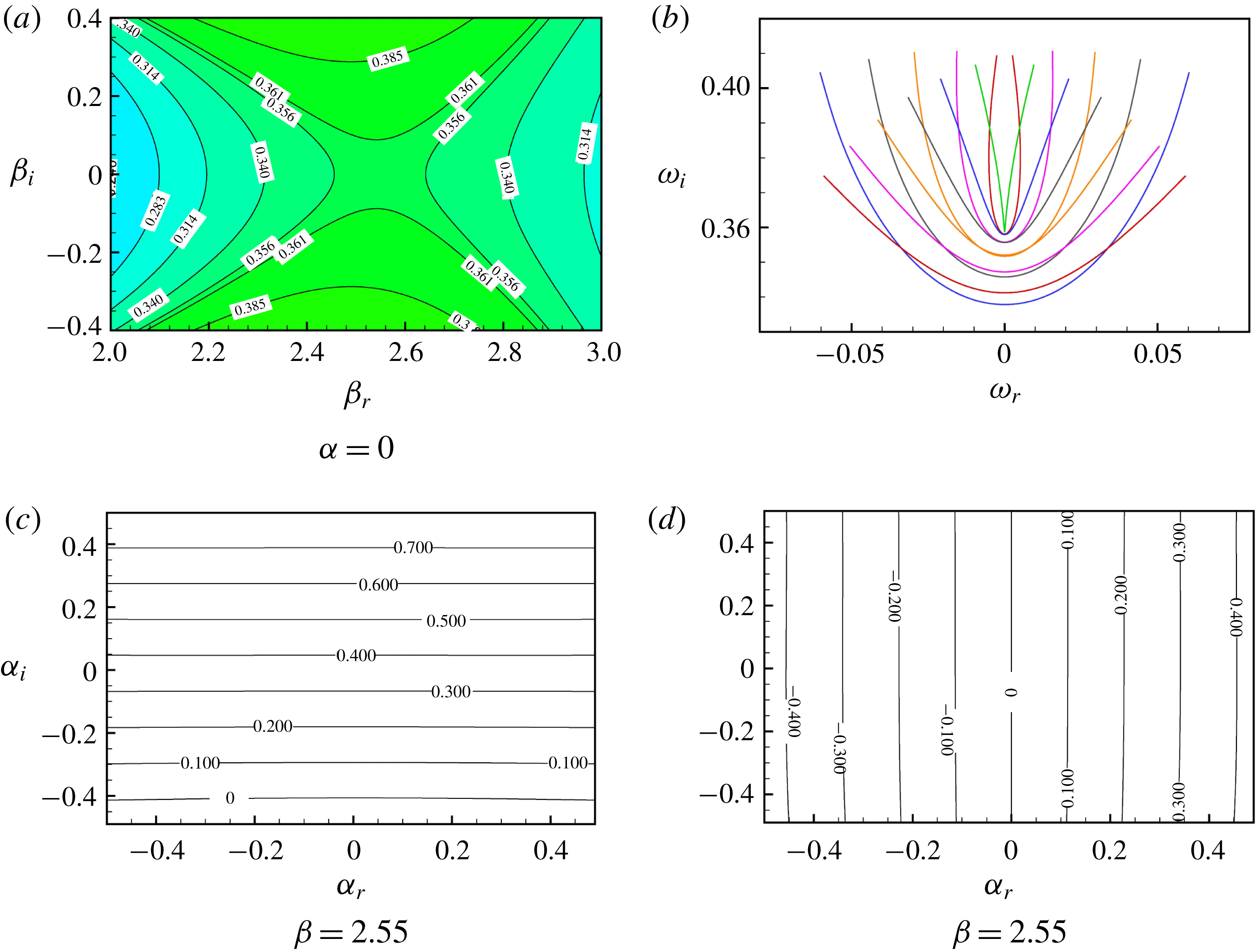
(the former represents a constant amplitude longitudinal roll while the latter admits amplitude variation). We performed a numerical search of the saddle point simultaneously in the streamwise and transverse wavenumber spaces. Figure 11(a) shows the saddle point located at
 $\unicode[STIX]{x1D6FD}=2.55$
in the
 $\unicode[STIX]{x1D6FD}$
plane with a positive absolute growth rate for longitudinal rolls
 $\unicode[STIX]{x1D6FC}=0$
at
 $T=200$
, indicating that the flow is absolutely unstable in the transverse direction. This is a trivial result as there is no cross-flow in the transverse direction. The corresponding cusp point can be identified in the
 $\unicode[STIX]{x1D714}$
plane, as shown in (b), confirming its validity. When we look into the contour of
 $\unicode[STIX]{x1D714}_{i}$
in the
 $\unicode[STIX]{x1D6FC}$
plane at
 $\unicode[STIX]{x1D6FD}=2.55$
(c), there is no saddle point at
 $\unicode[STIX]{x1D6FC}=0$
(or
 $\unicode[STIX]{x1D6FC}_{r}=0$
). In this case, the group velocity can be approximately calculated from (d) as 0.88 for
 ${\mathcal{U}}=1$
. Thus, these figures reveal no information about the growth rate at the ray
 $x/t=0$
regarding absolute/convective instability of LRs. At the critical condition
 $T=155.706$
, we see the same behaviour of LR, as shown in figure 12. We also checked the other values of
 $\unicode[STIX]{x1D6FD}$
for different
 $T$
and a similar result is observed.
(a) Longitudinal rolls. (b) The cusp point in the
 $\unicode[STIX]{x1D714}$
plane. (c) Contour of
 $\unicode[STIX]{x1D714}_{i}$
when
 $\unicode[STIX]{x1D6FD}=2.55$
in the
 $\unicode[STIX]{x1D6FC}$
plane. There is no saddle point. (d) Contour of
 $\unicode[STIX]{x1D714}_{r}$
when
 $\unicode[STIX]{x1D6FD}=2.55$
in the
 $\unicode[STIX]{x1D6FC}$
plane
 $T=200$
,
 $C=50$
,
 $M=50$
,
 $Fe=10^{4}$
.
(a) Longitudinal rolls at the critical condition (to be consistent with the one-mode Galerkin approximation). (b) The cusp point in the
 $\unicode[STIX]{x1D714}$
plane. (c) Contour of
 $\unicode[STIX]{x1D714}_{i}$
when
 $\unicode[STIX]{x1D6FD}=2.57$
in the
 $\unicode[STIX]{x1D6FC}$
plane. There is no saddle point. (d) Contour of
 $\unicode[STIX]{x1D714}_{r}$
when
 $\unicode[STIX]{x1D6FD}=2.57$
in the
 $\unicode[STIX]{x1D6FC}$
plane
 $T=155.706$
,
 $C=50$
,
 $M=50$
,
 $Fe=10^{4}$
.

In order to gain some insight into the absolute/convective instabilities of longitudinal rolls, we present in the following a one-mode Galerkin approximation of (2.19) and (2.20) following Carrière & Monkewitz (Reference Carrière and Monkewitz1999). The trial mode for the vertical velocity is
 $a_{1}v_{1}=a_{1}(1-y^{2})^{2}$
and for the electric potential
 $b_{1}\unicode[STIX]{x1D719}_{1}=b_{1}(y^{4}+4y^{3}-18y^{2}-4y+17)$
, where
 $a_{1},b_{1}$
are the coefficients. The slightly complex form of
 $\unicode[STIX]{x1D719}_{1}$
is due to its boundary conditions (2.21b
). Substituting these trial functions to the aforesaid equations, the one-mode Galerkin approximation leads to the following equations
 $$\begin{eqnarray}\displaystyle & & \displaystyle \left(U\text{i}\unicode[STIX]{x1D6FC}(k^{2}-D^{2})+U^{\prime \prime }\text{i}\unicode[STIX]{x1D6FC}+\frac{M^{2}}{T}(k^{4}-2k^{2}D^{2}+D^{4})\right)a_{1}v_{1}\nonumber\\ \displaystyle & & \displaystyle \quad +\,M^{2}[\unicode[STIX]{x1D6F7}^{\prime \prime \prime }k^{2}+\unicode[STIX]{x1D6F7}^{\prime }k^{2}(k^{2}-D^{2})]b_{1}\unicode[STIX]{x1D719}_{1}-\text{i}\unicode[STIX]{x1D714}(k^{2}-D^{2})a_{1}v_{1}=0,\end{eqnarray}$$
 $$\begin{eqnarray}\displaystyle & & \displaystyle -\unicode[STIX]{x1D6F7}^{\prime \prime \prime }a_{1}v_{1}+\left[\vphantom{\frac{1}{Fe}}\unicode[STIX]{x1D6F7}^{\prime \prime \prime }D+2\unicode[STIX]{x1D6F7}^{\prime \prime }(D^{2}-k^{2})+\unicode[STIX]{x1D6F7}^{\prime }(D^{3}-k^{2}D)+U\text{i}\unicode[STIX]{x1D6FC}(k^{2}-D^{2})\right.\nonumber\\ \displaystyle & & \displaystyle \quad +\left.\frac{1}{Fe}(k^{4}-2k^{2}D^{2}+D^{4})-\text{i}\unicode[STIX]{x1D714}(k^{2}-D^{2})\right]b_{1}\unicode[STIX]{x1D719}_{1}=0.\end{eqnarray}$$
 $v_{1}$
, the second equation with
 $\unicode[STIX]{x1D719}_{1}$
and integrating along the
 $y$
direction, we have
 $$\begin{eqnarray}\left(\begin{array}{@{}cc@{}}\text{i}\unicode[STIX]{x1D6FC}f_{1}+{\displaystyle \frac{M^{2}}{T}}f_{2}-\text{i}\unicode[STIX]{x1D714}f_{3} & M^{2}f_{4}\\ -f_{5} & f_{6}+\text{i}\unicode[STIX]{x1D6FC}f_{7}+{\displaystyle \frac{1}{Fe}}f_{8}-\text{i}\unicode[STIX]{x1D714}f_{9}\end{array}\right)\left(\begin{array}{@{}c@{}}a_{1}\\ b_{1}\end{array}\right)=0,\end{eqnarray}$$
where
 $f_{i}>0$
are some functions involving
 $k^{2}$
. Applying the solvability condition, we have
 $$\begin{eqnarray}\left(\unicode[STIX]{x1D6FC}f_{1}-\text{i}\frac{M^{2}}{T}f_{2}-\unicode[STIX]{x1D714}f_{3}\right)\left(-\text{i}f_{6}+\unicode[STIX]{x1D6FC}f_{7}-\text{i}\frac{1}{Fe}f_{8}-\unicode[STIX]{x1D714}f_{9}\right)-M^{2}f_{4}f_{5}=0.\end{eqnarray}$$
Following Carrière & Monkewitz (Reference Carrière and Monkewitz1999), we substitute
 $\unicode[STIX]{x1D714}=\unicode[STIX]{x1D714}^{\prime \prime }+\unicode[STIX]{x1D6FC}(x/t)$
(
 $\unicode[STIX]{x1D714}^{\prime \prime }$
is the temporal growth rate along the ray travelling at the group velocity
 $x/t$
and
 $y/t=0$
) and take the derivative of the above equation with respect to
 $\unicode[STIX]{x1D6FC}$
 $$\begin{eqnarray}\displaystyle & & \displaystyle \left(f_{1}-f_{3}\frac{x}{t}\right)\left(-\text{i}f_{6}+\unicode[STIX]{x1D6FC}f_{7}-\text{i}\frac{1}{Fe}f_{8}-\unicode[STIX]{x1D714}^{\prime \prime }f_{9}-\unicode[STIX]{x1D6FC}\frac{x}{t}f_{9}\right)\nonumber\\ \displaystyle & & \displaystyle \quad +\left(\unicode[STIX]{x1D6FC}f_{1}-\text{i}\frac{M^{2}}{T}f_{2}-\unicode[STIX]{x1D714}^{\prime \prime }f_{3}-\unicode[STIX]{x1D6FC}\frac{x}{t}f_{3}\right)\left(f_{7}-f_{9}\frac{x}{t}\right)=0.\end{eqnarray}$$
For longitudinal rolls
 $\unicode[STIX]{x1D6FC}=0$
, a special case is considered as
 $\unicode[STIX]{x1D714}^{\prime \prime }=0$
at the criticality
 $T=T_{c}$
and
 $\unicode[STIX]{x1D6FD}=\unicode[STIX]{x1D6FD}_{c}$
, so we have
 $$\begin{eqnarray}\left(f_{1}-f_{3}\frac{x}{t}\right)\left(f_{6}+\frac{1}{Fe}f_{8}\right)+\frac{M^{2}}{T_{c}}f_{2}\left(f_{7}-f_{9}\frac{x}{t}\right)=0,\end{eqnarray}$$
which is equivalent to
 $$\begin{eqnarray}\left.\frac{x}{t}\right|_{0}=\frac{f_{1}\left(f_{6}+{\displaystyle \frac{1}{Fe}}f_{8}\right)+{\displaystyle \frac{M^{2}}{T_{c}}}f_{2}f_{7}}{f_{3}\left(f_{6}+{\displaystyle \frac{1}{Fe}}f_{8}\right)+{\displaystyle \frac{M^{2}}{T_{c}}}f_{2}f_{9}}.\end{eqnarray}$$
In order to investigate the growth rate in the vicinity of
 $x/t|_{0}$
, we choose two rays
 $x/t_{\pm }$
on either side of
 $x/t|_{0}$
with
 $k^{2}=0$
and calculate the growth rates along these rays
 $$\begin{eqnarray}0<\frac{x}{t}_{-}=\left.\frac{f_{1}}{f_{3}}=\frac{1}{3}{\mathcal{U}}<\frac{x}{t}\right|_{0},\quad \text{Im}(\unicode[STIX]{x1D714}_{-}^{\prime \prime })=-\frac{M^{2}}{T_{c}}\frac{f_{2}}{f_{3}}<0,\end{eqnarray}$$
 $$\begin{eqnarray}\frac{x}{t}_{+}=\frac{f_{7}}{f_{9}}=\left.\frac{518}{153}{\mathcal{U}}>\frac{x}{t}\right|_{0},\quad \text{Im}(\unicode[STIX]{x1D714}_{+}^{\prime \prime })=-\frac{f_{6}+{\displaystyle \frac{1}{Fe}}f_{8}}{f_{9}}<0.\end{eqnarray}$$
 $x/t_{-}>0$
is chosen to be the same as that in Carrière & Monkewitz (Reference Carrière and Monkewitz1999), while
 $x/t_{+}$
is different than theirs partially because of the different trial function used for the imposed electric field. As the base profile of the electric field depends on the values of
 $C$
and
 $Fe$
, we have checked many values of these two parameters and the results show that both the imaginary parts of
 $\unicode[STIX]{x1D714}^{\prime \prime }$
are negative. It then can be deduced that at
 $x/t=0$
, the growth rate is negative, meaning that the flow cannot be absolutely unstable. Therefore, the LR is convectively unstable once there is a cross-flow.
With the convective nature of the longitudinal roll having been determined, we proceed to study the influence of the physical parameters on its instability. Figure 13 shows the neutral stability boundary in the
 $C$
–
 $T$
plane and the
 $Fe$
–
 $T$
plane. We see that the influence of the charge injection level
 $C$
and charge diffusion coefficient
 $Fe$
on the neutral stability boundary of longitudinal rolls is similar to their influence on transverse rolls as shown in figures 4(b) and 8(b), respectively.
The neutral stability boundary in the
 $C$
–
 $T$
plane (a) and
 $Fe$
–
 $T$
plane (b) for longitudinal rolls. The parameters in this figure are
 $M=50$
,
 $Fe=10^{4}$
.

The influence of the mobility ratio
 $M$
on the temporal growth rate
 $\unicode[STIX]{x1D714}_{i}$
is shown in figure 14(a). In the stable region where
 $\unicode[STIX]{x1D714}_{i}<0$
, the stability of longitudinal rolls is reinforced by increasing the mobility ratio. However, in the unstable region where
 $\unicode[STIX]{x1D714}_{i}>0$
, the effect of the mobility ratio becomes destabilising. It is noted that the mobility ratio does not influence the critical value of
 $T$
at which the transition from stability to instability occurs. The
 $M$
effect in LR is the same as in static EHD without a cross-flow.
(a) The influence of the mobility ratio
 $M$
on the growth rate
 $\unicode[STIX]{x1D714}_{i}$
of longitudinal rolls; (b) the influence of the base flow parameter
 ${\mathcal{U}}$
. The parameters in this figure are
 $C=50$
,
 $M=50$
,
 $Fe=10^{4}$
.

Finally, we consider the effect of the parameter
 ${\mathcal{U}}$
. As shown in figure 14(b), the dependence of the temporal growth rate
 $\unicode[STIX]{x1D714}_{i}$
on
 $T$
remains the same as
 ${\mathcal{U}}$
varies. That is,
 ${\mathcal{U}}$
has no influence on
 $\unicode[STIX]{x1D714}_{i}$
, which can be deduced as follows. When
 $\unicode[STIX]{x1D6FC}=0$
, it can be seen in (2.19) and (2.20) that the
 $U$
-related terms disappear because of their coupling to the streamwise spatial derivative. It is then the case that the magnitude of
 $U$
will not influence the instability characteristics of longitudinal rolls. In RBP flow, a similar conclusion has been reached in the study of longitudinal rolls.
3.4 Oblique rolls
In the following, we show briefly the results for oblique rolls (
 $\unicode[STIX]{x1D6FC}\neq 0$
,
 $\unicode[STIX]{x1D6FD}\neq 0$
). We first show in figure 15 that the growth rate of oblique rolls is always smaller than that of TR or LR in temporal (left column in the figure) and spatial stability analyses (right column) as the maximum growth rate is found either on
 $\unicode[STIX]{x1D6FC}$
or
 $\unicode[STIX]{x1D6FD}$
axis. In RBP flow, it has also been demonstrated by Pearlstein (Reference Pearlstein1985) that the most unstable mode should be either a transverse or a longitudinal roll.
(a,c,e) Typical
 $\unicode[STIX]{x1D714}_{i}$
-contours in the
 $\unicode[STIX]{x1D6FC}$
–
 $\unicode[STIX]{x1D6FD}$
plane for the temporal instability of oblique rolls; (b,d,f) typical
 $-\unicode[STIX]{x1D6FC}_{i}$
-contours in the
 $\unicode[STIX]{x1D6FC}_{r}$
–
 $\unicode[STIX]{x1D6FD}$
plane for the spatial instability of oblique rolls. The parameters in this figure are
 $C=50$
,
 $M=50$
,
 $Fe=10^{4}$
. Note that in (f) in the region where the transverse number
 $\unicode[STIX]{x1D6FD}$
is smaller than 2.34 the rolls become absolutely unstable and spatial analysis cannot be used.

The absolute growth rate
 $\unicode[STIX]{x1D714}_{0i}$
as a function of
 $\unicode[STIX]{x1D6FD}$
at saddle points (each data point corresponds to a saddle point). This figure aims to show at
 $\unicode[STIX]{x1D6FD}=0$
, the absolute growth rate is maximum.
 $T=230$
,
 ${\mathcal{U}}=1$
,
 $C=50$
,
 $M=50$
,
 $Fe=10^{4}$
.
 $\unicode[STIX]{x1D6FD}=0$
represents transverse rolls and
 $\unicode[STIX]{x1D6FD}\neq 0$
oblique rolls.

To study the absolute and convective instability of oblique rolls, according to the method described in § 2.4, we need to find the saddle points in both the
 $\unicode[STIX]{x1D6FC}$
and
 $\unicode[STIX]{x1D6FD}$
planes, satisfying the pinching condition. Fortunately, due to the symmetry of the problem in the transverse direction, the maximum growth rate is found at
 $\unicode[STIX]{x1D6FD}=0$
. This is numerically examined in figure 16, in which we see that the absolute growth rate at the saddle point decreases when
 $\unicode[STIX]{x1D6FD}$
increases. This indicates that the absolute growth rate for the transverse rolls is larger than that of oblique rolls. Such a numerical check only tackles one real line in the complex
 $\unicode[STIX]{x1D6FD}$
plane. We also conducted a numerical search for the saddle points simultaneously in the complex
 $\unicode[STIX]{x1D6FC}$
and
 $\unicode[STIX]{x1D6FD}$
spaces and found that, in the
 $\unicode[STIX]{x1D6FD}$
plane, the saddle point is always located at
 $\unicode[STIX]{x1D6FD}=0$
, confirming the transverse symmetry and implying that if the flow is absolutely unstable, TR will appear rather than an oblique roll. Therefore, we deduce that the oblique rolls are not significant in the CI–AI transition of EHD-Poiseuille flow and are not expected to be observed in the experiments. Oblique rolls were not present in the numerical simulations of RBP by Martinand, Carrière & Monkewitz (Reference Martinand, Carrière and Monkewitz2006). In Carrière & Monkewitz (Reference Carrière and Monkewitz1999), they commented that the boundary of absolute instability in RBP coincides with the absolute instability boundary for transverse rolls due to transverse symmetry.
4 Concluding remarks
In this work, we have applied spatio-temporal linear stability analysis to EHD-Poiseuille flow in the SCL regime in order to investigate its absolute and convective instabilities, supplementing the previous studies on the linear stability analysis of this flow (Castellanos & Agrait Reference Castellanos and Agrait1992; Lara et al.
Reference Lara, Castellanos and Pontiga1997; Zhang et al.
Reference Zhang, Martinelli, Wu, Schmid and Quadrio2015). We considered three different roll structures. Physical parameters such as
 $T$
,
 $M$
,
 $C$
,
 $Fe$
,
 ${\mathcal{U}}$
are probed with an aim of clarifying their effects on the absolute–convective instability transition. These results are important to understand in general the effect of an electric field applied in a cross-flow, for example, in the case of electrostatic precipitators, flow control or heat transfer enhancement using EHD.
The effects of non-dimensional parameters are briefly summarised here. For TR, we found that increasing
 $T$
(Coulomb force to viscous force) or electric voltage
 $V_{0}$
will make the flow transition from being convectively unstable to absolutely unstable. Since the flow we considered is in the SCL regime, the effect of the ion injection level
 $C$
on the CI–AI transition is not significant except at small
 $C$
. Small mobility ratio
 $M$
is associated with a saddle point shift phenomenon and subsequently, the critical
 $T$
in this condition for CI–AI transition is boosted to a much higher value. Physically this is because that small
 $M$
tends to make the hydrodynamical field decouple from the electric effect, rendering it more stringent to becoming absolutely unstable (due to the convective nature of Poiseuille flow). Stronger charge diffusion will facilitate flow instability, towards absolute instability. Understanding its instability mechanism is beyond the current work and is currently under investigation. The critical
 $T$
increases with increasing magnitude of the cross-flow.
This paper is written with an objective to serve as a source of comparison and theoretical guidance for future laboratory measurements of the absolute/convective instabilities in a real dielectric fluid subject to unipolar injection. Our findings that the experimentalists may find useful and interesting and are subject to verification include that (i) near CI–AI transition, the absolute growth rate increases quadratically as a function of the applied voltage (which is the most straightforward means to change in experiments), that (ii) when
 $T$
is large and
 $M$
relatively small, localised flow structures appear close to the injector at the saddle condition and that (iii) when the amplitude of the cross-flow is small, TR is more likely to appear in the experiments than LR and the TR can exhibit absolute instability in EHD-Poiseuille flow. When
 ${\mathcal{U}}$
is large, LR has a higher growth rate than TR and is preferred at this condition. Besides, our results also show that the LR is convectively unstable and for oblique rolls, the growth rate is always smaller than that of TR/LR.
This work focuses on the linear nature of the absolute and convective instabilities in EHD-Poiseuille flow. When the disturbance grows to some extent, a nonlinear analysis is employed for the subsequent development of the disturbance, for which a direct numerical method is usually employed. A nonlinear analysis (Chomaz Reference Chomaz1992) is suggested to be undertaken in the future as it will reveal more thoroughly the roll transition mechanism in EHD-Poiseuille flow. Besides, the absolute/convective instability in other EHD flows subject to a cross-flow, which are more directly related to the practical problems, such as wire-two-plate geometry in McCluskey & Atten (Reference McCluskey and Atten1984) and ESP (Leonard et al. Reference Leonard, Mitchner and Self1983; Atten et al. Reference Atten, McCluskey and Lahjomri1987), can be studied similarly, as we have suggested above.
Acknowledgements
F.L. and B.W. acknowledge the financial support by the National Natural Science Foundation of China (Project nos. 11772328, 11621202 and 11502137). M.Z. acknowledges the Start-up grant from the Ministry of Education, Singapore (MOE WBS no. R-265-000-619-133). We thank all the referees for their constructive suggestions.
Appendix A. Method to find saddle points
A double iteration method is used to calculate saddle points in the three-dimensional case. The procedure is as follows: first, give four initial values of
 $\unicode[STIX]{x1D6FD}$
, i.e.
 $\unicode[STIX]{x1D6FD}_{1}$
,
 $\unicode[STIX]{x1D6FD}_{2}$
,
 $\unicode[STIX]{x1D6FD}_{3}$
and
 $\unicode[STIX]{x1D6FD}_{4}$
, near a saddle point in the complex
 $\unicode[STIX]{x1D6FD}$
-plane; for each initial value of
 $\unicode[STIX]{x1D6FD}$
, i.e.
 $\unicode[STIX]{x1D6FD}_{j}$
, calculate the corresponding saddle point in the complex
 $\unicode[STIX]{x1D6FC}$
-plane using the iteration method employed in Yin & Sun (Reference Yin and Sun2003). That is, given four values of
 $\unicode[STIX]{x1D6FC}$
, i.e.
 $\unicode[STIX]{x1D6FC}_{1}$
,
 $\unicode[STIX]{x1D6FC}_{2}$
,
 $\unicode[STIX]{x1D6FC}_{3}$
and
 $\unicode[STIX]{x1D6FC}_{4}$
, near the saddle point, calculate the corresponding values of
 $\unicode[STIX]{x1D714}$
, i.e.
 $\unicode[STIX]{x1D714}_{1}$
,
 $\unicode[STIX]{x1D714}_{2}$
,
 $\unicode[STIX]{x1D714}_{3}$
and
 $\unicode[STIX]{x1D714}_{4}$
, and then construct the following interpolation function
 $$\begin{eqnarray}\unicode[STIX]{x1D714}(\unicode[STIX]{x1D6FC}_{i})=\frac{a}{3}(\unicode[STIX]{x1D6FC}_{i}-\unicode[STIX]{x1D6FC}_{4})^{3}+\frac{b}{2}(\unicode[STIX]{x1D6FC}_{i}-\unicode[STIX]{x1D6FC}_{4})^{2}+c(\unicode[STIX]{x1D6FC}_{i}-\unicode[STIX]{x1D6FC}_{4})+d,\end{eqnarray}$$
where the subscript
 $i=1,2,3,4$
. The coefficients
 $a$
,
 $b$
,
 $c$
and
 $d$
are readily solved by substituting the four couples of
 $\unicode[STIX]{x1D6FC}$
and
 $\unicode[STIX]{x1D714}$
into (A 1). Naturally, the value of
 $\unicode[STIX]{x1D6FC}$
at the saddle point is supposed to be the solution of the following equation
 $$\begin{eqnarray}\frac{\text{d}\unicode[STIX]{x1D714}}{\text{d}\unicode[STIX]{x1D6FC}}=a(\unicode[STIX]{x1D6FC}-\unicode[STIX]{x1D6FC}_{4})^{2}+b(\unicode[STIX]{x1D6FC}-\unicode[STIX]{x1D6FC}_{4})+c=0.\end{eqnarray}$$
Solving (A 2), we obtain
 $\unicode[STIX]{x1D6FC}_{5}$
. Then we use
 $\unicode[STIX]{x1D6FC}_{2}$
,
 $\unicode[STIX]{x1D6FC}_{3}$
,
 $\unicode[STIX]{x1D6FC}_{4}$
and
 $\unicode[STIX]{x1D6FC}_{5}$
as four known values in the interpolation function (A 1), and calculate the saddle point again in (A 2). The iteration is terminated when a convergence request is reached (e.g. the relative error of
 $\unicode[STIX]{x1D6FC}$
or
 $\unicode[STIX]{x1D714}$
is not larger than 0.005). Thus we obtain
 $\unicode[STIX]{x1D6FC}_{0j}$
and
 $\unicode[STIX]{x1D714}_{0j}$
at the saddle point in the complex
 $\unicode[STIX]{x1D6FC}$
-plane that correspond to
 $\unicode[STIX]{x1D6FD}_{j}$
; then, in complex
 $\unicode[STIX]{x1D6FD}$
-plane, four couples of
 $\unicode[STIX]{x1D6FD}_{j}$
and
 $\unicode[STIX]{x1D714}_{0j}$
are used to build an interpolation function similar to (A 1)
 $$\begin{eqnarray}\unicode[STIX]{x1D714}(\unicode[STIX]{x1D6FD}_{j})=\frac{a}{3}(\unicode[STIX]{x1D6FD}_{j}-\unicode[STIX]{x1D6FD}_{4})^{3}+\frac{b}{2}(\unicode[STIX]{x1D6FD}_{j}-\unicode[STIX]{x1D6FD}_{4})^{2}+c(\unicode[STIX]{x1D6FD}_{j}-\unicode[STIX]{x1D6FD}_{4})+d,\end{eqnarray}$$
where
 $j=1,2,3,4$
, and the saddle point in the complex
 $\unicode[STIX]{x1D6FD}$
-plane is determined by
 $$\begin{eqnarray}\frac{\text{d}\unicode[STIX]{x1D714}}{\text{d}\unicode[STIX]{x1D6FD}}=a(\unicode[STIX]{x1D6FD}-\unicode[STIX]{x1D6FD}_{4})^{2}+b(\unicode[STIX]{x1D6FD}-\unicode[STIX]{x1D6FD}_{4})+c=0.\end{eqnarray}$$
Solving (A 4), we obtain
 $\unicode[STIX]{x1D6FD}_{5}$
; for this
 $\unicode[STIX]{x1D6FD}_{5}$
, Yin & Sun’s iteration method is used again to calculate the corresponding
 $\unicode[STIX]{x1D6FC}_{05}$
and
 $\unicode[STIX]{x1D714}_{05}$
at the saddle point in the complex
 $\unicode[STIX]{x1D6FC}$
-plane; then, replacing
 $\unicode[STIX]{x1D6FD}_{1}$
,
 $\unicode[STIX]{x1D714}_{01}$
by
 $\unicode[STIX]{x1D6FD}_{5}$
,
 $\unicode[STIX]{x1D714}_{05}$
in (A 3), we calculate
 $\unicode[STIX]{x1D6FD}_{6}\ldots$
until it converges. Finally we get the values of
 $\unicode[STIX]{x1D6FC}_{0}$
,
 $\unicode[STIX]{x1D6FD}_{0}$
and
 $\unicode[STIX]{x1D714}_{0}$
at the saddle points in both the complex
 $\unicode[STIX]{x1D6FC}$
- and complex
 $\unicode[STIX]{x1D6FD}$
-planes. For an overview of the numerical methods of locating saddle points in wavenumber space using the viscous dispersion relation, one is referred to Suslov (Reference Suslov2006).



