1 Introduction
Automatically learning models from training examples is a very attractive way to solve many complex tasks in natural language processing (NLP). Learning algorithms generally discover important information which could be otherwise only manually encoded in rule-based systems. In recent work, they have shown a good level of accuracy for most natural language tasks: part-of-speech tagging, named entity recognition, word-sense disambiguation, and semantic role labeling.
Regarding the Recognizing Textual Entailment (RTE) challenges (Bar-Haim et al. Reference Bar-Haim, Dagan, Dolan, Ferro, Giampiccolo, Magnini and Szpektor2006; Dagan, Glickman and Magnini Reference Dagan, Glickman, Magnini, Quiñonero-Candela, Dagan, Magnini and d'Alché-Buc2006; Giampiccolo et al. Reference Giampiccolo, Magnini, Dagan and Dolan2007), supervised machine learning (ML) models have proved to be particularly successful in solving the task, despite the fact that their application to RTE is difficult, as textual entailment is an extremely complex natural language phenomenon. Generally, NLP tasks require a classifier to assign the correct label to a target text fragment, looking at its context. For example, in semantic role labeling (e.g., see Gildea and Jurafsky Reference Gildea and Jurafsky2002; Carreras and Màrquez Reference Carreras and Màrquez2005), the goal is to assign the correct role to a relevant text fragment with respect to a set of possible roles (e.g., Agent, Patient). For this purpose, a model of the context of the fragment, at a specific level of linguistic representation (e.g., bag-of-word models or syntactic interpretations) is typically used. In contrast, textual entailment recognition requires processing two different texts between which complex semantic/syntactic relations hold, and the goal is to classify such relations as true or false entailment. Typical bag-of-word models are not useful to capture the knowledge needed by the learning algorithms.
In this paper we propose a solution to the above problem, by introducing a new type of feature space, the pair feature space, which allows learning algorithms to exploit the relations between a text (T) and a hypothesis (H).
To explain the novelty of our approach, we first analyze what type of knowledge a general RTE model needs for solving the task and explain how learning algorithms typically learn it (Section 2). In Section 2.1 we introduce the notion of ground rewrite rules (rules without variables) and first-order rewrite rules (rules with variables) and describe how they are used by rule-based systems. In Section 2.2 we show that ML algorithms can learn some of these rules, using different types of feature spaces. Accordingly, we propose a classification of feature spaces in four types: the similarity, the entailment trigger, the content, and the pair content feature spaces. We will demonstrate that none of these spaces offers the possibility to learn first-order rewrite rules, which are those that more effectively model the relations between T and H.
In Section 3, we will propose our solution to learn first-order rewrite rules or first-order rewrite derivations via the pair feature space. This space is based on the notion of placeholders, which explicitly model relations between T and hypothesis H. Pairs enriched with placeholders help ML algorithms to extract and exploit first-order rewrite rules from training examples and to apply them to classify new ones. In Section 4 we describe an extension of the model, integrating shallow semantic information. Finally, in Section 5, we experiment with our models and show that the pair feature space helps in exploiting first-order rewriting rules implicitly defined in training examples.
2 RTE models and supervised ML
Many approaches to RTE rely on rewrite rules to detect entailment between text and hypothesis. Such rules are built at different linguistic levels: lexical, syntactic, and semantic. We here aim at drawing a second important distinction, between ground and first-order rewrite rules. The former are rules that do not allow the use of variables, while the latter do. A ground rewrite rule can be applied to detect implications in a very small set of cases, e.g., ‘The sun emits UVA rays’ → ‘Tanning can expose to health risks’. On the contrary, a first-order rewrite rule can be applied to many entailment examples, e.g., ‘X killed Y’ → ‘Y died’.
These rules thus offer an appealing level of generalization that can be exploited while either hand-crafting or automatically learning rules for RTE. Modeling feature spaces that allow ML algorithms to discover first-order rewrite rules is not easy, as we show hereafter.
In the remainder of this section, we briefly outline typical rule-based approaches for RTE (Section 2.1) and classify existing feature spaces according to the kind of rules they encode (Section 2.2). We show that existing feature spaces do not fully exploit first-order rewrite rules encoded in training examples, as this needs the introduction of variables in the feature space. This last point is the main contribution of our paper, and it will be described in Section 3.
2.1 Rewrite rules and rule-based systems
Ground and first-order rewrite rules are largely used to encode knowledge in RTE systems, operating at different levels of interpretation: lexical, syntactic, or semantic.
Ground rewrite rules transform a text into a new text. The object of the transformation appears in the rules as a ground atom. Thus, for any transformation a different rule is needed. Most RTE systems apply ground rules at the lexical level (e.g., de Salvo Braz et al. Reference de Salvo Braz, Girju, Punyakanok, Roth and Sammons2005a) transforming a word into a new entailed word (e.g., chairman → president) or a sequence of words into a new sequence. At the syntactic level, they typically transform syntactic structures (e.g., parse-trees portions) into new ones (Kouylekov and Magnini Reference Kouylekov and Magnini2005). At the semantic level they can transform predicative structures. Ground rewrite rules suffer from the limitation that they can encode only non-generalized knowledge. For example, the rule ‘Oswald killed JFK’ → ‘JFK died’ models a commonly agreed non-generalized piece of knowledge. Yet, it would be more effective to rely on the generalized knowledge that if ‘someone kills someone else’, then ‘someone else dies’.
First-order rewrite rules solve the previous problem, by introducing variables. In the above example, the generalized knowledge would be captured by the rule ‘X killed Y’ → ‘Y died’, where the Y on one side of the rule is unified with that on the other side of the rule. Another example is the rule modeling the predicative reading of an apposition:

First-order rewrite rules are mostly exploited at the lexical level (e.g., Marsi, Krahmer and Bosma Reference Marsi, Krahmer and Bosma2007) or at the syntactic level (e.g., de Salvo Braz et al. Reference de Salvo Braz, Girju, Punyakanok, Roth and Sammons2005a) to represent structured knowledge of manually built (e.g., FrameNet; Baker, Fillmore and Lowe Reference Baker, Fillmore and Lowe1998) or automatically acquired (e.g., Lin and Pantel Reference Lin and Pantel2001) lexical databases. These rules thus offer an appealing level of generalization to encode knowledge for RTE.
The design of rule-based RTE systems encoding ground or first-order rules is particularly expensive, for two main reasons: (i) The complete coverage of the entailment phenomenon may require large sets of specific rules; (ii) rewrite rules are written at a given language interpretation level: good rules applied at wrong levels of sentences interpretation can lead to wrong decisions.
Typical approaches address these problems using a weighting schema. A weight is assigned to each rule when rules are applied to transform the text into the hypothesis. These rule weights are used to compute a score for the overall transformation, representing the validity of the whole process. A manually derived threshold is then applied to the score to determine the polarity of the entailment.
2.2 ML models for RTE
ML algorithms can alleviate the rule design process described in the previous section in two ways: (1) determining the weight of known rules and the threshold of the overall process; (2) discovering previously unknown rules. The major issue in using ML approaches is the definition of a representation of text and hypothesis which allows for an effective learning of the entailment recognition rules. In other words, we need to define features able to capture the knowledge enclosed in the typical rewrite rules used by rule-based systems.
By carefully examining previous work, we note that most ML-based systems for RTE perform one of the following functions: (i) apply similarity measures between text (T) and hypothesis (H) (Corley and mihalcea Reference Corley and Mihalcea2005; Newman et al. Reference Newman, Stokes, Dunnion, Carthy, Candela, Dagan, Magnini and Buc2005; Hickl et al. Reference Hickl, Williams, Bensley Roberts, Rink, Shi, Magnini and Dagan2006); (ii) extract content from the T and H pairs (Zanzotto and Moschitti Reference Zanzotto and Moschitti2006); (iii) define rules that strongly suggest the implications (triggers) (de Marneffe et al. Reference de Marneffe, MacCartney, Grenager, Cer, Rafferty, Manning, Magnini and Dagan2006; MacCartney et al. Reference MacCartney, Grenager, de Marneffe, Cer and Manning2006); or (iv) extract more general features, e.g., word or syntactic construction pairs, that describe all the possible rewrite rules encoded in pairs.
According to the above classification, we define four different types of feature spaces: similarity space, content, entailment trigger, and paired-content feature spaces.
2.2.1 Similarity feature space
In this space, the basic hypothesis is that if two sentences are similar, then they are likely to be in entailment. Similarity between T and H can be captured in different ways and at different levels (lexical, syntactic, and semantic) (e.g., Inkpen, Kipp and Nastase Reference Inkpen, Kipp., Nastase, Magnini and Dagan2006). Each feature encodes a different similarity between T and H. Most RTE systems use a feature space at the lexical level (hereafter called lex space). For example, a feature could count the percentage of content words of H that are equal to words in T or that are semantically related to words in T (e.g., Corley and Mihalcea Reference Corley and Mihalcea2005). Another feature could model the length of the longest common subsequence (LCS) between T and H (e.g., Newman et al. Reference Newman, Stokes, Dunnion, Carthy, Candela, Dagan, Magnini and Buc2005; Hickl et al. Reference Hickl, Williams, Bensley Roberts, Rink, Shi, Magnini and Dagan2006): the longer the LCS, the more likely it is that the meaning of H is included in the meaning of T. At the syntactic level, a feature could represent the percentage of dependencies that H has in common with T (as in Haghighi, Ng and Manning Reference Haghighi, Ng and Manning2005; Pazienza, Pennacchiotti and Zanzotto Reference Pazienza, Pennacchiotti and Zanzotto2005) or the longest common subtree between H and T (Katrenko and Adriaans Reference Katrenko, Adriaans, Magnini and Dagan2006). At the semantic level, a feature could be the percentage of semantic relations of H shared with T.
In terms of rewriting rules, these feature spaces generally exploit lexical ground rules such as those that connect semantically related words and, basically, only one first-order rule, i.e., the identity rule that transforms X → X.
Limits. The similarity feature space produces effective entailment classifiers but is not sufficient to model RTE: the fact that two texts are similar does not always imply that they are in entailment. For example, at the lexical level, if fragments differ only by the presence of a negation, they are not in entailment, even if their lexical similarity is very high. Similarly, at the syntactic level, two very dissimilar fragments can be still in entailment when a syntactic alternation takes place (e.g., active/passive, paraphrases) or when downward and upward monotonicity is involved, as in the following example:
In the example, T 2 entails H 2 but it does not entail H 3: in a lexical similarity feature space, these two examples would have the same vector.
2.2.2 The content feature space
Similarity feature spaces constrain the description of entailment phenomena to simple similarity. These spaces are then unable to describe properties which are contained in T or H. The content feature space (hereafter cont) aims at solving this drawback by modeling the content of T and H. This can include lexical, syntactic, or semantic features of the two fragments. Specifically, T and H are separately represented by two distinct and independent sets of features. The major advantage of this space is that rewrite rules can be automatically learned from a training set and successively applied to determine the polarity of a test pair.
For example, consider the space of syntactic subtrees

. The features are the set of all subtrees h ∈
of H and the set of all subtrees t ∈
of T. Such space is useful for solving complex cases that cannot be processed in other ones, like the examples (T 2, H 2) and (T 3, H 3) reported in Section 2.2.1. Let us assume that the T and the H of the two examples are represented as syntactic trees, as follows:
While in the similarity feature space (T 4, H 4) and (T 5, H 5) are identical, here they are represented by two different feature vectors, since H 4 and H 5 have different syntactic structures (‘all solid insurance companies’ is different from ‘all solid companies’ and ‘dividends’ is different from ‘cash dividends’). If we then want to classify the example
T and H structures are globally more similar (i.e., in terms of number of common tree fragments) to (T 4, H 4) than to (T 5, H 5).
These feature spaces model independently the right-hand side and the left-hand side of ground rewrite rules. ML algorithms can learn both new ground rules or ground rule fragments and their associated weights.
Limits. Since the feature spaces of T and H are independent, rules that exploit the relations between some properties of T and some properties of H cannot be derived; i.e., most of the properties should be matched to trigger the selection of the best representative training example. For example, the pair ‘Oswald killed JFK’ → ‘JFK died’ cannot be used to determine the polarity of ‘Oswald killed JFK by shooting him several gun bullets’, ‘JFK died’, since there is too much difference in terms of syntactic/semantic content in the fragments.
2.2.3 The entailment trigger feature space
A limit of the previous space is that it does not extract joint features from a (T, H) pair. The entailment trigger feature space (hereafter trig) overcomes such a limitation (along with those of the similarity feature space) by modeling complex relations between T and H. The underlying hypothesis is that entailment holds (or does not) if specific rewrite rules (i.e., triggers) stand between T and H. Triggers can be either positive or negative, if they respectively suggest entailment or don't. Each feature of the space represents a specific trigger; i.e., its value can be 0 or 1 whether the trigger is present or not in the given (T, H) pair. This approach has been successfully explored in de Marneffe et al. (Reference de Marneffe, MacCartney, Grenager, Cer, Rafferty, Manning, Magnini and Dagan2006) and MacCartney et al. (Reference MacCartney, Grenager, de Marneffe, Cer and Manning2006) by means of the following triggers:
• Polarity features. Presence/absence of negative polarity contexts (not, no or few, without), as in ‘Oil price surged’ ↛ ‘Oil prices didn't grow’.
• Antonym features. Presence/absence of antonymous words in T and H. These features capture cases such as ‘Oil price is surging’ ↛ ‘Oil prices is falling down’.
• Adjunct features. Dropping/addition of syntactic adjunct when moving from T to H, as in ‘all solid companies pay cash dividends’ → ‘all solid companies pay dividends’.
• Passive features. Presence/absence of a transformation from active to passive, moving from T to H or vice versa.
These feature spaces model specific ground or first-order rewrite rules. ML algorithms learn the weights of the rules and the final threshold to apply.
Limits. The trigger feature space has two limitations: (1) rules should be all known and hand-coded in advance; (2) rule composition cannot be explicitly stated, since features are flat and independent entities—i.e., the feature space can only model that two triggers are true, but cannot directly express the fact that one trigger must be applied before another in order to predict a true or false entailment.
2.2.4 The paired-content feature space
Similarly to the cont space, the underlying hypothesis of the paired-content feature space (hereafter p_cont) is that evidence of entailment (rules and distances) should emerge directly from the explicit content of T and H, instead of being manually coded a priori. Yet, here T and H are not represented by two independent feature sets. Instead, in this space a (T,H) pair is represented by pairs of features from T and H so that the learner can acquire ground rewrite rules (i.e., relational properties between the two texts). The paired content can be either a lexical, a syntactic, or a semantic representation of the two fragments.
As an example, consider the space of syntactic subtrees
introduced in the previous section; p_cont is the set of subtree pairs 〈t, h〉 ∈
×
, where T and H are two subtrees of T and H respectively. Some meaningful pairs may suggest the syntactic properties, e.g., triggers, which T and H must have to be in an entailment relation. This allows to overcome the limits of the cont space, since only the properties of H and T that model a useful trigger are matched. For example, suppose that H 5 contains an irrelevant part (e.g., ‘All solid companies pay cash dividends, but other companies do not’). In cont, H 5 would now result more similar to H 4 than to H 5 because it shares a higher percentage of subtrees with H 4. The entailment prediction of the system would then be incorrect. Instead in the p_cont space, the model for (T 4, H 4) contains the feature (fragment pair)
which does not depend on any additional content. This feature is also present in the feature space of (T 6, H 6), but not in (T 5, H 5), suggesting that (T 6, H 6) is correctly more similar to (T 4, H 4). In this case, the above feature can be then considered as a ground rewrite rule.
The p_cont space models ground rewrite rules. According to the learning examples, ML algorithms select interesting rules, learn the associated weights, and determine the final threshold to apply.
Limits. The paired-content feature space allows learning only ground rewrite rules. To learn first-order rewrite rules we need to introduce variables in the text representation, i.e., by making explicit the relations between elements in the texts and elements in the hypotheses. As it is, p_cont can induce incomplete or erroneous rewrite rules. For example, consider the following entailment pair:
When p_cont is built on syntactic structures, it contains (among the others) the structure pair
The problem is that this trigger is contained in both the following entailment cases:
where T 10 entails H 10 whereas T 11 does not entail H 11.
This suggests that ground feature pairs (rules) are not powerful enough to generalize different examples. In contrast, with the use of variables, first-order rewrite rules solve the problem; e.g., the rule
applies (belong) to only the first example.
3 Learning first-order rules in a syntactic paired-content feature space
In the previous section we presented four different feature spaces along with their limits and properties. It is interesting to notice that in terms of expressiveness, the similarity and the content feature spaces (lex and cont) are orthogonal and can be both included in the trigger feature space. With the latter, we mean a space in which features/rules are manually selected at the underlying representation layer, e.g., syntactic parse trees or shallow semantic structures, of (T, H).
Moreover, the p_cont space learns (i.e., generates) ground rules in terms of feature pairs. In order to allow it to model first-order rules, we need to introduce variables in the representation layer. To do so, we use kernel methods and support vector machines (SVMs). In this framework, we define a space and the related kernel function which allows to extract and exploit first-order rewrite rules from annotated examples.
The remainder of this section is organized as follows: first, we introduce the idea of learning first-order rewrite rules (Section 3.1); second, we describe how a pair feature space including variables can be obtain from examples (Section 3.2); third, we discuss how to obtain these feature spaces by using kernel functions (Section 3.3).
3.1 Learning first-order rewrite rules
Our proposal for learning first-order rewrite rules stems from the observation that the trig and the p_cont spaces are strictly related. Indeed, if we restrict trig to model only ground rewrite rules, then it represents a subset of p_cont. For example, the trig
is included in the syntactic content feature space (defined in Section 2.2.4), as it models the corresponding feature:
As shown in the previous sections, typical handcraft rules contain variables. Thus, to obtain the same expressiveness of the entailment trigger feature space with the paired-content feature space, we need to find a way to include variables as content. This allows ML algorithms to learn first-order rules implicitly described in training examples. In such space a pair 〈T, H〉 is represented as follows:

where  (T) and (H) are the sets of features derivable from a structured representation of T and H. If in (T) and (H) variables are somehow defined, each pair 〈ft, fh〉 represents in general a first-order derivation described in the (T, H) example.
3.2 Three syntactic pair feature spaces
We have shown that the p_cont space is the most promising to encode effective knowledge for Textual Entailment (TE). However, as different linguistic levels can be adopted to represent T and H (lexical, syntactic, semantic), we here need to choose the most relevant, in order to better focus our study.
For this purpose, we note that a large part of the entailment cases depend on the syntactic structure of T and H (Vanderwende and Dolan Reference Vanderwende, Dolan, Candela, Dagan, Magnini and Buc2006). More specifically, grammar rules are most useful, as they can reduce data sparseness by generalizing word sequences expressed with the same syntax. In our case, the set P in (1) can be generalized by using syntactic derivations (i.e., the sequence of production rules) that in turn generate word sequences in the training examples.
We here present three feature spaces (which are subsets of the more general paired-content feature space) that capture the above intuition: a ground syntactic rule feature space and two first-order syntactic rule feature spaces. The first space is used as the basis space to define the other two.
3.2.1 A ground syntactic rule feature space
The syntactic paired-content feature space (synt) models entailment pairs using the set of tree fragment pairs (for an example of different fragment types see Moschitti Reference Moschitti2006a), similar to the syntactic content feature space. A pair 〈T, H〉 is represented as follows:

where
(⋅) indicates the set of fragments of the sentence parse tree given as argument. For instance, given T 4 and H 4 of the example in Section 2.2.4, we have the following relational description:
This clearly models ground rewrite derivations between T and H; e.g., the pair 〈[VP [VBP bought] [NP]], [VP [VBP own] [NP]]〉 models the ground rewrite rule [VP [VBP bought] [NP]] → [VP [VBP own] [NP]].
3.2.2 Two first-order syntactic rule feature spaces
In this section, we have proposed two first-order syntactic rule feature spaces: the syntactic pair feature space with placeholders in the preterminal nodes (plac_basic) and the syntactic pair feature space with propagated placeholders (plac_all).
plac_basic. This space introduces variables in the pairs, by applying an anchoring algorithm, which works as follows.
Before deriving the tree fragments we augment the syntactic tree with placeholders. A placeholder is a label assigned to an anchor. Anchors are nodes from τt and τh dominating the same (or similar) information. As many other approaches (e.g., Corley and Mihalcea Reference Corley and Mihalcea2005; Glickman, Dagan and Koppel Reference Glickman, Dagan and Koppel2005), our anchoring model is based on a similarity measure between words simw(wt, wh). Specifically, we anchor the content words (verbs, nouns, adjectives, and adverbs) in the hypothesis WH to words in the text WT, by using a two-step greedy algorithm.
In the first step, each word wh in WH is connected to all words wt in WT that have the maximum similarity simw(wt, wh) with it. (More than one wt can have the maximum similarity with wh.) As result, we have a set of anchors A ⊂ WT × WH; simw(wt, wh) is computed by means of three techniques:
(1) Two words are maximally similar if they have the same surface form, wt = wh.
(2) Otherwise, WordNet (Miller Reference Miller1995) similarities (as in Corley and Mihalcea Reference Corley and Mihalcea2005) and different relation between words such as verb entailment and derivational morphology are applied.
(3) The edit distance measure is finally used to capture the similarity between words that are missed by the previous analysis (for misspelling errors or for the lack of derivational forms in WordNet).
In the second step, we select the final anchor set A′ ⊆ A, such that ∀wt (or wh) ∃!〈wt, wh〉 ∈ A′. The selection is based on a simple greedy algorithm. Given two pairs 〈wt, wh〉 and 〈w′t, wh〉 to be selected and a pair 〈st, sh〉 already selected, the algorithm considers word proximity (in terms of number of words) between wt and st and between wt′ and st, and it chooses the nearest word.
Once the set A′ is found, anchors are encoded in the syntactic trees with placeholders. Placeholders are put on the preterminal nodes of the anchored words. For example, the pair (T 10, H 10) can be augmented with placeholders as follows:
We then obtain the following richer representation based on fragment pairs:
Placeholders (or variables)

and

specify that the NNPs labeled by the same variables dominate similar or identical words. The first pair of the set P τp describes a first-order rewriting derivation between T and H. Therefore a similar but negative entailment example
will have a different P τp representation:
Placeholders are inverted, as the subject of T 15 is identical to the object of H 15 and not vice versa. Although some of the components of such pairs can still be matched with those from T 14 and H 14, a large part of the pairs (the actual features) are not matched. This suggests that the learning algorithm uses very different features representing different first-order rewrite rules.
It should be noted that the pair 〈[S [NP VP]], [S [NP VP]]〉 still belongs to both examples. This depends on the fact that placeholders are only located on preterminal symbols, whereas NP and VP are more internal.
plac_all. In order to further differentiate relational features, in plac_all placeholders are allowed to climb toward the root, according to the following policy: The constituent nodes in the syntactic trees take the placeholder of their semantic heads, so that any subtree will contain relational information. For example, in the more complex entailment pairs
placeholders are propagated toward the root, and when there is a collision between the placeholder of a constituent, e.g., the NP containing the head, and the placeholder of another constituent, e.g., PP, the former is preferred.
Relational information between important concepts of text and hypothesis is described by plac_basic and plac_all. However, there are two computational problems that need to be solved:
• The number of relational fragment pairs is exponential, since also the number of fragments is exponential in the number of words in T and H. Similar problems are usually tackled by extracting only a small subset of relevant features. Unfortunately, in our case the phenomenon to be modeled is too complex to allow the identification of such a subset. We then apply a novel approach, using kernel methods to implicitly generate such huge spaces. In the next section, we present syntactic tree kernels (e.g., Collins and Duffy Reference Collins and Duffy2002), which allows the generation of all possible fragments of texts and hypothesis.
• Placeholders used to describe a (T, H) pair may not be comparable with placeholders used in a second pair; e.g., a pair may have more placeholders than the other. Thus, when comparing the fragment pairs from one instance, we need to find the optimal correspondences with the sets of placeholders of the second instance. Section 3.3.3 shows our approach embedded in tree kernel functions.
3.3 Kernels for the syntactic paired-content feature spaces
The size of the above feature spaces is exponential. Kernel functions offer the possibility to define implicitly these spaces. In this section we propose a kernel function to define the ground and first-order spaces. We first introduce the tree kernel functions in Section 3.3.1. Then, we describe how we use this function to define kernels for synt (Section 3.3.2) and for plac_basic and plac_all (Section 3.3.3).
3.3.1 Tree kernel functions
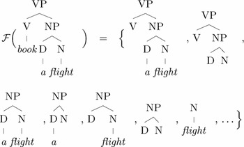
Tree kernels represent trees in terms of their substructures (fragments) which are mapped into feature vector spaces, e.g.,  n. A kernel function measures the similarity between two trees by counting the number of their common fragments. For example, Figure 1 shows some substructures for the parse tree of the sentence ‘book a flight’. The main advantage of tree kernels is that to compute the substructures shared by two trees τ1 and τ2, the whole fragment space is not used. In the following, we report the formal definition presented in Collins and Duffy (Reference Collins and Duffy2002).
A syntactic parse tree.

Given the set of fragments {f 1, f 2,. . . } = , the indicator function Ii(n) is equal to 1 if the target fi is rooted at node n and 0 otherwise. A tree kernel is then defined as

where N τ1 and N τ2 are the sets of the τ1's and τ2's nodes, respectively, and  . The latter is equal to the number of common fragments rooted in the n 1 and n 2 nodes, and Δ can be evaluated with the following algorithm:
(1) if the productions at n 1 and n 2 are different, then Δ(n 1, n 2) = 0;
(2) if the productions at n 1 and n 2 are the same, and n 1 and n 2 have only leaf children (i.e., they are preterminal symbols), then Δ(n 1, n 2) = 1};
(3) if the productions at n 1 and n 2 are the same, and n 1 and n 2 are not pre-terminals, then
(4)
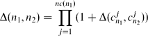
where nc(n 1) is the number of the children of n 1 and cnj is the jth child of the node n. Note that since the productions are the same, nc(n 1) = nc(n 2).
Additionally, we add the decay factor λ by modifying steps (2) and (3) as follows:Footnote 1
(2)
(3)
The computational complexity of (3) is O(|N τ1| × |N τ2|), although the average running time tends to be linear (Moschitti Reference Moschitti2006a).
The next section shows a technique to assign the same placeholders to similar text and hypothesis pair.
3.3.2 Kernel for the ground rule space
Given the above tree kernel functions, the definition of a kernel Ks(〈T, H〉, 〈T′, H′〉) for a ground syntactic rule feature space (i.e., synt) is

Also, the p_cont space can be simply obtained using the product (see Moschitti and Zanzotto Reference Moschitti and Zanzotto2008 for a detailed explanation). Unfortunately (and surprisingly) when huge kernel spaces are multiplied according to the Cartesian product, the resulting number of features is extremely high, and also a robust algorithm like SVMs becomes subject to the curse of high dimensionality. In other words, too many irrelevant features make those relevant ineffective.
The solution of this problem for TE is proposed in Zanzotto and Moschitti (Reference Zanzotto and Moschitti2006) and Moschitti and Zanzotto (Reference Moschitti and Zanzotto2007) and reported in the next section (see (6)). It is possible to showFootnote 2 that placeholders determine a link between the fragments of the text and the hypothesis, which are produced by two distinct tree kernels and merged by the simple kernel sum. This allows us to approximate the paired feature space. The advantage is that only the fragments marked by placeholders (i.e., those very interesting for the target problem) will be paired. This reduced number of feature pairs is easily manageable by SVMs. As we want to compare the synt space with the plac_basic and plac_all, we adopted the same approximation in the computation of the kernel in (5); i.e., we use the sum instead of the product.
3.3.3 Matching placeholder-based features
Defining kernel functions for plac_basic and plac_all is not trivial. Tree kernels applied to two texts or two hypotheses match identical fragments. When placeholders are added to trees as in plac_basic and plac_all, the labeled fragments are matched only if the basic fragments and the assigned placeholders match. For example, let us compare the pair (T 16, H 16) of Section 3.2 with the following (T 10, H 10):
The two pairs share many common features such as
Yet, a simple use of the tree kernel function can lead to missing these common features. In (T 16, H 16)
is

while in (T 17, H 17) it is

. To detect this feature with simple tree kernel functions we need to find a correct mapping between placeholders in (T 16, H 16) and in (T 17, H 17). It is straightforward to note that the correspondences

=
and
=
allow more substructures (i.e., large part of the trees) to be identical.
Although, there may be several approaches to accomplish this task, we apply a basic heuristic which is very intuitive:
Choose the placeholder assignment that maximizes the tree kernel function over all possible correspondences.
More formally, let A and A′ be the placeholder sets of 〈T, H〉 and 〈T′, H′〉, respectively; without loss of generality, we consider |A| ≥ |A′|, and we align a subset of A with A′. The best alignment is the one that maximizes the syntactic and lexical overlapping of the two subtrees induced by the aligned set of anchors. By calling C the set of all bijective mappings from S ⊆ A, with |S| = |A′|, to A′, an element c ∈ C is a substitution function. We define the best alignment c max the one determined by

where (i) t(⋅, c) returns the syntactic tree enriched with placeholders replaced by means of the substitution c, (ii) i is the identity substitution, and (iii) TK(τ1, τ2) is a tree kernel function (e.g., the one specified by (3)) applied to the two trees τ1 and τ2.
At the same time, the desired similarity value to be used in the learning algorithm is given by TK(t(T, cmax), t(T′, i)) + TK(t(H, cmax), t(H′, i), i.e., by solving the following optimization problem:

As a final remark, it should be noted that (a) Ks(〈T, H〉, 〈T′, H′〉) is a symmetric function, since the set of derivation C are always computed with respect to the pair that has the largest anchor set, and (b) it is not a valid kernel, as the max function does not in general produce valid kernels. However, in Haasdonk (Reference Haasdonk2005), it is shown that when kernel functions are not positive semidefinite like in this case, SVMs still solve a data separation problem in pseudo-Euclidean spaces. The drawback is that the solution may be only a local optimum. Nevertheless, such a solution can still be valuable, as the problem is modeled with a very rich feature space.
3.4 Refining cross-pair syntactic similarity
The efficiency of the kernel approach proposed in the previous section should be improved to favor its applicability with SVMs. This can be done by decreasing the computational complexity of (6) and by pruning irrelevant information in large syntactic trees.
Controlling the computational cost. The computational cost of cross-pair similarity between two tree pairs (6) depends on the size of C. This is combinatorial in the size of A and A′, i.e., |C| = (|A| − |A′|)!|A′|! if |A| ≥ |A′|. Thus we should keep the sizes of A and A′ reasonably small.
To reduce the number of placeholders, we consider the notion of chunk defined in Abney (Reference Abney, Bloothooft, Church and Young1996), i.e., not recursive kernels of noun, verb, adjective, and adverb phrases. When placeholders are in a single chunk in both the text and the hypothesis we assign them the same name. The placeholder reduction procedure also gives the possibility of resolving the ambiguity still present in the anchor set A. A way to eliminate the ambiguous anchors is to select those that reduce the final number of placeholders. Finally, in Moschitti and Zanzotto (Reference Moschitti and Zanzotto2007), a more efficient algorithm for computing the kernel Ks is presented together with its training and testing time.
Pruning irrelevant information in large text trees. Often only a portion of the parse trees is relevant to detect entailments. For instance, let us consider the following pair from the RTE1 corpus:
Only the bold part of T supports the implication; the rest is useless and also misleading: if we used it to compute the similarity it would reduce the importance of the relevant part. Moreover, as we normalize the syntactic tree kernel with respect to the size of the two trees, we need to focus only on the part relevant to the implication. The anchored leaves are good indicators of relevant parts, but also some other parts may be very relevant. For example, the function word not plays an important role.
The reduction procedure that we apply can be formally expressed as follows: given a syntactic tree T, the set of its nodes N(t), and a set of anchors, we build a tree t′ with all the nodes N′ that are anchors or ancestors of any anchor. Moreover, we add to t′ the leaf nodes of the original tree T that are direct children of the nodes in N′. We apply such procedure only to the syntactic trees of texts before the computation of the kernel function.
4 Toward a semantic pair feature space
For modeling RTE, plac_basic and plac_all are appealing spaces, as they learn generalized rewrite rules. Unfortunately, these models suffer from a major problem which limits their applicability: they can only learn rules based on syntax and on simple lexical–semantic evidence at the leaf level, while higher levels of semantic information are neglected. In particular, lexical–semantic knowledge is only used to find placeholders, by aligning two semantically similar words. Yet, the semantic relations between words linked by placeholders are not considered in the final models. This limitation causes the algorithm to infer erroneous first-order rewrite rules. Suppose for example that the model leveraging pairs (T 10, H 10) has to learn the following rule:
where the placeholder

anchors buy and own. This rule is useful to classify examples as
where the relation between the two anchored verbs conquer and govern is ‘causation’, as for buy and own. In WordNet (Miller Reference Miller1995), own entails buy as well as govern entails conquer. Yet, the rule will fail when used for
where assassinate and poison are anchored as generically similar verbs. The limitation of the syntactic pair feature spaces is that placeholders do not convey the semantic knowledge needed in cases such as the above, where the semantic relation between connected verbs is essential.
In this section, we show that these models can be easily extended to include shallow semantic information. We present the syntax-semantic pair feature space which solves some of the above limitations by introducing the notion of typed anchors. The idea is to enrich the syntactic trees of text and hypothesis with the relational semantic information standing between anchored words. Operationally, we do so by assigning a semantic tag expressing the semantic relation to placeholders. In the example above, by making explicit the entailment relation own ←buy, we obtain the following correct rule, where the placeholder
is assigned the ← entailment tag:
Of course in case there is no implication between the two verbs we would have a different fragment pair, since the type on
will be different, i.e., →.
Formally, our syntactic–semantic pair feature space is an extension of plac_all, where the trees are now enriched with semantic typed anchors:

where σ enriches fragments with typed anchors. In order to operationally implement the model, we need to solve two issues: (i) decide what type of semantic relations we want to represent in the typed anchors (Section 4.1); (ii) define a policy to encode this information in the tree; i.e., decide at which level(s) of the tree the anchor type must be encoded (Section 4.2).
4.1 Defining anchor types
In the literature, many attempts to introduce semantic information in RTE systems have failed. One of the main reasons for this failure is that any model using semantic information deals with ambiguity. To overcome this issue, we focus on a controlled set of relevant relation types, defined in WordNet: part-of, antinomy, and verb entailment. This controlled set has been chosen because it is relevant for a large part of entailment cases.Footnote 3
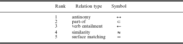
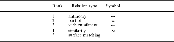
We also define two more general anchor types: similarity and surface matching. The first type links words which are similar according to the WordNet similarity measure described in (Jiang and Conrath Reference Jiang and Conrath1997). This type is intended to capture synonymy and hyponymy. The second type is activated when words or lemmas match, capturing semantically equivalent words. The complete set of relation types used in the experiments is given in Table 1.
Ranked anchor types
4.2 Policies for augmenting placeholders with anchor types
To integrate anchor types in the syntactic tree, the main problem is to decide how the semantic information should be encoded, i.e., where the new typed labels should be most effectively integrated. We experiment with two possible feature space models:
Typed anchor model (ta). Anchor types augment only the preterminal nodes of the syntactic tree;
Propagated typed anchor model (tap). Anchors climb up in the syntactic tree according to some specific climbing-up rules, similar to what done for place-holders.
The ta model is easy to implement: typed anchor simply augment the preterminal nodes of anchored words.
The tap model allows anchor types to climb up in the syntactic tree, repeating the anchor type information in many fragments, which are compared by the tree kernel function. This guarantees that the type information is used in the decision process. The tap model is more complex with respect to ta, as it depends on the strategy adopted for the anchor climbing-up. In particular, the strategy must account for how anchors that climb up to the same node should interact. We implement our strategy by using climbing-up rules as done in the case of placeholders. Yet, in our case rules must consider the semantic information of the typed anchors. The choice of correct climbing-up rules is critical, as an incorrect rule could completely alter the semantics of the tree, as we show in later examples. In the case of placeholders, the climbing-up rule states that a constituent in the syntactic tree takes the placeholder of its semantic head. It is easy to demonstrate that in the case of typed anchors this rule would have disastrous effects. For example, consider the following false entailment pair:
In the example, we apply the above-mentioned rule: the typed anchor =
climbs up to the preterminal node NP, instead of the typed anchor ↔
, as it is the head of the constituent. If modeled in this way, this false entailment pair could generate, among others, the incorrect rewrite rule
which states the following:
if two fragments have the same syntactic structure S(NP, VP(VBZ, NP)), and there is a semantic equivalence (=) on all constituents, then entailment does not hold.
This rule is wrong, as all substructures are semantically equivalent.
The problem is that the wrong typed anchor climbed up the tree: we need the antinomy anchor on the adjective (tall/short) to climb up, instead of the matching anchor on the noun (boy/boy), in order to learn a correct rule. Our strategy must then implement a climbing-up rule producing these trees:
In this case the pair generates correct rewrite rules, such as
The rule states the following: if two fragments have the same syntactic structure S(NP 1, VP(VBZ, NP 2)), and there is an antonym type (↔) on the S and NP 2, then entailment does not hold.
The above example shows that the anchor type that has to climb up depends on the structure of the constituents; thus climbing-up rules depend on the structure. The algorithm to encode such dependency can be very complex. Luckily, this intuition can be also captured by a simpler approximation. Instead of having climbing-up rules for each constituent type, we can rely on a ranking of the anchor types (as the one reported in Table 1). The anchor type that climbs up is the one that has a higher rank. In the example, this strategy produces the correct solution, as antinomy has a higher rank than surface match. We then implement in our model the following climbing-up rule:
Our ordered set  is consistent with common-sense intuitions. In the experimental section we will empirically demonstrate its validity by reporting experiment evidence.
5 Experimental evaluation
In the previous sections, we have defined several feature spaces, and we have shown that plac_basic and plac_all can encode richer and more expressive features than simpler spaces (namely, lex, cont, p_cont, and synt) in SVMs.
Our experiments aim at empirically showing the above claim, where the representation layer used to manually or automatically extract features is constituted by automatically generated parse trees. Moreover, we show that plac_basic and plac_all can be successfully extended with semantic information by creating the new spaces ta and tap.
Our experiments are organized as follows: Section 5.2 shows that plac_basic and plac_all outperforms synt. This suggests that ground syntactic rules learned from synt are less powerful than the first-order rules learnable from plac_basic and plac_all. Unfortunately, the above outcome is less evident when the simple lex is added to the previous models as shown in Section 5.3; the extreme effectiveness of the latter tends to make flat the contribution of the other feature spaces. To support this interpretation, in Section 5.4 we show, by means of learning curves, that plac_basic and plac_all expressing first-order syntactic rules are able to learn from examples, whereas lex reaches immediately a plateau.
Moreover, the first-order-based models used in combination with the similarity features improve the latter. As a final analysis, experimental results in Section 5.5 show that first-order rule feature spaces are also suited for including the semantics of typed anchors (ta and tap).
5.1 Experimental settings
For the experiments, we used the RTE Challenge datasets: RTE1 (Dagan et al. Reference Dagan, Glickman, Magnini, Quiñonero-Candela, Dagan, Magnini and d'Alché-Buc2006), RTE2 (Bar-Haim et al. Reference Bar-Haim, Dagan, Dolan, Ferro, Giampiccolo, Magnini and Szpektor2006), and RTE3 (Giampiccolo et al. Reference Giampiccolo, Magnini, Dagan and Dolan2007). These sets contain respectively 1367, 1600, and 1600 training/testing instances, evenly split between positive and negative examples. The RTE set is the union of the three sets.
We also used the following resources:
• the Charniak parser (Charniak Reference Charniak2000) and the morpha lemmatizer (Minnen, Carroll and Pearce Reference Minnen, Carroll and Pearce2001) to carry out the syntactic and morphological analysis;
• WordNet 2.0 (Miller Reference Miller1995) to extract the verbs in entailment, the derivationally related words, and the antonymous words used both for finding and for typing anchors;
• the wn::similarity package (Pedersen, Patwardhan and Michelizzi Reference Pedersen, Patwardhan and Michelizzi2004) to compute the similarity function for finding anchors between the text T and the hypothesis H and to compute the lexical similarity (lex) in the similarity feature space we used for comparison;
• SVM-light-TKFootnote 4 (Moschitti Reference Moschitti2006b) which encodes the basic tree kernel function, in SVM-light (Joachims Reference Joachims, Schlkopf, Burges and Smola1999).
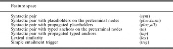
The feature sets used in the experiments are reported in Table 2.
Feature spaces used in the experiments

5.2 First-order versus ground syntactic feature spaces
In a first set of experiments, we compare the two first-order spaces plac_basic and plac_all against the ground space, synt.
We run four different experiments by repeating m times in an n-fold cross-validation on the RTE1, RTE2, and RTE3 and RTE datasets. The results are reported in Table 3: the first column shows the dataset; the second describes the number of folds and the number of times the experiment has been carried out; the third, the fourth, and the last column report the averaged accuracy along with the standard deviation when using synt, plac_basic, and plac_all. The results show the following: (a) The accuracy obtained with plac_all is always significantly better than the accuracy obtained with synt, especially for the RTE2 and the RTE3 sets. (b) In the case of RTE1 and RTE2, the accuracy produced by synt is roughly equal to the one produced by plac_basic. Indeed, plac_basic differs from synt only in the leaves. (Placeholders are assigned only to the preterminal nodes.) In other words, only few fragments contain relational information, i.e., placeholders. We can conclude that a significant improvement can only be observed when moving from plac_basic to plac_all which better describes first-order rules. (c) In the case of RTE3, the assignment of placeholders to preterminal nodes already yields an important improvement (cf. synt with plac_basic).
Mean accuracy and standard deviation within different pair feature spaces: n-fold cross-validations repeated m times

The above results suggest that our spaces are able to model a richer set of rules, thanks to the use of variables. We also claim that such space includes most of the entailment trigger-based features. To show the validity of this statement, we performed an experiment combining synt and plac_all with the simple entailment trigger feature space (trig).
For trig, we used three features representing three different rules, similar to Hickl et al. (Reference Hickl, Williams, Bensley Roberts, Rink, Shi, Magnini and Dagan2006), Imkpen et al. (Reference Inkpen, Kipp., Nastase, Magnini and Dagan2006), and Snow, Vanderwende and Menezes (Reference Snow, Vanderwende and Menezes2006): (1) SVO that tests if T and H share a similar subject–verb–object construct; (2) Apposition that tests if H is a sentence headed by the verb to be and if in T there is an apposition that states H; (3) Anaphora that tests if the SVO sentence in H has a similar wh-sentence in T and if the wh-pronoun may be resolved in T with a word similar to the object or the subject of H.
Results in Table 4 show that synt + trig accuracy is lower than the one of synt, suggesting that the two feature spaces are different, and it is complex to merge them together. In contrast, since the first-order syntactic rule feature space encodes already the first-order rules of trig the accuracy of plac_all + trig is not significantly different from plac_all. (SVMs are very robust to redundant features.)
Mixing syntactic pair feature spaces with entailment trigger feature spaces

5.3 Combining the lexical similarity and the syntactic paired-content feature spaces
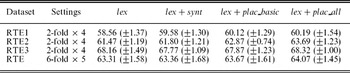
Many studies suggest that lexical overlap is a good heuristic to approximate textual entailment predictions (e.g., Corley and Mihalcea Reference Corley and Mihalcea2005). This section analyzes the interaction between the lexical similarity space (lex) and the basic_plac and plac_all by combining them.
For lex, we used only one feature: the lexical overlap as described in Corley and Mihalcea (Reference Corley and Mihalcea2005), computed by means of WordNet-based similarity between words (i.e., Jiang and Conrath Reference Jiang and Conrath1997) along with the simple token and lemma matching.
The results, reported in Table 5 were obtained with n-fold cross-validation. They show that the accuracy produced by lex alone is close to all mixed feature spaces: first-order rules seem to give no contribution, especially for the RTE3 and RTE datasets. However, by paring the distributions of the fold accuracy generated with the n-fold cross-validation and applying the sign test we found that on the RTE dataset, lex + plac_all is better than lex and lex + synt with 0.005 statistical significance.Footnote 5 This proves that the space using first-order derivations is more accurate than others when used in combination with lexical overlap heuristics.
Experiments mixing the syntactic pair feature space and a simple distance feature space: n-fold cross-validations repeated m times

5.4 When and why to use first-order rule feature spaces
The kind of first-order rules generated with our feature spaces seem to only marginally improve lex. However, this may depend on the small size of the training data. To confirm this hypothesis, we analyzed the learning curves of the different models (Section 5.4.1). Moreover, to show that our models effectively learn first-order rules, we studied them with respect to classes of examples, which can be solved by different classes of rules (Section 5.4.2).
5.4.1 Learning curves
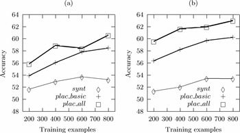
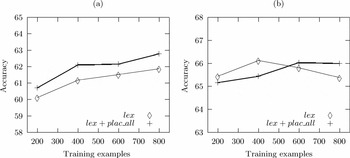
We analyzed four feature spaces: synt, plac_basic, plac_all, and lex. The results for the first three spaces and the fourth space are respectively reported in Figures 2 and 3. We computed the learning curves using the official split in development and test sets of RTE2 and RTE3, where the development set is in turn divided in samples of increasing size with a step of 200 training examples. Each point in the figure is the average accuracy obtained over four runs.Footnote 6
(a) Learning curves over RTE2. (b) Learning curves over RTE3.

Learning curves of lex and lex + plac_all in RTE2 and in RTE3.

Even when all data is used, synt, plac_basic and plac_all do not reach a plateau, meaning that they can improve their accuracy with further data. In contrast, the curves of the lex model (Figure 3) are flat or, in the case of RTE3, decreasing. This is not surprising, since only one parameter has to be learnt, i.e., the threshold; thus the number of needed examples is small. As a final conclusion our first-order feature spaces can really learn from example, whereas the lex model cannot.
5.4.2 Which feature space for which pair?
In this section, we explore how the different feature spaces behave on pairs showing specific phenomena that can be better captured using first-order syntactic rules. For these pairs, plac_all should outperform the other models. We also aim at studying which rule can be learned.
For this purpose, we use the gold standard of entailment examples provided by Vanderwende and Dolan (Reference Vanderwende, Dolan, Candela, Dagan, Magnini and Buc2006). In their study of the RTE1 dataset the authors discovered that 390 pairs out of the 800 of the test set can be classified using solely syntactic cues. Most importantly, entailment examples were clustered in the following four classes (describing the syntactic transformations that hold between texts and hypotheses): (1) syntactic phenomena not involving alternation; (2) syntactic phenomena involving alternation; (3) single word replacement; and (4) lack of syntactic parallelism. Each class is further divided into subclasses, representing specific syntactic transformations rule. For example, the Have-Possessive subclass is a specific type of syntactic phenomenon involving ‘have’ alternation; to be correctly classified, the examples of this category require a model able to handle the first-order transformation rule: X's Y → X has Y.
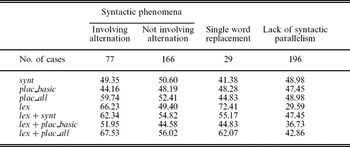
Experimental results of our model over the above dataset are reported in Table 6: the first column reports the feature space; the first row represents the classes of syntactic phenomena in Vanderwende and Dolan (Reference Vanderwende, Dolan, Candela, Dagan, Magnini and Buc2006). The second row shows the number of cases falling in each class according to the manual gold standard (note that examples can belong to more than one class when more than one transformation takes place); and all the other rows illustrate the accuracy of our different models when classifiers are trained on the RTE1 development set.
Accuracy with different feature spaces on specific syntactic phenomena over a portion of the RTE1 test set

The results indicate that placeholders are useful whenever first-order transformation rules are required, i.e., for pairs in the classes syntactic phenomena involving and not involving alternation. In these cases, plac_all outperforms synt and lex + plac_all improves on lex. This is particularly true for the examples showing syntactic phenomena not involving alternation. As expected, in the other two classes of phenomena (single word replacement and lack of syntactic parallelism) RTE is not improved by the use of placeholders, since first-order transformations do not play a relevant role.
By inspecting the above results it is also possible to determine whether or not a specific feature space models a specific rule better than the others, by following the principle that ‘a model which correctly classifies a set of examples clearly requiring a specific first-order transformation most probably encodes such kind of first-order rule’.Footnote 7 For example, if the model correctly classifies active/passive alternations, it likely encodes a rule for active/passive forms. Thus, by noting that plac_all model classifies Be-Appositive, be located-Appositive, and Genitive-Location better than synt, we argue that plac_all can derive such kind of rules better than synt.
5.5 Experiments using typed anchors
In this section we check if first-order syntactic rule feature spaces can be improved by semantic information. Thus, we tested plac_all and its extensions with semantic information, i.e., ta and tap introduced in Section 4.
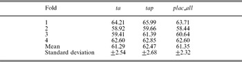
Table 7 reports the accuracy obtained in a 4-fold cross-validation over the RTE2 dataset. The small difference between ta and plac_all accuracy suggests that encoding typed anchors only at the preterminal level is again not sufficient for the generation of effective feature spaces. Thus, such information has to be propagated in the whole syntactic tree. Indeed, the results obtained with tap are significantly higherFootnote 8 than those obtained by plac_all. Therefore, our way of typing anchors with the semantics of word relations is a promising research line for RTE. In general, our results also empirically confirm the findings in Bar-Haim, Szpecktor and Glickman (Reference Bar-Haim, Szpecktor and Glickman2005), which state that lexical and syntactic levels are complementary for RTE.
Experimenting with typed anchors: accuracy results on a 4-fold cross-validation over the RTE2 dataset

6 Conclusion
In this paper, we have proposed the pair content feature space, a novel feature space for RTE that allows ML algorithms to derive first-order rules based on a syntactic–semantic representation of training examples. We have also proposed a method to encode shallow semantic information in data representation through the use of typed anchors. Our model employs variables (represented with placeholders) and linguistic features, as those used in feature structures (Carpenter Reference Carpenter1992).
As a final remark, we observe that several methods for automatically harvesting first-order rewrite rules from large corpora have been recently proposed in the literature, e.g., DIRT (Lin and Pantel Reference Lin and Pantel2001) and TE/ASE (Szpektor et al. Reference Szpektor, Tanev, Dagan and Coppola2004)). These models are complementary to ours, as they are based on a completely different principle (i.e., the distributional hypothesis; Harris Reference Harris, Katz and Fodor1964). While these methods can only extract rules encoding a generic notion of similarity between two textual patterns (e.g., X play Y ~ X win Y), recent extensions (Bhagat, Pantel and Hovy Reference Bhagat, Pantel and Hovy2007; Basili et al. Reference Basili, De Cao, Marocco and Pennacchiotti2007; Pantel et al. Reference Pantel, Bhagat, Coppola, Chklovski and Hovy2007) allow the derivation of more specific directional entailment rules, such as X play Y → X win Y. However, these models cannot learn rewrite rules such as ‘the X VERB Y ↛ X does not VERB Y’, which are instead learned by our model.
Although, several systems tried to leverage large repositories such as DIRT (with limited success; de Salvo Braz et al. Reference de Salvo Braz, Girju, Punyakanok, Roth and Sammons2005b; Raina et al. Reference Raina, Haghighi, Cox, Finkel, Michels, Toutanova, MacCartney, de Marneffe, Christopher and Ng2005), the combined use of the two forms of extracting first-order rewrite rules is a very interesting research line. Pilot experiments using verbs in entailment extracted with the method presented in Zanzotto, Pennacchiotti and Pazienza (Reference Zanzotto, Pennacchiotti and Pazienza2006) and our model have shown promising results.
 .