1 Introduction
The notion of an energy cascade is fundamental in existing theories and predictive models of turbulent flows (Pope Reference Pope2000). For constant-density flows, the Richardson–Kolmogorov phenomenology has been postulated to hold in high-Reynolds-number, locally homogeneous and locally isotropic flows under the ansatz of Kolmogorov’s 1941 theory. A well-known prediction of the theory is the so-called Kolmogorov
 $4/5$
-law, which is one of the few exact relations derivable from the Navier–Stokes equations. The law is valid for turbulent scales within the inertial subrange and describes a scale-invariant energy transfer from large to small scales (a forward cascade). The turbulent dissipation rate,
 $\overline{\unicode[STIX]{x1D716}}$
, is used as a surrogate for the interscale energy transfer rate
 $\unicode[STIX]{x1D6F1}$
(
 $\overline{\unicode[STIX]{x1D716}}\approx -\unicode[STIX]{x1D6F1}$
) in turbulence modelling approaches such as Reynolds-averaged Navier–Stokes (RANS) and large-eddy simulation (LES). The
 $4/5$
-law is only a function of eddy sizes, the ‘scale space’ that links interscale energy transfer to dissipation at each physical spatial point. In flows lacking sufficient separation of scales, inhomogeneities and anisotropy are present, and a generalised
 $4/5$
-law known as the Kármán–Howarth–Monin (K–H–M) equation applies. The origin of the K–H–M equation began with the seminal paper by von Kàrmàn & Howarth (Reference von Kàrmàn and Howarth1938), who derived the equation for homogeneous isotropic turbulence. A more recent account of the full K–H–M equation is found in Hill (Reference Hill2002), where several exact relationships of the second-order velocity structure function are given.
The K–H–M equation describes the transfer of energy in both scale and physical space, with the latter reflecting the spatial development of the underlying flow. Several classes of turbulent flow have been studied using the equation. Casciola et al. (Reference Casciola, Gualtieri, Benzi and Piva2003) analysed intermittency correction of velocity structure functions in shear turbulence using direct numerical simulation (DNS). In Gualtieri et al. (Reference Gualtieri, Casciola, Benzi and Piva2007), the K–H–M approach was used to establish the necessary conditions that the filter scale of a large-eddy simulation must satisfy in order to achieve preservation of statistical properties of the resolved field in homogeneous shear flows. Marati, Casciola & Piva (Reference Marati, Casciola and Piva2004) investigated the energetics of wall turbulence using a DNS dataset and laid down a complete and formally precise description of the dynamics of turbulence in the different regions of the channel flow. Valente & Vassilicos (Reference Valente and Vassilicos2015) looked into the energy cascade in grid-generated non-equilibrium decaying turbulence and demonstrated that the appearance of a
 $-5/3$
power law scaling of the wavenumber or frequency in energy spectra does not necessarily imply a classic Richardson–Kolmogorov cascade. In a follow-up paper, Gomes-Fernandes, Ganapathisubramani & Vassilicos (Reference Gomes-Fernandes, Ganapathisubramani and Vassilicos2015) provided further evidence for this observation by showing that an inverse cascade exists in the production region behind a fractal grid in spite of a well-defined
 $-5/3$
power law over one decade in the streamwise fluctuating velocity spectrum. Further support for this observation is provided by the recent DNS study in the very-near-wake region of a two-dimensional square prism by Alves Portela, Papadakis & Vassilicos (Reference Alves Portela, Papadakis and Vassilicos2017). The scale-by-scale energy budgets in wakes and jets have been reported in Thiesset, Antonia & Danaila (Reference Thiesset, Antonia and Danaila2013) and Danaila, Antonia & Burattini (Reference Danaila, Antonia and Burattini2004) respectively.
A number of experiments have reported observations that are at odds with the Richardson–Kolmogorov formulation because they could imply inverse energy cascades; the word ‘could’ is used because in constant-density flows there are two different physical mechanisms capable of transferring energy upscale. The energy cascade is one of them and the distortion of eddies by mean flow gradients is the other one. A detailed description of these two mechanisms is given in the next section. Chen, Meneveau & Katz (Reference Chen, Meneveau and Katz2006) reported positive mean subgrid-scale dissipation in homogeneous isotropic turbulence subjected to rapid straining–relaxation–destraining cycles; this feature was also observed in a subsequent DNS of the same flow performed by Gualtieri & Meneveau (Reference Gualtieri and Meneveau2010). Multiple experiments have observed negative turbulent kinetic energy (t.k.e.) production, such as those of Liberzon et al. (Reference Liberzon, Lüthi, Guala, Kinzelbach and Tsinober2005) in a rapidly sheared flow near a solid boundary and in a Rayleigh–Bénard convection cell, and Charonko & Prestridge (Reference Charonko and Prestridge2017) in a turbulent dense jet in coflow. While backscattering of energy is known to occur instantaneously in turbulent flows (Meneveau & Katz Reference Meneveau and Katz2000) exhibiting a conventional forward cascade, in these experiments, a net transfer of energy from the fluctuations to the mean flow has occurred in the average sense and therefore poses challenges to modelling. For instance, to model an inverse cascade, a negative turbulent viscosity would be required, and that could cause numerical instabilities. A better physical understanding of the interscale energy transfer is required, and one can use the K–H–M equation to probe into this matter. The K–H–M equation in its present form is not applicable to flows with variable densities (VDs), and a further generalisation to include VD effects is needed.
To understand the physical mechanisms that create negative production in t.k.e., we extend the K–H–M equation to VD flows and apply it to the Charonko & Prestridge (Reference Charonko and Prestridge2017) experiments. In that work, one-point statistical energy budgets of the velocity fluctuations were analysed in detail using simultaneous measurements of both the velocity and the density fields. Variable-density effects were observed to be strong and led to significant differences in the advection, production, transport and dissipation of turbulent kinetic energy,
 $k=\overline{u_{i}^{2}}/2$
. The most pronounced difference occurred at the jet centreline where the t.k.e. production term was negative. Here, we will use the extended K–H–M equation to help to explain these observations. A related use of the two-point statistical formulation of the K–H–M equation is reported in a series of papers by Danaila and coworkers (see Voivenel et al. (Reference Voivenel, Danaila, Varea, Renou and Cazalens2016) and references therein). The group has studied the mixing of turbulent jets with variable viscosities while keeping the fluid density a constant. In Voivenel et al. (Reference Voivenel, Danaila, Varea, Renou and Cazalens2016), a variable viscosity (VV) K–H–M equation was derived and the authors demonstrated an interesting feature of VV flows: the spatial gradients of viscosity are sources of t.k.e.
This paper contains a self-contained derivation of the VD K–H–M equation given in appendix A, and VD effects appear as extra terms in the equation. The constant-density version of the K–H–M equation is recalled briefly in § 2, which is followed by an explanation of the rationale behind the proposed generalisation to VD flows. Section 3 gives the details of the experimental dataset used for analysis. The approximations used to compute various terms in the new K–H–M equation are described. Section 4 describes the scale-by-scale energy transfer and § 5 the energy budget, with conclusions regarding these observations in § 6.
2 The K–H–M equation – the evolution of the second-order velocity structure function
The K–H–M equation is the evolution equation of the ensemble-averaged
 $\overline{(\cdot )}$
scale energy defined by
 $\overline{\unicode[STIX]{x1D6FF}q^{2}}=\overline{(\unicode[STIX]{x1D6FF}u_{i})^{2}}=\overline{[u_{i}(\boldsymbol{x})-u_{i}(\boldsymbol{x}^{\prime })]^{2}}$
, where
 $\boldsymbol{x}$
and
 $\boldsymbol{x}^{\prime }$
are two points in physical space. Its derivation follows from a standard manipulation of the Navier–Stokes equations written down separately for the two points which can be found in, e.g., Gomes-Fernandes et al. (Reference Gomes-Fernandes, Ganapathisubramani and Vassilicos2015) and is therefore not repeated here. The full expression in Cartesian coordinates is given in the following equation and its components are labelled using the terminology in Valente & Vassilicos (Reference Valente and Vassilicos2014):
 $$\begin{eqnarray}\displaystyle & & \displaystyle \displaystyle \frac{\unicode[STIX]{x2202}\overline{\unicode[STIX]{x1D6FF}q^{2}}}{\unicode[STIX]{x2202}t}+\overbrace{\left(\frac{U_{k}+U_{k}^{\prime }}{2}\right)\frac{\unicode[STIX]{x2202}\overline{\unicode[STIX]{x1D6FF}q^{2}}}{\unicode[STIX]{x2202}X_{k}}}^{\text{Advection}\,\,A}+\overbrace{\frac{\unicode[STIX]{x2202}\overline{\unicode[STIX]{x1D6FF}u_{k}\unicode[STIX]{x1D6FF}q^{2}}}{\unicode[STIX]{x2202}r_{k}}}^{\text{Nonlinear transport}\,\unicode[STIX]{x1D6F1}}+\overbrace{\frac{\unicode[STIX]{x2202}\unicode[STIX]{x1D6FF}U_{k}\overline{\unicode[STIX]{x1D6FF}q^{2}}}{\unicode[STIX]{x2202}r_{k}}}^{\text{Linear transport}\,\unicode[STIX]{x1D6F1}_{U}}\nonumber\\ \displaystyle & & \displaystyle \quad =\,-\overbrace{2\overline{\unicode[STIX]{x1D6FF}u_{i}\unicode[STIX]{x1D6FF}u_{k}}\frac{\unicode[STIX]{x2202}\unicode[STIX]{x1D6FF}U_{i}}{\unicode[STIX]{x2202}r_{k}}-\overline{(u_{k}+u_{k}^{\prime })\unicode[STIX]{x1D6FF}u_{i}}\frac{\unicode[STIX]{x2202}\unicode[STIX]{x1D6FF}U_{i}}{\unicode[STIX]{x2202}X_{k}}}^{\text{Production}\,P}\nonumber\\ \displaystyle & & \displaystyle \quad -\,\overbrace{\frac{\unicode[STIX]{x2202}}{\unicode[STIX]{x2202}X_{k}}\left(\frac{\overline{(u_{k}+u_{k}^{\prime })\unicode[STIX]{x1D6FF}q^{2}}}{2}\right)}^{\text{Turbulent transport}\,T}-\overbrace{\frac{2}{\unicode[STIX]{x1D70C}}\frac{\unicode[STIX]{x2202}\overline{\unicode[STIX]{x1D6FF}u_{k}\unicode[STIX]{x1D6FF}p}}{\unicode[STIX]{x2202}X_{k}}}^{\text{Pressure transport}\,T_{p}}\nonumber\\ \displaystyle & & \displaystyle \quad +\,\overbrace{2\unicode[STIX]{x1D708}\frac{\unicode[STIX]{x2202}^{2}\overline{\unicode[STIX]{x1D6FF}q^{2}}}{\unicode[STIX]{x2202}r_{k}^{2}}}^{\text{Viscous diffusion}\,D_{\unicode[STIX]{x1D708}}}+\overbrace{\frac{\unicode[STIX]{x1D708}}{2}\frac{\unicode[STIX]{x2202}^{2}\overline{\unicode[STIX]{x1D6FF}q^{2}}}{\unicode[STIX]{x2202}X_{k}^{2}}}^{\text{Viscous diffusion}\,D_{\boldsymbol{X},\unicode[STIX]{x1D708}}}-\overbrace{2\unicode[STIX]{x1D708}\left[\overline{\left(\frac{\unicode[STIX]{x2202}u_{i}}{\unicode[STIX]{x2202}x_{k}}\right)^{2}}+\overline{\left(\frac{\unicode[STIX]{x2202}u_{i}^{\prime }}{\unicode[STIX]{x2202}x_{k}^{\prime }}\right)^{2}}\right]\unicode[STIX]{x1D716}}^{\text{Dissipation }\,4\overline{\unicode[STIX]{x1D716}}},\end{eqnarray}$$
where
 $\unicode[STIX]{x1D6FF}U_{i}=U_{i}-U_{i}^{\prime }$
,
 $\unicode[STIX]{x1D6FF}u_{i}=u_{i}-u_{i}^{\prime }$
and
 $\unicode[STIX]{x1D6FF}p=p-p^{\prime }$
;
 $U$
refers to the Reynolds-averaged mean velocity and
 $u$
is the fluctuation. Unprimed variables are measured at the point
 $\boldsymbol{x}$
and primed variables are at
 $\boldsymbol{x}^{\prime }$
. The two spatial points are separated by a vector
 $\boldsymbol{r}$
,
 $\boldsymbol{r}=\boldsymbol{x}-\boldsymbol{x}^{\prime }$
, and their centroid is
 $\boldsymbol{X}=(\boldsymbol{x}+\boldsymbol{x}^{\prime })/2$
. Equation (2.1) is a function of both scale and physical space,
 $\boldsymbol{r}$
and
 $\boldsymbol{X}$
, of which the latter is responsible for transport and production of scale energy in spatially developing flows. In homogeneous isotropic flows, the scale energy
 $\overline{\unicode[STIX]{x1D6FF}q^{2}}$
is related to the one-dimensional energy spectrum
 $E(k)$
by the following equation (Davidson Reference Davidson2015, p. 90):
 $$\begin{eqnarray}\displaystyle & \displaystyle \overline{\unicode[STIX]{x1D6FF}q^{2}}\approx \int _{\unicode[STIX]{x03C0}/r}^{\infty }E(k)\,\text{d}k+\frac{r^{2}}{\unicode[STIX]{x03C0}^{2}}\int _{0}^{\unicode[STIX]{x03C0}/r}k^{2}E(k)\,\text{d}k. & \displaystyle\end{eqnarray}$$
The first term on the right-hand side represents the sum of the kinetic energy of all scales smaller than
 $r$
and the second term represents the contribution from the enstrophy
 $|\unicode[STIX]{x1D74E}|^{2}$
where
 $\unicode[STIX]{x1D74E}$
is a vector. For
 $r\gg \unicode[STIX]{x1D702}$
, the Kolmogorov scale, the enstrophy contribution is negligible relative to the kinetic energy. The scale energy is therefore
 $\overline{\unicode[STIX]{x1D6FF}q^{2}}\approx \int _{\unicode[STIX]{x03C0}/r}^{\infty }E(k)\,\text{d}k$
. Using the established power law
 $E(k)\sim k^{-5/3}$
, valid for scales inside the inertial subrange, the ratio of energies between scales that are a factor of two apart, e.g.
 $r$
and
 $r/2$
, is around 3.2. This means that
 $\overline{\unicode[STIX]{x1D6FF}q^{2}}$
is mainly the sum of energies of the first few scales (eddies) smaller than
 $r$
. The kinetic energy of scale
 $r$
contributes approximately 70 % to the sum, and
 $\overline{\unicode[STIX]{x1D6FF}q^{2}}$
can therefore be considered as representative of the energy at
 $r$
. This interpretation breaks down near
 $\unicode[STIX]{x1D702}$
, where the enstrophy contribution overwhelms the kinetic energy contribution, and this should be kept in mind when analysing the dissipative scales. Extension of (2.2) to general flows is straightforward and requires the three-dimensional energy spectrum, but the scale arguments made above still hold.
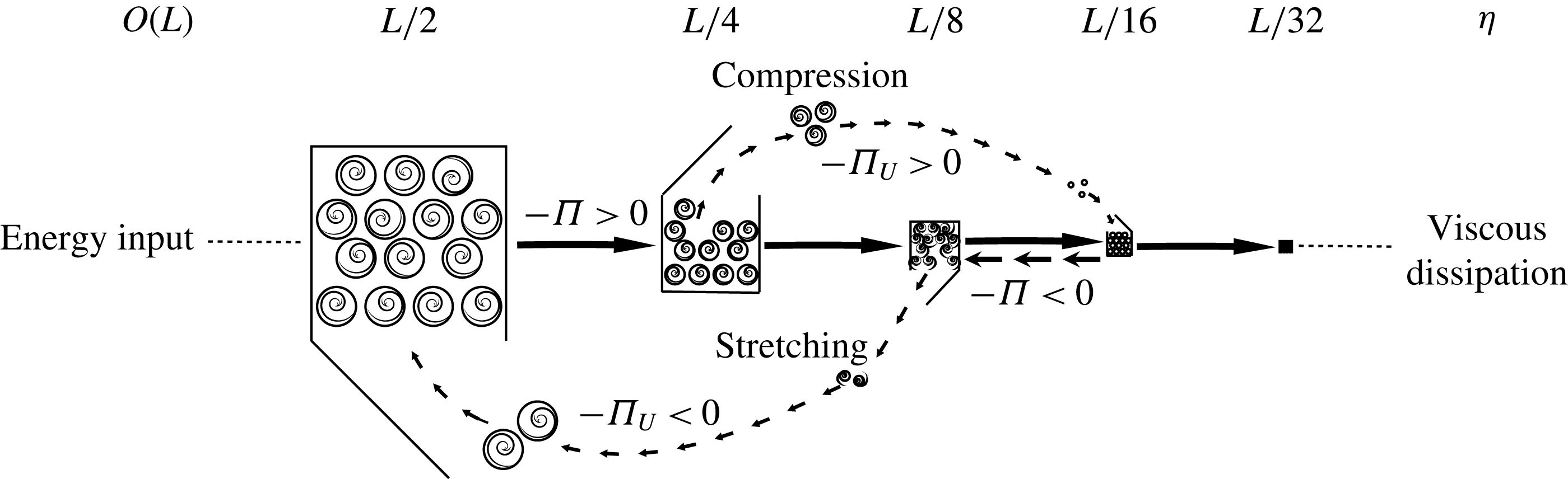
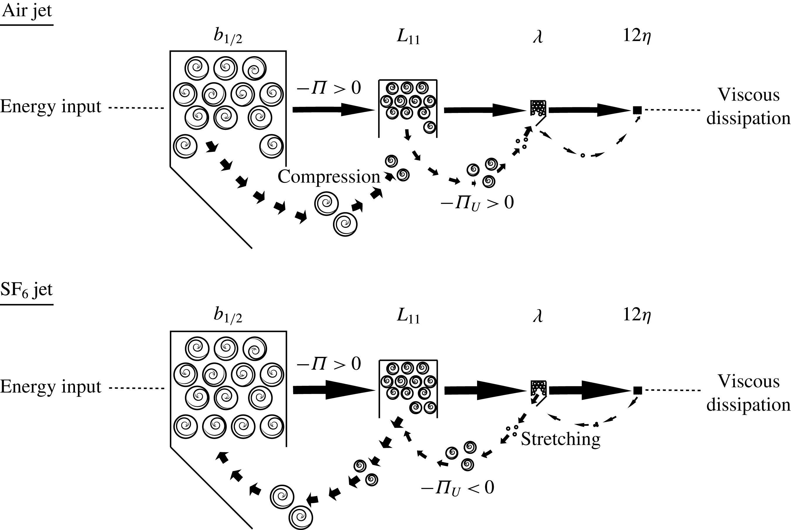
A cartoon illustrating the nature of the linear and nonlinear interscale transfer terms,
 $\unicode[STIX]{x1D6F1}_{U}$
and
 $\unicode[STIX]{x1D6F1}$
. Turbulent kinetic energy in the fluid is created by forcing mechanisms at scales of the order of the integral length scale
 $L$
. This energy is then passed from large to small eddies until it gets converted (dissipated) into internal energy by fluid viscosity at scales of the order of the Kolmogorov length scale
 $\unicode[STIX]{x1D702}$
. Each box in the figure represents one particular eddy size class, starting from
 $L/2$
down to
 $L/32$
. The number density of each size class is represented by the number of eddies inside each box. Here,
 $\unicode[STIX]{x1D6F1}$
is a local process by which scale energy is transferred by turbulent velocity fluctuations between adjacent boxes with their number densities remaining constant during the process;
 $\unicode[STIX]{x1D6F1}_{U}$
, on the contrary, is the distortion of turbulent eddies due to the presence of mean flow gradients
 $\unicode[STIX]{x1D6FF}U$
and in principle can be a non-local process by which scale energy is removed from a particular eddy size class and added to another one that need not be adjacent.

Some of the terms appearing in (2.1) are analogous to the advection
 $A$
, production
 $P$
, turbulent/pressure transport
 $T/T_{p}$
, viscous diffusion
 $D$
and dissipation
 $\overline{\unicode[STIX]{x1D716}}$
terms in the t.k.e. equation, hence their adopted notations. The interscale energy flux terms
 $\unicode[STIX]{x1D6F1}_{U}$
and
 $\unicode[STIX]{x1D6F1}$
are new and they represent the scale-by-scale linear and nonlinear energy flux in
 $\boldsymbol{r}$
-space. Figure 1 shows a mechanistic picture of the roles of
 $\unicode[STIX]{x1D6F1}_{U}$
and
 $\unicode[STIX]{x1D6F1}$
in the energy transfer process among different turbulent eddy size classes in three-dimensional turbulent flows. Turbulent kinetic energy is injected into the fluid by forcing at scales of the order of the integral length scale
 $L$
. This energy is passed down from large to small eddies until it is dissipated into heat by fluid viscosity at scales of the order of the Kolmogorov length scale
 $\unicode[STIX]{x1D702}$
. Successive eddy size classes differing by a factor of two from
 $L/2$
to
 $L/32$
are represented by boxes of different sizes, and the number density of each class is represented by the number of eddies drawn inside the box. The role of
 $\unicode[STIX]{x1D6F1}$
is to transfer scale energy from one size class to immediate neighbours. This local nature of energy transfer in the scale space is a fundamental postulate in the Richardson–Kolmogorov phenomenology and has found substantial support in the very recent DNS study of three-dimensional homogeneous turbulence (
 $Re_{\unicode[STIX]{x1D706}}=315$
and
 $\unicode[STIX]{x1D6F1}_{U}$
is identically zero) reported by Cardesa, Vela-Martin & Jimenez (Reference Cardesa, Vela-Martin and Jimenez2017). These authors tracked the birth and death of eddies and showed that eddies of a given scale originate from eddies twice their scale, whereas they give rise to eddies half their scale before disappearing. In contrast,
 $\unicode[STIX]{x1D6F1}_{U}$
represents the energy loss/gain at a particular eddy size class due to the distortion of the eddy, including changes in size and orientation, by mean flow gradient
 $\unicode[STIX]{x1D6FF}U$
; this can be seen by writing
 $\unicode[STIX]{x1D6F1}_{U}=(\unicode[STIX]{x2202}\unicode[STIX]{x1D6FF}U_{k}\overline{\unicode[STIX]{x1D6FF}q^{2}})/\unicode[STIX]{x2202}r_{k}=\overline{\unicode[STIX]{x1D6FF}q^{2}}(\unicode[STIX]{x2202}\unicode[STIX]{x1D6FF}U_{k}/\unicode[STIX]{x2202}r_{k})+\unicode[STIX]{x1D6FF}U_{k}(\unicode[STIX]{x2202}\overline{\unicode[STIX]{x1D6FF}q^{2}}/\unicode[STIX]{x2202}r_{k})$
. This process is represented in figure 1 by the removal of eddies (circles in a box) from the size class
 $L/4$
to the size class
 $L/16$
; the eddies are compressed by
 $\unicode[STIX]{x1D6FF}U$
. Because
 $\unicode[STIX]{x1D6FF}U$
is flow-dependent,
 $\unicode[STIX]{x1D6F1}_{U}$
is, in principle, a non-local process and is therefore very different in nature from
 $\unicode[STIX]{x1D6F1}$
. In this sense,
 $\unicode[STIX]{x1D6F1}_{U}$
is not an energy cascade postulated in the Richardson–Kolmogorov phenomenology. To distinguish this significant difference between
 $\unicode[STIX]{x1D6F1}_{U}$
and
 $\unicode[STIX]{x1D6F1}$
, we will use ‘transfer’ to refer to the energy loss/gain at a particular scale by the linear term
 $\unicode[STIX]{x1D6F1}_{U}$
, and ‘energy cascade’ is reserved for the nonlinear term
 $\unicode[STIX]{x1D6F1}$
throughout this paper.
Under the assumptions of local equilibrium and homogeneity for scales in the inertial subrange, (2.1) simplifies to the following:
 $$\begin{eqnarray}\displaystyle & \displaystyle \frac{\unicode[STIX]{x2202}\overline{\unicode[STIX]{x1D6FF}u_{k}\unicode[STIX]{x1D6FF}q^{2}}}{\unicode[STIX]{x2202}r_{k}}\approx -2\unicode[STIX]{x1D708}\left[\overline{\left(\frac{\unicode[STIX]{x2202}u_{i}}{\unicode[STIX]{x2202}x_{k}}\right)^{2}}+\overline{\left(\frac{\unicode[STIX]{x2202}u_{i}^{\prime }}{\unicode[STIX]{x2202}x_{k}^{\prime }}\right)^{2}}\right]=-4\overline{\unicode[STIX]{x1D716}}. & \displaystyle\end{eqnarray}$$
This describes the nonlinear energy transfer of fluctuating energy from spherical shells centred at
 $\boldsymbol{X}$
with radius
 $r$
to either spherical shells centred at the same
 $\boldsymbol{X}$
but with different radius or within the same spherical shell but to a different orientation
 $\boldsymbol{r}/r$
(Valente & Vassilicos Reference Valente and Vassilicos2015). Equation (2.3) is a first-order partial differential equation with a non-homogeneous source term on the right. This means that once the dissipation is specified in the interior and on the boundaries of the domain (
 $\boldsymbol{r}$
-space), the equation evolves accordingly and the dynamics is independent of the geometry, inhomogeneity and anisotropy of the large scales insofar as they only set the dissipation rate (Davidson Reference Davidson2015). This is the crux of Richardson–Kolmogorov cascade and is postulated to be universal for any flow. It can be further simplified by assuming local isotropy and by integration over a sphere of radius
 $r$
, resulting in
 $\overline{\unicode[STIX]{x1D6FF}\boldsymbol{u}_{||}\unicode[STIX]{x1D6FF}q^{2}}\approx -(4/3)\overline{\unicode[STIX]{x1D716}}r$
, and from which the
 $4/5$
-law for the longitudinal velocity third-order structure function can be derived, e.g. Monin & Yaglom (Reference Monin and Yaglom1975) and Rasmussen (Reference Rasmussen1999).
The spatial flux term
 $T=-(\unicode[STIX]{x2202}/\unicode[STIX]{x2202}X_{k})(\overline{(u_{k}+u_{k}^{\prime })\unicode[STIX]{x1D6FF}q^{2}}/2)$
of (2.1) represents the transfer of scale energy in the physical space
 $\boldsymbol{X}$
by the fluctuating velocities. It serves to supply scale energy to regions where the production of energy is low, effectively sustaining turbulence in those regions. Examples are the bulk region near the centreline of a channel (Marati et al.
Reference Marati, Casciola and Piva2004) or the edges of a turbulent jet (Charonko & Prestridge Reference Charonko and Prestridge2017).
2.1 An alternative form of (2.1) with local isotropy
An alternative form of the general K–H–M equation, (2.1), is obtained when one carries out an integration over a sphere of radius
 $r=|\boldsymbol{r}|$
and assumes local isotropy. For illustration purposes, we consider the simplified equation (2.3) for homogeneous and locally isotropic flows (see also Gomes-Fernandes et al.
Reference Gomes-Fernandes, Ganapathisubramani and Vassilicos2015), and this gives
 $$\begin{eqnarray}\displaystyle & \displaystyle -\overline{\unicode[STIX]{x1D6FF}u_{1}\unicode[STIX]{x1D6FF}q^{2}}+2\unicode[STIX]{x1D708}\frac{\text{d}\overline{\unicode[STIX]{x1D6FF}q^{2}}}{\text{d}r}=\frac{4}{3}\overline{\unicode[STIX]{x1D716}}r, & \displaystyle\end{eqnarray}$$
where
 $\unicode[STIX]{x1D6FF}u_{1}$
is the streamwise velocity increment and the second term is the integrated form of
 $D_{\unicode[STIX]{x1D708}}$
, which is the viscous contribution to the balance. This equation is valid across both inertial and dissipative subranges under the tenets of Kolmogorov’s 1941 (K41) theory. An obvious limitation is clearly the restriction of isotropy, which is relevant to laboratory flows having small to moderate Taylor–Reynolds number (
 ${<}1000$
, Shen & Warhaft (Reference Shen and Warhaft2000)). Moreover, in situations where K41 does not apply, it hides the directional dependence of the interscale energy flux, in which localised regions in the
 $\boldsymbol{r}$
-space exhibiting an inverse energy cascade cannot be seen (see figures 16 and 17 in Gomes-Fernandes et al. (Reference Gomes-Fernandes, Ganapathisubramani and Vassilicos2015)). Nonetheless, this form has a clear advantage in experimental measurements performed with hot-wire anemometry in that structure functions need only be measured along the streamwise direction instead of over a volume. Extensions of the equation to include large-scale inhomogeneities that bring decay, production and transport to the scale energy have been made in jets by Burattini, Antonia & Danaila (Reference Burattini, Antonia and Danaila2005), wakes by Thiesset et al. (Reference Thiesset, Antonia and Danaila2013) and grid turbulence by Danaila et al. (Reference Danaila, Antonia and Burattini2004), to name a few. Very recently, Sadeghi published two papers (Sadeghi, Lavoie & Pollard Reference Sadeghi, Lavoie and Pollard2015, Reference Sadeghi, Lavoie and Pollard2016) on equilibrium similarity solutions of the scale energy equation of constant-density turbulent round jets. Because the present analysis utilises the full K–H–M equation, scale-by-scale energy budgets derived in previous works can differ from the present analysis at the large scales. The discrepancies, however, are deemed to be small in the inertial and dissipative range where the assumption of local isotropy holds approximately.
2.2 Extension to VD flows
When writing statistical equations for VD flows, the representation of correlations involving density fluctuations is not unique (Chassaing et al.
Reference Chassaing, Antonia, Anselmet, Joly and Sarkar2002). We adopt the Favre-averaged (mass-weighted) formalism because the resulting equations resemble their constant-density counterparts; the Favre decomposition of an instantaneous variable mirrors the Reynolds decomposition. This allows one to recognise the original K–H–M equation in the new VD equation when density is a constant. As detailed in appendix A, a new notation is used for VD flows which is different from the notation in (2.1). Using Favre-averaging, the instantaneous velocities at two separate spatial points
 $\boldsymbol{x}$
and
 $\boldsymbol{x}^{\prime }$
can be written as
 $u_{i}(\boldsymbol{x})=\text{}\underline{U_{i}}+\text{}\underline{u_{i}^{\prime }}=\tilde{\text{}\underline{U_{i}}}+\text{}\underline{u_{i}^{\prime \prime }}$
and
 $u_{i}(\boldsymbol{x}^{\prime })=\text{}\underline{\text{}\underline{U_{i}}}+\text{}\underline{\text{}\underline{u_{i}^{\prime }}}=\tilde{\text{}\underline{\text{}\underline{U_{i}}}}+\text{}\underline{\text{}\underline{u_{i}^{\prime \prime }}}$
. A tilde denotes a Favre-averaged quantity,
 $\tilde{\unicode[STIX]{x1D719}}=\overline{\unicode[STIX]{x1D70C}\unicode[STIX]{x1D719}}/\overline{\unicode[STIX]{x1D70C}}$
, and
 $\unicode[STIX]{x1D719}^{\prime \prime }$
is the remaining Favrian fluctuation. Similarly, the densities at the two points are written as
 $\unicode[STIX]{x1D70C}(\boldsymbol{x})=\text{}\underline{\unicode[STIX]{x1D70C}}$
and
 $\unicode[STIX]{x1D70C}(\boldsymbol{x}^{\prime })=\text{}\underline{\text{}\underline{\unicode[STIX]{x1D70C}}}$
.
The first step is to express the scale energy with a VD formulation. A naive extension of the scale energy
 $\overline{\unicode[STIX]{x1D6FF}q^{2}}=\overline{(\unicode[STIX]{x1D6FF}u_{i})^{2}}$
(old notation) to VD flows would be
 $\overline{(\unicode[STIX]{x1D6FF}\unicode[STIX]{x1D70C}u_{i}^{\prime \prime })^{2}}=\overline{(\text{}\underline{\unicode[STIX]{x1D70C}}\,\text{}\underline{u_{i}^{\prime \prime }}-\text{}\underline{\text{}\underline{\unicode[STIX]{x1D70C}}}\,\text{}\underline{\text{}\underline{u_{i}^{\prime \prime }}})^{2}}$
. However, this brings density-squared terms that have no obvious physical interpretations. Instead, we consider a VD analogue of
 $\overline{(\unicode[STIX]{x1D6FF}u_{i}^{\prime })^{2}}=\overline{\text{}\underline{u_{i}^{\prime 2}}}+\overline{\text{}\underline{\text{}\underline{u_{i}^{\prime 2}}}}-2\overline{\text{}\underline{u_{i}^{\prime }}\text{}\underline{\text{}\underline{u_{i}^{\prime }}}}$
(new notation) that shows that the scale energy in constant-density flows is related to the Reynolds stresses at the two points and the two-point Reynolds stress correlation. The VD analogue should reduce to
 $\overline{(\unicode[STIX]{x1D6FF}u_{i}^{\prime })^{2}}$
when
 $\unicode[STIX]{x1D70C}$
is constant, and a possible candidate is given as follows:
 $$\begin{eqnarray}\displaystyle & \displaystyle \overline{\text{}\underline{\unicode[STIX]{x1D70C}}\text{}\underline{u_{i}^{\prime \prime 2}}}+\overline{\text{}\underline{\text{}\underline{\unicode[STIX]{x1D70C}}}\text{}\underline{\text{}\underline{u_{i}^{\prime \prime 2}}}}-2\left({\textstyle \frac{1}{2}}\overline{[\text{}\underline{\unicode[STIX]{x1D70C}}+\text{}\underline{\text{}\underline{\unicode[STIX]{x1D70C}}}]\text{}\underline{u_{i}^{\prime \prime }}\text{}\underline{\text{}\underline{u_{i}^{\prime \prime }}}}\right), & \displaystyle\end{eqnarray}$$
where
 $\overline{\text{}\underline{\unicode[STIX]{x1D70C}}\text{}\underline{u_{i}^{\prime \prime }}\text{}\underline{u_{j}^{\prime \prime }}}$
is the single-point stress tensor in VD flows at
 $\boldsymbol{x}$
. The last term,
 $(1/2)\overline{[\text{}\underline{\unicode[STIX]{x1D70C}}+\text{}\underline{\text{}\underline{\unicode[STIX]{x1D70C}}}]\text{}\underline{u_{i}^{\prime \prime }}\text{}\underline{\text{}\underline{u_{i}^{\prime \prime }}}}$
, is the two-point stress tensor defined in Clark & Spitz (Reference Clark and Spitz2005) and Clark (Reference Clark2015). A simple algebraic manipulation shows that this form reduces to
 $\overline{(\unicode[STIX]{x1D6FF}u_{i}^{\prime })^{2}}$
by setting
 $\unicode[STIX]{x1D70C}=$
constant and by recalling that the Favre fluctuation is equal to the Reynolds fluctuation (
 $u_{i}^{\prime \prime }=u_{i}^{\prime }$
) when
 $\unicode[STIX]{x1D70C}=$
constant. The above expression can be rewritten in a form similar to
 $\overline{(\unicode[STIX]{x1D6FF}u_{i}^{\prime })^{2}}$
,
 $$\begin{eqnarray}\displaystyle & \displaystyle \overline{(\unicode[STIX]{x1D6FF}u_{i}^{\prime \prime })_{\unicode[STIX]{x1D70C}}^{2}}=\overline{(\text{}\underline{u_{i}^{\prime \prime }}-\text{}\underline{\text{}\underline{u_{i}^{\prime \prime }}})(\text{}\underline{\unicode[STIX]{x1D70C}}\text{}\underline{u_{i}^{\prime \prime }}-\text{}\underline{\text{}\underline{\unicode[STIX]{x1D70C}}}\text{}\underline{\text{}\underline{u_{i}^{\prime \prime }}})}=\overline{\unicode[STIX]{x1D6FF}(u_{i}^{\prime \prime })\unicode[STIX]{x1D6FF}(\unicode[STIX]{x1D70C}u_{i}^{\prime \prime })}. & \displaystyle\end{eqnarray}$$
This is the correct definition of the scale energy in VD flows whose transport equation can be derived from those of the single- and two-point stress tensors. As derived in appendix A, the full equation is
 $$\begin{eqnarray}\displaystyle & & \displaystyle \hspace{-10.00002pt}\displaystyle \frac{\unicode[STIX]{x2202}\overline{(\unicode[STIX]{x1D6FF}u_{i}^{\prime \prime })_{\unicode[STIX]{x1D70C}}^{2}}}{\unicode[STIX]{x2202}t}+\overbrace{{\displaystyle \frac{(\text{}\underline{\tilde{U_{k}}}+\text{}\underline{\text{}\underline{\tilde{U_{k}}}})}{2}}{\displaystyle \frac{\unicode[STIX]{x2202}\overline{(\unicode[STIX]{x1D6FF}u_{i}^{\prime \prime })_{\unicode[STIX]{x1D70C}}^{2}}}{\unicode[STIX]{x2202}X_{k}}}}^{\text{Advection},A}+\overbrace{{\displaystyle \frac{\unicode[STIX]{x2202}\overline{\unicode[STIX]{x1D6FF}u_{k}^{\prime \prime }(\unicode[STIX]{x1D6FF}u_{i}^{\prime \prime })_{\unicode[STIX]{x1D70C}}^{2}}}{\unicode[STIX]{x2202}r_{k}}}}^{\text{Nonlinear transport},\unicode[STIX]{x1D6F1}}+\overbrace{{\displaystyle \frac{\unicode[STIX]{x2202}\unicode[STIX]{x1D6FF}\tilde{U_{k}}\overline{(\unicode[STIX]{x1D6FF}u_{i}^{\prime \prime })_{\unicode[STIX]{x1D70C}}^{2}}}{\unicode[STIX]{x2202}r_{k}}}}^{\text{Linear transport},\unicode[STIX]{x1D6F1}_{U}}\nonumber\\ \displaystyle & & \displaystyle \quad =\,-\overbrace{2[\unicode[STIX]{x1D608}_{ik}+\unicode[STIX]{x1D609}_{ik}]{\displaystyle \frac{\unicode[STIX]{x2202}\unicode[STIX]{x1D6FF}\tilde{U_{i}}}{\unicode[STIX]{x2202}r_{k}}}-[\unicode[STIX]{x1D608}_{ik}-\unicode[STIX]{x1D609}_{ik}]{\displaystyle \frac{\unicode[STIX]{x2202}\unicode[STIX]{x1D6FF}\tilde{U_{i}}}{\unicode[STIX]{x2202}X_{k}}}}^{\text{Production},P}-\overbrace{{\displaystyle \frac{1}{2}}{\displaystyle \frac{\unicode[STIX]{x2202}\overline{(\text{}\underline{u_{k}^{\prime \prime }}+\text{}\underline{\text{}\underline{u_{k}^{\prime \prime }}})(\unicode[STIX]{x1D6FF}u_{i}^{\prime \prime })_{\unicode[STIX]{x1D70C}}^{2}}}{\unicode[STIX]{x2202}X_{k}}}}^{\text{Turbulent transport},T}\nonumber\\ \displaystyle & & \displaystyle \quad -\,\overbrace{\Bigg\{\overline{[1+\text{}\underline{\unicode[STIX]{x1D70C}}/\text{}\underline{\text{}\underline{\unicode[STIX]{x1D70C}}}]{\displaystyle \frac{\unicode[STIX]{x2202}(\text{}\underline{p^{\prime }}-\text{}\underline{\text{}\underline{p^{\prime }}})}{\unicode[STIX]{x2202}\text{}\underline{\text{}\underline{x_{i}}}}}+2{\displaystyle \frac{\unicode[STIX]{x2202}(\text{}\underline{p^{\prime }}-\text{}\underline{\text{}\underline{p^{\prime }}})}{\unicode[STIX]{x2202}\text{}\underline{x_{i}}}}\Bigg\}\text{}\underline{u_{i}^{\prime \prime }}}+\Bigg\{\overline{[1+\text{}\underline{\text{}\underline{\unicode[STIX]{x1D70C}}}/\text{}\underline{\unicode[STIX]{x1D70C}}]{\displaystyle \frac{\unicode[STIX]{x2202}(\text{}\underline{p^{\prime }}-\text{}\underline{\text{}\underline{p^{\prime }}})}{\unicode[STIX]{x2202}\text{}\underline{x_{i}}}}+2{\displaystyle \frac{\unicode[STIX]{x2202}(\text{}\underline{p^{\prime }}-\text{}\underline{\text{}\underline{p^{\prime }}})}{\unicode[STIX]{x2202}\text{}\underline{\text{}\underline{x_{i}}}}}\Bigg\}\text{}\underline{\text{}\underline{u_{i}^{\prime \prime }}}}}^{\text{Pressure transport},T_{p}}\nonumber\\ \displaystyle & & \displaystyle \quad +\,\overbrace{2\unicode[STIX]{x1D707}\Bigg\{\overline{{\displaystyle \frac{\unicode[STIX]{x2202}}{\unicode[STIX]{x2202}\text{}\underline{x_{k}}}}\Bigg[(\unicode[STIX]{x1D6FF}u_{i}^{\prime }){\displaystyle \frac{\unicode[STIX]{x2202}(\text{}\underline{u_{i}^{\prime }}-\text{}\underline{\text{}\underline{u_{i}^{\prime }}})}{\unicode[STIX]{x2202}\text{}\underline{x_{k}}}}\Bigg]+{\displaystyle \frac{\unicode[STIX]{x2202}}{\unicode[STIX]{x2202}\text{}\underline{\text{}\underline{x_{k}}}}}\Bigg[(\unicode[STIX]{x1D6FF}u_{i}^{\prime }){\displaystyle \frac{\unicode[STIX]{x2202}(\text{}\underline{u_{i}^{\prime }}-\text{}\underline{\text{}\underline{u_{i}^{\prime }}})}{\unicode[STIX]{x2202}\text{}\underline{\text{}\underline{x_{k}}}}}\Bigg]}\Bigg\}}^{\text{Viscous diffusion},D_{\unicode[STIX]{x1D708}}+D_{\boldsymbol{X},\unicode[STIX]{x1D708}}}\nonumber\\ \displaystyle & & \displaystyle \quad -\,\overbrace{2\unicode[STIX]{x1D707}\left\{\overline{\left({\displaystyle \frac{\unicode[STIX]{x2202}\text{}\underline{u_{i}^{\prime }}}{\unicode[STIX]{x2202}\text{}\underline{x_{k}}}}\right)\left({\displaystyle \frac{\unicode[STIX]{x2202}\text{}\underline{u_{i}^{\prime }}}{\unicode[STIX]{x2202}\text{}\underline{x_{k}}}}\right)}+\overline{\left({\displaystyle \frac{\unicode[STIX]{x2202}\text{}\underline{\text{}\underline{u_{i}^{\prime }}}}{\unicode[STIX]{x2202}\text{}\underline{\text{}\underline{x_{k}}}}}\right)\left({\displaystyle \frac{\unicode[STIX]{x2202}\text{}\underline{\text{}\underline{u_{i}^{\prime }}}}{\unicode[STIX]{x2202}\text{}\underline{\text{}\underline{x_{k}}}}}\right)}\right\}\unicode[STIX]{x1D716}}^{\text{Dissipation},4\overline{\unicode[STIX]{x1D716}}}+\underbrace{\overline{{\displaystyle \frac{\unicode[STIX]{x0394}\unicode[STIX]{x1D70C}}{\text{}\underline{\unicode[STIX]{x1D70C}}}}\text{}\underline{\text{}\underline{u_{i}^{\prime \prime }}}{\displaystyle \frac{\unicode[STIX]{x2202}\text{}\underline{\unicode[STIX]{x1D70F}_{ik}^{\prime }}}{\unicode[STIX]{x2202}\text{}\underline{x_{k}}}}}-\overline{{\displaystyle \frac{\unicode[STIX]{x0394}\unicode[STIX]{x1D70C}}{\text{}\underline{\text{}\underline{\unicode[STIX]{x1D70C}}}}}\text{}\underline{u_{i}^{\prime \prime }}{\displaystyle \frac{\unicode[STIX]{x2202}\text{}\underline{\text{}\underline{\unicode[STIX]{x1D70F}_{ik}^{\prime }}}}{\unicode[STIX]{x2202}\text{}\underline{\text{}\underline{x_{k}}}}}}}_{\text{VD effects},\unicode[STIX]{x1D707}\unicode[STIX]{x0394}\unicode[STIX]{x1D70C}}\nonumber\\ \displaystyle & & \displaystyle \quad +\,\underbrace{2\{\text{}\underline{a_{i}}-a_{i}(\boldsymbol{x}^{\prime },\boldsymbol{x})\}{\displaystyle \frac{\unicode[STIX]{x2202}\text{}\underline{\overline{P}}}{\unicode[STIX]{x2202}\text{}\underline{x_{i}}}}+2\{\text{}\underline{\text{}\underline{a_{i}}}-a_{i}(\boldsymbol{x},\boldsymbol{x}^{\prime })\}{\displaystyle \frac{\unicode[STIX]{x2202}\text{}\underline{\text{}\underline{\overline{P}}}}{\unicode[STIX]{x2202}\text{}\underline{\text{}\underline{x_{i}}}}}}_{\text{Mass-flux{-}pressure},a_{P}}\nonumber\\ \displaystyle & & \displaystyle \quad -\,\underbrace{2\{\text{}\underline{a_{i}}-a_{i}(\boldsymbol{x}^{\prime },\boldsymbol{x})\}{\displaystyle \frac{\unicode[STIX]{x2202}\text{}\underline{\overline{\unicode[STIX]{x1D70F}_{ik}}}}{\unicode[STIX]{x2202}\text{}\underline{x_{k}}}}-2\{\text{}\underline{\text{}\underline{a_{i}}}-a_{i}(\boldsymbol{x},\boldsymbol{x}^{\prime })\}{\displaystyle \frac{\unicode[STIX]{x2202}\text{}\underline{\text{}\underline{\overline{\unicode[STIX]{x1D70F}_{ik}}}}}{\unicode[STIX]{x2202}\text{}\underline{\text{}\underline{x_{k}}}}}}_{\text{Mass-flux{-}stress},a_{\unicode[STIX]{x1D70F}}}\nonumber\\ \displaystyle & & \displaystyle \quad -\,\underbrace{\{\unicode[STIX]{x1D61B}_{ii}(\boldsymbol{x},\boldsymbol{x}^{\prime })+\unicode[STIX]{x1D61B}_{ii}(\boldsymbol{x}^{\prime },\boldsymbol{x})\}}_{T_{VD}}-\underbrace{2\left\{{\displaystyle \frac{Q_{i}(\boldsymbol{x},\boldsymbol{x}^{\prime })}{\text{}\underline{\text{}\underline{\overline{\unicode[STIX]{x1D70C}}}}}}{\displaystyle \frac{\unicode[STIX]{x2202}\text{}\underline{\text{}\underline{\unicode[STIX]{x1D619}_{ik}}}}{\unicode[STIX]{x2202}\text{}\underline{\text{}\underline{x_{k}}}}}+{\displaystyle \frac{Q_{i}(\boldsymbol{x}^{\prime },\boldsymbol{x})}{\text{}\underline{\overline{\unicode[STIX]{x1D70C}}}}}{\displaystyle \frac{\unicode[STIX]{x2202}\text{}\underline{\unicode[STIX]{x1D619}_{ik}}}{\unicode[STIX]{x2202}\text{}\underline{x_{k}}}}\right\}}_{Q}.\hspace{-10.00002pt}\end{eqnarray}$$
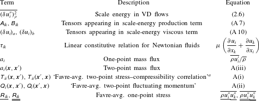
Table 1 provides a reference for the various terms appearing in (2.7), many of which are defined in appendix A. By setting
 $\tilde{U_{i}}=\overline{U_{i}}$
and
 $u_{i}^{\prime \prime }=u_{i}^{\prime }$
, the
 $A$
,
 $\unicode[STIX]{x1D6F1}$
,
 $\unicode[STIX]{x1D6F1}_{U}$
,
 $T$
and
 $4\overline{\unicode[STIX]{x1D716}}$
terms revert to their constant-density counterparts. With a little more algebra, the
 $P$
,
 $T_{p}$
,
 $D_{\unicode[STIX]{x1D708}}$
and
 $D_{\boldsymbol{X},\unicode[STIX]{x1D708}}$
terms will also behave similarly. The remaining five terms,
 $\unicode[STIX]{x1D707}\unicode[STIX]{x0394}\unicode[STIX]{x1D70C}$
,
 $a_{P},a_{\unicode[STIX]{x1D70F}},T_{VD}$
and
 $Q$
, arise due to VD effects. When
 $\unicode[STIX]{x1D70C}=$
constant, they drop out from the equation and one recovers the original K–H–M equation.
Descriptions of terms appearing in the VD K–H–M equation (2.7). The fluid is assumed to be incompressible.

a
Different from the two-point stress tensor
 $\unicode[STIX]{x1D619}_{ii}(\boldsymbol{x},\boldsymbol{x}^{\prime })=(\overline{[\text{}\underline{\unicode[STIX]{x1D70C}}+\text{}\underline{\text{}\underline{\unicode[STIX]{x1D70C}}}]\text{}\underline{u_{i}^{\prime \prime }}\text{}\underline{\text{}\underline{u_{i}^{\prime \prime }}}})/2$
(Clark Reference Clark2015).
2.3 The Kolmogorov
 $4/5$
-law in VD flows

In homogeneous and local-equilibrium flows, (2.7) admits the VD analogue of the constant-density Kolmogorov equation ((2.3), with the viscous diffusion term included),
 $$\begin{eqnarray}\displaystyle & \displaystyle \unicode[STIX]{x1D6F1}=D_{\unicode[STIX]{x1D708}}+D_{\boldsymbol{X},\unicode[STIX]{x1D708}}-4\overline{\unicode[STIX]{x1D716}}+(\unicode[STIX]{x1D707}\unicode[STIX]{x0394}\unicode[STIX]{x1D70C}+a_{P}+a_{\unicode[STIX]{x1D70F}}-T_{VD}-Q). & \displaystyle\end{eqnarray}$$
It contains the extra five terms due to VD effects. Because the
 $4\overline{\unicode[STIX]{x1D716}}$
term has the same form as its counterpart in constant-density flows (see (2.1)),
 $\overline{\unicode[STIX]{x1D716}}$
will have a constant prefactor of
 $4/5$
when an integration over a sphere of radius
 $r=|\boldsymbol{r}|$
under the assumption of local isotropy is first carried out on (2.8). After further algebraic manipulations using several vector identities derived from the Navier–Stokes equations, one obtains the
 $4/5$
prefactor. A detailed description of the procedures involved is given by Rasmussen (Reference Rasmussen1999).
A further simplification results when
 $r\rightarrow 0$
(the same as
 $\boldsymbol{x}\rightarrow \boldsymbol{x}^{\prime }$
), i.e. scales within the viscous dissipation subrange. In this case, we have
 $\unicode[STIX]{x0394}\unicode[STIX]{x1D70C}=\text{}\underline{\unicode[STIX]{x1D70C}}-\text{}\underline{\text{}\underline{\unicode[STIX]{x1D70C}}}\rightarrow 0$
,
 $a_{i}(\boldsymbol{x}^{\prime },\boldsymbol{x})\rightarrow \text{}\underline{a_{i}}$
and
 $a_{i}(\boldsymbol{x},\boldsymbol{x}^{\prime })\rightarrow \text{}\underline{\text{}\underline{a_{i}}}$
and obtain the following equation:
 $$\begin{eqnarray}\displaystyle \displaystyle 0 & = & \displaystyle \overbrace{\unicode[STIX]{x1D707}\Bigg\{\overline{\frac{\unicode[STIX]{x2202}^{2}\overline{\unicode[STIX]{x1D6FF}q^{2}}}{\unicode[STIX]{x2202}\text{}\underline{x_{k}^{2}}}+\frac{\unicode[STIX]{x2202}^{2}\overline{\unicode[STIX]{x1D6FF}q^{2}}}{\unicode[STIX]{x2202}\text{}\underline{\text{}\underline{x_{k}^{2}}}}\Bigg\}}}^{D_{\unicode[STIX]{x1D708}}+D_{\boldsymbol{X},\unicode[STIX]{x1D708}}}-\overbrace{2\unicode[STIX]{x1D707}\left\{\overline{\left(\frac{\unicode[STIX]{x2202}\text{}\underline{u_{i}^{\prime }}}{\unicode[STIX]{x2202}\text{}\underline{x_{k}}}\right)\left(\frac{\unicode[STIX]{x2202}\text{}\underline{u_{i}^{\prime }}}{\unicode[STIX]{x2202}\text{}\underline{x_{k}}}\right)}+\overline{\left(\frac{\unicode[STIX]{x2202}\text{}\underline{\text{}\underline{u_{i}^{\prime }}}}{\unicode[STIX]{x2202}\text{}\underline{\text{}\underline{x_{k}}}}\right)\left(\frac{\unicode[STIX]{x2202}\text{}\underline{\text{}\underline{u_{i}^{\prime }}}}{\unicode[STIX]{x2202}\text{}\underline{\text{}\underline{x_{k}}}}\right)}\right\}\unicode[STIX]{x1D716}}^{4\overline{\unicode[STIX]{x1D716}}}\nonumber\\ \displaystyle & & \displaystyle -\,\underbrace{\{\unicode[STIX]{x1D61B}_{ii}(\boldsymbol{x},\boldsymbol{x}^{\prime })+\unicode[STIX]{x1D61B}_{ii}(\boldsymbol{x}^{\prime },\boldsymbol{x})\}}_{T_{VD}}.\end{eqnarray}$$
This equation shows that the viscous dissipation of scale energy, t.k.e., in VD flows is modulated by the
 $T_{VD}$
term which involves the instantaneous velocity divergence. In flows where sharp discontinuities in velocity and density are absent, the
 $T_{VD}$
term is close to zero because of a divergence-free instantaneous velocity field. This means that in the viscous dissipation subrange, the final dissipation of kinetic energy in VD flows is the same as in constant-density flows with
 $D_{\unicode[STIX]{x1D708}}=4\overline{\unicode[STIX]{x1D716}}$
, where the diffusion of scale energy in physical space
 $D_{\boldsymbol{X},\unicode[STIX]{x1D708}}$
is negligible (Valente & Vassilicos Reference Valente and Vassilicos2014).
3 Variable-density jet experiments
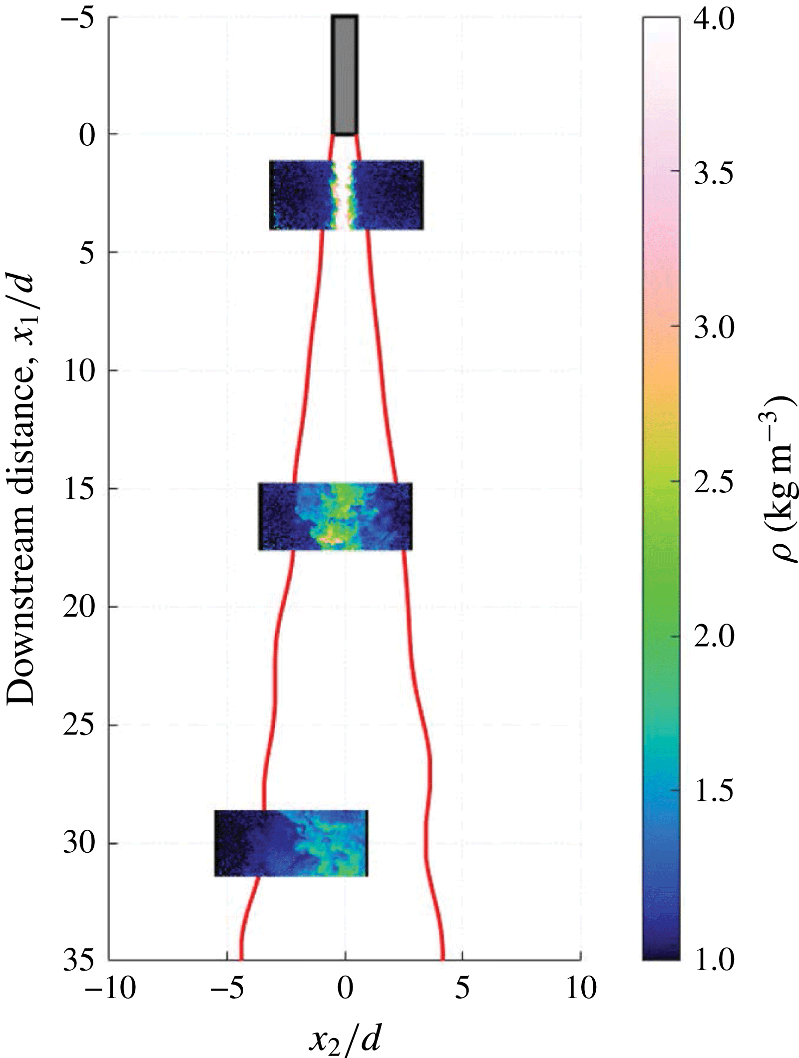
The experimental dataset to be analysed was recently reported in Charonko & Prestridge (Reference Charonko and Prestridge2017). Key characteristics of this dataset are provided below and readers are referred to Charonko & Prestridge (Reference Charonko and Prestridge2017) for more details. A gas jet, a mixture of either air
 $+$
acetone or
 $\text{SF}_{6}+$
acetone, was injected vertically downward from a nozzle into a coflow set up inside a wind tunnel. The two jets were matched by their bulk Reynolds number (
 ${\sim}20\,000$
). For the air jet, the density ratio was 1.2, and that of the
 $\text{SF}_{6}$
jet was 4.2. Simultaneous planar laser-induced fluorescence (PLIF) and two-dimensional two-component particle image velocimetry (2D2C-PIV) measurements were carried out for both jets at three downstream locations,
 $2d$
,
 $16d$
and
 $30d$
, where
 $d=11~\text{mm}$
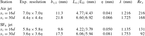
is the nozzle diameter. A definition diagram of the experimental set-up is shown in figure 2 with representative measurement field locations. The computed two-dimensional vector fields are uniformly spaced at 0.287 mm in both directions. Table 2 tabulates the measurement resolution and parameters of the jets at each station.
A schematic diagram of the VD turbulent round jet experiments in Charonko & Prestridge (Reference Charonko and Prestridge2017). Jet diameter
 $d=11~\text{mm}$
.

Experimental conditions. Kolmogorov length scale
 $\unicode[STIX]{x1D702}=(\unicode[STIX]{x1D708}^{3}/\overline{\unicode[STIX]{x1D716}})^{1/4}$
, Taylor microscale
 $\unicode[STIX]{x1D706}=\sqrt{15\unicode[STIX]{x1D708}\overline{u_{1}^{\prime 2}}/\overline{\unicode[STIX]{x1D716}}}$
,
 $\overline{\unicode[STIX]{x1D716}}=$
mean dissipation rate and Taylor Reynolds number
 $Re_{\unicode[STIX]{x1D706}}=\sqrt{\overline{u_{1}^{\prime 2}}}\unicode[STIX]{x1D706}/\unicode[STIX]{x1D708}$
. The dynamic kinematic viscosity
 $\unicode[STIX]{x1D707}$
is
 $1.7\times 10^{-5}~\text{kg}~\text{m}^{-1}~\text{s}^{-1}$
for the air jet and
 $1.55\times 10^{-5}~\text{kg}~\text{m}^{-1}~\text{s}^{-1}$
for the
 $\text{SF}_{6}$
jet. Because the flow is inhomogeneous,
 $\overline{\unicode[STIX]{x1D716}}$
is computed as
 $\overline{\unicode[STIX]{x1D716}}_{\unicode[STIX]{x1D70C}}/\overline{\unicode[STIX]{x1D70C}}_{c}$
, where
 $\overline{\unicode[STIX]{x1D70C}}_{c}\equiv$
local centreline density and
 $\overline{\unicode[STIX]{x1D716}}_{\unicode[STIX]{x1D70C}}=2\unicode[STIX]{x1D707}\{\overline{(\unicode[STIX]{x2202}\text{}\underline{u_{i}^{\prime }}/\unicode[STIX]{x2202}\text{}\underline{x_{k}})(\unicode[STIX]{x2202}\text{}\underline{u_{i}^{\prime }}/\unicode[STIX]{x2202}\text{}\underline{x_{k}})}+\overline{(\unicode[STIX]{x2202}\text{}\underline{\text{}\underline{u_{i}^{\prime }}}/\unicode[STIX]{x2202}\text{}\underline{\text{}\underline{x_{k}}})(\unicode[STIX]{x2202}\text{}\underline{\text{}\underline{u_{i}^{\prime }}}/\unicode[STIX]{x2202}\text{}\underline{\text{}\underline{x_{k}}})}\}$
(see also § 3.3). Similarly,
 $\unicode[STIX]{x1D708}$
is computed by
 $\unicode[STIX]{x1D707}/\overline{\unicode[STIX]{x1D70C}}_{c}$
. Here,
 $L_{11}$
and
 $L_{22}$
represent the Eulerian integral length scale in the (
 $x_{1}$
) streamwise and (
 $x_{2}$
) radial directions;
 $b_{1/2}$
is the jet velocity half-width, defined as the radial position where the Favre-averaged streamwise velocity
 $\tilde{U_{1}}$
is one-half of the jet centreline value.

3.1 Statistical convergence
The third-order velocity structure function
 $\overline{\unicode[STIX]{x1D6FF}u_{i}^{\prime \prime }(\unicode[STIX]{x1D6FF}u_{k}^{\prime \prime })_{\unicode[STIX]{x1D70C}}^{2}}$
(nonlinear interscale transfer term
 $\unicode[STIX]{x1D6F1}$
) normalised by
 $\overline{\unicode[STIX]{x1D70C}_{c}}$
and the Kolmogorov velocity scale
 $u_{Kol}=\sqrt[4]{\unicode[STIX]{x1D708}\overline{\unicode[STIX]{x1D716}}}$
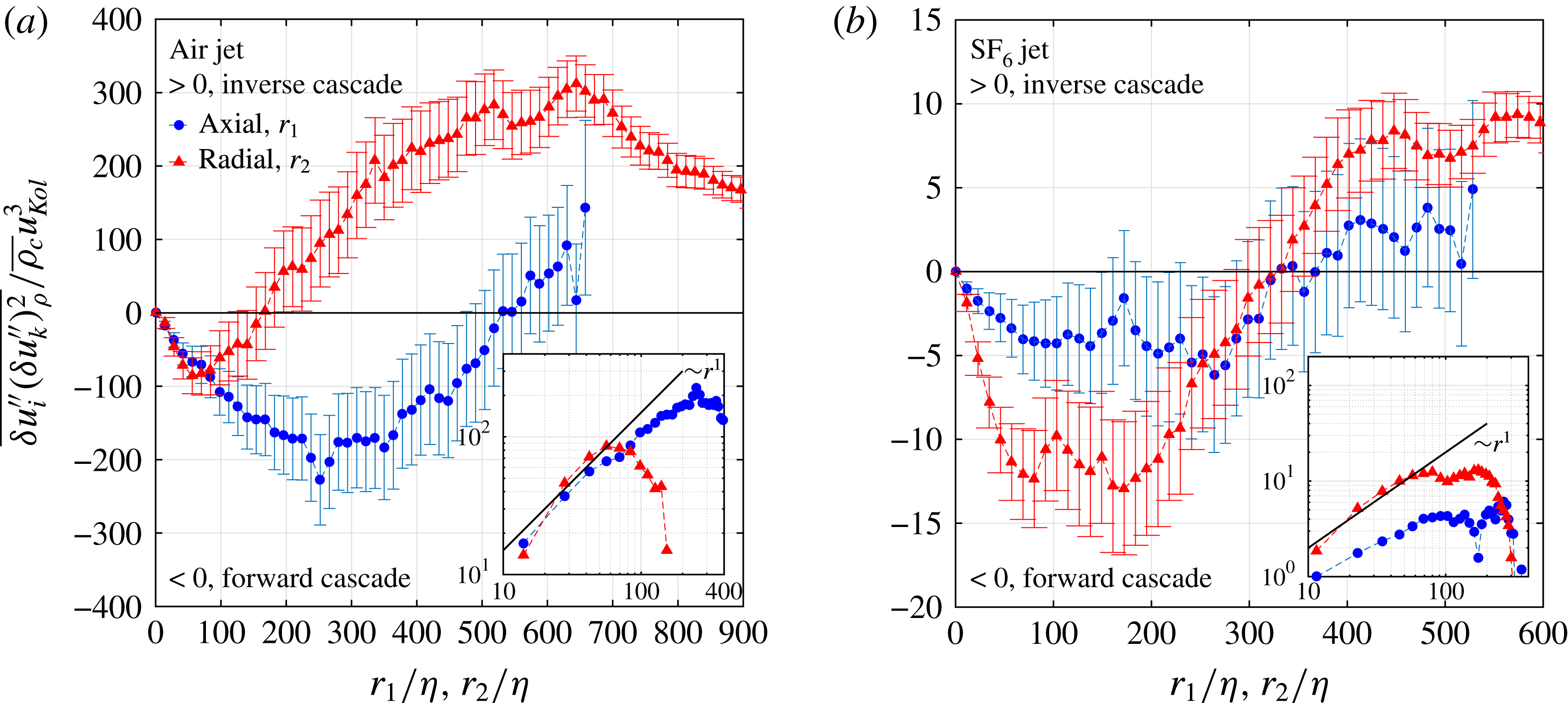
at
 $x_{1}=16d$
in (a) the air jet and (b) the
 $\text{SF}_{6}$
jet. The error bar shown indicates a 95 % confidence interval of
 $\overline{\unicode[STIX]{x1D6FF}u_{i}^{\prime \prime }(\unicode[STIX]{x1D6FF}u_{k}^{\prime \prime })_{\unicode[STIX]{x1D70C}}^{2}}$
. The insets show
 $-\overline{\unicode[STIX]{x1D6FF}u_{i}^{\prime \prime }(\unicode[STIX]{x1D6FF}u_{k}^{\prime \prime })_{\unicode[STIX]{x1D70C}}^{2}}/\overline{\unicode[STIX]{x1D70C}_{c}}u_{Kol}^{3}$
in a log–log plot and highlight the
 $r^{1}$
dependence for scales in the inertial subrange.

The acquisition frequency of the combined PIV/PLIF measurements was 1 Hz, and 10 000 snapshots were taken at each downstream location. Because the longitudinal (downstream) Eulerian integral time scale is of the order of 0.1 s, the data ensemble can be considered as consisting of 10 000 statistically independent samples. Figure 3 shows the third-order structure function
 $\overline{\unicode[STIX]{x1D6FF}u_{i}^{\prime \prime }(\unicode[STIX]{x1D6FF}u_{k}^{\prime \prime })_{\unicode[STIX]{x1D70C}}^{2}}$
versus the separation distances
 $r_{1}$
and
 $r_{2}$
, with error bars constructed from two standard deviations of each data point, giving a 95 % confidence interval for the mean. The standard deviation of
 $\overline{\unicode[STIX]{x1D6FF}u_{i}^{\prime \prime }(\unicode[STIX]{x1D6FF}u_{k}^{\prime \prime })_{\unicode[STIX]{x1D70C}}^{2}}$
is calculated from the square root of the variance of
 $\unicode[STIX]{x1D6FF}u_{i}^{\prime \prime }(\unicode[STIX]{x1D6FF}u_{k}^{\prime \prime })_{\unicode[STIX]{x1D70C}}^{2}$
,
 $$\begin{eqnarray}\displaystyle & \displaystyle \text{Var}(\overline{\unicode[STIX]{x1D6FF}u_{i}^{\prime \prime }(\unicode[STIX]{x1D6FF}u_{k}^{\prime \prime })_{\unicode[STIX]{x1D70C}}^{2}})=\frac{1}{N}[\overline{(\unicode[STIX]{x1D6FF}u_{i}^{\prime \prime }(\unicode[STIX]{x1D6FF}u_{k}^{\prime \prime })_{\unicode[STIX]{x1D70C}}^{2})^{2}}-\overline{\unicode[STIX]{x1D6FF}u_{i}^{\prime \prime }(\unicode[STIX]{x1D6FF}u_{k}^{\prime \prime })_{\unicode[STIX]{x1D70C}}^{2}}^{2}], & \displaystyle\end{eqnarray}$$
where
 $N=10\,000$
is the number of independent samples. The third-order structure function converges to within
 $\pm 30\,\%{-}40\,\%$
of the mean. In figure 3(a), the air jet structure function shows that when
 $r/\unicode[STIX]{x1D702}$
is small,
 $\overline{\unicode[STIX]{x1D6FF}u_{i}^{\prime \prime }(\unicode[STIX]{x1D6FF}u_{k}^{\prime \prime })_{\unicode[STIX]{x1D70C}}^{2}}$
is negative, signifying a forward cascade (2.4). As
 $r/\unicode[STIX]{x1D702}$
increases, the curves in both the axial (
 $r_{1}$
) and radial (
 $r_{2}$
) directions eventually become positive. The zero-crossing point, at larger scales in the axial direction, suggests that the forward cascade persists to larger scales along the jet axis. In the
 $\text{SF}_{6}$
jet, figure 3(b), the normalised magnitudes of the cascade in both directions are much smaller than those in the air jet and the zero-crossing points for the axial and radial directions are both at
 $r/\unicode[STIX]{x1D702}\approx 325$
.
A physical interpretation is that heavy fluids in the
 $\text{SF}_{6}$
jet suppress the energy transfer among scales, and this is most severe along the jet centreline. There are two expected power laws on
 $r$
, namely
 $r^{3}$
for
 $r\sim O(\unicode[STIX]{x1D702})$
and
 $r^{1}$
for
 $r$
within the inertial subrange. The former results from applying a Taylor series expansion to
 $\unicode[STIX]{x1D6FF}u_{i}=u_{i}-u_{i}^{\prime }=-\unicode[STIX]{x1D735}u_{i}\boldsymbol{\cdot }\boldsymbol{r}\sim |\boldsymbol{r}|$
if the small scales are isotropic (this is satisfied to within 15 % in figure 5). Hence,
 $\overline{\unicode[STIX]{x1D6FF}u_{i}^{\prime \prime }(\unicode[STIX]{x1D6FF}u_{k}^{\prime \prime })_{\unicode[STIX]{x1D70C}}^{2}}\sim r^{3}$
, where
 $r=|\boldsymbol{r}|$
. The latter is a consequence of (2.4). Because the smallest resolved scale in the present study is approximately 10
 $\unicode[STIX]{x1D702}$
, only the
 $r^{1}$
power law is captured (see insets).
3.2 Degree of isotropy of fluctuations in velocity, vorticity and scale energy
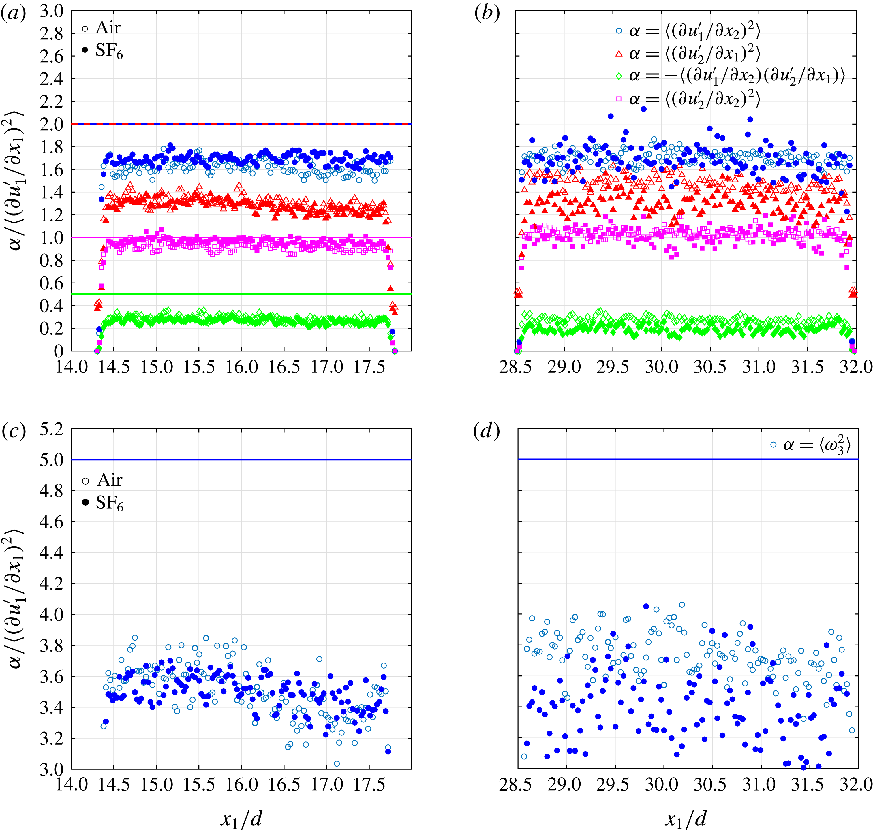
The ratios of the second moments of the velocity derivatives are used to test for local isotropy (Taylor Reference Taylor1935); these isotropic relations are
 $$\begin{eqnarray}\displaystyle & \displaystyle {\displaystyle \frac{\left\langle \left({\displaystyle \frac{\unicode[STIX]{x2202}u_{1}^{\prime }}{\unicode[STIX]{x2202}x_{2}}}\right)^{2}\right\rangle }{\left\langle \left({\displaystyle \frac{\unicode[STIX]{x2202}u_{1}^{\prime }}{\unicode[STIX]{x2202}x_{1}}}\right)^{2}\right\rangle }}={\displaystyle \frac{\left\langle \left({\displaystyle \frac{\unicode[STIX]{x2202}u_{2}^{\prime }}{\unicode[STIX]{x2202}x_{1}}}\right)^{2}\right\rangle }{\left\langle \left({\displaystyle \frac{\unicode[STIX]{x2202}u_{1}^{\prime }}{\unicode[STIX]{x2202}x_{1}}}\right)^{2}\right\rangle }}=2,\quad {\displaystyle \frac{-\left\langle {\displaystyle \frac{\unicode[STIX]{x2202}u_{1}^{\prime }}{\unicode[STIX]{x2202}x_{2}}}{\displaystyle \frac{\unicode[STIX]{x2202}u_{2}^{\prime }}{\unicode[STIX]{x2202}x_{1}}}\right\rangle }{\left\langle \left({\displaystyle \frac{\unicode[STIX]{x2202}u_{1}^{\prime }}{\unicode[STIX]{x2202}x_{1}}}\right)^{2}\right\rangle }}=0.5 & \displaystyle\end{eqnarray}$$
and
 $$\begin{eqnarray}\displaystyle & \displaystyle \frac{\left\langle \left({\displaystyle \frac{\unicode[STIX]{x2202}u_{2}^{\prime }}{\unicode[STIX]{x2202}x_{2}}}\right)^{2}\right\rangle }{\left\langle \left({\displaystyle \frac{\unicode[STIX]{x2202}u_{1}^{\prime }}{\unicode[STIX]{x2202}x_{1}}}\right)^{2}\right\rangle }=1,\quad {\displaystyle \frac{\langle \unicode[STIX]{x1D714}_{3}^{2}\rangle }{\left\langle \left({\displaystyle \frac{\unicode[STIX]{x2202}u_{1}^{\prime }}{\unicode[STIX]{x2202}x_{1}}}\right)^{2}\right\rangle }}=5. & \displaystyle\end{eqnarray}$$
Figure 4 shows how these ratios evolve along the centrelines of the two jets at two different downstream locations. The jets are not isotropic for
 $x_{1}/d\leqslant 30$
, except for the radial moments in both jets, nor are the radial profiles for
 $|x_{2}/b_{1/2}|<1.8$
(not shown). This is in congruence with experimental data by Ganapathisubramani, Lakshminarasimhan & Clemens (Reference Ganapathisubramani, Lakshminarasimhan and Clemens2007). The ratios also become slightly more isotropic at
 $x_{1}/d=30$
.
The variable density of the
 $\text{SF}_{6}$
jet does not appear to affect these ratios, which have values close to their counterparts in the air jet. The mean-square velocity gradients are representative of a range of scales since, for example,
 $\overline{(\unicode[STIX]{x2202}u_{1}^{\prime }/\unicode[STIX]{x2202}x_{1})^{2}}=\int _{0}^{\infty }k_{1}^{2}E_{11}(k_{1})\,\text{d}k_{1}$
, where
 $E_{11}(k_{1})$
is the one-dimensional streamwise spectrum. To assess the level of isotropy at each
 $r$
, the measured distribution of
 $\overline{(\unicode[STIX]{x1D6FF}u_{2}^{\prime \prime })_{\unicode[STIX]{x1D70C}}^{2}}$
is compared with that calculated with the following isotropic relation (Monin & Yaglom Reference Monin and Yaglom1975; Lavoie, Djenidi & Antonia Reference Lavoie, Djenidi and Antonia2007):
 $$\begin{eqnarray}\displaystyle & \displaystyle \overline{(\unicode[STIX]{x1D6FF}u_{2}^{\prime \prime })_{\unicode[STIX]{x1D70C}}^{2}}_{cal}=\frac{r}{2}\frac{\text{d}\overline{(\unicode[STIX]{x1D6FF}u_{1}^{\prime \prime })_{\unicode[STIX]{x1D70C}}^{2}}}{\text{d}r}+\overline{(\unicode[STIX]{x1D6FF}u_{1}^{\prime \prime })_{\unicode[STIX]{x1D70C}}^{2}}, & \displaystyle\end{eqnarray}$$
where the measured distribution of
 $\overline{(\unicode[STIX]{x1D6FF}u_{1}^{\prime \prime })_{\unicode[STIX]{x1D70C}}^{2}}$
is used as the input. The prediction is plotted as the ratio
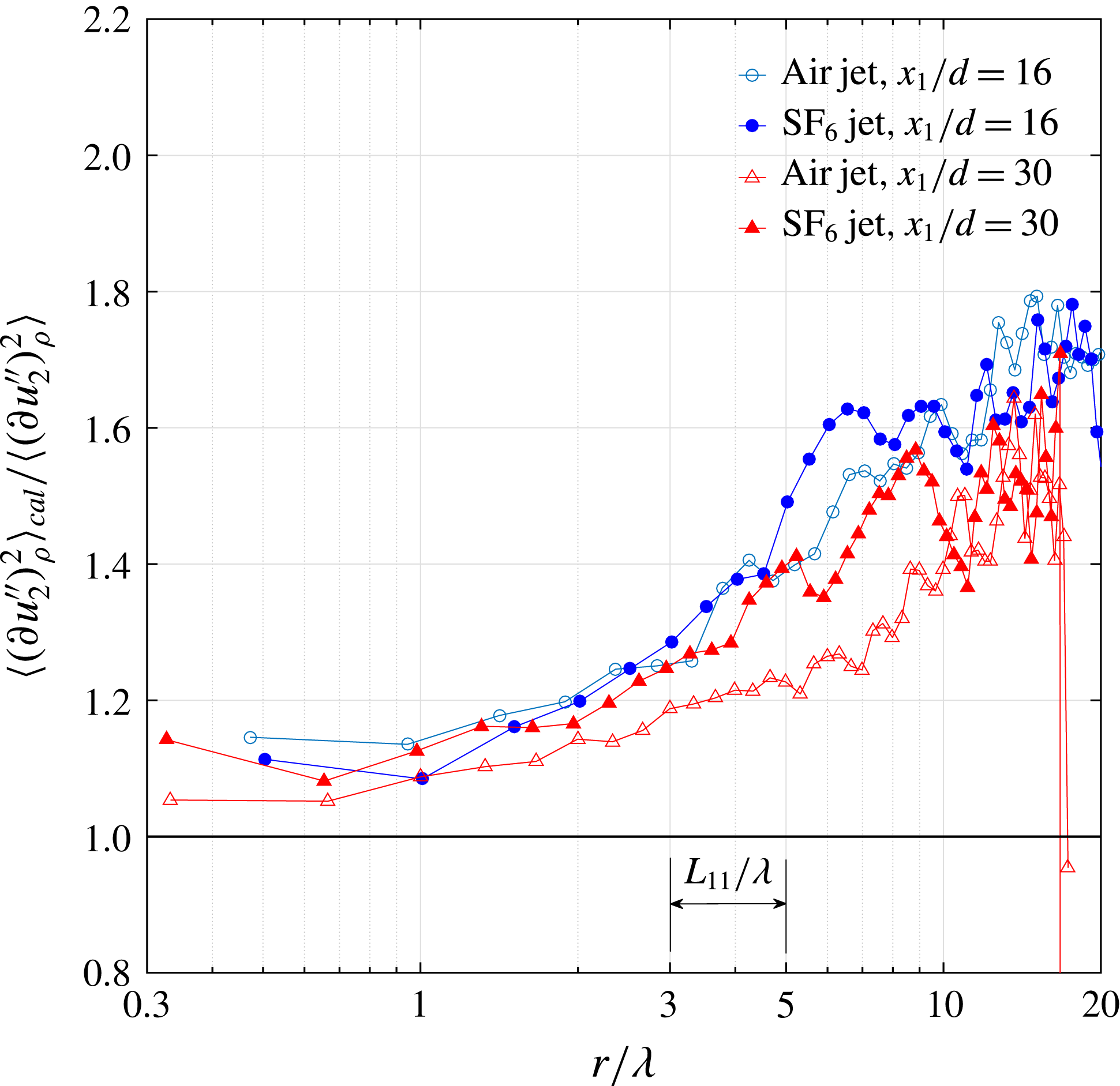
 $\overline{(\unicode[STIX]{x1D6FF}u_{2}^{\prime \prime })_{\unicode[STIX]{x1D70C}}^{2}}_{cal}/\overline{(\unicode[STIX]{x1D6FF}u_{2}^{\prime \prime })_{\unicode[STIX]{x1D70C}}^{2}}$
in figure 5. Figure 5 shows isotropy, satisfied to within 15 % for length scales
 $r/\unicode[STIX]{x1D706}<2$
, in both the air and the
 $\text{SF}_{6}$
jet for the two downstream measurement locations. This is consistent with the structure function calculations of figure 3 because
 $\unicode[STIX]{x1D706}\approx 30\unicode[STIX]{x1D702}$
. As
 $r$
grows, rapid departure from isotropy begins in the range
 $r/\unicode[STIX]{x1D706}\in [3,5]$
, which is also where the streamwise Eulerian length scale
 $L_{11}$
lies. At the largest separations, which are of the same size as
 $b_{1/2}$
, the ratio is between 1.5 and 1.7. This is comparable to the one-point anisotropy ratio
 $\overline{u_{1}^{\prime \prime 2}}/\overline{u_{2}^{\prime \prime 2}}$
(Charonko & Prestridge Reference Charonko and Prestridge2017).
Isotropy improves with
 $x_{1}/d$
for the air jet, while it is impaired by the VD effects in the
 $\text{SF}_{6}$
jet at the same streamwise location. This illustrates the usefulness of the two-point formulation since density effects cannot be unambiguously identified in the ratios of velocity-derivative moments (figure 4).
Streamwise evolution of the ratios of the second moments of the velocity derivatives measured at the jet centrelines for air and
 $\text{SF}_{6}$
at (a,c)
 $x_{1}/d=16$
and (b,d)
 $x_{1}/d=30$
.

Ratio of
 $\overline{(\unicode[STIX]{x1D6FF}u_{2}^{\prime \prime })^{2}}$
calculated using (3.4) to that from experimental data for the air jet (open symbols) and the
 $\text{SF}_{6}$
jet (filled symbols). The isotropic value of the ratio is one and
 $L_{11}$
is the streamwise Eulerian length scale.

3.3 Method of computation of terms in the VD K–H–M equation
To understand scale energy transfer among spherical energy shells of different radii, we transform the experimental data from a Cartesian grid
 $(x_{1},x_{2},x_{3})=(x_{1},x_{2},0)$
to a spherical coordinate system
 $(r,\unicode[STIX]{x1D703},\unicode[STIX]{x1D719})$
. As the dataset is 2D, we effectively have a slice at
 $\unicode[STIX]{x1D719}=0$
that is a polar grid
 $(r,\unicode[STIX]{x1D703})$
. We do not have the full range of all possible orientations of the vector
 $\boldsymbol{r}/r$
, but this is not expected to cause serious issues in the interpretation of results because of jet axisymmetry. Bilinear interpolation is used during the coordinate transformation, in which
 $(r,\unicode[STIX]{x1D703})$
are each partitioned into 80 equidistant points. A convergence study of the interpolation process showed that the transformation results were within
 $\pm 5\,\%$
as long as over 30 points were used, with larger numbers of points reducing the jitter in the interpolation. In the following, the computation of terms in (2.7) is described.
(i)
$\overline{(\unicode[STIX]{x1D6FF}u_{i}^{\prime \prime })_{\unicode[STIX]{x1D70C}}^{2}}=\overline{\unicode[STIX]{x1D6FF}(u_{i}^{\prime \prime })\unicode[STIX]{x1D6FF}(\unicode[STIX]{x1D70C}u_{i}^{\prime \prime })}\approx \overline{\unicode[STIX]{x1D6FF}(u_{1}^{\prime \prime })\unicode[STIX]{x1D6FF}(\unicode[STIX]{x1D70C}u_{1}^{\prime \prime })}+2\overline{\unicode[STIX]{x1D6FF}(u_{2}^{\prime \prime })\unicode[STIX]{x1D6FF}(\unicode[STIX]{x1D70C}u_{2}^{\prime \prime })}$
; the missing out-of-plane velocity structure function
$\overline{\unicode[STIX]{x1D6FF}(u_{3}^{\prime \prime })\unicode[STIX]{x1D6FF}(\unicode[STIX]{x1D70C}u_{3}^{\prime \prime })}$
is approximated by the in-plane radial structure function
$\overline{\unicode[STIX]{x1D6FF}(u_{2}^{\prime \prime })\unicode[STIX]{x1D6FF}(\unicode[STIX]{x1D70C}u_{2}^{\prime \prime })}$
.(ii)
$\unicode[STIX]{x2202}\overline{(\unicode[STIX]{x1D6FF}u_{i}^{\prime \prime })_{\unicode[STIX]{x1D70C}}^{2}}/\unicode[STIX]{x2202}t=0$
since the jet flow is stationary in the Eulerian frame.(iii)
$A=((\text{}\underline{\tilde{U_{k}}}+\text{}\underline{\text{}\underline{\tilde{U_{k}}}})/2)(\unicode[STIX]{x2202}\overline{(\unicode[STIX]{x1D6FF}u_{i}^{\prime \prime })_{\unicode[STIX]{x1D70C}}^{2}}/\unicode[STIX]{x2202}X_{k})\approx ((\text{}\underline{\tilde{U_{1}}}+\text{}\underline{\text{}\underline{\tilde{U_{1}}}})/2)(\unicode[STIX]{x2202}\overline{(\unicode[STIX]{x1D6FF}u_{i}^{\prime \prime })_{\unicode[STIX]{x1D70C}}^{2}}/\unicode[STIX]{x2202}X_{1})$
since the mean flow is flowing predominantly downstream with
$\tilde{U_{2}}\approx \tilde{U_{3}}\approx 0$
, and, therefore, the advection in the radial
$r$
(
$x_{2}$
) and out-of-plane (
$x_{3}$
) directions is negligible in comparison. The streamwise gradient
$\unicode[STIX]{x2202}/\unicode[STIX]{x2202}X_{1}$
is evaluated using a backward difference with spacing of 20 PIV vectors (
${\approx}5.8~\text{mm}=0.5{-}0.6b_{1/2}$
). The results are not sensitive to separations in the range of 10–20 vector spacings.(iv)
$\unicode[STIX]{x1D6F1}=\unicode[STIX]{x2202}\overline{\unicode[STIX]{x1D6FF}u_{k}^{\prime \prime }(\unicode[STIX]{x1D6FF}u_{i}^{\prime \prime })_{\unicode[STIX]{x1D70C}}^{2}}/\unicode[STIX]{x2202}r_{k}\approx (1/r^{2})(\unicode[STIX]{x2202}(r^{2}\overline{\unicode[STIX]{x1D6FF}u_{||}^{\prime \prime }(\unicode[STIX]{x1D6FF}u_{i}^{\prime \prime })_{\unicode[STIX]{x1D70C}}^{2}})/\unicode[STIX]{x2202}r)+(1/r\sin \unicode[STIX]{x1D703})\times (\unicode[STIX]{x2202}\sin \unicode[STIX]{x1D703}\overline{\unicode[STIX]{x1D6FF}u_{\bot }^{\prime \prime }(\unicode[STIX]{x1D6FF}u_{i}^{\prime \prime })_{\unicode[STIX]{x1D70C}}^{2}}/\unicode[STIX]{x2202}\unicode[STIX]{x1D703})$
, following the approach in Valente & Vassilicos (Reference Valente and Vassilicos2015).(v)
$\unicode[STIX]{x1D6F1}_{U}=\unicode[STIX]{x2202}\unicode[STIX]{x1D6FF}\tilde{U_{k}}\overline{(\unicode[STIX]{x1D6FF}u_{i}^{\prime \prime })_{\unicode[STIX]{x1D70C}}^{2}}/\unicode[STIX]{x2202}r_{k}$
is the linear energy flux across
$\boldsymbol{r}$
-space by the differential mean velocity
$\unicode[STIX]{x1D6FF}\tilde{U_{k}}$
, and is evaluated in the same way as
$\unicode[STIX]{x1D6F1}$
.(vi)
$P=-2[\unicode[STIX]{x1D608}_{ik}+\unicode[STIX]{x1D609}_{ik}](\unicode[STIX]{x2202}\unicode[STIX]{x1D6FF}\tilde{U_{i}}/\unicode[STIX]{x2202}r_{k})-[\unicode[STIX]{x1D608}_{ik}-\unicode[STIX]{x1D609}_{ik}](\unicode[STIX]{x2202}\unicode[STIX]{x1D6FF}\tilde{U_{i}}/\unicode[STIX]{x2202}X_{k})$
; the full expression is computed with the available 2D data.(vii)
$T\approx -(1/2)(\unicode[STIX]{x2202}\overline{(\text{}\underline{u_{1}^{\prime \prime }}+\text{}\underline{\text{}\underline{u_{1}^{\prime \prime }}})(\unicode[STIX]{x1D6FF}u_{i}^{\prime \prime })_{\unicode[STIX]{x1D70C}}^{2}}/\unicode[STIX]{x2202}X_{1})-(1/2)(\unicode[STIX]{x2202}\overline{(\text{}\underline{u_{2}^{\prime \prime }}+\text{}\underline{\text{}\underline{u_{2}^{\prime \prime }}})(\unicode[STIX]{x1D6FF}u_{i}^{\prime \prime })_{\unicode[STIX]{x1D70C}}^{2}}/\unicode[STIX]{x2202}X_{2})$
; the streamwise gradient
$\unicode[STIX]{x2202}/\unicode[STIX]{x2202}X_{1}$
is computed in the same manner as the advection term. The radial gradient
$\unicode[STIX]{x2202}/\unicode[STIX]{x2202}X_{2}$
, however, is computed using a spacing of 10 PIV vectors (
${\approx}2.9~\text{mm}=0.26{-}0.3b_{1/2}$
) radially from the jet centreline. A smaller spacing is used because of larger gradients in the radial than the streamwise direction.(viii)
$T_{p}$
is estimated with Lumley’s pressure transport model (Lumley (Reference Lumley1979), see § 5.2).(ix)
$D_{\unicode[STIX]{x1D708}}\approx (2\unicode[STIX]{x1D708}/r^{2})(\unicode[STIX]{x2202}(r^{2}(\unicode[STIX]{x2202}\overline{\unicode[STIX]{x1D6FF}q^{2}}/\unicode[STIX]{x2202}r))/\unicode[STIX]{x2202}r)$
, following the approach in Valente & Vassilicos (Reference Valente and Vassilicos2015). It represents viscous diffusion of energy
$\overline{\unicode[STIX]{x1D6FF}q^{2}}$
across
$\boldsymbol{r}$
-space and is only significant for scales that are of the same order as
$\unicode[STIX]{x1D702}$
.(x)
$D_{\boldsymbol{X},\unicode[STIX]{x1D708}}=(\unicode[STIX]{x1D708}/2)(\unicode[STIX]{x2202}^{2}\overline{\unicode[STIX]{x1D6FF}q^{2}}/\unicode[STIX]{x2202}X_{k}^{2})$
is the
$\overline{\unicode[STIX]{x1D6FF}q^{2}}$
diffusion in physical centroidal space
$\boldsymbol{X}$
and is essentially zero for the present jets, as shown in § 5.2. The second derivative is computed using the standard five-point stencil of the Laplacian.(xi)
$4\overline{\unicode[STIX]{x1D716}}=2\unicode[STIX]{x1D707}\{\overline{(\unicode[STIX]{x2202}\text{}\underline{u_{i}^{\prime }}/\unicode[STIX]{x2202}\text{}\underline{x_{k}})(\unicode[STIX]{x2202}\text{}\underline{u_{i}^{\prime }}/\unicode[STIX]{x2202}\text{}\underline{x_{k}})}+\overline{(\unicode[STIX]{x2202}\text{}\underline{\text{}\underline{u_{i}^{\prime }}}/\unicode[STIX]{x2202}\text{}\underline{\text{}\underline{x_{k}}})\,(\unicode[STIX]{x2202}\text{}\underline{\text{}\underline{u_{i}^{\prime }}}/\unicode[STIX]{x2202}\text{}\underline{\text{}\underline{x_{k}}})}\}$
is directly calculated using the available 2D data with the expression in Tanaka & Eaton (Reference Tanaka and Eaton2007).(xii)
$\unicode[STIX]{x1D707}\unicode[STIX]{x0394}\unicode[STIX]{x1D70C}$
is computed from the available 2D data. This term scales as
$1/Re$
(this follows from the momentum equations) because of
$\unicode[STIX]{x2202}\text{}\underline{\unicode[STIX]{x1D70F}_{ik}^{\prime }}/\unicode[STIX]{x2202}\text{}\underline{x_{k}}$
and
$\unicode[STIX]{x2202}\text{}\underline{\text{}\underline{\unicode[STIX]{x1D70F}_{ik}^{\prime }}}/\unicode[STIX]{x2202}\text{}\underline{\text{}\underline{x_{k}}}$
and is expected to be small. Its maximum magnitude occurs around
$\unicode[STIX]{x1D706}$
and is less than 0.1 % of the dissipation rate
$4\overline{\unicode[STIX]{x1D716}}$
. It is therefore left out in the spherically averaged scale-by-scale energy budget to be discussed in § 5.2.(xiii)
$a_{P}$
is computed with the measured mass flux and the inferred mean pressure gradients from the Favre-averaged mean momentum equations (Charonko & Prestridge Reference Charonko and Prestridge2017).(xiv)
$a_{\unicode[STIX]{x1D70F}}$
is not computed as it is 3–4 orders of magnitude smaller than
$a_{P}$
(Charonko & Prestridge Reference Charonko and Prestridge2017).(xv)
$T_{VD}$
and
$Q$
are computed directly from available 2D data.








Finally, all gradients in
 $\boldsymbol{r}$
-space are computed with the standard second-order central difference. The evolution equation of
 $\overline{(\unicode[STIX]{x1D6FF}u_{i}^{\prime \prime })_{\unicode[STIX]{x1D70C}}^{2}}$
is a function of two spaces,
 $\boldsymbol{X}$
and
 $\boldsymbol{r}$
. To calculate
 $\boldsymbol{X}$
derivatives, as needed in the advection term
 $A$
, by using finite differencing on the discrete experimental data, one needs to evaluate
 $\overline{\unicode[STIX]{x1D6FF}q^{2}}$
at
 $\boldsymbol{X}+\text{d}\boldsymbol{X}$
and subsequently form, for example, the difference
 $\overline{\unicode[STIX]{x1D6FF}q^{2}}(\boldsymbol{r};\boldsymbol{X}+\text{d}\boldsymbol{X})-\overline{\unicode[STIX]{x1D6FF}q^{2}}(\boldsymbol{r};\boldsymbol{X})$
for a forward-Euler approximation of the first derivative at
 $\boldsymbol{X}$
. The overall physical interpretation of the equation should be recognised as the energy balance at a single point
 $\boldsymbol{X}$
under the interactions of a broad spectrum of eddy sizes
 $|\boldsymbol{r}|$
that are oriented in different directions
 $\boldsymbol{r}/|\boldsymbol{r}|$
relative to the origin
 $\boldsymbol{X}$
. In practice, the term ‘broad’ is restricted by the spatial resolution of the experiment or of the numerical simulation. The smallest resolved scale of the jet experiments is approximately 34 %–48 % of the Taylor microscale.
In all subsequent plots,
 $(X_{1},X_{2})=(x_{1},x_{2})=(16d,0)$
, and this corresponds to the midheight of the field of view (FOV) of the combined PLIF/PIV experiments; this choice allowed us to calculate the largest possible range of streamwise separations
 $r_{1}$
from the data. The required two-point correlations are all symmetric differences with respect to this fixed
 $(X_{1},X_{2})$
.
3.4 The appropriateness of the new definition of scale energy,
$\overline{(\unicode[STIX]{x1D6FF}u_{i}^{\prime \prime })_{\unicode[STIX]{x1D70C}}^{2}}$
, for VD flows

The constant- and VD versions of the K–H–M equation both describe the evolution of scale energy. The new definition (2.6) of the scale energy incorporates density as a dynamically significant variable into the original formulation. Its effectiveness in VD flows is demonstrated below using the experimental data.
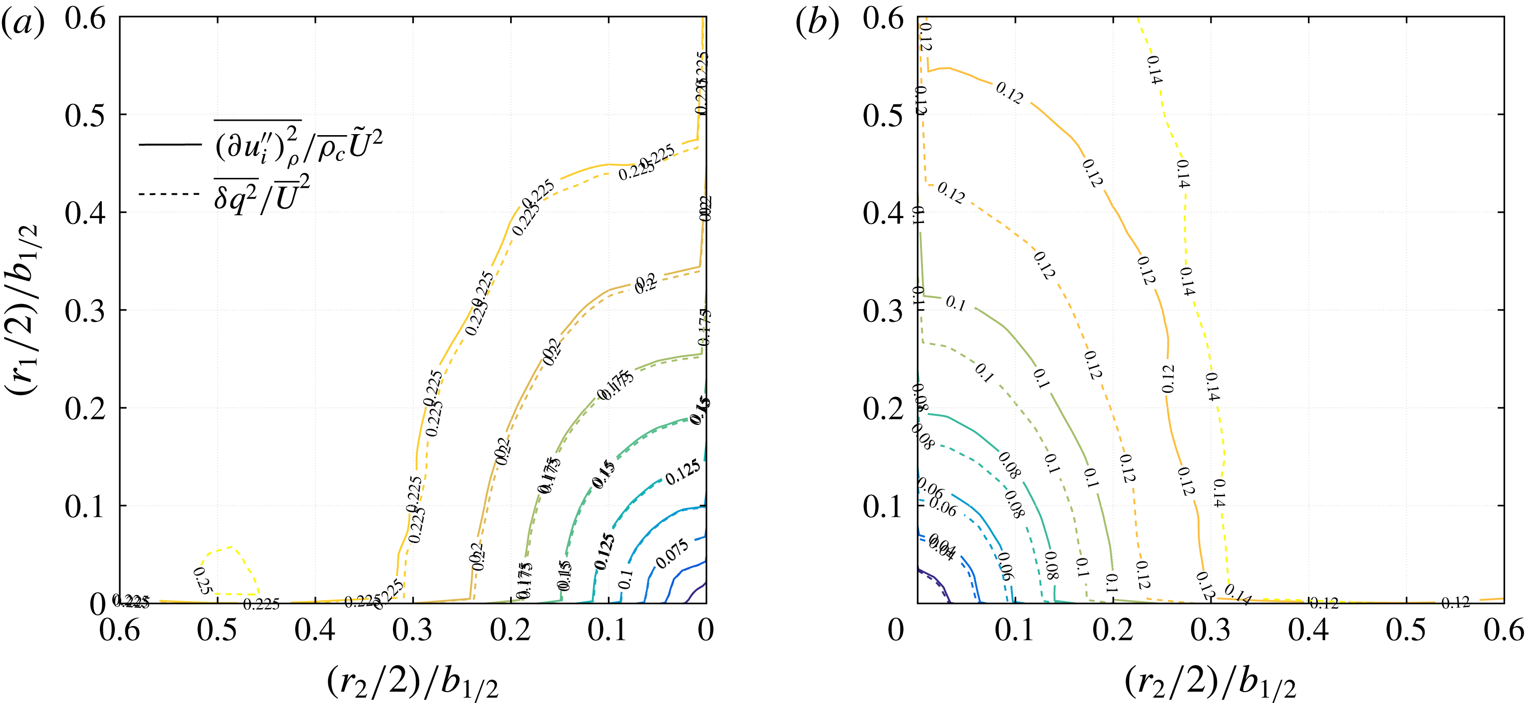
Comparison between the VD (2.6) and single-fluid definitions of scale energy,
 $\overline{(\unicode[STIX]{x1D6FF}u_{i}^{\prime \prime })_{\unicode[STIX]{x1D70C}}^{2}}/\overline{\unicode[STIX]{x1D70C}_{c}}\tilde{U} ^{2}$
(solid lines) and
 $\overline{\unicode[STIX]{x1D6FF}q^{2}}/\overline{U}^{2}$
(dotted lines). The experiments are at
 $x_{1}=16d$
for (a) the air jet and (b) the
 $\text{SF}_{6}$
jet. Here,
 $r_{1}$
and
 $r_{2}$
are the separation distances in the streamwise and radial directions.

The VD and single-fluid definitions for scale energy,
 $\overline{(\unicode[STIX]{x1D6FF}u^{\prime \prime })_{\unicode[STIX]{x1D70C}}^{2}}$
and
 $\overline{\unicode[STIX]{x1D6FF}q^{2}}$
, are shown in figure 6 for both jets at
 $x_{1}=16d$
. The former is normalised by
 $\overline{\unicode[STIX]{x1D70C}}\tilde{U} ^{2}$
(the dimension of
 $\overline{(\unicode[STIX]{x1D6FF}u_{i}^{\prime \prime })_{\unicode[STIX]{x1D70C}}^{2}}$
is
 $([M]/[L^{3}])([L^{2}]/[T^{2}])$
) and the latter by
 $\overline{U}^{2}$
. The separation distances
 $r_{1}$
and
 $r_{2}$
are normalised by the local velocity jet radius
 $b_{1/2}$
. Several observations can be made. First, the two definitions yield essentially the same set of isocontours for the air jet, whereas they give drastically different results for the
 $\text{SF}_{6}$
jet. The equality of the two sets of contours gives
 $\overline{(\unicode[STIX]{x1D6FF}u_{i}^{\prime \prime })_{\unicode[STIX]{x1D70C}}^{2}}=\overline{\unicode[STIX]{x1D70C}}\overline{\unicode[STIX]{x1D6FF}q^{2}}$
(note that
 $\tilde{U} \approx \overline{U}\gg \text{mass flux}~a_{i}=\overline{\unicode[STIX]{x1D70C}u_{i}^{\prime }}/\overline{\unicode[STIX]{x1D70C}}$
), meaning that the density is not dynamically relevant and can be treated as constant. The local Atwood number
 $At=(s-1)/(s+1)$
based on the centreline density, where
 $s$
is the density ratio, is 0.043 for the air jet and 0.33 for the
 $\text{SF}_{6}$
jet. The air jet result is consistent with the commonly accepted upper limit (
 $=0.05$
) of
 $At$
for Boussinesq flows (Livescu et al.
Reference Livescu, Ristorcelli, Peterson and Gore2010). On the other hand, the difference in the contours in the
 $\text{SF}_{6}$
jet reflects the non-Boussinesq character of the heavy jet and supports the use of
 $\overline{(\unicode[STIX]{x1D6FF}u^{\prime \prime })_{\unicode[STIX]{x1D70C}}^{2}}$
to capture VD effects.
Second, in the heavy jet, the agreement between the two sets of contours improves when
 $r_{1}$
and
 $r_{2}$
decrease. This indicates that the small scales are relatively immune to VD effects in the jet and provides empirical evidence supporting the discussions of (2.9). In the absence of strong density discontinuities, such as shock fronts, the dissipation mechanism of fluid energy in VD flows is akin to that in constant-density flows.
Third, regardless of their definitions, the tendency of small scales towards isotropy is evident because as
 $r_{1}$
and
 $r_{2}$
decrease, the contours progressively become more circular. However, as we have seen in figures 4 and 5, the approach to local isotropy is neither complete nor perfect. The above discussion demonstrates the appropriateness of our new definition of scale energy (2.6) in VD flows. In the ensuing sections, terms in the VD K–H–M equation (2.7) are analysed.
4 Scale-by-scale energy transfer
4.1 Directionally dependent interscale transfer
As discussed in § 2, the strength of the two-point K–H–M equation is the appearance of the interscale energy transfer terms,
 $\unicode[STIX]{x1D6F1}_{U}$
and
 $\unicode[STIX]{x1D6F1}$
, with their sum giving the total energy transfer rate across the scale
 $r$
. Mathematically, these terms are the divergences of the vector fields,
 $\unicode[STIX]{x1D6FF}\tilde{U} _{k}\overline{(\unicode[STIX]{x1D6FF}u_{i}^{\prime \prime })_{\unicode[STIX]{x1D70C}}^{2}}$
and
 $\overline{\unicode[STIX]{x1D6FF}u_{k}^{\prime \prime }(\unicode[STIX]{x1D6FF}u_{i}^{\prime \prime })_{\unicode[STIX]{x1D70C}}^{2}}$
, in the
 $\boldsymbol{r}$
-space. Since a negative/positive divergence indicates a converging/diverging vector field, the direction of energy flux is thus from large/small to small/large scales. First, we look at the linear term at
 $x_{1}=16d$
of both jets in figure 7;
 $\unicode[STIX]{x1D6F1}_{U}$
is normalised by the jet centreline variable
 $\overline{\unicode[STIX]{x1D70C}_{c}}(\tilde{U_{c}}^{3}/b_{1/2})$
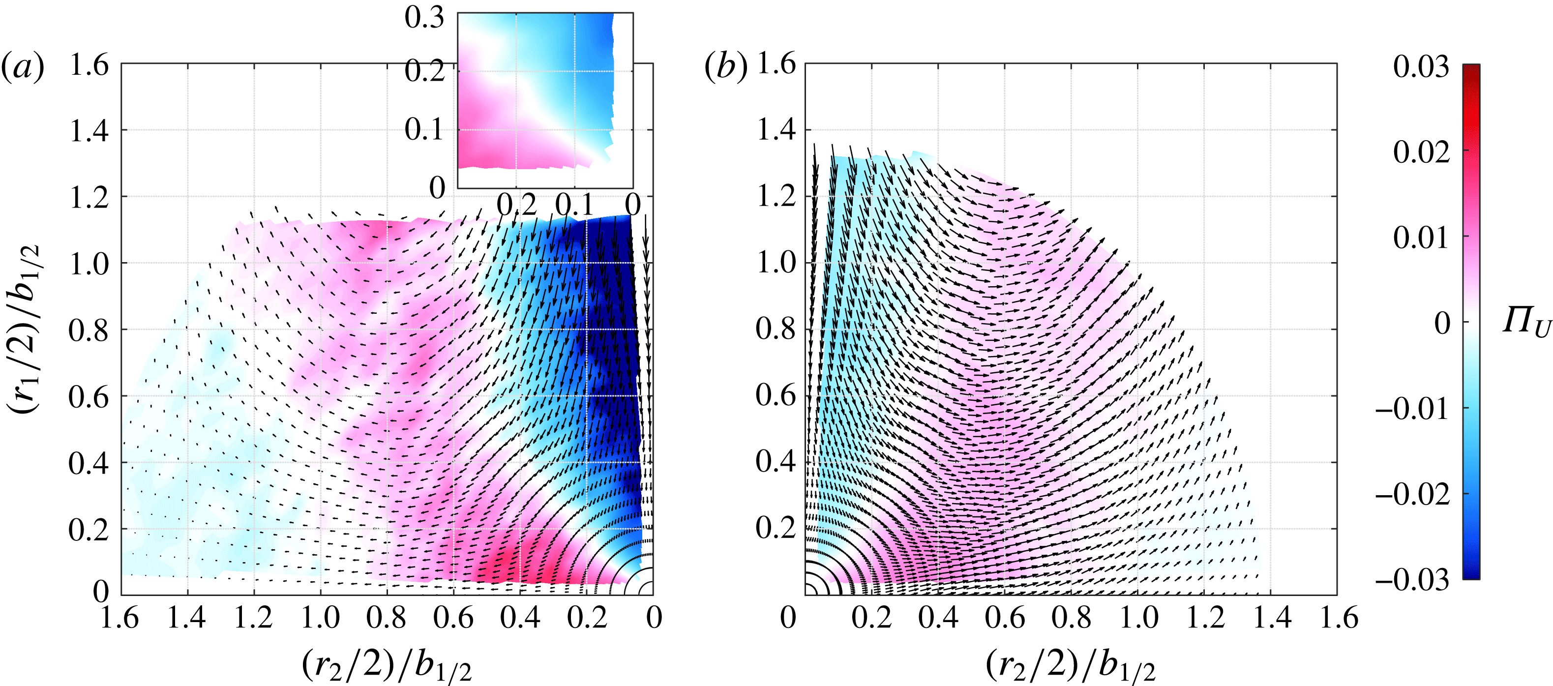
. Regions of blue indicate
 $\unicode[STIX]{x1D6F1}_{U}<0$
, a forward energy transfer, and regions of red indicate
 $\unicode[STIX]{x1D6F1}_{U}>0$
, an inverse energy transfer, with the transition
 $\unicode[STIX]{x1D6F1}_{U}\approx 0$
in white. The corresponding vector field of
 $\unicode[STIX]{x1D6F1}_{U}$
,
 $\unicode[STIX]{x1D6FF}\tilde{U} _{k}\overline{(\unicode[STIX]{x1D6FF}u_{i}^{\prime \prime })_{\unicode[STIX]{x1D70C}}^{2}}$
, indicates a forward transfer when the vectors point towards the origin. The separation distances are divided by two and then normalised by
 $b_{1/2}$
; the division by two reflects the symmetric difference with respect to the jet centreline from which terms like
 $\unicode[STIX]{x1D6FF}\tilde{U} _{k}$
are calculated.
Linear interscale energy transfer
 $\unicode[STIX]{x1D6F1}_{U}=(\unicode[STIX]{x2202}\unicode[STIX]{x1D6FF}\tilde{U_{k}}\overline{(\unicode[STIX]{x1D6FF}u_{i}^{\prime \prime })_{\unicode[STIX]{x1D70C}}^{2}})/\unicode[STIX]{x2202}r_{k}$
in (a) the air jet and (b) the
 $\text{SF}_{6}$
jet at
 $x_{1}=16d$
. The vector field,
 $\unicode[STIX]{x1D6FF}\tilde{U_{k}}\overline{(\unicode[STIX]{x1D6FF}u_{i}^{\prime \prime })_{\unicode[STIX]{x1D70C}}^{2}}$
, is overlaid on the
 $\unicode[STIX]{x1D6F1}_{U}$
colour map. The inset in (a) shows a close-up of
 $\unicode[STIX]{x1D6F1}_{U}$
of the air jet near the origin.

The air jet interscale energy transfer shown in figure 7(a) shows a strong forward transfer in the jet axial direction, as indicated by the dark blue. The axial forward energy transfer in the air jet is over the entire range of scales measured and is a result of the decay of the mean centreline jet velocity.
The sign change of
 $\unicode[STIX]{x1D6F1}_{U}$
along approximately the
 $45^{\circ }$
line for the air jet reflects the inhomogeneity of the flow due to a sign change in the mean entrainment (radial) velocity at that location (Lee & Chu Reference Lee and Chu2003). In spatially homogeneous flows, e.g. grid turbulence (Gomes-Fernandes et al.
Reference Gomes-Fernandes, Ganapathisubramani and Vassilicos2015), there is no differential in the mean flow, so
 $\unicode[STIX]{x1D6F1}_{U}$
is zero.
The situation is slightly different for the heavy
 $\text{SF}_{6}$
jet in figure 7(b). A wide range of off-axis eddies exhibiting an inverse transfer (red region) penetrates down to the smallest resolved scales (
 ${\approx}12\unicode[STIX]{x1D702}$
) in the experiment. Signatures of the mean jet centreline and radial entrainment velocities, as discussed for the air jet, can still be seen in the axially and radially aligned eddies, but these are confined to a narrower region close to the centreline.
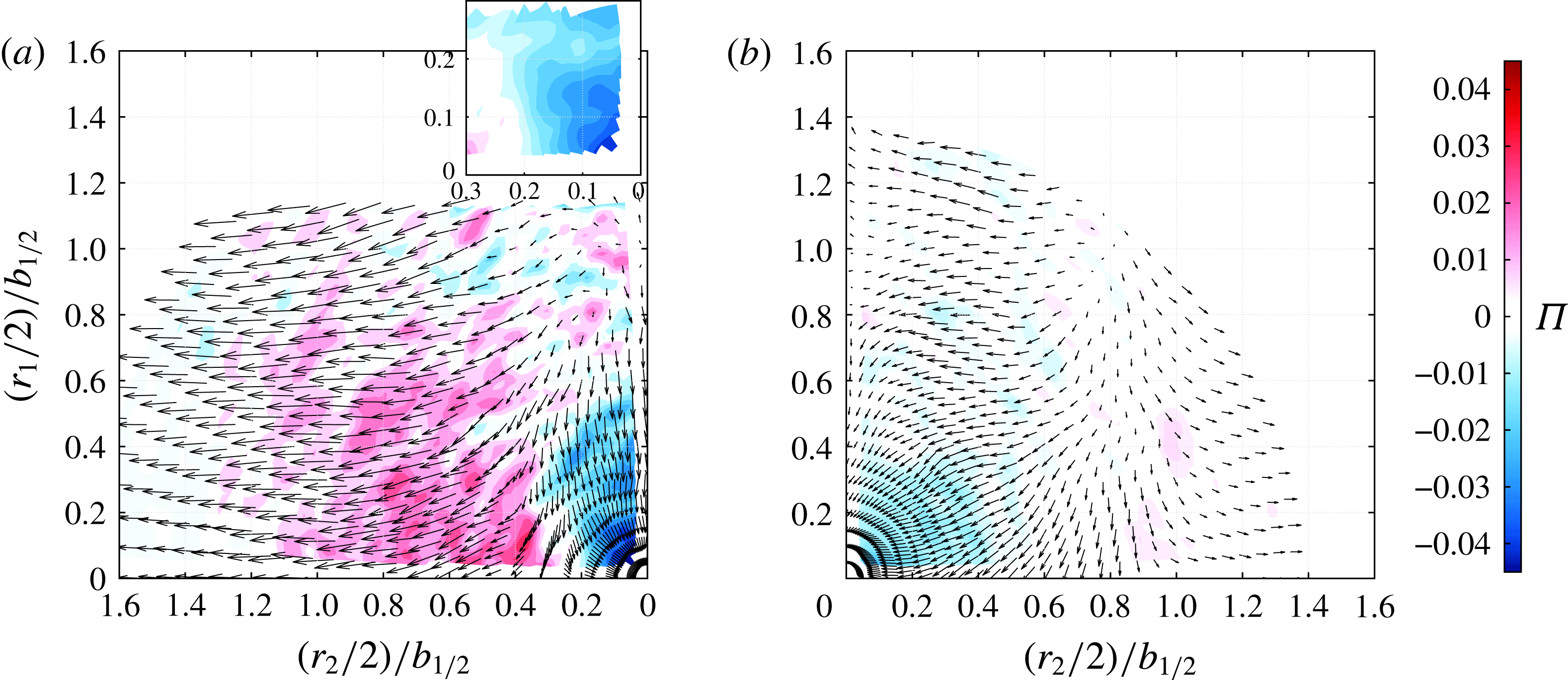
Nonlinear interscale energy transfer
 $\unicode[STIX]{x1D6F1}=(\unicode[STIX]{x2202}\overline{\unicode[STIX]{x1D6FF}u_{k}^{\prime \prime }(\unicode[STIX]{x1D6FF}u_{i}^{\prime \prime })_{\unicode[STIX]{x1D70C}}^{2}})/\unicode[STIX]{x2202}r_{k}$
in (a) the air jet and (b) the
 $\text{SF}_{6}$
jet at
 $x_{1}=16d$
. The vector field,
 $\overline{\unicode[STIX]{x1D6FF}u_{k}^{\prime \prime }(\unicode[STIX]{x1D6FF}u_{i}^{\prime \prime })_{\unicode[STIX]{x1D70C}}^{2}}$
, is overlaid on the
 $\unicode[STIX]{x1D6F1}$
colour map. The inset in (a) shows a close-up of
 $\unicode[STIX]{x1D6F1}$
of the air jet near the origin; the contours are more circular than those of
 $\unicode[STIX]{x1D6F1}_{U}$
in figure 7(a), indicating that the nonlinear transfer is more isotropic than the linear transfer.

The term
 $\unicode[STIX]{x1D6F1}$
is the nonlinear mechanism responsible for the transfer of kinetic energy among turbulent length scales. The traditional energy cascade is nominally independent of the inhomogeneous large scales insofar as they only set the dissipation rate. The term
 $\unicode[STIX]{x1D6F1}$
is therefore amendable to turbulence modelling in that it has the potential of being universal across different flows. To date, it is not known how VD changes
 $\unicode[STIX]{x1D6F1}$
; a particularly interesting question is whether VD effects will change the scale-invariance property of the energy cascade. We explore the answer to this question below.
Figure 8 shows the normalised nonlinear transfer
 $\unicode[STIX]{x1D6F1}$
term, and a forward cascade is present in both jets. The air jet in figure 8(a) shows a forward cascade in the axial direction at the small scales, and the magnitudes of the linear and nonlinear transfer terms in the air jet are similar (compare figures 7
a and 8
a). A closer look at the isocontours near the origin reveals that
 $\unicode[STIX]{x1D6F1}$
is more isotropic than
 $\unicode[STIX]{x1D6F1}_{U}$
, agreeing with observations in figures 5 and 6. The nonlinear term shows a strong inverse cascade among radially aligned eddies larger than
 $r_{2}/2>0.3b_{1/2}$
, a length scale greater than
 $L_{11}$
.
The
 $\text{SF}_{6}$
jet in figure 8(b) has a forward cascade at small scales. A notable difference is seen in the radial eddies, for which the forward cascade extends to larger scales than in the air jet (
 $r_{2}/2=0.6b_{1/2}$
versus
 $0.3b_{1/2}$
). A possible reason for the greater extent of the forward cascade is that heavy fluid in the
 $\text{SF}_{6}$
jet mixes more slowly with the surrounding lighter fluid than in the Boussinesq air jet (Livescu et al.
Reference Livescu, Ristorcelli, Peterson and Gore2010), so that the velocities of the heavy fluid decorrelate less rapidly. This supports a more persistent forward cascade over a larger range of scales. The linear and nonlinear transfer terms behave similarly further downstream at
 $x_{1}=30d$
(not shown).
4.2 Directionally independent interscale transfer
Comparison between the measured third-order velocity structure function
 $\overline{\unicode[STIX]{x1D6FF}\boldsymbol{u}_{||}(\unicode[STIX]{x1D6FF}u_{i}^{\prime \prime })_{\unicode[STIX]{x1D70C}}^{2}}$
and the prediction by (2.4) in the inertial subrange. (a) Present data with air jet data shown as open symbols and
 $\text{SF}_{6}$
jet data shown as filled symbols. (b) Comparison with round jet data (
 $\times$
) in Burattini et al. (Reference Burattini, Antonia and Danaila2005), 2D wake data (♢) in Thiesset et al. (Reference Thiesset, Antonia and Danaila2013), grid turbulence data (
 $\star$
) in Zhou & Antonia (Reference Zhou and Antonia2000), (▹) in Gagne et al. (Reference Gagne, Castaing, Baudet and Malecot2004) and (▫) in Van de Water & Herweijer (Reference Van de Water and Herweijer1999), and forced turbulence data (◂) in Fukayama et al. (Reference Fukayama, Oyamada, Nakano, Gotoh and Yamamoto2000), (▾) in Gotoh, Fukayama & Nakano (Reference Gotoh, Fukayama and Nakano2002) and (▪) in Moisy, Tabeling & Willaime (Reference Moisy, Tabeling and Willaime1999), together with model predictions (——) by Aivalis et al. (Reference Aivalis, Sreenivasan, Tsuji, Klewicki and Biltoft2002). For the decaying grid turbulence and forced turbulence datasets, a constant factor of
 $5/3$
is multiplied to the reported data to account for the difference between the
 $4/5$
-law and the
 $4/3$
-law (2.4). The inset in (b) shows the same data points in a linear–linear space to emphasise their behaviour in their range of
 $Re_{\unicode[STIX]{x1D706}}$
.

The scale-space plot of
 $\unicode[STIX]{x1D6F1}$
contains both magnitude and directional information. In building turbulence models, the interest is often in specifying the interscale flux across a scale
 $r$
independent of its orientations. We therefore examine the orientation-independent nonlinear energy flux below using (2.4). The experimental values are calculated by spherically averaging the vector fields in figure 8 (denoted by
 $(\cdot )^{a}$
; see the next section). The resulting spherically averaged energy transfer is then a sole function of eddy size
 $r=|\boldsymbol{r}|$
. The curves are then plotted as
 $-\overline{\unicode[STIX]{x1D6FF}\boldsymbol{u}_{||}(\unicode[STIX]{x1D6FF}u_{i}^{\prime \prime })_{\unicode[STIX]{x1D70C}}^{2}}^{a}/\overline{\unicode[STIX]{x1D716}}^{a}r$
against
 $r/b_{1/2}$
in figure 9(a), where the abscissa has been normalised by the velocity half-width
 $b_{1/2}$
to remove the effect of jet growth. Because the raw dissipation rates contain experimental uncertainties, the dissipation rate used in the above normalisation is obtained from a consideration of satisfying the spherically averaged scale-by-scale energy budget (5.2). This is necessary for a meaningful comparison between the present data and other published datasets. More details of this procedure are given in § 5.2.
The Kolmogorov
 $4/5$
-law, or its equivalent form, (2.4), is obtained from the relation
 $\unicode[STIX]{x1D6F1}=-4\overline{\unicode[STIX]{x1D716}}$
(2.3) after integration over a sphere of radius
 $r$
and assuming local isotropy. In the inertial subrange, this yields the equation
 $\overline{\unicode[STIX]{x1D6FF}\boldsymbol{u}_{||}(\unicode[STIX]{x1D6FF}u_{i}^{\prime \prime })_{\unicode[STIX]{x1D70C}}^{2}}=-(4/3)\overline{\unicode[STIX]{x1D716}}r$
which states a scale-invariant energy cascade since the scale-normalised energy transfer rate,
 $-\overline{\unicode[STIX]{x1D6FF}\boldsymbol{u}_{||}(\unicode[STIX]{x1D6FF}u_{i}^{\prime \prime })_{\unicode[STIX]{x1D70C}}^{2}}/\overline{\unicode[STIX]{x1D716}}r=4/3$
, is a constant. Strictly speaking, this asymptotic 4/3-state is asserted by Kolmogorov to exist in stationary turbulence (Kolmogorov Reference Kolmogorov1941) when the Reynolds number is sufficiently large and when the local equilibrium hypothesis holds. Whether such a Kolmogorov equilibrium state exists in non-stationary turbulence remains an open question. Even if the equilibrium state does exist, the largest-
 $Re_{\unicode[STIX]{x1D706}}$
experiments achieved
 $O(10^{3})$
(Warhaft Reference Warhaft2009) insinuate that a high Reynolds number is necessary, but possibly not sufficient, for attaining equilibrium in non-stationary turbulence. Below, we discuss the variation of scale-normalised energy flux with
 $Re_{\unicode[STIX]{x1D706}}$
for our experiments, comparing them with other types of equilibrium and non-equilibrium flows.
Figure 9(a) shows that the present experiments do not meet the Kolmogorov 4/3 prediction for stationary turbulence. There is a range of scales
 $0.1{-}0.3b_{1/2}$
for which
 $-\overline{\unicode[STIX]{x1D6FF}\boldsymbol{u}_{||}(\unicode[STIX]{x1D6FF}u_{i}^{\prime \prime })_{\unicode[STIX]{x1D70C}}^{2}}^{a}/\overline{\unicode[STIX]{x1D716}}^{a}r$
peaks, but at a value lower than 4/3. For example, the air and
 $\text{SF}_{6}$
jets at
 $x_{1}=16d$
, having
 $Re_{\unicode[STIX]{x1D706}}=216$
and 131, have a value of approximately 1.05. So, for both jets, the higher
 $Re_{\unicode[STIX]{x1D706}}$
are associated with higher transfer rates. The high values of the transfer rates in the heavy jet are related to the strong inverse energy transfer in the linear interscale energy flux term seen in figure 7(b) and will be discussed in detail in § 5.4.
To compare the deviations from the Kolmogorov equilibrium state as a function of
 $Re_{\unicode[STIX]{x1D706}}$
between the present jets and other types of flows, we plot the maximum scale-normalised energy transfer
 $|-\overline{\unicode[STIX]{x1D6FF}\boldsymbol{u}_{||}(\unicode[STIX]{x1D6FF}u_{i}^{\prime \prime })_{\unicode[STIX]{x1D70C}}^{2}}^{a}/\overline{\unicode[STIX]{x1D716}}^{a}r|_{max}$
in figure 9(b) for (i) a round jet measured at
 $x_{1}/d=40$
, (ii) wakes behind 2D bluff bodies of different geometries, (iii) decaying grid turbulence and (iv) forced, stationary and isotropic turbulence in a periodic box. A model prediction of the variation of maximum energy transfer with
 $Re_{\unicode[STIX]{x1D706}}$
is also included; the predictions are based on a model for the second-order velocity structure function (Aivalis et al.
Reference Aivalis, Sreenivasan, Tsuji, Klewicki and Biltoft2002), and it approaches the asymptotic 4/3 value for
 $Re_{\unicode[STIX]{x1D706}}\sim 10^{5}$
(Antonia & Burattini Reference Antonia and Burattini2006).
The four types of flow listed in the previous paragraph have different trajectories towards the theoretical 4/3 asymptote. The forced turbulence has the fastest trajectory because the turbulence is designed to satisfy Kolmogorov’s postulates. The air jet data points and of Burattini et al. (Reference Burattini, Antonia and Danaila2005) are close to the predictions of the Aivalis model. Because the model, and its variants, contains parameters that can be tuned to match a particular flow type (Antonia & Burattini Reference Antonia and Burattini2006), the reasonably good agreement between its predictions and the jet data suggests that the trend of the jet is consistent, at least with respect to
 $Re_{\unicode[STIX]{x1D706}}$
. Decaying flows (jets, wakes and grid turbulence) that have the same
 $Re_{\unicode[STIX]{x1D706}}$
have large variations in the measured maximum scale-normalised energy transfer rate; see, for example, the range
 $Re_{\unicode[STIX]{x1D706}}=100{-}400$
. This means that universality of turbulence at scales of the order of
 $\unicode[STIX]{x1D706}$
(where
 $|-\overline{\unicode[STIX]{x1D6FF}\boldsymbol{u}_{||}(\unicode[STIX]{x1D6FF}u_{i}^{\prime \prime })_{\unicode[STIX]{x1D70C}}^{2}}^{a}/\overline{\unicode[STIX]{x1D716}}^{a}r|_{max}$
occurs) is non-existent at these moderate values of
 $Re_{\unicode[STIX]{x1D706}}$
as it depends on the flow type. The
 $\text{SF}_{6}$
jet data points lie in the same range as the forced turbulence datasets. This occurs because the dense jet turbulence is more ‘stationary’ with respect to downstream distances
 $x_{1}$
than the Boussinesq air jet; in the range
 $x_{1}=16d{-}30d$
, the t.k.e. of the dense jet decayed by only 20 % whereas the air jet experienced a 44 % reduction (see figure 13 of Charonko & Prestridge (Reference Charonko and Prestridge2017)). Hence, the dense jet is closer to stationary turbulence than the air jet. We defer a detailed physical explanation of this peculiar behaviour to § 5.4 after examining the scale-by-scale energy budget of the jet in § 5.2. It may not be possible to develop a generalised model for the dependence of the energy flux on
 $Re_{\unicode[STIX]{x1D706}}$
for turbulent flows, especially when VD effects are present.
5 Scale-by-scale energy budget
5.1 Spatial variation of dissipation, production, advection and transport of scale energy
The analysis of one-point t.k.e. budgets by Charonko & Prestridge (Reference Charonko and Prestridge2017) reveals several key differences at the centreline between the air and
 $\text{SF}_{6}$
jets. These include (i) negative production, (ii) positive transport and (iii) lower advection. These observations are further interpreted here using the spatial variation in scale space of the remaining terms appearing in the VD K–H–M equation.
Distributions of the dissipation rate (a,b) and production (c,d) of scale energy
 $\overline{(\unicode[STIX]{x1D6FF}u_{i}^{\prime \prime })_{\unicode[STIX]{x1D70C}}^{2}}$
in (
 $r_{1},r_{2}$
)-space for (a,c) the air jet and (b,d) the
 $\text{SF}_{6}$
jet at
 $x_{1}=16d$
.

Distributions of the transport (a,b) and advection (c,d) of scale energy
 $\overline{(\unicode[STIX]{x1D6FF}u_{i}^{\prime \prime })_{\unicode[STIX]{x1D70C}}^{2}}$
in (
 $r_{1},r_{2}$
)-space for (a,c) the air jet and (b,d) the
 $\text{SF}_{6}$
jet at
 $x_{1}=16d$
. The insets show a line profile of the distribution along the dotted line for comparison.

The spatial distributions in
 $(r_{1},r_{2})$
-space of
 $4\overline{\unicode[STIX]{x1D716}}$
and
 $P$
are shown for both jets at
 $x_{1}=16d$
in figure 10. The plotted dissipation is normalised by the value at the origin,
 $4\overline{\unicode[STIX]{x1D716}(0,0)}$
, while
 $P$
is normalised by the local dissipation
 $4\overline{\unicode[STIX]{x1D716}}$
. Figure 10(a,b) shows that the dissipation varies by less than 20 % for
 $(r_{2}/2)<0.8b_{1/2}$
in both jets, and this region extends to
 $0.9b_{1/2}$
for the
 $\text{SF}_{6}$
jet. The dissipation
 $4\overline{\unicode[STIX]{x1D716}}$
is approximately constant along the streamwise direction
 $r_{1}$
, whereas radial gradients are large. The spatial variation of production relative to dissipation (figure 10
c,d) is similar in both jets;
 $P/(4\overline{\unicode[STIX]{x1D716}})$
is low along the jet axis (
 $r_{2}/2<0.2b_{1/2}$
) and reaches its maximum at the shear layer (
 $r_{2}/2=0.8b_{1/2}$
). The peak location can be compared with that of the production term in the t.k.e. budget equation (see figure 15(a) in Charonko & Prestridge (Reference Charonko and Prestridge2017)). Further,
 $P$
is positive at the origin for the
 $\text{SF}_{6}$
jet, even though the production term in the one-point t.k.e. budget was negative. This apparent contradiction is resolved by recognising that two-point correlations only reduce to their one-point counterparts when
 $r$
becomes larger than the correlation length scale (Marati et al.
Reference Marati, Casciola and Piva2004), e.g.
 $L_{11}\approx 0.4b_{1/2}$
from table 2. The observation that
 $P>0$
for all measured scales here means that the negative production (in the sense of the one-point t.k.e. budget) is a localised phenomenon because it is confined to a range of scales smaller than
 $L_{11}$
.
Positive transport and lower advection in the
 $\text{SF}_{6}$
jet were observed in the single-point analyses, and figure 11 shows the comparison for the normalised transport term
 $T/(4\overline{\unicode[STIX]{x1D716}})$
and the advection term
 $-A/(4\overline{\unicode[STIX]{x1D716}})$
. The insets in the
 $T/(4\overline{\unicode[STIX]{x1D716}})$
plots (a,b) show a line profile of the quantity as a function of the radial separation
 $r_{2}$
along the dotted line. These line profiles resemble the corresponding term in the single-point t.k.e. equation when
 $r_{2}$
is greater than the flow integral length scale (Marati et al.
Reference Marati, Casciola and Piva2004). In both jets,
 $T/(4\overline{\unicode[STIX]{x1D716}})$
crosses zero at approximately
 $(r_{2}/2)/b_{1/2}=x_{2}/b_{1/2}\approx 1.2$
and becomes positive thereafter (see figure 15(a) in Charonko & Prestridge (Reference Charonko and Prestridge2017)). However, notable differences are seen in the spatial distribution of the transport term. While
 $T/(4\overline{\unicode[STIX]{x1D716}})$
is negative over all measured
 $r_{1}$
separations in the air jet, it is positive in the
 $\text{SF}_{6}$
jet, indicating that axially aligned eddies are gaining energy from neighbouring streamwise spatial points. Such transfer is very non-local when compared with the two-point production
 $P$
. This is consistent with the single-point t.k.e. budget of the
 $\text{SF}_{6}$
jet, where the turbulent transport term was measured positive at the jet centreline (Charonko & Prestridge Reference Charonko and Prestridge2017).
Regarding the distribution of the advection term,
 $-A/(4\overline{\unicode[STIX]{x1D716}})$
in the
 $\text{SF}_{6}$
jet is less organised and has smaller magnitudes than in the air jet, probably reflecting the influence of VD effects, and consistent with the lower advection observed in the single-point analysis.
5.2 Spherically averaged scale-by-scale energy budget
The VD K–H–M equation (2.7) describes the energy budget at each scale
 $r$
and quantifies the transfer of energy from the energy-containing large scales to the dissipative small scales, a process of general interest in turbulence modelling. It will be used here to study the role of density variations in the energy cascade. Let us recall the equation in its symbolic form for our time-steady jets,
 $$\begin{eqnarray}\displaystyle & \displaystyle A+\unicode[STIX]{x1D6F1}+\unicode[STIX]{x1D6F1}_{U}=P+T+T_{p}+D_{\unicode[STIX]{x1D708}}+D_{\boldsymbol{X},\unicode[STIX]{x1D708}}-4\overline{\unicode[STIX]{x1D716}}+a_{P}-Q. & \displaystyle\end{eqnarray}$$
As shown in previous figures, the terms in the equation are functions of
 $(r,\unicode[STIX]{x1D703};\boldsymbol{X})$
, where
 $r=|\boldsymbol{r}|$
. To focus on the interscale energy transfer at each scale
 $r$
, each of the terms can be spherically averaged,
 $(\cdot )^{a}=(2/\unicode[STIX]{x03C0})\int _{0}^{\unicode[STIX]{x03C0}/2}F(r,\unicode[STIX]{x1D703})\,\text{d}\unicode[STIX]{x1D703}$
, to remove the orientation (
 $\unicode[STIX]{x1D703}$
) dependence of the scales. After dividing the resultant expression by
 $4\overline{\unicode[STIX]{x1D716}}^{a}$
on both sides, and also a rearrangement of terms, we obtain the following equation:
 $$\begin{eqnarray}\displaystyle & \displaystyle \overbrace{(P+T+D_{\unicode[STIX]{x1D708}}+D_{\boldsymbol{X},\unicode[STIX]{x1D708}}+a_{P}-Q-A-\unicode[STIX]{x1D6F1}-\unicode[STIX]{x1D6F1}_{U})^{a}/4\overline{\unicode[STIX]{x1D716}}^{a}}^{\text{Measured from data}}+\overbrace{T_{p}^{a}/4\overline{\unicode[STIX]{x1D716}}^{a}}^{\text{Modelled}}=\overbrace{1}^{\text{Balance}}. & \displaystyle\end{eqnarray}$$
The pressure transport term
 $T_{p}^{a}$
could not be measured in the experiments, and it is modelled using Lumley’s model (Lumley Reference Lumley1979) as in previous experimental studies (see Charonko & Prestridge (Reference Charonko and Prestridge2017) and references therein):
 $T_{p}^{a}=-(2/5)T^{a}$
. The use of Lumley’s model is supported by recent DNS data of a constant-density turbulent round jet in Taub et al. (Reference Taub, Lee, Balachandar and Sherif2013). In the present context of a two-point statistical equation, the range of applicability of the model is established by considering the asymptotic limit of the K–H–M equation: the equation reduces to the sum of the single-point t.k.e. equations for the two spatial points under consideration when
 $r>L_{11}$
. Because
 $L_{11}\approx 0.4b_{1/2}$
(see table 2), the asymptotic limit is expected to apply for
 $r/2>0.2b_{1/2}$
. Therefore,
 $T_{p}^{a}$
is only computed for this scale range in the budget calculations.
The scale-by-scale budgets for both jets at
 $x_{1}=16d$
are shown in figure 12. The terms
 $D_{\boldsymbol{X},\unicode[STIX]{x1D708}}^{a}$
and
 $Q^{a}$
are not shown in the figure because their magnitudes are close to zero at all length scales for both jets. The balance at each
 $r$
is shown as a black line. The energy balance for both jets is largely flat across all measured
 $r$
values, indicating that a qualitative balance of (5.2) is achieved. The departure from the exact balance (
 $\equiv 1$
) is explained by the uncertainty in the measured dissipation rate. For the
 $\text{SF}_{6}$
jet (figure 12
b), the balance is much less than one, implying something other than an overestimation of the dissipation by 43 %. The low balance is likely to be due to a combination of uncertainty in dissipation, along with use of the Lumley pressure model for this VD flow. Indeed, the pressure transport term has been shown in the DNS study of Alves Portela et al. (Reference Alves Portela, Papadakis and Vassilicos2017) to be non-negligible at the small scales, a range that is not accessible in the present jet data. This uncertainty can only be assessed by future resolved numerical simulations.
A qualitative balance of (5.2) is achieved for both jets in figure 12. To compare the budgets of both jets, we compensate for the systematic uncertainties in the measured dissipation rate by enforcing the constraint expressed by the spherically averaged VD K–H–M equation (5.2), i.e. all terms in the budget are multiplied by the same constant factor to bring the total balance across all scales (black line in figure 12) to a value around one. For the air jet case, there is no correction, since the balance is close to one, whereas it is
 $1/0.7$
for the
 $\text{SF}_{6}$
jet. The dissipation-rate-compensated scale-by-scale energy budgets are shown in figure 13 and their results are used in subsequent discussions on VD effects in jet turbulence.
The spherically averaged scale-by-scale energy budget (5.2) at
 $x_{1}=16d$
for (a) the air jet and (b) the
 $\text{SF}_{6}$
jet. The black solid line represents the balance term at each scale
 $r$
; right-hand side of (5.2). The terms
 $D_{\boldsymbol{X},\unicode[STIX]{x1D708}}^{a}$
and
 $Q^{a}$
are not shown because the values over these length scales are approximately zero.

5.3 Observations of VD effects in the scale-by-scale budgets
The common trends in the budget terms between the two jets in figure 13 are that both jets have production (red line) that is small near the centreline, increasing radially. The nonlinear interscale energy transfer (light green line) is positive for both jets near the centreline and peaks for both at
 $r/2=0.1b_{1/2}$
. Advection (blue line) is positive for both jets, but the magnitude is much larger in the air jet.
The role of each budget term in (5.2) at a scale
 $r$
is determined by the sign of each term; positive (negative) terms bring (remove) energy to (from)
 $r$
. Table 3 gives a summary of the signs of the terms as a function of
 $r$
. The scale space is divided into two ranges, (i)
 $\unicode[STIX]{x1D706}/2<r/2<L_{11}/2$
and (ii)
 $r/2>l_{c}/2$
, where
 $l_{c}$
is known as the cross-over length scale below which the nonlinear interscale energy transfer term begins to dominate over the inhomogeneous terms
 $-\unicode[STIX]{x1D6F1}_{U}^{a},P^{a},T^{a},-A^{a}$
and
 $D_{\boldsymbol{X},\unicode[STIX]{x1D708}}^{a}$
(Thiesset et al.
Reference Thiesset, Antonia and Danaila2013). This is determined as the largest value of
 $r$
between the intersecting curves of
 $-\unicode[STIX]{x1D6F1}$
and the inhomogeneous terms. For both jets,
 $l_{c}$
is determined by the intersection between
 $-\unicode[STIX]{x1D6F1}^{a}$
and
 $P^{a}$
;
 $l_{c}$
is larger than but of the same order as
 $L_{11}$
at the jet centreline. The scales
 $l_{c}$
,
 $L_{11}$
and
 $\unicode[STIX]{x1D706}$
are all marked on the graphs in figure 13 for reference.
In the air jet, scales smaller than
 $L_{11}$
obtain their energies from both interscale energy transfer terms, the advection term and the production term, while the turbulent flux term,
 $T^{a}$
, removes energy from them. For scales larger than
 $l_{c}$
, all but the nonlinear interscale transfer term retain their roles;
 $-\unicode[STIX]{x1D6F1}^{a}$
changes sign at
 $r/2>0.4b_{1/2}$
and becomes negative, in agreement with the strong inverse cascade observed for radially aligned eddies in figure 8(a). The VD terms,
 $a_{P}^{a}$
and
 $Q^{a}$
, are essentially zero across all measured scales in the Boussinesq air jet. The viscous diffusion terms,
 $D_{\unicode[STIX]{x1D708}}^{a}$
and
 $D_{\boldsymbol{X},\unicode[STIX]{x1D708}}^{a}$
, are also zero; the former is only significant for scales smaller than
 $\unicode[STIX]{x1D706}$
and will be discussed later, whereas the latter is negligible.
The dissipation-rate-compensated spherically averaged scale-by-scale energy budget (5.2) at
 $x_{1}=16d$
for (a) the air jet and (b) the
 $\text{SF}_{6}$
jet. These budgets compensate for the uncertainties in the measured dissipation rate by enforcing the constraint expressed by the spherically averaged VD K–H–M equation (5.2) on the raw budgets plotted in figure 12 (see the legend therein).

The roles of the scale-by-scale energy budget terms in (5.2) as functions of the scale
 $r$
, integral length scale
 $L_{11}$
and cross-over length scale
 $l_{c}$
. A ‘
 $+$
’ (‘
 $-$
’) term indicates that the scale
 $r$
is gaining (losing) energy due to the term. The pressure transport term
 $T_{p}^{a}$
is estimated as
 $-0.4\times -T^{a}$
(see the discussion in the text). The terms
 $D_{\unicode[STIX]{x1D708}}^{a}$
,
 $D_{\boldsymbol{X},\unicode[STIX]{x1D708}}^{a}$
and
 $Q^{a}$
are not shown because the values over these length scales are approximately zero.

 $^{\dagger }\!-\unicode[STIX]{x1D6F1}^{a}$
changes sign at
 $r/2=0.4b_{1/2}$
.
Several significant differences exist in the scale-by-scale energy budget of the VD
 $\text{SF}_{6}$
jet (figure 13
b).
(i) The zero-crossing length scale of the nonlinear interscale energy transfer term (light green line) is larger than that of the air jet, and the value after the zero crossing remains close to zero, suggesting that VD effects dampen the formation of an inverse energy cascade.
(ii) A negative linear interscale energy transfer term (dark green line) throughout the range of measured scales.
(iii) A non-negligible mass-flux–pressure term,
$a_{P}^{a}$
(pink line), for scales smaller than
$L_{11}$
.(iv) An essentially zero turbulent flux term (orange line) for the small scales.


To emphasise the behaviour at small scales, figure 14 plots the normalised
 $-\unicode[STIX]{x1D6F1}^{a},-\unicode[STIX]{x1D6F1}_{U}^{a}$
and
 $D_{\unicode[STIX]{x1D708}}^{a}$
from both jets as a function of
 $r/\unicode[STIX]{x1D706}$
. The terms
 $-\unicode[STIX]{x1D6F1}^{a}$
and
 $D_{\unicode[STIX]{x1D708}}^{a}$
are singled out here because they are responsible for energy transfer in
 $\boldsymbol{r}$
-space and only implicitly depend on the inhomogeneous large scales. They therefore have the best potential to be modelled by a universal form. For both jets,
 $-\unicode[STIX]{x1D6F1}^{a}/4\overline{\unicode[STIX]{x1D716}}^{a}$
reaches its peak value (0.62 for air and 0.73 for
 $\text{SF}_{6}$
in figure 14
a) at
 $r/\unicode[STIX]{x1D706}=1.5{-}2.0$
and decreases much faster to the left of the peak than the right. This can be compared with the decaying grid turbulence data in Valente & Vassilicos (Reference Valente and Vassilicos2015) (figure 10 in that paper), where
 $-\unicode[STIX]{x1D6F1}^{a}/4\overline{\unicode[STIX]{x1D716}}^{a}|_{max}=0.55$
at
 $r/\unicode[STIX]{x1D706}\approx 1$
for the range of local Reynolds number
 $Re_{\unicode[STIX]{x1D706}}\in [80,100]$
. The viscous diffusion term
 $D_{\unicode[STIX]{x1D708}}^{a}/4\overline{\unicode[STIX]{x1D716}}^{a}$
only becomes significant for
 $r/\unicode[STIX]{x1D706}<1$
because of its role in the final viscous dissipation of
 $\overline{(\unicode[STIX]{x1D6FF}u_{i}^{\prime \prime })_{\unicode[STIX]{x1D70C}}^{2}}$
. The smallest resolved scale in the present PIV data is approximately 12
 $\unicode[STIX]{x1D702}$
(Nyquist criterion) and is therefore not sufficient to resolve further rise of the term as
 $r\rightarrow \unicode[STIX]{x1D702}$
. The dense jet has a larger
 $D_{\unicode[STIX]{x1D708}}^{a}/4\overline{\unicode[STIX]{x1D716}}^{a}$
term than the Boussinesq air jet because
 $a_{P}^{a}/4\overline{\unicode[STIX]{x1D716}}^{a}$
and
 $\unicode[STIX]{x1D6F1}_{U}^{a}/4\overline{\unicode[STIX]{x1D716}}^{a}$
are both negative in the inertial subrange (
 $\unicode[STIX]{x1D706}<|r|<L_{11}$
), causing the
 $D_{\unicode[STIX]{x1D708}}^{a}/4\overline{\unicode[STIX]{x1D716}}^{a}$
term to rise earlier. The
 $a_{P}^{a}/4\overline{\unicode[STIX]{x1D716}}^{a}$
term is a VD effect that is absent in constant-density flows.
The dissipation-rate-compensated spherically averaged (a) interscale energy transfer terms and viscous diffusion term and (b) sum of interscale energy transfer terms as a function of the normalised scale
 $r/\unicode[STIX]{x1D706}$
at
 $x_{1}=16d$
.

The linear transfer term is of opposite sign between the jets, but about the same magnitude. The result is that the total interscale energy flux
 $-(\unicode[STIX]{x1D6F1}_{U}+\unicode[STIX]{x1D6F1})^{a}$
, plotted in figure 14(b), is very similar for both jets. The negative linear term of the dense jet compensates for the increased nonlinear term. When
 $|r|<\unicode[STIX]{x1D706}$
, the nonlinear terms in both jets have very similar profiles, reflecting the small contribution by the inhomogeneous
 $-\unicode[STIX]{x1D6F1}_{U}^{a}$
term at these small dissipative scales.
A significant difference between the jets is that the
 $\text{SF}_{6}$
jet has a larger range of scales
 $r$
with
 $-\unicode[STIX]{x1D6F1}/4\overline{\unicode[STIX]{x1D716}}^{a}\approx \text{constant}$
. This agrees with the earlier discussion of figure 8 that heavy fluid packets mix more slowly with their lighter surroundings, and hence the velocities of heavy fluids decorrelate more slowly than those of fluids with similar densities undergoing mixing (Dimotakis Reference Dimotakis1986; Chassaing, Harran & Joly Reference Chassaing, Harran and Joly1994; Charonko & Prestridge Reference Charonko and Prestridge2017). Density variations aid in the creation of an inertial subrange that has, by definition, a constant energy flux independent of scales. On top of this extended inertial subrange, another feature is that the dense jet has a larger maximum normalised nonlinear interscale energy flux, already noted in figure 9, despite having a lower
 $Re_{\unicode[STIX]{x1D706}}$
than the air jet (table 2). An explanation for this observation is given in the next subsection.
5.4 Discussion of VD energy cascade
Now that we understand the roles of each of the budget terms and their relationship to the length scales in the flow, the energetics at the jet centreline can be better understood. The energy cascade of the Boussinesq air jet is similar to a homogeneous shear flow. This can be appreciated by three observations.
(i) The net interscale energy transfer
$-(\unicode[STIX]{x1D6F1}_{U}^{a}+\unicode[STIX]{x1D6F1}^{a})$
is approximately zero for
$r/2>0.8b_{1/2}$
, whereas it is greater than zero for
$r/2<0.8b_{1/2}$
.(ii) The sum of the inhomogeneous advection and turbulent transport terms (
$T^{a}-A^{a}$
) is approximately zero for a broad range of scales. A similar observation is reported from a DNS study of the near wake behind a square prism (Alves Portela et al.
Reference Alves Portela, Papadakis and Vassilicos2017); the authors found that a balance progressively develops downstream from the location of the turbulent intensity peak which is less than two prism diameters away from the prism. Gomes-Fernandes et al. (Reference Gomes-Fernandes, Ganapathisubramani and Vassilicos2015) also reported such balance in the t.k.e. production region of fractal-grid-generated turbulence. It then appears that this is characteristic of turbulence with a mean flow; our Boussinesq jet and the planar wake are decaying turbulence, whereas the fractal-grid turbulence is still strengthening. The approximate balance suggests that the sweeping decorrelation hypothesis (Tsinober Reference Tsinober2009), which is closely related to but not exactly the same as Taylor’s frozen turbulence hypothesis, is valid at the air jet centreline. The hypothesis asserts that the small-scale turbulent eddies are advected by the larger turbulent eddies (mean flow), during which they experience no dynamical decay. Kholmyansky & Tsinober (Reference Kholmyansky and Tsinober2008) give a detailed test of the validity of this hypothesis in the atmospheric boundary layer using several exact kinematic relations involving terms like
$\overline{(\text{}\underline{u_{i}}+\text{}\underline{\text{}\underline{u_{i}}})^{2}(\text{}\underline{u_{i}}-\text{}\underline{\text{}\underline{u_{i}}})}$
.(iii) The production is a major term (accounting for over 80 %) that balances dissipation (
$P^{a}\approx \overline{\unicode[STIX]{x1D716}}^{a}$
) at the large scales (for
$r/2>0.6b_{1/2}$
). The remaining 20 % or less of the energy balance is supplied by the net contribution between advection, turbulent transport and pressure transport.


A simplified budget that is accurate to within 20 % for the Boussinesq jet is therefore
 $-(\unicode[STIX]{x1D6F1}_{U}^{a}+\unicode[STIX]{x1D6F1}^{a})+P^{a}\approx \overline{\unicode[STIX]{x1D716}}^{a}$
. This expression states that production at the large scales, where the interscale energy flux is negligible, sets the rate of turbulent dissipation (
 $P^{a}\approx \overline{\unicode[STIX]{x1D716}}^{a}$
); the variations of
 $\overline{\unicode[STIX]{x1D716}}$
are within 20 % of the centreline value, as shown in figure 10 for
 $r/2<0.8b_{1/2}$
. This injected energy cascades down the scales with a diminishing production term. This simplified picture is complicated by an insufficiently large
 $Re_{\unicode[STIX]{x1D706}}$
, where inhomogeneities (
 $-\unicode[STIX]{x1D6F1}_{U}^{a},-A^{a},T^{a},P^{a}$
) contaminate the cascade. The energy cascade model of the air jet is shown in figure 15.
A representation of the interscale energy transfer in the air and
 $\text{SF}_{6}$
jets. The line thicknesses of the arrows are scaled with respect to the actual magnitudes of
 $-\unicode[STIX]{x1D6F1}_{U}$
and
 $-\unicode[STIX]{x1D6F1}$
shown in figure 14; a thicker arrow represents a larger energy transfer. The eddy sizes are also drawn to scale, and 12
 $\unicode[STIX]{x1D702}$
is the smallest resolved scale in the experiments.

In contrast to the air jet, the non-Boussinesq
 $\text{SF}_{6}$
jet exhibits a retarded total energy transfer caused by a negative linear interscale energy transfer term at all scales. A model of the energy transfer mechanisms in the
 $\text{SF}_{6}$
jet is illustrated in figure 15. There are important ways in which the dense jet differs from the Boussinesq jet.
(i) The simplified budget for the air jet is
$-(\unicode[STIX]{x1D6F1}_{U}^{a}+\unicode[STIX]{x1D6F1}^{a})+P^{a}\approx \overline{\unicode[STIX]{x1D716}}^{a}$
, with the interscale energy transfer terms being of the same sign at smaller scales. For the
$\text{SF}_{6}$
jet, the simplified budget is
$-\unicode[STIX]{x1D6F1}^{a}+P^{a}\approx \unicode[STIX]{x1D6F1}_{U}^{a}+\overline{\unicode[STIX]{x1D716}}^{a}$
. At scales larger than the Kolmogorov scale,
$\unicode[STIX]{x1D6F1}_{U}^{a}$
causes energy to be moved from small scales to large through distortion and stretching of eddies. This can be thought of as a mechanism of ‘pseudodissipation’, in that energy is being removed from the flow. It is unlike dissipation occurring at the Kolmogorov length scales because, as figure 7 shows, the negative value of
$-\unicode[STIX]{x1D6F1}_{U}$
reflects the redistribution of scale energy from small off-axis eddies to larger ones oriented away from the streamwise direction, and it occurs at length scales greater than
$\unicode[STIX]{x1D702}$
.(ii) To maintain the balance of the energy budget at each scale, the
$-\unicode[STIX]{x1D6F1}^{a}/4\overline{\unicode[STIX]{x1D716}}^{a}$
term is larger in the dense jet, increasing the forward energy cascade. This is the reason why in figure 9(b) the data point of the
$\text{SF}_{6}$
jet at
$x_{1}=16d$
lies away from those of the air jet and of other datasets. We can quantify the magnitude of the pseudodissipation mechanism by looking at
$-\unicode[STIX]{x1D6F1}_{U}^{a}/4\overline{\unicode[STIX]{x1D716}}^{a}$
and
$P^{a}/4\overline{\unicode[STIX]{x1D716}}^{a}$
in the energy budget at the large scales in figure 13(b). For
$(r/2)>0.65b_{1/2}$
, the production of scale energy or t.k.e. is 20 % higher than the required dissipation, and this extra production is removed by a combination of the transport and the
$-\unicode[STIX]{x1D6F1}_{U}^{a}/4\overline{\unicode[STIX]{x1D716}}^{a}$
term. Physically, this means that not all of the scale energy production is made available to sustain and create turbulent fluctuations; 4–5 % of it is immediately fed back to the mean flow (large eddies) by the linear interscale energy flux term which distorts turbulent eddies into larger ones, as seen in figure 7(b). This leads to the slower centreline jet velocity decay and a smaller jet growth rate observed for the
$\text{SF}_{6}$
jet (Charonko & Prestridge Reference Charonko and Prestridge2017). This also identifies the deformation of eddies into larger ones as the physical mechanism through which the observed negative t.k.e. production at the jet centreline is affected. The energy cascade, measured by the nonlinear interscale energy flux, has no role in the process but is enhanced by VD effects to maintain the energy balance at each scale. In figure 15, the eddy size and the magnitudes of the transfer terms are drawn to scale, with the latter represented by the line thickness of the arrows.(iii) Another mechanism in the dense jet that strengthens the mean flow at the expense of fluctuations is the mass-flux–pressure term
$a_{P}^{a}$
. The term
$a_{P}$
acts as the link between the equations of Favre-mean kinetic energy
$(\tilde{U_{i}}\tilde{U_{i}})/2$
and Favre-averaged turbulent kinetic energy
$(\widetilde{u_{i}^{\prime \prime }u_{i}^{\prime \prime }})/2$
. It being negative at the small scales means that energy is transferred (lost) from the fluctuations to the mean flow (Livescu & Ristorcelli Reference Livescu and Ristorcelli2007), so it reinforces the mean flow and again leads to a smaller decay constant for the centreline velocity (Charonko & Prestridge Reference Charonko and Prestridge2017). As a consequence,
$a_{P}$
is also retarding the energy cascade, but it has a smaller magnitude than
$-\unicode[STIX]{x1D6F1}_{U}$
.(iv) The final difference from the Boussinesq air jet is that the advection term and turbulent transport term are no longer in balance, and this is true for scales smaller than
$l_{c}$
, which contribute most to the velocity gradient. This implies that the sweeping decorrelation hypothesis may not be valid at the centreline of the dense jet (see point (ii) for the air jet, above).


Overall, jet turbulence at the centreline for the present jets with finite Reynolds numbers is not in Richardson–Kolmogorov equilibrium, i.e. strict satisfaction of (2.3). Contributions from the inhomogeneous terms
 $(P+T-\unicode[STIX]{x1D6F1}_{U}-A)^{a}$
are comparable in magnitude to the nonlinear energy flux
 $\unicode[STIX]{x1D6F1}^{a}$
. Such a departure is usually attributed to finite-Reynolds-number effects (as shown in figure 9). Valente & Vassilicos (Reference Valente and Vassilicos2015) pointed out that this can also be caused by different types of spectral imbalances that may persist in some manner at high Reynolds numbers.
A possible approach to modelling the retarded total energy transfer in the VD jet is through the subgrid-scale dissipation
 $2\unicode[STIX]{x1D708}_{T}\overline{\unicode[STIX]{x1D61A}_{ij}}\,\overline{\unicode[STIX]{x1D61A}_{ij}}$
, where
 $\overline{\unicode[STIX]{x1D61A}_{ij}}$
is the resolved instantaneous rate-of-strain tensor. For wall-bounded turbulent flows, Lévêque et al. (Reference Lévêque, Toschi, Shao and Bertoglio2007) proposed an improved Smagorinsky model with the eddy viscosity specified as
 $\unicode[STIX]{x1D708}_{T}=(C_{s}\unicode[STIX]{x1D6E5})^{2}(|\overline{\unicode[STIX]{x1D64E}}|-|\langle \overline{\unicode[STIX]{x1D64E}}\rangle |)$
, where
 $\langle \overline{\unicode[STIX]{x1D64E}}\rangle$
is the resolved mean shear,
 $|\cdot |$
denotes the magnitude of the second-order tensor and
 $C_{s}=0.16$
is the standard Smagorinsky constant. Their model can be regarded as a sum of the standard Smagorinsky model and a second part
 $(C_{s}\unicode[STIX]{x1D6E5})^{2}(-|\langle \overline{\unicode[STIX]{x1D64E}}\rangle |)$
representing the effect of mean shear on the energy cascade. This prescription can be interpreted as
 $-(\unicode[STIX]{x1D6F1}+\unicode[STIX]{x1D6F1}_{U})$
, wherein the nonlinear interscale energy transfer term is represented by the standard Smagorinsky model. Comparison between the predictions of this model and of DNS by Moser, Kim & Mansour (Reference Moser, Kim and Mansour1999) shows that the first- and second-order velocity statistics are in close agreement across the whole wall layer. The model also exhibits the correct scaling behaviour for the interscale energy flux when either the fluctuating strains (in the bulk region) or the mean shear (in the near-wall region) dominate. A simple extension of the model to allow for the observed inverse energy transfer in
 $\unicode[STIX]{x1D6F1}_{U}$
of the
 $\text{SF}_{6}$
jet is to flip the sign of the mean shear (second) term, i.e.
 $(C_{s}\unicode[STIX]{x1D6E5})^{2}(|\langle \overline{\unicode[STIX]{x1D64E}}\rangle |)$
. Hence, this represents a retarded energy transfer. In practical calculations where the sign of
 $\unicode[STIX]{x1D6F1}_{U}$
is unknown a priori,
 $\unicode[STIX]{x1D6F1}_{U}$
can be computed from the resolved fields of velocity and density, and the sign of
 $(C_{s}\unicode[STIX]{x1D6E5})^{2}(|\langle \overline{\unicode[STIX]{x1D64E}}\rangle |)$
can be determined subsequently. This proposal needs to be assessed in future numerical simulations.
6 Conclusions
By extending the original K–H–M equation for constant-density flows to include VD effects (2.7) and applying it to an experimental dataset, we are able to make several new observations about the effects of VD on the energy cascade and the total interscale energy transfer.
(i) Density variations aid the development of a scale-invariant inertial subrange in terms of both the range of scales and the magnitude.
(ii) In the absence of shocks, the final viscous dissipation of t.k.e. in high-Reynolds-number VD flows is the same as in constant-density flows (2.9).
(iii) Negative t.k.e. production observed at the
$\text{SF}_{6}$
jet centreline leads to strong inverse energy transfer in the linear interscale energy transfer term
$\unicode[STIX]{x1D6F1}_{U}$
over all length scales measured in the flow. Total negative production occurs over a narrow range of scales smaller than the integral length scale
$L_{11}$
.(iv) Strong density variations at the
$\text{SF}_{6}$
jet centreline inhibit the turbulent transport of scale energy in physical space for scales smaller than
$L_{11}$
. This leads to imbalance of the sum (
$T^{a}-A^{a}$
) and suggests the inapplicability of the sweeping decorrelation hypothesis at the jet centreline.


Further experimental and numerical work is needed to validate the approximations and assumptions made in § 3.3 when (2.7) was evaluated from our planar laboratory data. At present, no DNS dataset is available for a
 $\text{SF}_{6}$
jet that has a density ratio near four. There is also no volumetric experimental dataset that permits us to check our approximations and assumptions. To advance our understanding of the fine-scale kinematics of VD jets, we are currently setting up a combined stereoscopic PLIF/PIV system at a jet cross-section for the same jets as reported in this paper. Together with Taylor’s frozen turbulence hypothesis, we will be able to obtain pseudovolumetric data for the jets.
Acknowledgement
We would like to thank T. Clark for his fruitful discussions on the theoretical aspects of this work.
Appendix A
This appendix presents a derivation of the K–H–M equation under VD settings. Employing the Favre-averaged (mass-weighted) formalism, the decomposition of instantaneous velocity at the two separate spatial points
 $\boldsymbol{x}$
and
 $\boldsymbol{x}^{\prime }$
can be written as
 $u_{i}(\boldsymbol{x})=\text{}\underline{U_{i}}+\text{}\underline{u_{i}^{\prime }}=\tilde{\text{}\underline{U_{i}}}+\text{}\underline{u_{i}^{\prime \prime }}$
and
 $u_{i}(\boldsymbol{x}^{\prime })=\text{}\underline{\text{}\underline{U_{i}}}+\text{}\underline{\text{}\underline{u_{i}^{\prime }}}=\tilde{\text{}\underline{\text{}\underline{U_{i}}}}+\text{}\underline{\text{}\underline{u_{i}^{\prime \prime }}}$
. A tilde denotes a Favre-averaged quantity,
 $\tilde{\unicode[STIX]{x1D719}}=\overline{\unicode[STIX]{x1D70C}\unicode[STIX]{x1D719}}/\overline{\unicode[STIX]{x1D70C}}$
, and
 $\unicode[STIX]{x1D719}^{\prime \prime }$
is the remaining Favrian fluctuation. The densities are
 $\unicode[STIX]{x1D70C}(\boldsymbol{x})=\text{}\underline{\unicode[STIX]{x1D70C}}$
and
 $\unicode[STIX]{x1D70C}(\boldsymbol{x}^{\prime })=\text{}\underline{\text{}\underline{\unicode[STIX]{x1D70C}}}$
respectively. As discussed in § 2,
 $\overline{(\unicode[STIX]{x1D6FF}u_{i}^{\prime \prime })_{\unicode[STIX]{x1D70C}}^{2}}$
(2.6) is the appropriate definition of scale energy in VD flows. The evolution equation of interscale energy transfer can then be obtained from the components,
 $\text{}\underline{\unicode[STIX]{x1D619}_{ii}},\text{}\underline{\text{}\underline{\unicode[STIX]{x1D619}_{ii}}}$
and
 $\unicode[STIX]{x1D619}_{ii}(\boldsymbol{x},\boldsymbol{x}^{\prime })=(1/2)\overline{[\unicode[STIX]{x1D70C}(\boldsymbol{x})+\unicode[STIX]{x1D70C}(\boldsymbol{x}^{\prime })]u_{i}^{\prime \prime }(\boldsymbol{x})u_{i}^{\prime \prime }(\boldsymbol{x}^{\prime })}$
. A self-contained development of the equation is given below. The approximations and mathematical relations employed are listed below.
(i) Coordinate transform –
$\unicode[STIX]{x2202}/\unicode[STIX]{x2202}\text{}\underline{x_{k}}=\unicode[STIX]{x2202}/\unicode[STIX]{x2202}r_{k}+(\unicode[STIX]{x2202}/\unicode[STIX]{x2202}X_{k})/2$
and
$\unicode[STIX]{x2202}/\unicode[STIX]{x2202}\text{}\underline{\text{}\underline{x_{k}}}=-(\unicode[STIX]{x2202}/\unicode[STIX]{x2202}r_{k})+(\unicode[STIX]{x2202}/\unicode[STIX]{x2202}X_{k})/2$
.(ii) Independence of variables –
$\unicode[STIX]{x2202}\text{}\underline{u_{k}^{\prime \prime }}/\unicode[STIX]{x2202}\text{}\underline{\text{}\underline{x_{i}}}=\unicode[STIX]{x2202}\text{}\underline{\text{}\underline{u_{k}^{\prime \prime }}}/\unicode[STIX]{x2202}\text{}\underline{x_{i}}=0$
, etc.(iii) Divergence-free Favre-mean and fluctuating velocities –
$\unicode[STIX]{x2202}\text{}\underline{\tilde{U_{k}}}/\unicode[STIX]{x2202}\text{}\underline{x_{k}}\approx 0$
and
$\unicode[STIX]{x2202}\text{}\underline{u_{k}^{\prime \prime }}/\unicode[STIX]{x2202}\text{}\underline{x_{k}}\approx 0$
.(iv) Commutativity of differential and ensemble (time-) averaging operator –
$\overline{\unicode[STIX]{x2202}(\cdot )/\unicode[STIX]{x2202}\text{}\underline{x_{k}}}=\unicode[STIX]{x2202}\overline{(\cdot )}/\unicode[STIX]{x2202}\text{}\underline{x_{k}}$
.


 $\text{}\underline{\unicode[STIX]{x1D619}_{ii}}=\unicode[STIX]{x1D619}_{ii}(\boldsymbol{x})=\overline{\unicode[STIX]{x1D70C}(\boldsymbol{x})u_{i}^{\prime \prime 2}(\boldsymbol{x})}$
:
 $$\begin{eqnarray}\displaystyle \frac{\unicode[STIX]{x2202}\text{}\underline{\unicode[STIX]{x1D619}_{ii}}}{\unicode[STIX]{x2202}t}+\frac{\unicode[STIX]{x2202}\text{}\underline{\tilde{U_{k}}}\text{}\underline{\unicode[STIX]{x1D619}_{ii}}}{\unicode[STIX]{x2202}\text{}\underline{x_{k}}}+\frac{\unicode[STIX]{x2202}\text{}\underline{R_{iik}}}{\unicode[STIX]{x2202}\text{}\underline{x_{k}}}+2\text{}\underline{\unicode[STIX]{x1D619}_{ik}}\frac{\unicode[STIX]{x2202}\text{}\underline{\tilde{U_{i}}}}{\unicode[STIX]{x2202}\text{}\underline{x_{k}}}=2\overline{\text{}\underline{u_{i}^{\prime }}\frac{\unicode[STIX]{x2202}\text{}\underline{\unicode[STIX]{x1D70E}_{ik}^{\prime }}}{\unicode[STIX]{x2202}\text{}\underline{x_{k}}}}-2\text{}\underline{a_{i}}\frac{\unicode[STIX]{x2202}\text{}\underline{\overline{\unicode[STIX]{x1D70E}_{ik}}}}{\unicode[STIX]{x2202}\text{}\underline{x_{k}}}. & & \displaystyle\end{eqnarray}$$
 $\text{}\underline{\text{}\underline{\unicode[STIX]{x1D619}_{ii}}}=\unicode[STIX]{x1D619}_{ii}(\boldsymbol{x}^{\prime })=\overline{\unicode[STIX]{x1D70C}(\boldsymbol{x}^{\prime })u_{i}^{\prime \prime 2}(\boldsymbol{x}^{\prime })}$
:
 $$\begin{eqnarray}\displaystyle \frac{\unicode[STIX]{x2202}\text{}\underline{\text{}\underline{\unicode[STIX]{x1D619}_{ii}}}}{\unicode[STIX]{x2202}t}+\frac{\unicode[STIX]{x2202}\text{}\underline{\text{}\underline{\tilde{U_{k}}}}\text{}\underline{\text{}\underline{\unicode[STIX]{x1D619}_{ii}}}}{\unicode[STIX]{x2202}\text{}\underline{\text{}\underline{x_{k}}}}+\frac{\unicode[STIX]{x2202}\text{}\underline{\text{}\underline{R_{iik}}}}{\unicode[STIX]{x2202}\text{}\underline{\text{}\underline{x_{k}}}}+2\text{}\underline{\text{}\underline{\unicode[STIX]{x1D619}_{ik}}}\frac{\unicode[STIX]{x2202}\text{}\underline{\text{}\underline{\tilde{U_{i}}}}}{\unicode[STIX]{x2202}\text{}\underline{\text{}\underline{x_{k}}}}=2\overline{\text{}\underline{\text{}\underline{u_{i}^{\prime }}}\frac{\unicode[STIX]{x2202}\text{}\underline{\text{}\underline{\unicode[STIX]{x1D70E}_{ik}^{\prime }}}}{\unicode[STIX]{x2202}\text{}\underline{\text{}\underline{x_{k}}}}}-2\text{}\underline{\text{}\underline{a_{i}}}\frac{\unicode[STIX]{x2202}\text{}\underline{\text{}\underline{\overline{\unicode[STIX]{x1D70E}_{ik}}}}}{\unicode[STIX]{x2202}\text{}\underline{\text{}\underline{x_{k}}}}. & & \displaystyle\end{eqnarray}$$
 $\unicode[STIX]{x1D619}_{ii}(\boldsymbol{x},\boldsymbol{x}^{\prime })=\frac{1}{2}\overline{[\unicode[STIX]{x1D70C}(\boldsymbol{x})+\unicode[STIX]{x1D70C}(\boldsymbol{x}^{\prime })]u_{i}^{\prime \prime }(\boldsymbol{x})u_{i}^{\prime \prime }(\boldsymbol{x}^{\prime })}=\frac{1}{2}\overline{[\text{}\underline{\unicode[STIX]{x1D70C}}+\text{}\underline{\text{}\underline{\unicode[STIX]{x1D70C}}}]\text{}\underline{u_{i}^{\prime \prime }}\text{}\underline{\text{}\underline{u_{i}^{\prime \prime }}}}$
:
 $$\begin{eqnarray}\displaystyle & & \displaystyle \displaystyle {\displaystyle \frac{\unicode[STIX]{x2202}\unicode[STIX]{x1D619}_{ii}}{\unicode[STIX]{x2202}t}}+\frac{\unicode[STIX]{x2202}\text{}\underline{\tilde{U_{k}}}\unicode[STIX]{x1D619}_{ii}}{\unicode[STIX]{x2202}\text{}\underline{x_{k}}}+\frac{\unicode[STIX]{x2202}\text{}\underline{\text{}\underline{\tilde{U_{k}}}}\unicode[STIX]{x1D619}_{ii}}{\unicode[STIX]{x2202}\text{}\underline{\text{}\underline{x_{k}}}}+\frac{\unicode[STIX]{x2202}R_{iik}(\boldsymbol{x},\boldsymbol{x}^{\prime },\boldsymbol{x})}{\unicode[STIX]{x2202}\text{}\underline{x_{k}}}+\frac{\unicode[STIX]{x2202}R_{iik}(\boldsymbol{x},\boldsymbol{x}^{\prime },\boldsymbol{x}^{\prime })}{\unicode[STIX]{x2202}\text{}\underline{\text{}\underline{x_{k}}}}\nonumber\\ \displaystyle & & \displaystyle \quad -\,\frac{1}{2}\{\unicode[STIX]{x1D61B}_{ii}(\boldsymbol{x},\boldsymbol{x}^{\prime })+\unicode[STIX]{x1D61B}_{ii}(\boldsymbol{x}^{\prime },\boldsymbol{x})\}\nonumber\\ \displaystyle & & \displaystyle \quad +\,\unicode[STIX]{x1D619}_{ki}\frac{\unicode[STIX]{x2202}\text{}\underline{\tilde{U_{i}}}}{\unicode[STIX]{x2202}\text{}\underline{x_{k}}}+\unicode[STIX]{x1D619}_{ik}\frac{\unicode[STIX]{x2202}\text{}\underline{\text{}\underline{\tilde{U_{i}}}}}{\unicode[STIX]{x2202}\text{}\underline{\text{}\underline{x_{k}}}}-\frac{Q_{i}(\boldsymbol{x},\boldsymbol{x}^{\prime })}{\text{}\underline{\text{}\underline{\overline{\unicode[STIX]{x1D70C}}}}}\frac{\unicode[STIX]{x2202}\text{}\underline{\text{}\underline{\unicode[STIX]{x1D619}_{ik}}}}{\unicode[STIX]{x2202}\text{}\underline{\text{}\underline{x_{k}}}}-\frac{Q_{i}(\boldsymbol{x}^{\prime },\boldsymbol{x})}{\text{}\underline{\overline{\unicode[STIX]{x1D70C}}}}\frac{\unicode[STIX]{x2202}\text{}\underline{\unicode[STIX]{x1D619}_{ik}}}{\unicode[STIX]{x2202}\text{}\underline{x_{k}}}\nonumber\\ \displaystyle & & \displaystyle \quad =\,-a_{i}(\boldsymbol{x},\boldsymbol{x}^{\prime })\frac{\unicode[STIX]{x2202}\text{}\underline{\text{}\underline{\overline{\unicode[STIX]{x1D70E}_{ik}}}}}{\unicode[STIX]{x2202}\text{}\underline{\text{}\underline{x_{k}}}}-a_{i}(\boldsymbol{x}^{\prime },\boldsymbol{x})\frac{\unicode[STIX]{x2202}\text{}\underline{\overline{\unicode[STIX]{x1D70E}_{ik}}}}{\unicode[STIX]{x2202}\text{}\underline{x_{k}}}+\unicode[STIX]{x1D6FA}_{ii}(\boldsymbol{x},\boldsymbol{x}^{\prime })+\unicode[STIX]{x1D6FA}_{ii}(\boldsymbol{x}^{\prime },\boldsymbol{x}).\end{eqnarray}$$
Here,
(i)
$T_{ij}(\boldsymbol{x},\boldsymbol{x}^{\prime })=\overline{\unicode[STIX]{x1D70C}(\boldsymbol{x})u_{i}^{\prime \prime }(\boldsymbol{x})u_{j}^{\prime \prime }(\boldsymbol{x}^{\prime })(\unicode[STIX]{x2202}\text{}\underline{\text{}\underline{u_{k}}}/\unicode[STIX]{x2202}\text{}\underline{\text{}\underline{x_{k}}})}$
,(ii)
$Q_{i}(\boldsymbol{x},\boldsymbol{x}^{\prime })=(\overline{[\unicode[STIX]{x1D70C}(\boldsymbol{x})+\unicode[STIX]{x1D70C}(\boldsymbol{x}^{\prime })]u_{i}^{\prime \prime }(\boldsymbol{x})})/2=(\overline{\unicode[STIX]{x1D70C}(\boldsymbol{x}^{\prime })u_{i}^{\prime \prime }(\boldsymbol{x})})/2$
,(iii)
$a_{i}(\boldsymbol{x},\boldsymbol{x}^{\prime })=-(1/2)\big\{\overline{\unicode[STIX]{x1D70C}(\boldsymbol{x})u_{i}^{\prime \prime }(\boldsymbol{x})/\unicode[STIX]{x1D70C}(\boldsymbol{x}^{\prime })}+\overline{u_{i}^{\prime \prime }(\boldsymbol{x})}-\overline{\unicode[STIX]{x1D70C}(\boldsymbol{x}^{\prime })u_{i}^{\prime \prime }(\boldsymbol{x})}/\overline{\unicode[STIX]{x1D70C}(\boldsymbol{x}^{\prime })}\big\}$
,(iv)
$\unicode[STIX]{x1D6FA}_{ij}(\boldsymbol{x},\boldsymbol{x}^{\prime })=-\unicode[STIX]{x1D6F1}_{ij}(\boldsymbol{x},\boldsymbol{x}^{\prime })-E_{ij}(\boldsymbol{x},\boldsymbol{x}^{\prime })$
,(v)
$\unicode[STIX]{x1D6F1}_{ij}(\boldsymbol{x},\boldsymbol{x}^{\prime })=\big\{\overline{[1+\unicode[STIX]{x1D70C}(\boldsymbol{x})/\unicode[STIX]{x1D70C}(\boldsymbol{x}^{\prime })]u_{i}^{\prime \prime }(\boldsymbol{x})(\unicode[STIX]{x2202}p^{\prime }(\boldsymbol{x}^{\prime })/\unicode[STIX]{x2202}\text{}\underline{\text{}\underline{x_{j}}})}\big\}/2$
,(vi)
$E_{ij}(\boldsymbol{x},\boldsymbol{x}^{\prime })=-(1/2)\big\{\overline{[1+\unicode[STIX]{x1D70C}(\boldsymbol{x})/\unicode[STIX]{x1D70C}(\boldsymbol{x}^{\prime })]u_{i}^{\prime \prime }(\boldsymbol{x})(\unicode[STIX]{x2202}\unicode[STIX]{x1D70F}_{jk}^{\prime }(\boldsymbol{x}^{\prime })/\unicode[STIX]{x2202}\text{}\underline{\text{}\underline{x_{k}}})}\big\}$
,(vii)
$R_{iik}(\boldsymbol{x},\boldsymbol{x}^{\prime },\boldsymbol{x})=(1/2)\overline{[\unicode[STIX]{x1D70C}(\boldsymbol{x})+\unicode[STIX]{x1D70C}(\boldsymbol{x}^{\prime })]u_{i}^{\prime \prime }(\boldsymbol{x})u_{i}^{\prime \prime }(\boldsymbol{x}^{\prime })u_{k}^{\prime \prime }(\boldsymbol{x})}$
,(viii)
$R_{iik}(\boldsymbol{x},\boldsymbol{x}^{\prime },\boldsymbol{x}^{\prime })=(1/2)\overline{[\unicode[STIX]{x1D70C}(\boldsymbol{x})+\unicode[STIX]{x1D70C}(\boldsymbol{x}^{\prime })]u_{i}^{\prime \prime }(\boldsymbol{x})u_{i}^{\prime \prime }(\boldsymbol{x}^{\prime })u_{k}^{\prime \prime }(\boldsymbol{x}^{\prime })}$
.


Temporal term:
 $$\begin{eqnarray}\displaystyle & \displaystyle \frac{\unicode[STIX]{x2202}}{\unicode[STIX]{x2202}t}(\text{}\underline{\unicode[STIX]{x1D619}_{ii}}+\text{}\underline{\text{}\underline{\unicode[STIX]{x1D619}_{ii}}}-2\unicode[STIX]{x1D619}_{ii}(\boldsymbol{x},\boldsymbol{x}^{\prime }))=\frac{\unicode[STIX]{x2202}\overline{(\unicode[STIX]{x1D6FF}u_{i}^{\prime \prime })_{\unicode[STIX]{x1D70C}}^{2}}}{\unicode[STIX]{x2202}t}. & \displaystyle\end{eqnarray}$$
Linear advection term:
 $$\begin{eqnarray}\displaystyle & & \displaystyle \displaystyle \frac{\unicode[STIX]{x2202}\text{}\underline{\tilde{U_{k}}}\text{}\underline{\unicode[STIX]{x1D619}_{ii}}}{\unicode[STIX]{x2202}\text{}\underline{x_{k}}}+\frac{\unicode[STIX]{x2202}\text{}\underline{\text{}\underline{\tilde{U_{k}}}}\text{}\underline{\text{}\underline{\unicode[STIX]{x1D619}_{ii}}}}{\unicode[STIX]{x2202}\text{}\underline{\text{}\underline{x_{k}}}}-2\frac{\unicode[STIX]{x2202}\text{}\underline{\tilde{U_{k}}}\unicode[STIX]{x1D619}_{ii}}{\unicode[STIX]{x2202}\text{}\underline{x_{k}}}-2\frac{\unicode[STIX]{x2202}\text{}\underline{\text{}\underline{\tilde{U_{k}}}}\unicode[STIX]{x1D619}_{ii}}{\unicode[STIX]{x2202}\text{}\underline{\text{}\underline{x_{k}}}}\nonumber\\ \displaystyle & & \displaystyle \quad =\,\frac{\unicode[STIX]{x2202}}{\unicode[STIX]{x2202}\text{}\underline{x_{k}}}[\text{}\underline{\tilde{U_{k}}}(\overline{(\unicode[STIX]{x1D6FF}u_{i}^{\prime \prime })_{\unicode[STIX]{x1D70C}}^{2}}-\text{}\underline{\text{}\underline{\unicode[STIX]{x1D619}_{ii}}})]+\frac{\unicode[STIX]{x2202}}{\unicode[STIX]{x2202}\text{}\underline{\text{}\underline{x_{k}}}}[\text{}\underline{\text{}\underline{\tilde{U_{k}}}}(\overline{(\unicode[STIX]{x1D6FF}u_{i}^{\prime \prime })_{\unicode[STIX]{x1D70C}}^{2}}-\text{}\underline{\unicode[STIX]{x1D619}_{ii}})]\nonumber\\ \displaystyle & & \displaystyle \quad =\,\text{}\underline{\tilde{U_{k}}}\frac{\unicode[STIX]{x2202}\overline{(\unicode[STIX]{x1D6FF}u_{i}^{\prime \prime })_{\unicode[STIX]{x1D70C}}^{2}}}{\unicode[STIX]{x2202}\text{}\underline{x_{k}}}+\text{}\underline{\text{}\underline{\tilde{U_{k}}}}\frac{\unicode[STIX]{x2202}\overline{(\unicode[STIX]{x1D6FF}u_{i}^{\prime \prime })_{\unicode[STIX]{x1D70C}}^{2}}}{\unicode[STIX]{x2202}\text{}\underline{\text{}\underline{x_{k}}}}\nonumber\\ \displaystyle & & \displaystyle \quad =\,\text{}\underline{\tilde{U_{k}}}\left\{\frac{\unicode[STIX]{x2202}}{\unicode[STIX]{x2202}r}+\frac{1}{2}\frac{\unicode[STIX]{x2202}}{\unicode[STIX]{x2202}X_{k}}\right\}\overline{(\unicode[STIX]{x1D6FF}u_{i}^{\prime \prime })_{\unicode[STIX]{x1D70C}}^{2}}+\text{}\underline{\text{}\underline{\tilde{U_{k}}}}\left\{-\frac{\unicode[STIX]{x2202}}{\unicode[STIX]{x2202}r}+\frac{1}{2}\frac{\unicode[STIX]{x2202}}{\unicode[STIX]{x2202}X_{k}}\right\}\overline{(\unicode[STIX]{x1D6FF}u_{i}^{\prime \prime })_{\unicode[STIX]{x1D70C}}^{2}}\nonumber\\ \displaystyle & & \displaystyle \quad =\,\frac{(\text{}\underline{\tilde{U_{k}}}+\text{}\underline{\text{}\underline{\tilde{U_{k}}}})}{2}\frac{\unicode[STIX]{x2202}\overline{(\unicode[STIX]{x1D6FF}u_{i}^{\prime \prime })_{\unicode[STIX]{x1D70C}}^{2}}}{\unicode[STIX]{x2202}X_{k}}+\frac{\unicode[STIX]{x2202}(\text{}\underline{\tilde{U_{k}}}-\text{}\underline{\text{}\underline{\tilde{U_{k}}}})\overline{(\unicode[STIX]{x1D6FF}u_{i}^{\prime \prime })_{\unicode[STIX]{x1D70C}}^{2}}}{\unicode[STIX]{x2202}r_{k}}.\end{eqnarray}$$
Nonlinear advection term:
 $$\begin{eqnarray}\displaystyle & & \displaystyle \displaystyle \frac{\unicode[STIX]{x2202}\text{}\underline{R_{iik}}}{\unicode[STIX]{x2202}\text{}\underline{x_{k}}}+\frac{\unicode[STIX]{x2202}\text{}\underline{\text{}\underline{R_{iik}}}}{\unicode[STIX]{x2202}\text{}\underline{\text{}\underline{x_{k}}}}-2\frac{\unicode[STIX]{x2202}R_{iik}(\boldsymbol{x},\boldsymbol{x}^{\prime },\boldsymbol{x})}{\unicode[STIX]{x2202}\text{}\underline{x_{k}}}-2\frac{\unicode[STIX]{x2202}R_{iik}(\boldsymbol{x},\boldsymbol{x}^{\prime },\boldsymbol{x}^{\prime })}{\unicode[STIX]{x2202}\text{}\underline{\text{}\underline{x_{k}}}}\nonumber\\ \displaystyle & & \displaystyle \quad =\,\frac{\unicode[STIX]{x2202}}{\unicode[STIX]{x2202}\text{}\underline{x_{k}}}[\overline{\text{}\underline{u_{k}^{\prime \prime }}(\unicode[STIX]{x1D6FF}u_{i}^{\prime \prime })_{\unicode[STIX]{x1D70C}}^{2}}-\overline{\text{}\underline{\text{}\underline{\unicode[STIX]{x1D70C}}}\text{}\underline{\text{}\underline{u_{i}^{\prime \prime 2}}}\text{}\underline{u_{k}^{\prime \prime }}}]+\frac{\unicode[STIX]{x2202}}{\unicode[STIX]{x2202}\text{}\underline{\text{}\underline{x_{k}}}}[\overline{\text{}\underline{\text{}\underline{u_{k}^{\prime \prime }}}(\unicode[STIX]{x1D6FF}u_{i}^{\prime \prime })_{\unicode[STIX]{x1D70C}}^{2}}-\overline{\text{}\underline{\unicode[STIX]{x1D70C}}\text{}\underline{u_{i}^{\prime \prime 2}}\text{}\underline{\text{}\underline{u_{k}^{\prime \prime }}}}]\nonumber\\ \displaystyle & & \displaystyle \quad =\,\frac{\unicode[STIX]{x2202}\overline{(\text{}\underline{u_{k}^{\prime \prime }}-\text{}\underline{\text{}\underline{u_{k}^{\prime \prime }}})(\unicode[STIX]{x1D6FF}u_{i}^{\prime \prime })_{\unicode[STIX]{x1D70C}}^{2}}}{\unicode[STIX]{x2202}r_{k}}+\frac{1}{2}\frac{\unicode[STIX]{x2202}\overline{(\text{}\underline{u_{k}^{\prime \prime }}+\text{}\underline{\text{}\underline{u_{k}^{\prime \prime }}})(\unicode[STIX]{x1D6FF}u_{i}^{\prime \prime })_{\unicode[STIX]{x1D70C}}^{2}}}{\unicode[STIX]{x2202}X_{k}}.\end{eqnarray}$$
Production term:
 $$\begin{eqnarray}\displaystyle & & \displaystyle \displaystyle 2\text{}\underline{\unicode[STIX]{x1D619}_{ik}}\frac{\unicode[STIX]{x2202}\text{}\underline{\tilde{U_{i}}}}{\unicode[STIX]{x2202}\text{}\underline{x_{k}}}+2\text{}\underline{\text{}\underline{\unicode[STIX]{x1D619}_{ik}}}\frac{\unicode[STIX]{x2202}\text{}\underline{\text{}\underline{\tilde{U_{i}}}}}{\unicode[STIX]{x2202}\text{}\underline{\text{}\underline{x_{k}}}}-2\unicode[STIX]{x1D619}_{ki}\frac{\unicode[STIX]{x2202}\text{}\underline{\tilde{U_{i}}}}{\unicode[STIX]{x2202}\text{}\underline{x_{k}}}-2\unicode[STIX]{x1D619}_{ik}\frac{\unicode[STIX]{x2202}\text{}\underline{\text{}\underline{\tilde{U_{i}}}}}{\unicode[STIX]{x2202}\text{}\underline{\text{}\underline{x_{k}}}}\nonumber\\ \displaystyle & & \displaystyle \quad =\,2\left\{(\text{}\underline{\unicode[STIX]{x1D619}_{ik}}-\unicode[STIX]{x1D619}_{ki})\frac{\unicode[STIX]{x2202}(\text{}\underline{\tilde{U_{i}}}-\text{}\underline{\text{}\underline{\tilde{U_{i}}}})}{\unicode[STIX]{x2202}\text{}\underline{x_{k}}}+(\text{}\underline{\text{}\underline{\unicode[STIX]{x1D619}_{ik}}}-\unicode[STIX]{x1D619}_{ik})\frac{\unicode[STIX]{x2202}(\text{}\underline{\text{}\underline{\tilde{U_{i}}}}-\text{}\underline{\tilde{U_{i}}})}{\unicode[STIX]{x2202}\text{}\underline{\text{}\underline{x_{k}}}}\right\}\nonumber\\ \displaystyle & & \displaystyle \quad =\,2[(\text{}\underline{\unicode[STIX]{x1D619}_{ik}}-\unicode[STIX]{x1D619}_{ki})+(\text{}\underline{\text{}\underline{\unicode[STIX]{x1D619}_{ik}}}-\unicode[STIX]{x1D619}_{ik})]\frac{\unicode[STIX]{x2202}(\text{}\underline{\tilde{U_{i}}}-\text{}\underline{\text{}\underline{\tilde{U_{i}}}})}{\unicode[STIX]{x2202}r_{k}}+[(\text{}\underline{\unicode[STIX]{x1D619}_{ik}}-\unicode[STIX]{x1D619}_{ki})-(\text{}\underline{\text{}\underline{\unicode[STIX]{x1D619}_{ik}}}-\unicode[STIX]{x1D619}_{ik})]\frac{\unicode[STIX]{x2202}(\text{}\underline{\tilde{U_{i}}}-\text{}\underline{\text{}\underline{\tilde{U_{i}}}})}{\unicode[STIX]{x2202}X_{k}}\nonumber\\ \displaystyle & & \displaystyle \quad =\,2[\unicode[STIX]{x1D608}_{ik}+\unicode[STIX]{x1D609}_{ik}]\frac{\unicode[STIX]{x2202}(\text{}\underline{\tilde{U_{i}}}-\text{}\underline{\text{}\underline{\tilde{U_{i}}}})}{\unicode[STIX]{x2202}r_{k}}+[\unicode[STIX]{x1D608}_{ik}-\unicode[STIX]{x1D609}_{ik}]\frac{\unicode[STIX]{x2202}(\text{}\underline{\tilde{U_{i}}}-\text{}\underline{\text{}\underline{\tilde{U_{i}}}})}{\unicode[STIX]{x2202}X_{k}},\end{eqnarray}$$
where
 $\unicode[STIX]{x1D608}_{ik}=\overline{[\text{}\underline{\unicode[STIX]{x1D70C}}\text{}\underline{u_{i}^{\prime \prime }}-(1/2)(\text{}\underline{\unicode[STIX]{x1D70C}}+\text{}\underline{\text{}\underline{\unicode[STIX]{x1D70C}}})\text{}\underline{\text{}\underline{u_{i}^{\prime \prime }}}]\text{}\underline{u_{k}^{\prime \prime }}}$
and
 $\unicode[STIX]{x1D609}_{ik}=\overline{[\text{}\underline{\text{}\underline{\unicode[STIX]{x1D70C}}}\text{}\underline{\text{}\underline{u_{i}^{\prime \prime }}}-(1/2)(\text{}\underline{\unicode[STIX]{x1D70C}}+\text{}\underline{\text{}\underline{\unicode[STIX]{x1D70C}}})\text{}\underline{u_{i}^{\prime \prime }}]\text{}\underline{\text{}\underline{u_{k}^{\prime \prime }}}}$
.
Diffusion term:
 $$\begin{eqnarray}\displaystyle & \displaystyle 2\overline{\text{}\underline{u_{i}^{\prime }}\frac{\unicode[STIX]{x2202}\text{}\underline{\unicode[STIX]{x1D70E}_{ik}^{\prime }}}{\unicode[STIX]{x2202}\text{}\underline{x_{k}}}}+2\overline{\text{}\underline{\text{}\underline{u_{i}^{\prime }}}\frac{\unicode[STIX]{x2202}\text{}\underline{\text{}\underline{\unicode[STIX]{x1D70E}_{ik}^{\prime }}}}{\unicode[STIX]{x2202}\text{}\underline{\text{}\underline{x_{k}}}}}-2\unicode[STIX]{x1D6FA}_{ii}(\boldsymbol{x},\boldsymbol{x}^{\prime })-2\unicode[STIX]{x1D6FA}_{ii}(\boldsymbol{x}^{\prime },\boldsymbol{x}). & \displaystyle\end{eqnarray}$$
The diffusion term can be split into pressure, viscous and dissipation components.
Pressure:
 $$\begin{eqnarray}\displaystyle & & \displaystyle \displaystyle 2\Bigg\{-\overline{\text{}\underline{u_{i}^{\prime \prime }}\frac{\unicode[STIX]{x2202}\text{}\underline{p^{\prime }}}{\unicode[STIX]{x2202}\text{}\underline{x_{i}}}}+\unicode[STIX]{x1D6F1}_{ii}(\boldsymbol{x},\boldsymbol{x}^{\prime })-\overline{\text{}\underline{\text{}\underline{u_{i}^{\prime \prime }}}\frac{\unicode[STIX]{x2202}\text{}\underline{\text{}\underline{p^{\prime }}}}{\unicode[STIX]{x2202}\text{}\underline{\text{}\underline{x_{i}}}}}+\unicode[STIX]{x1D6F1}_{ii}(\boldsymbol{x}^{\prime },\boldsymbol{x})\Bigg\}(\because \overline{X^{\prime }Y^{\prime }}=\overline{X^{\prime \prime }Y^{\prime }})\nonumber\\ \displaystyle & & \displaystyle \qquad =-\Bigg\{\overline{[1+\text{}\underline{\unicode[STIX]{x1D70C}}/\text{}\underline{\text{}\underline{\unicode[STIX]{x1D70C}}}]\frac{\unicode[STIX]{x2202}(\text{}\underline{p^{\prime }}-\text{}\underline{\text{}\underline{p^{\prime }}})}{\unicode[STIX]{x2202}\text{}\underline{\text{}\underline{x_{i}}}}+2\frac{\unicode[STIX]{x2202}(\text{}\underline{p^{\prime }}-\text{}\underline{\text{}\underline{p^{\prime }}})}{\unicode[STIX]{x2202}\text{}\underline{x_{i}}}\Bigg\}\text{}\underline{u_{i}^{\prime \prime }}}\nonumber\\ \displaystyle & & \displaystyle \qquad \quad +\,\Bigg\{\overline{[1+\text{}\underline{\text{}\underline{\unicode[STIX]{x1D70C}}}/\text{}\underline{\unicode[STIX]{x1D70C}}]\frac{\unicode[STIX]{x2202}(\text{}\underline{p^{\prime }}-\text{}\underline{\text{}\underline{p^{\prime }}})}{\unicode[STIX]{x2202}\text{}\underline{x_{i}}}+2\frac{\unicode[STIX]{x2202}(\text{}\underline{p^{\prime }}-\text{}\underline{\text{}\underline{p^{\prime }}})}{\unicode[STIX]{x2202}\text{}\underline{\text{}\underline{x_{i}}}}\Bigg\}\text{}\underline{\text{}\underline{u_{i}^{\prime \prime }}}}.\end{eqnarray}$$
Viscous and dissipation:
 $$\begin{eqnarray}\displaystyle & & \displaystyle \displaystyle 2\left\{\overline{\text{}\underline{u_{i}^{\prime \prime }}\frac{\unicode[STIX]{x2202}\text{}\underline{\unicode[STIX]{x1D70F}_{ik}^{\prime }}}{\unicode[STIX]{x2202}\text{}\underline{x_{k}}}}+E_{ii}(\boldsymbol{x},\boldsymbol{x}^{\prime })+\overline{\text{}\underline{\text{}\underline{u_{i}^{\prime \prime }}}\frac{\unicode[STIX]{x2202}\text{}\underline{\text{}\underline{\unicode[STIX]{x1D70F}_{ik}^{\prime }}}}{\unicode[STIX]{x2202}\text{}\underline{\text{}\underline{x_{k}}}}}+E_{ii}(\boldsymbol{x}^{\prime },\boldsymbol{x})\right\}(\because \overline{X^{\prime }Y^{\prime }}=\overline{X^{\prime \prime }Y^{\prime }})\nonumber\\ \displaystyle & & \displaystyle \quad =\,2\left\{\overline{\underbrace{\frac{1}{\text{}\underline{\unicode[STIX]{x1D70C}}}\left(\text{}\underline{\unicode[STIX]{x1D70C}}\text{}\underline{u_{i}^{\prime \prime }}-\frac{1}{2}[\text{}\underline{\unicode[STIX]{x1D70C}}+\text{}\underline{\text{}\underline{\unicode[STIX]{x1D70C}}}]\text{}\underline{\text{}\underline{u_{i}^{\prime \prime }}}\right)}_{(\unicode[STIX]{x1D6FF}u_{i})_{a}}\frac{\unicode[STIX]{x2202}\text{}\underline{\unicode[STIX]{x1D70F}_{ik}^{\prime }}}{\unicode[STIX]{x2202}\text{}\underline{x_{k}}}-\underbrace{\frac{1}{\text{}\underline{\text{}\underline{\unicode[STIX]{x1D70C}}}}\left(\frac{1}{2}[\text{}\underline{\unicode[STIX]{x1D70C}}+\text{}\underline{\text{}\underline{\unicode[STIX]{x1D70C}}}]\text{}\underline{u_{i}^{\prime \prime }}-\text{}\underline{\text{}\underline{\unicode[STIX]{x1D70C}}}\text{}\underline{\text{}\underline{u_{i}^{\prime \prime }}}\right)}_{(\unicode[STIX]{x1D6FF}u_{i})_{b}}\frac{\unicode[STIX]{x2202}\text{}\underline{\text{}\underline{\unicode[STIX]{x1D70F}_{ik}^{\prime }}}}{\unicode[STIX]{x2202}\text{}\underline{\text{}\underline{x_{k}}}}}\right\}\nonumber\\ \displaystyle & & \displaystyle \quad =\,2\overline{(\unicode[STIX]{x1D6FF}u_{i}^{\prime \prime })\left[\frac{\unicode[STIX]{x2202}\text{}\underline{\unicode[STIX]{x1D70F}_{ik}^{\prime }}}{\unicode[STIX]{x2202}\text{}\underline{x_{k}}}-\frac{\unicode[STIX]{x2202}\text{}\underline{\text{}\underline{\unicode[STIX]{x1D70F}_{ik}^{\prime }}}}{\unicode[STIX]{x2202}\text{}\underline{\text{}\underline{x_{k}}}}\right]}+\underbrace{\overline{\frac{\unicode[STIX]{x0394}\unicode[STIX]{x1D70C}}{\text{}\underline{\unicode[STIX]{x1D70C}}}\text{}\underline{\text{}\underline{u_{i}^{\prime \prime }}}\frac{\unicode[STIX]{x2202}\text{}\underline{\unicode[STIX]{x1D70F}_{ik}^{\prime }}}{\unicode[STIX]{x2202}\text{}\underline{x_{k}}}}-\overline{\frac{\unicode[STIX]{x0394}\unicode[STIX]{x1D70C}}{\text{}\underline{\text{}\underline{\unicode[STIX]{x1D70C}}}}\text{}\underline{u_{i}^{\prime \prime }}\frac{\unicode[STIX]{x2202}\text{}\underline{\text{}\underline{\unicode[STIX]{x1D70F}_{ik}^{\prime }}}}{\unicode[STIX]{x2202}\text{}\underline{\text{}\underline{x_{k}}}}}}_{\text{VD effects},\unicode[STIX]{x1D707}\unicode[STIX]{x0394}\unicode[STIX]{x1D70C}}\nonumber\\ \displaystyle & & \displaystyle \quad =\,\underbrace{2\overline{(\unicode[STIX]{x1D6FF}u_{i}^{\prime })\left[\frac{\unicode[STIX]{x2202}\text{}\underline{\unicode[STIX]{x1D70F}_{ik}^{\prime }}}{\unicode[STIX]{x2202}\text{}\underline{x_{k}}}-\frac{\unicode[STIX]{x2202}\text{}\underline{\text{}\underline{\unicode[STIX]{x1D70F}_{ik}^{\prime }}}}{\unicode[STIX]{x2202}\text{}\underline{\text{}\underline{x_{k}}}}\right]}}_{\text{Density-free}}+\underbrace{\overline{\frac{\unicode[STIX]{x0394}\unicode[STIX]{x1D70C}}{\text{}\underline{\unicode[STIX]{x1D70C}}}\text{}\underline{\text{}\underline{u_{i}^{\prime \prime }}}\frac{\unicode[STIX]{x2202}\text{}\underline{\unicode[STIX]{x1D70F}_{ik}^{\prime }}}{\unicode[STIX]{x2202}\text{}\underline{x_{k}}}}-\overline{\frac{\unicode[STIX]{x0394}\unicode[STIX]{x1D70C}}{\text{}\underline{\text{}\underline{\unicode[STIX]{x1D70C}}}}\text{}\underline{u_{i}^{\prime \prime }}\frac{\unicode[STIX]{x2202}\text{}\underline{\text{}\underline{\unicode[STIX]{x1D70F}_{ik}^{\prime }}}}{\unicode[STIX]{x2202}\text{}\underline{\text{}\underline{x_{k}}}}}}_{\text{VD effects},\unicode[STIX]{x1D707}\unicode[STIX]{x0394}\unicode[STIX]{x1D70C}}(\because \overline{X^{\prime }Y^{\prime }}=\overline{X^{\prime \prime }Y^{\prime }}),\end{eqnarray}$$
where
 $(\unicode[STIX]{x1D6FF}u_{i}^{\prime })=\text{}\underline{u_{i}^{\prime }}-\text{}\underline{\text{}\underline{u_{i}^{\prime }}}$
and we have used the following relationships:
(i)
$(\unicode[STIX]{x1D6FF}u_{i})_{a}=[(\text{}\underline{u_{i}^{\prime \prime }}-\text{}\underline{\text{}\underline{u_{i}^{\prime \prime }}})+(1-(\text{}\underline{\unicode[STIX]{x1D70C}}+\text{}\underline{\text{}\underline{\unicode[STIX]{x1D70C}}})/2\text{}\underline{\unicode[STIX]{x1D70C}})\text{}\underline{\text{}\underline{u_{i}^{\prime \prime }}}]=[\unicode[STIX]{x1D6FF}u_{i}^{\prime \prime }+(\unicode[STIX]{x0394}\unicode[STIX]{x1D70C}/2\text{}\underline{\unicode[STIX]{x1D70C}})\text{}\underline{\text{}\underline{u_{i}^{\prime \prime }}}],\unicode[STIX]{x1D6FF}u_{i}^{\prime \prime }=\text{}\underline{u_{i}^{\prime \prime }}-\text{}\underline{\text{}\underline{u_{i}^{\prime \prime }}}\,\text{and}\,\unicode[STIX]{x0394}\unicode[STIX]{x1D70C}=\text{}\underline{\unicode[STIX]{x1D70C}}-\text{}\underline{\text{}\underline{\unicode[STIX]{x1D70C}}}$
;(ii)
$(\unicode[STIX]{x1D6FF}u_{i})_{b}=[((\text{}\underline{\unicode[STIX]{x1D70C}}+\text{}\underline{\text{}\underline{\unicode[STIX]{x1D70C}}}/2\text{}\underline{\text{}\underline{\unicode[STIX]{x1D70C}}})-1)\text{}\underline{u_{i}^{\prime \prime }}+(\text{}\underline{u_{i}^{\prime \prime }}-\text{}\underline{\text{}\underline{u_{i}^{\prime \prime }}})]=[\unicode[STIX]{x1D6FF}u_{i}^{\prime \prime }+(\unicode[STIX]{x0394}\unicode[STIX]{x1D70C}/2\text{}\underline{\text{}\underline{\unicode[STIX]{x1D70C}}})\text{}\underline{u_{i}^{\prime \prime }}]$
.


Now, the density-free (first) term admits the usual
 $D_{\unicode[STIX]{x1D708}},D_{\boldsymbol{X},\unicode[STIX]{x1D708}}$
and
 $4\overline{\unicode[STIX]{x1D716}}$
terms appearing in the constant-density K–H–M equation (2.1),
 $$\begin{eqnarray}\displaystyle \underbrace{2\overline{(\unicode[STIX]{x1D6FF}u_{i}^{\prime })\left[\frac{\unicode[STIX]{x2202}\text{}\underline{\unicode[STIX]{x1D70F}_{ik}^{\prime }}}{\unicode[STIX]{x2202}\text{}\underline{x_{k}}}-\frac{\unicode[STIX]{x2202}\text{}\underline{\text{}\underline{\unicode[STIX]{x1D70F}_{ik}^{\prime }}}}{\unicode[STIX]{x2202}\text{}\underline{\text{}\underline{x_{k}}}}\right]}}_{\text{Density-free}} & = & \displaystyle 2\unicode[STIX]{x1D707}\left\{\overline{(\unicode[STIX]{x1D6FF}u_{i}^{\prime })\frac{\unicode[STIX]{x2202}^{2}(\text{}\underline{u_{i}^{\prime }}-\text{}\underline{\text{}\underline{u_{i}^{\prime }}})}{\unicode[STIX]{x2202}\text{}\underline{x_{k}^{2}}}+(\unicode[STIX]{x1D6FF}u_{i}^{\prime })\frac{\unicode[STIX]{x2202}^{2}(\text{}\underline{u_{i}^{\prime }}-\text{}\underline{\text{}\underline{u_{i}^{\prime }}})}{\unicode[STIX]{x2202}\text{}\underline{\text{}\underline{x_{k}^{2}}}}}\right\}(\unicode[STIX]{x1D707}=\text{const}.)\nonumber\\ \displaystyle & = & \displaystyle \underbrace{2\unicode[STIX]{x1D707}\left\{\overline{\frac{\unicode[STIX]{x2202}}{\unicode[STIX]{x2202}\text{}\underline{x_{k}}}\left[(\unicode[STIX]{x1D6FF}u_{i}^{\prime })\frac{\unicode[STIX]{x2202}(\text{}\underline{u_{i}^{\prime }}-\text{}\underline{\text{}\underline{u_{i}^{\prime }}})}{\unicode[STIX]{x2202}\text{}\underline{x_{k}}}\right]+\frac{\unicode[STIX]{x2202}}{\unicode[STIX]{x2202}\text{}\underline{\text{}\underline{x_{k}}}}\left[(\unicode[STIX]{x1D6FF}u_{i}^{\prime })\frac{\unicode[STIX]{x2202}(\text{}\underline{u_{i}^{\prime }}-\text{}\underline{\text{}\underline{u_{i}^{\prime }}})}{\unicode[STIX]{x2202}\text{}\underline{\text{}\underline{x_{k}}}}\right]}\right\}}_{\text{Viscous diffusion},D_{\unicode[STIX]{x1D708}}+D_{\boldsymbol{X},\unicode[STIX]{x1D708}}}\nonumber\\ \displaystyle & & \displaystyle -\,\underbrace{2\unicode[STIX]{x1D707}\left\{\overline{\left(\frac{\unicode[STIX]{x2202}\text{}\underline{u_{i}^{\prime }}}{\unicode[STIX]{x2202}\text{}\underline{x_{k}}}\right)\left(\frac{\unicode[STIX]{x2202}\text{}\underline{u_{i}^{\prime }}}{\unicode[STIX]{x2202}\text{}\underline{x_{k}}}\right)}+\overline{\left(\frac{\unicode[STIX]{x2202}\text{}\underline{\text{}\underline{u_{i}^{\prime }}}}{\unicode[STIX]{x2202}\text{}\underline{\text{}\underline{x_{k}}}}\right)\left(\frac{\unicode[STIX]{x2202}\text{}\underline{\text{}\underline{u_{i}^{\prime }}}}{\unicode[STIX]{x2202}\text{}\underline{\text{}\underline{x_{k}}}}\right)}\right\}}_{\text{Dissipation},4\overline{\unicode[STIX]{x1D716}}}.\end{eqnarray}$$
The second term represents VD effects and vanishes when the density is a constant. Further,
 $\unicode[STIX]{x0394}\unicode[STIX]{x1D70C}\rightarrow 0$
as
 $\boldsymbol{x}\rightarrow \boldsymbol{x}^{\prime }$
; (A 10) is then determined by the density-free (first) term. This supports the discussions on (2.9).
By setting
 $\unicode[STIX]{x1D70C}=$
constant, all of the terms just derived reduce to their corresponding forms in the constant-density version of the K–H–M equation. The remaining part of this appendix deals with the extra terms that arise due to VDs; these include terms involving the mass flux
 $a_{i}$
and terms involving
 $T_{ij}$
and
 $Q_{i}$
.
Mass-flux term:
 $$\begin{eqnarray}\displaystyle & & \displaystyle \displaystyle -2\text{}\underline{a_{i}}\frac{\unicode[STIX]{x2202}\text{}\underline{\overline{\unicode[STIX]{x1D70E}_{ik}}}}{\unicode[STIX]{x2202}\text{}\underline{x_{k}}}-2\text{}\underline{\text{}\underline{a_{i}}}\frac{\unicode[STIX]{x2202}\text{}\underline{\text{}\underline{\overline{\unicode[STIX]{x1D70E}_{ik}}}}}{\unicode[STIX]{x2202}\text{}\underline{\text{}\underline{x_{k}}}}+2a_{i}(\boldsymbol{x},\boldsymbol{x}^{\prime })\frac{\unicode[STIX]{x2202}\text{}\underline{\text{}\underline{\overline{\unicode[STIX]{x1D70E}_{ik}}}}}{\unicode[STIX]{x2202}\text{}\underline{\text{}\underline{x_{k}}}}+2a_{i}(\boldsymbol{x}^{\prime },\boldsymbol{x})\frac{\unicode[STIX]{x2202}\text{}\underline{\overline{\unicode[STIX]{x1D70E}_{ik}}}}{\unicode[STIX]{x2202}\text{}\underline{x_{k}}}\nonumber\\ \displaystyle & & \displaystyle \quad =-2\big\{\text{}\underline{a_{i}}-a_{i}(\boldsymbol{x}^{\prime },\boldsymbol{x})\big\}\frac{\unicode[STIX]{x2202}\text{}\underline{\overline{\unicode[STIX]{x1D70E}_{ik}}}}{\unicode[STIX]{x2202}\text{}\underline{x_{k}}}-2\big\{\text{}\underline{\text{}\underline{a_{i}}}-a_{i}(\boldsymbol{x},\boldsymbol{x}^{\prime })\big\}\frac{\unicode[STIX]{x2202}\text{}\underline{\text{}\underline{\overline{\unicode[STIX]{x1D70E}_{ik}}}}}{\unicode[STIX]{x2202}\text{}\underline{\text{}\underline{x_{k}}}}\nonumber\\ \displaystyle & & \displaystyle \quad =\underbrace{2\big\{\text{}\underline{a_{i}}-a_{i}(\boldsymbol{x}^{\prime },\boldsymbol{x})\big\}\frac{\unicode[STIX]{x2202}\text{}\underline{\overline{P}}}{\unicode[STIX]{x2202}\text{}\underline{x_{i}}}+2\big\{\text{}\underline{\text{}\underline{a_{i}}}-a_{i}(\boldsymbol{x},\boldsymbol{x}^{\prime })\big\}\frac{\unicode[STIX]{x2202}\text{}\underline{\text{}\underline{\overline{P}}}}{\unicode[STIX]{x2202}\text{}\underline{\text{}\underline{x_{i}}}}}_{\text{Mass-flux{-}pressure}}\nonumber\\ \displaystyle & & \displaystyle \quad -\,\underbrace{2\big\{\text{}\underline{a_{i}}-a_{i}(\boldsymbol{x}^{\prime },\boldsymbol{x})\big\}\frac{\unicode[STIX]{x2202}\text{}\underline{\overline{\unicode[STIX]{x1D70F}_{ik}}}}{\unicode[STIX]{x2202}\text{}\underline{x_{k}}}-2\big\{\text{}\underline{\text{}\underline{a_{i}}}-a_{i}(\boldsymbol{x},\boldsymbol{x}^{\prime })\big\}\frac{\unicode[STIX]{x2202}\text{}\underline{\text{}\underline{\overline{\unicode[STIX]{x1D70F}_{ik}}}}}{\unicode[STIX]{x2202}\text{}\underline{\text{}\underline{x_{k}}}}}_{\text{Mass-flux{-}stress}}.\end{eqnarray}$$
There is no easy way to recast these two terms into the scale space
 $(\boldsymbol{X},\boldsymbol{r})$
, so their forms in the physical space are retained here.
The
 $\unicode[STIX]{x1D61B}_{ii},Q_{i}$
term:
 $$\begin{eqnarray}\displaystyle \underbrace{\{\unicode[STIX]{x1D61B}_{ii}(\boldsymbol{x},\boldsymbol{x}^{\prime })+\unicode[STIX]{x1D61B}_{ii}(\boldsymbol{x}^{\prime },\boldsymbol{x})\}}_{T_{VD}}+\underbrace{2\Bigg\{\frac{Q_{i}(\boldsymbol{x},\boldsymbol{x}^{\prime })}{\text{}\underline{\text{}\underline{\overline{\unicode[STIX]{x1D70C}}}}}\frac{\unicode[STIX]{x2202}\text{}\underline{\text{}\underline{\unicode[STIX]{x1D619}_{ik}}}}{\unicode[STIX]{x2202}\text{}\underline{\text{}\underline{x_{k}}}}+\frac{Q_{i}(\boldsymbol{x}^{\prime },\boldsymbol{x})}{\text{}\underline{\overline{\unicode[STIX]{x1D70C}}}}\frac{\unicode[STIX]{x2202}\text{}\underline{\unicode[STIX]{x1D619}_{ik}}}{\unicode[STIX]{x2202}\text{}\underline{x_{k}}}\Bigg\}}_{Q}. & & \displaystyle\end{eqnarray}$$
The
 $T$
term should be zero since the instantaneous velocities are incompressible. The
 $Q$
term also vanishes in constant-density flows since
 $Q_{i}(\boldsymbol{x},\boldsymbol{x}^{\prime })=(\overline{\unicode[STIX]{x1D70C}(\boldsymbol{x}^{\prime })u_{i}^{\prime \prime }(\boldsymbol{x})})/2=(\unicode[STIX]{x1D70C}\overline{u_{i}^{\prime }})/2=0$
.
Finally, the K–H–M equation for VD flows, of which the constant-density version is its special case, is written below, with
 $\unicode[STIX]{x1D6FF}u_{i}^{\prime \prime }=\text{}\underline{u_{i}^{\prime \prime }}-\text{}\underline{\text{}\underline{u_{i}^{\prime \prime }}}$
and
 $\unicode[STIX]{x1D6FF}\tilde{U_{i}}=\text{}\underline{\tilde{U_{i}}}-\text{}\underline{\text{}\underline{\tilde{U_{i}}}}$
.
 $$\begin{eqnarray}\displaystyle & & \displaystyle \displaystyle \frac{\unicode[STIX]{x2202}\overline{(\unicode[STIX]{x1D6FF}u_{i}^{\prime \prime })_{\unicode[STIX]{x1D70C}}^{2}}}{\unicode[STIX]{x2202}t}+\overbrace{\frac{(\text{}\underline{\tilde{U_{k}}}+\text{}\underline{\text{}\underline{\tilde{U_{k}}}})}{2}\frac{\unicode[STIX]{x2202}\overline{(\unicode[STIX]{x1D6FF}u_{i}^{\prime \prime })_{\unicode[STIX]{x1D70C}}^{2}}}{\unicode[STIX]{x2202}X_{k}}}^{\text{Advection},A}+\overbrace{\frac{\unicode[STIX]{x2202}\overline{\unicode[STIX]{x1D6FF}u_{k}^{\prime \prime }(\unicode[STIX]{x1D6FF}u_{i}^{\prime \prime })_{\unicode[STIX]{x1D70C}}^{2}}}{\unicode[STIX]{x2202}r_{k}}}^{\text{ Nonlinear transport},\unicode[STIX]{x1D6F1}}+\overbrace{\frac{\unicode[STIX]{x2202}\unicode[STIX]{x1D6FF}\tilde{U_{k}}\overline{(\unicode[STIX]{x1D6FF}u_{i}^{\prime \prime })_{\unicode[STIX]{x1D70C}}^{2}}}{\unicode[STIX]{x2202}r_{k}}}^{\text{Linear transport},\unicode[STIX]{x1D6F1}_{U}}\nonumber\\ \displaystyle & & \displaystyle \quad =-\overbrace{2[\unicode[STIX]{x1D608}_{ik}+\unicode[STIX]{x1D609}_{ik}]\frac{\unicode[STIX]{x2202}\unicode[STIX]{x1D6FF}\tilde{U_{i}}}{\unicode[STIX]{x2202}r_{k}}-[\unicode[STIX]{x1D608}_{ik}-\unicode[STIX]{x1D609}_{ik}]\frac{\unicode[STIX]{x2202}\unicode[STIX]{x1D6FF}\tilde{U_{i}}}{\unicode[STIX]{x2202}X_{k}}}^{\text{Production},P}-\overbrace{\frac{1}{2}\frac{\unicode[STIX]{x2202}\overline{(\text{}\underline{u_{k}^{\prime \prime }}+\text{}\underline{\text{}\underline{u_{k}^{\prime \prime }}})(\unicode[STIX]{x1D6FF}u_{i}^{\prime \prime })_{\unicode[STIX]{x1D70C}}^{2}}}{\unicode[STIX]{x2202}X_{k}}}^{\text{Turbulent transport},T}\nonumber\\ \displaystyle & & \displaystyle -\,\overbrace{\Bigg\{\overline{[1+\text{}\underline{\unicode[STIX]{x1D70C}}/\text{}\underline{\text{}\underline{\unicode[STIX]{x1D70C}}}]\frac{\unicode[STIX]{x2202}(\text{}\underline{p^{\prime }}-\text{}\underline{\text{}\underline{p^{\prime }}})}{\unicode[STIX]{x2202}\text{}\underline{\text{}\underline{x_{i}}}}+2\frac{\unicode[STIX]{x2202}(\text{}\underline{p^{\prime }}-\text{}\underline{\text{}\underline{p^{\prime }}})}{\unicode[STIX]{x2202}\text{}\underline{x_{i}}}\Bigg\}\text{}\underline{u_{i}^{\prime \prime }}}+\Bigg\{\overline{[1+\text{}\underline{\text{}\underline{\unicode[STIX]{x1D70C}}}/\text{}\underline{\unicode[STIX]{x1D70C}}]\frac{\unicode[STIX]{x2202}(\text{}\underline{p^{\prime }}-\text{}\underline{\text{}\underline{p^{\prime }}})}{\unicode[STIX]{x2202}\text{}\underline{x_{i}}}+2\frac{\unicode[STIX]{x2202}(\text{}\underline{p^{\prime }}-\text{}\underline{\text{}\underline{p^{\prime }}})}{\unicode[STIX]{x2202}\text{}\underline{\text{}\underline{x_{i}}}}\Bigg\}\text{}\underline{\text{}\underline{u_{i}^{\prime \prime }}}}}^{\text{Pressure transport},T_{p}}\nonumber\\ \displaystyle & & \displaystyle \quad +\,\overbrace{2\unicode[STIX]{x1D707}\left\{\overline{\frac{\unicode[STIX]{x2202}}{\unicode[STIX]{x2202}\text{}\underline{x_{k}}}\left[(\unicode[STIX]{x1D6FF}u_{i}^{\prime })\frac{\unicode[STIX]{x2202}(\text{}\underline{u_{i}^{\prime }}-\text{}\underline{\text{}\underline{u_{i}^{\prime }}})}{\unicode[STIX]{x2202}\text{}\underline{x_{k}}}\right]+\frac{\unicode[STIX]{x2202}}{\unicode[STIX]{x2202}\text{}\underline{\text{}\underline{x_{k}}}}\left[(\unicode[STIX]{x1D6FF}u_{i}^{\prime })\frac{\unicode[STIX]{x2202}(\text{}\underline{u_{i}^{\prime }}-\text{}\underline{\text{}\underline{u_{i}^{\prime }}})}{\unicode[STIX]{x2202}\text{}\underline{\text{}\underline{x_{k}}}}\right]}\right\}}^{\text{Viscous diffusion},D_{\unicode[STIX]{x1D708}}+D_{\boldsymbol{X},\unicode[STIX]{x1D708}}}\nonumber\\ \displaystyle & & \displaystyle \quad -\,\overbrace{2\unicode[STIX]{x1D707}\left\{\overline{\left(\frac{\unicode[STIX]{x2202}\text{}\underline{u_{i}^{\prime }}}{\unicode[STIX]{x2202}\text{}\underline{x_{k}}}\right)\left(\frac{\unicode[STIX]{x2202}\text{}\underline{u_{i}^{\prime }}}{\unicode[STIX]{x2202}\text{}\underline{x_{k}}}\right)}+\overline{\left(\frac{\unicode[STIX]{x2202}\text{}\underline{\text{}\underline{u_{i}^{\prime }}}}{\unicode[STIX]{x2202}\text{}\underline{\text{}\underline{x_{k}}}}\right)\left(\frac{\unicode[STIX]{x2202}\text{}\underline{\text{}\underline{u_{i}^{\prime }}}}{\unicode[STIX]{x2202}\text{}\underline{\text{}\underline{x_{k}}}}\right)}\right\}\unicode[STIX]{x1D716}}^{\text{Dissipation},4\overline{\unicode[STIX]{x1D716}}}+\underbrace{\overline{\frac{\unicode[STIX]{x0394}\unicode[STIX]{x1D70C}}{\text{}\underline{\unicode[STIX]{x1D70C}}}\text{}\underline{\text{}\underline{u_{i}^{\prime \prime }}}\frac{\unicode[STIX]{x2202}\text{}\underline{\unicode[STIX]{x1D70F}_{ik}^{\prime }}}{\unicode[STIX]{x2202}\text{}\underline{x_{k}}}}-\overline{\frac{\unicode[STIX]{x0394}\unicode[STIX]{x1D70C}}{\text{}\underline{\text{}\underline{\unicode[STIX]{x1D70C}}}}\text{}\underline{u_{i}^{\prime \prime }}\frac{\unicode[STIX]{x2202}\text{}\underline{\text{}\underline{\unicode[STIX]{x1D70F}_{ik}^{\prime }}}}{\unicode[STIX]{x2202}\text{}\underline{\text{}\underline{x_{k}}}}}}_{\text{VD effects},\unicode[STIX]{x1D707}\unicode[STIX]{x0394}\unicode[STIX]{x1D70C}}\nonumber\\ \displaystyle & & \displaystyle \quad +\,\underbrace{2\big\{\text{}\underline{a_{i}}-a_{i}(\boldsymbol{x}^{\prime },\boldsymbol{x})\big\}\frac{\unicode[STIX]{x2202}\text{}\underline{\overline{P}}}{\unicode[STIX]{x2202}\text{}\underline{x_{i}}}+2\big\{\text{}\underline{\text{}\underline{a_{i}}}-a_{i}(\boldsymbol{x},\boldsymbol{x}^{\prime })\big\}\frac{\unicode[STIX]{x2202}\text{}\underline{\text{}\underline{\overline{P}}}}{\unicode[STIX]{x2202}\text{}\underline{\text{}\underline{x_{i}}}}}_{\text{Mass-flux{-}pressure},a_{P}}\nonumber\\ \displaystyle & & \displaystyle \quad -\,\underbrace{2\big\{\text{}\underline{a_{i}}-a_{i}(\boldsymbol{x}^{\prime },\boldsymbol{x})\big\}\frac{\unicode[STIX]{x2202}\text{}\underline{\overline{\unicode[STIX]{x1D70F}_{ik}}}}{\unicode[STIX]{x2202}\text{}\underline{x_{k}}}-2\big\{\text{}\underline{\text{}\underline{a_{i}}}-a_{i}(\boldsymbol{x},\boldsymbol{x}^{\prime })\big\}\frac{\unicode[STIX]{x2202}\text{}\underline{\text{}\underline{\overline{\unicode[STIX]{x1D70F}_{ik}}}}}{\unicode[STIX]{x2202}\text{}\underline{\text{}\underline{x_{k}}}}}_{\text{Mass-flux{-}stress},a_{\unicode[STIX]{x1D70F}}}\nonumber\\ \displaystyle & & \displaystyle \quad -\,\underbrace{\{\unicode[STIX]{x1D61B}_{ii}(\boldsymbol{x},\boldsymbol{x}^{\prime })+\unicode[STIX]{x1D61B}_{ii}(\boldsymbol{x}^{\prime },\boldsymbol{x})\}}_{T_{VD}}-\underbrace{2\left\{\frac{Q_{i}(\boldsymbol{x},\boldsymbol{x}^{\prime })}{\text{}\underline{\text{}\underline{\overline{\unicode[STIX]{x1D70C}}}}}\frac{\unicode[STIX]{x2202}\text{}\underline{\text{}\underline{\unicode[STIX]{x1D619}_{ik}}}}{\unicode[STIX]{x2202}\text{}\underline{\text{}\underline{x_{k}}}}+\frac{Q_{i}(\boldsymbol{x}^{\prime },\boldsymbol{x})}{\text{}\underline{\overline{\unicode[STIX]{x1D70C}}}}\frac{\unicode[STIX]{x2202}\text{}\underline{\unicode[STIX]{x1D619}_{ik}}}{\unicode[STIX]{x2202}\text{}\underline{x_{k}}}\right\}}_{Q}.\end{eqnarray}$$
Only the first nine terms (A 4)–(A 10) appear in constant-density flows, and each of them is written using the terminology of Valente & Vassilicos (Reference Valente and Vassilicos2014). The terms due to VD effects are
 $\unicode[STIX]{x1D707}\unicode[STIX]{x0394}\unicode[STIX]{x1D70C}$
,
 $a_{P}$
,
 $a_{\unicode[STIX]{x1D70F}}$
,
 $T_{VD}$
and
 $Q$
.