Introduction
This paper is an extended version of the paper presented at the DCC ‘20 Conference (Krstic, Reference Krstic and Gero2020). Both papers examine algebras of shapes which constitute the framework for calculations with shapes in the context of shape grammars. Grammars and algebras, augmented with some other devices, are pillars of computational design theory which celebrates half a century in existence.Footnote 1
The first paper dealt with spatial and nonspatial calculations with shapes and introduced diagonal decompositions of shapes as a way to separate the two. We will do the same here, however, this time the emphasis will be on diagonal decompositions of algebras of shapes into component diagonal algebras. The direct sum of the component algebras will prove to b1010 equal (up to isomorphism) to the original algebra of shapes. The new algebra provides a framework for calculations with diagonal shape decompositions in place of shapes. This algebra separates more complex spatial calculations from the simpler nonspatial ones. It also breaks the former calculations into independent chunks thus further simplifying them.
We will review the design theory from constructions of shapes out of basic geometric elements to the construction of their algebras. Although this has been previously covered by a number of papers and books,Footnote 2 we opted to have a self-contained text accessible to readers not familiar with the field. Some small innovations in the form of new definitions, proofs and procedures are introduced along the way and the use of the prefix “diagonal” is broaden to entities like geometric elements and sets of shapes. The review sets the stage for the introduction of diagonal decompositions of shapes and their algebras as well as the representation of algebras of shapes as infinite direct sums of diagonal algebras.
Building blocks
Before getting to shapes and calculations, we should examine the building blocks of shapes. These are zero-, one-, two-, and three-dimensional (0D, 1D, 2D, and 3D) geometric elementsFootnote 3 like points, lines, planes, and solids, respectively. The inquiry will be restricted to so-called flat loci where lines are straight, planes are flat, and solids are delineated by flat planes. Such a system could be extended to include curved lines and surfaces (Jowers, Reference Jowers2006) so that the restriction should not impede the generality of the study. We will also, following our perceptual intuitions, consider only finite geometric elements and finite sets of such elements that are confined to finite spaces with both elements and spaces not exceeding three dimensions.
Geometric elements
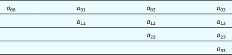
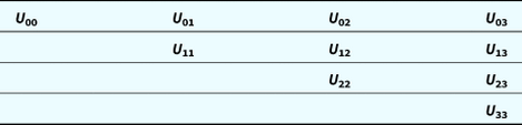
Points, lines, planes, and solids are respectiive 0D, 1D, 2D, and 3D geometric elements that will serve as the building blocks of shapes.They are situated in the 3D space, but less than 3D elements could be situated in less than 3D spaces as well. A line can be in the space, but also on an infinite plane or an infinite line. At the minimum, a point can be situated on a point, which is a 0D space. In general, a geometric element is characterized by its dimensionality and the dimensionality of the space it is defined in. Typically, a geometric element of dimension i defined in the space of dimension j ≥ i is denoted by aij with all the combinations shown in Table 1.
Geometric elements a ij of dimension i defined in the space of dimension j (j ≥ i) enumerated

It is clear from the table that the minimum space (in terms of its dimensionality) in which a single geometric element can be defined is of the same dimension as the geometric element itself. Elements defined in their minimum spaces are diagonal geometric elements as they appear on the diagonal of the table. The minimum space for a set of geometric elements could be as small as the minimum space of one of the elements and as big as the 3D space. For example, the minimum space for two collinear lines is 1D, for two parallel or two intersecting lines is 2D, while for two skew lines is 3D. If the minimum space of a nonempty set of geometric elements is the same as the minimum space of one of its elements, then it is a diagonal set and the space is a diagonal space. It is easy to see that in such a set all elements have the same minimum space. For example, the set of all solids is diagonal, but so is a set of collinear lines.
Boundaries of geometric elements
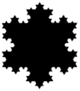
Boundaries outline geometric elements. Each geometric element is delineated by a finite collection of geometric elements one dimension smaller than itself. Two endpoints delineate a line, a polygon delineates a plane, and a closed polyhedral surface delineates a solid. Points do not have boundaries and lines have two-point boundaries. Given that each geometric element of dimension greater than 0 has infinitely many geometric elements embedded in it, the boundary of a geometric element of dimension greater than 1 can be described by an infinite set of geometric elements. However, the fact that there are also finite descriptions qualifies it as a boundary. There are figures with finite areas and infinite boundaries, that is, boundaries that cannot be described by finite sets. For example, the Koch snowflake in Figure 1 is a finite area planar figure which may have a fractal boundary with an infinite number of lines.
Koch snowflake: a finite area planar figure which may have an infinite fractal boundary.

Calculating with geometric elements
Geometric elements could be related in many ways. One could be embedded in or be coincident with another element or the two could overlap or touch. There are numerous other relations but these four play important roles when calculating with geometric elements. The most important relation is embedding. Intuitively, given two lines, the first line is embedded in the second one, if the result of drawing one on top of the other is the second line. The first line appears to be a part of the second one. The embedding relation is a partial order ≤ on a set of geometric elements of the same kind – that is, the elements of the same dimension defined in the same space. Note that this implies that only lines could be parts of lines, planes parts of planes, and solids parts of solids. A point can be coincident with a line but not its part. However, for a ≤ b to hold, where a and b are geometric elements, being of the same kind is not enough. There is another necessary – but not sufficient – condition: set {a, b} must be diagonal.
For points, partial order is identity. A point is a part of another point if the two are identical. That is if a ≤ b, then b ≤ a and a = b, where a and b are points. Note that for points, all diagonal sets are singletons.
Armed with partial order we may proceed to define Boolean operations: product, sum, difference, and symmetric difference – for geometric elements of the same kind belonging to the same diagonal set.
For points defined on a point (0D space), sum and product are always defined and equal to the only point, which is both the smallest and the greatest element. In contrast, difference and symmetric difference are never defined. Points defined in 1D, 2D, and 3D spaces have sum and product only if the points that are arguments are identical. In contrast, difference is only defined if the arguments are different points, while symmetric difference is never defined. Geometric elements of higher dimension have more elaborate behavior in calculations. Operations for lines planes and solids are defined below.
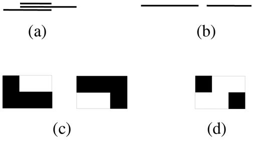
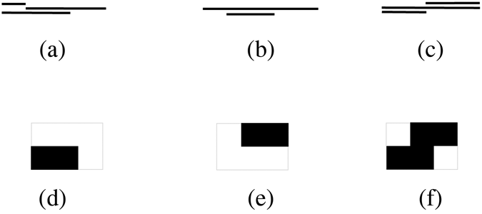
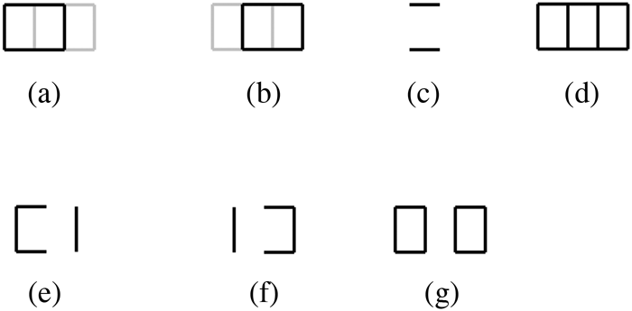
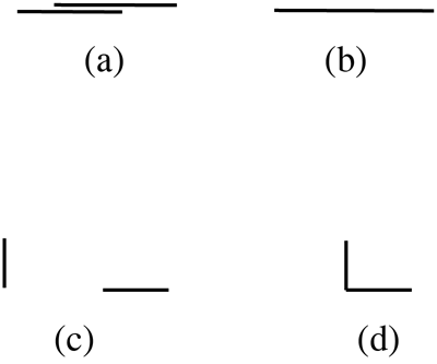
Product: a⋅b = c exists if c is the greatest common part of a and b. That is c ≤ a and c ≤ b so that set {a, b, c} is diagonal. Given the lines in Figure 2a, the top one is the product of the middle and the bottom line. Two lines in (b) belong to a diagonal set but do not have the product as there is no line that is part of both. It is clear from the definition and examples that for a⋅b to be defined a and b must have common parts – that is, overlap – however, this is not sufficient for planes and solids. For example, two overlapping L-s (c) do not have a product. The greatest common part is missing, as we end up with two incomparable elements (d).
Product: the top line is the product of the other two (a); there is no product of the two lines (b); there is no product of the two overlapping L-s (c) as there is no smallest common part (d).

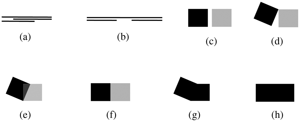
Sum: a + b = c if c is the smallest geometric element with both a and b as parts (1), and there is no part of c that does not share parts with a or b (2). If sum exists, then a ≤ c and b ≤ c so that set {a, b, c} is diagonal. Given lines in Figure 3a, the top one is the sum of the middle and the bottom line. In contrast, with lines (b) the top one is the smallest line with the bottom two as parts, but it is not their sum. It satisfies condition (1), however, the gap between the bottom lines can accommodate infinitely many lines that violate condition (2). Both conditions (1) and (2) are required only for lines. For planes and solids, condition (1) is sufficient. For example, neither planes (c) nor planes (d) satisfy (1) and cannot be summed. In contrast, planes (e) and planes (f) do satisfy (1) so that (g) and (h) are their respective sums. The sums exist because planes overlap in the first case and touch in the second.
Sum: top line is the sum of the other two (a); top line is not the sum of the other two (b); pairs of planes (c) and (d) do not have sums; pairs of planes (e) and (f) and their respective sums (g) and (h).

The touch relation could now be defined: geometric elements touch if their sum exists, but their product does not.Footnote 4
Difference: a – b = c exists if c is the greatest part of a that does not share parts with b. Given lines in Figure 4a, the top line is the result of subtracting the middle line from the bottom one. The same result we get if the middle line is subtracted from the top one and we get the middle line if the two arguments swap their places. That is, a – b = a and b – a = b if the two do not have common parts. There is no difference defined for lines (b) as we end up with two or no geometric elements depending on the order of arguments. There is another, somewhat unintuitive, requirement stemming from the Boolean nature of the operations. As there is no greatest or smallest geometric element, difference is defined using relative complements. It is the unique complement of b relative to the interval [b, a + b]. Thus, the difference could only be defined if a + b is defined. This is stricter than the usual diagonal set requirement.
The top line (a) is the result of subtracting the middle line from the bottom, or if the middle line is subtracted from the top one, and the middle line is the result of arguments swapping their places; there is no difference or symmetric difference for two the lines (b); each of the three lines (c) is the symmetric difference of the other two; the two overlapping L-s in Figure 2c yield two possible differences (d) and (e) and the symmetric difference (f).

Symmetric Difference: a ⊕ b = c exists if c is the greatest geometric element with each of its parts being either part of a or b, but not of both. For example, each of the three lines in Figure 4c is the symmetric difference of the other two. In contrast, lines (b) do not have the symmetric difference as two different lines satisfy the definition. Like the other operations, the symmetric difference is only defined for diagonal sets of arguments.
Although the operations above are Boolean in nature, some of the standard Boolean identities do not hold. For example, the definition of difference as the unique complement of a⋅b relative to the interval [a⋅b, a], which is equivalent to the one given before, does not hold if a⋅b is not defined although the difference may be defined. Similarly, if a – b exists, then a – b = a – (a⋅b) should hold. For example, the two overlapping L-s in Figure 2c yield two possible differences, as shown in Figure 4d,e. However, the identity does not hold for either of the differences because the product of the L-s is not defined. Likewise, the symmetric difference of the two L-s is (f), which is the following standard identity a ⊕ b = (a – b) + (b – a). However, another standard identity a ⊕ b = (a + b) − (a⋅b) does not hold for the lack of product.
Note that the geometric elements that are results of the operations above have finite boundaries because the elements that are the arguments of the operations have finite boundaries.
Set Iij of all geometric elements of dimension i defined in the space of dimension j together with operations ⋅, +, −, and ⊕ forms partial algebra Iij – which is partial because Iij is not closed under the operations.
Shapes
In the previous section, we were dealing with single geometric elements which are building blocks of shapes. Intuitively, shapes are collections of such elements like the collection of lines that makes a rectangle. Nevertheless, shapes will be defined here without relying on these intuitions. Rather, the formal conditions under which partial algebras of geometric elements evolve into algebras of shapes will guide the definition.
Defining shapes
Calculations with geometric elements are purely spatial: one starts with two geometric elements and transforms them into one usually different than both – but occasionally equal to one of them. Such a transformation depends on a spatial relation between geometric elements and may not always be possible. In contrast, nonspatial or symbolic calculations are always possible as they typically involve just repacking geometric elements while leaving them intact. One may take two elements from two packages and place them into one: {a} ∪ {b} = {a, b}; or may take some elements out of a package and not worry if the package ends up empty: {a, b}\{a, b} = {} = Ø. The packages are more important than the elements they contain so the latter are as good as symbols. In order for calculations with geometric elements to always be defined, Iij should be extended to include nonspatial (set) operations. Consequently, geometric elements are replaced with sets of geometric elements of the same kind, or shapes. Shapes are combinations of the spatial and nonspatial. The spatial is what matters the most while the nonspatial is there for closure, that is, to be able to calculate and always get the result.
For example, one cannot make a line out of the two lines in Figure 2b so the sum from I 11 fails. However, if each line is seen as a one-line shape, then the set union produces a two-line shape and we have the sum. Similarly, if the top line in Figure 4b is subtracted from the bottom one, no geometric element is left, and the difference fails. Not so if the two lines are shapes. The difference produces a shape with no geometric elements, just an empty set.
Geometric elements forming a shape must, be of the same kind, and occupy a finite chunk of space. Because there are infinitely many geometric elements embedded in a single geometric element – if its dimension is greater than 0 – different sets, including infinite ones, of geometric elements may represent the same shape. An infinite set may represent a shape if there is at least one finite set representing the same shape. The following proposition establishes bounds for such sets.
Proposition 1: Let a and A be sets of geometric elements defined in Iij and confined to a finite chunk of space. Let a be finite with sums being defined only for pairs of identical elements (i) and let A be the set of all elements that are parts of elements of a, or A = {x ≤ y | y ∈ a} (ii). The following holds:
(1) a is the set of maximal geometric elements of A,
(2) a represents a shape, and
(3) A is the set of all geometric elements embedded in the shape represented by a.
Proof: From (i), a is a set of maximal elements, and from (ii), a ⊆ A so that these are also maximal elements of A, which proves (1). a must have a finite boundary to be a shape. Because a is finite and so are the representations of boundaries of elements of a, the union of these representations is finite and is a representation of the boundary of a, which proves (2). Assume (3) does not hold so that there is a geometric element z embedded in the shape represented by a such that z ∉ A. Thus, z must be a sum of parts of different elements of a. From (i), no such sum exists so that (3) holds.
Sets a and A are, in terms of their cardinalities, respective minimal and maximal sets representing the same shape. The former one is the ideal shape representation because it is unique and compact which leads to the following three equivalent definitions of shape.
A shape occupies a finite chunk of space and is:
(1) A finite set of geometric elements defined in Iij such that only pairs of identical elements have sums.
(2) A finite set of maximal geometric elements defined in Iij.
(3) A finite subalgebra of Iij with sums and products defined only for identical elements.
Note that subset X of partial algebra Iij is its subalgebra if every sum (product) of elements of X which is defined is also an element of X.
Any finite set of geometric elements from Iij, occupying a finite chunk of space, may be represented as a shape.
Proposition 2: Let C be such a set and let cl +(C) be its closure under sum, where cl + is a closure operator on the set of subsets of C,℘(C). Set a of maximal elements of cl +(C) is a shape represented by C.
Proof: Because C is finite cl +(C) is finite and there are elements e∈cl +(C) such that for every c∈cl +(C) e + c = e or is not defined. The set of all elements like e is a and because they are maximal with respect to one another a is a shape. Each element of C is either part of or equal to an element of a because a is the set of maximal elements of cl +(C) so that a is the shape represented by C.
The proposition holds for infinite C provided that a exists and is finite and that for every x∈C there is y ∈ a such that x ≤ y. A good example of such a set is A from proposition 1.
Calculating with shapes
Calculations with shapes are combinations of spatial calculations, which alter geometric elements, and nonspatial ones, which just group them. Unlike spatial calculations with geometric elements, which may not always be defined, calculations with shapes always result in shapes.
As with geometric elements operations for shapes are Boolean and depend on the partial order among shapes. The latter is defined as follows.
The Subshape (or a part) a of shape b, or a ≤ b, is a shape where for every x ∈ a there is y ∈ b such that x ≤ y.
The smallest shape is an empty shape which is an empty set of geometric elements denoted by 0. An empty shape is a part of every shape. Note that there are different empty shapes as these are empty sets of elements from different Iij partial algebras.
The subshape relation is pivotal in defining operations on shapes, but for calculating with them we also rely on operations for geometric elements.
It is important to note that the operations below are defined for shapes occupying the same finite chunk of space. For example, two shapes that are an infinite distance apart cannot be summed. It could be argued that this requirement is unnecessary as “infinite distance” is nowhere to be found in nature, however, some of our representational tools do allow for it. Such an example is provided on page 6 (right column).
Sum: a + b is the smallest shape which has both a and b as parts.
Proposition 3: The sum of shapes a and b is the set of maximal elements of cl+(a ∪ b).
Proof: Per Proposition 2, set x of maximal elements of cl+(a∪b) is the shape represented by a∪b. Every element of x is either the sum of elements of both a and b, or is equal to an element of a or b. Thus, x is the smallest shape that includes both a and b as parts or x = a + b.
The sum could be calculated recursively via the following procedure, which uses the sum from Iij.
Procedure 1:
-
Initial values: A0 = a, B0 = b, i = 1, 2,…card(b)Footnote 5
-
Recursive step: Bi = Bi− 1 \ {b}, where b ∈ Bi− 1,
-
C = {x if x + b is not defined | x ∈ Ai− 1},
-
D = {x + b | x ∈ Ai− 1 \ C},
-
c = Σ (D ∪ {b}),
-
Ai = C ∪ {c}
-
-
Result: a + b = Acard (b)
For i = 1, we remove element b from b (line 1 of the recursive step) and partition a into set C of elements which do not sum with b and a set of ones that do (Ai− 1\C), which are then summed with b to get D (lines 2 and 3). D is augmented with b – just in case Ai− 1\C was empty – and summed to create geometric element c. All elements of D include b as a part so that their sum is defined. Element c is included in set C of elements which do not sum with b to create Ai. The process is continued until all the elements of b are exhausted (Bcard (b) = Ø). Note that each Ai is a shape – a set of maximal elements – and so is the result Acard (b). The set Uij of i-dimensional shapes defined in the j-dimensional space closed under + and ⋅ is a relatively complemented distributive lattice ordered by the subshape relation. It features an empty shape as the smallest element while lacking the greatest one. Being distributive makes its relative complements unique, enabling the definition of the difference operation.
Difference: a – b is the relative complement of b with respect to interval [0, a + b], or dually the relative complement of a⋅b with respect to interval [0, a]. It is the greatest shape made only of parts of a which have no parts that are parts of b.
Difference could be calculated recursively via the following procedure that utilizes the difference of Iij.
Procedure 2:
-
Initial values: A0 = a, B0 = b, i = 1, 2,…card(b)
-
Recursive step: Bi = Bi− 1 \ {b}, where b ∈ Bi− 1,
-
C = {x if x – b is not defined | x ∈ Ai− 1},
-
D = {x – b | x ∈ Ai− 1 \ C},
-
Ai = C ∪ D
-
-
Result: a – b = Acard (b)
Product: a⋅b is the greatest shape embedded in both a and b. To calculate it, we rely on the difference for shapes which is related to the product via a⋅b = a – (a – b).
Symmetric Difference: a ⊕ b is the greatest shape having only parts of a that have no parts that are parts of b and parts of b that have no parts that are parts of a. To calculate it, one may use – and + with formula a ⊕ b = (a – b) + (b – a) or equivalently by using –, +, and ⋅ with a ⊕ b = (a + b) – (a⋅b).
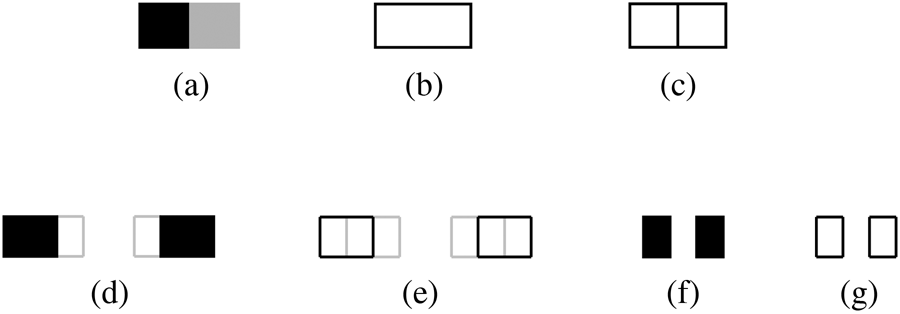
For example, the two shapes in Figure 5a have product (b), sum (c), difference (d), another difference (e), and symmetric difference (f).
Shape operations: two shapes (a) and (b) have the product (c), sum (d), difference (e), another difference (f), and symmetric difference (g).

Boundaries of shapes
We established earlier that the boundary of a geometric element may be represented by a finite set of geometric elements one dimension lower than the original element. However, proposition 2 allows for a more precise characterization of the boundary.
Boundaries of geometric elements are shapes one dimension lower than the elements because the boundary of an i-dimensional geometric element can be represented by a finite set of (i−1)-dimensional geometric elements it can, according to proposition 2, be represented as a shape.
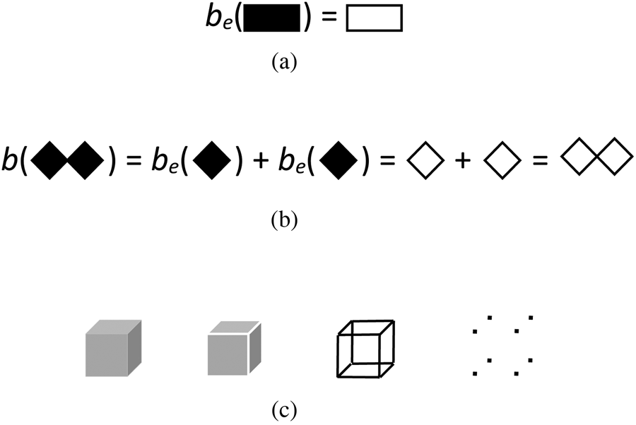
This allows for a unique and compact representation of boundaries and introduction of boundary operator be: Iij → Ui− 1j, where Ui− 1j is the set of (i − 1)-dimensional shapes defined in the j-dimensional space. The boundary operator takes a geometric element from Iij to its boundary which is a shape in Ui− 1j, or y = be(x), x ∈ Iij, y ∈ Ui− 1j. For example, the identity in Figure 6a shows operator be turning a quadrilateral planar geometric element into a set of four maximal lines or a linear shape which is a boundary of the planar element. Because shapes are sets of maximal geometric elements, boundaries are sums of the boundaries of the elements. Consequently, the boundary operator for shapes b: Uij → Ui− 1j is defined as b(a) = Σx ∈a be(x) where b(a) ∈ Ui− 1j, a ∈ Uij and x ∈ Iij. Identity (b) shows how this works for a planar shape having two maximal geometric elements.
Boundary operators: identity (a) shows operator be turning a quadrilateral planar geometric element into a linear shape which is its boundary; identity (b) shows operator b turning a two-element shape into its linear boundary by summing the boundaries of the elements; sequence (c) of shapes a cube and boundaries obtained by recursive applications of operator b.

Boundaries of shapes are shapes one dimension lower than the original shapes. They are sums of the boundaries of maximal elements representing shapes.
For example, the sequence of shapes in Figure 6c has a 3D solid cube, its boundary which is a 2D shape consisting of 6 planar squares, with a 1D boundary consisting of 12 lines, and its boundary a 0D shape having 8 points, respectively. It is a chain of boundaries of a 3D shape starting with the first-order 2D boundary (or simply the boundary), followed by the second-order 1D boundary, which is the boundary of the first-order boundary, and ending with the third-order 0D boundary, which is the boundary of the second-order boundary. More formally:
m-order boundary of shape a ∈ Uij is shape bm(a) ∈ Ui−mj, m ∈ {0, 1, … i} is defined recursively by b 0(a) = a, bn +1(a) = b(bn(a)).
There is a trivial, but nicely sounding proposition stemming from this definition.
Proposition 4: All shapes are m-order boundaries of shapes.
Calculations with shapes do not mirror calculations with their boundaries as the two are not isomorphic. For example, for the two singleton shapes in Figure 7a, the boundary of their sum (b) is different than the sum of their boundaries (c). The only exception is the operation of symmetric difference when applied to shapes sharing the same diagonal space.
Calculations with shapes and boundaries: two shapes (a), the boundary of their sum (b), and the sum of their boundaries (c); shapes (d) with their boundaries (e) have symmetric difference (f) with boundary (g).

Proposition 5: The boundary of the symmetric difference of two diagonal shapes sharing the same diagonal space is the symmetric difference of their boundaries, or b(a ⊕ b) = b(a) ⊕ b(b) where a, b ∈ Uii (Earl, Reference Earl1997; Krishnamurti and Stouffs, Reference Krishnamurti and Stouffs2004).
Proof: Possible spatial relations between a and b determine how parts of their boundaries are affected by a ⊕ b. A part of the original boundary should be removed if there is either a shape or an empty shape on both of its sides (i) and it should be preserved otherwise (ii). If b(a) ⋅ b(b) = 0 and either a ⋅ b = 0 or b < a or a < b, then a ⊕ b is a + b or a – b or b – a, respectively. In all three cases, boundaries of a and b satisfy (ii) and should be preserved which b(a) ⊕ b(b) = b(a) + b(b) does so that b(a ⊕ b) = b(a) ⊕ b(b) (iii) holds. If b(a) ⋅ b(b) ≠ 0 and either a ⋅ b = 0 or b < a or a < b, then a ⊕ b is a + b or a – b or b – a, respectively. In all three cases, b(a) ⋅ b(b) satisfies (i) and should be removed which b(a) ⊕ b(b) = [b(a) + b(b)] – [b(a) ⋅ b(b)] does so (iii) holds. If a ⋅ b ≠ 0 and b(a) ⋅ b(b) = 0, then a ⊕ b removes a ⋅ b so that b(a ⋅ b) satisfies (ii) and should be preserved. The remaining parts of boundaries b(a) – b(a ⋅ b) and b(b) – b(a ⋅ b) also satisfy (ii) so that both b(a) and b(b) should be preserved which b(a) ⊕ b(b) = b(a) + b(b) and again (iii) holds. This exhausts all the possible spatial relations between a and b and completes the proof.
For example, shapes in Figure 7d with their respective boundaries (e) have symmetric difference (f) with boundary (g). The latter is also the symmetric difference of boundaries of the original shapes. Restriction to diagonal shapes is necessary to avoid situations where the products of boundaries are parts of new boundaries like, for example, the surface of cube Figure 6c with the boundary made of lines that are products of boundaries of the adjacent faces. Because products are never parts of symmetric differences proposition 5 does not hold.
Proposition 5 can be generalized to include different order boundaries.
Proposition 6: The m-order-boundary of symmetric difference of two diagonal shapes sharing the same diagonal space is the symmetric difference of their m-order boundaries, or bm(a ⊕ b) = bm(a) ⊕ bm(b), where a, b ∈ Uii, and m ∈ {0, 1, … i} (see page 9 (left column) of the proof).
The corollary below extends proposition 6 to nondiagonal shapes of a certain kind.
Corollary: Let shapes a, b ∈ Uij be m-order boundaries of diagonal shapes from Ujj, where 1 ≤ i < j and m = j – i, then b(a ⊕ b) = b(a) ⊕ b(b) holds.
Proof: Let a = bm(a′) and b = bm(b′) so that a ⊕ b = bm(a′) ⊕ bm(b′) = bm(a′⊕ b′) in accordance with proposition 6. Now, b(a ⊕ b) = b(bm(a′⊕ b′)) = bm + 1(a′⊕ b′) = bm +1(a′) ⊕ bm +1(b′) =b(b m(a′)) ⊕ b(b m(b′)) = b(a) ⊕ b(b) in accordance with proposition 6 and the definition of m-order boundaries.
Propositions and the corollary above are global in nature as they consider shapes of certain kinds without considering their spatial relations. Sharper results could be achieved by considering some local properties. For example, the corollary of proposition 6 is sharpened by the proposition below (which is given without the proof).
Proposition 7: Let the product of shapes a, b ∈ Uij be the m-order-boundary of a diagonal shape from Ujj, where 1 ≤ i < j and m = j – i, then b(a ⊕ b) = b(a) ⊕ b(b) holds.
Algebras of shapes
Algebras of shapes (Stiny, Reference Stiny1991, Reference Stiny1992) provide the framework for calculations with shapes. They are formalizing the design practice by modeling what designers do when they design. The process of drawing, outlining, or erasing shapes is handled well with the Boolean operations above. Designers also move, scale, and otherwise transform shapes in order to achieve different spatial relations. This cannot be modeled with Boolean operations. For that Uij must be closed under similarity transformations. The latter form an algebra of their own: a group. An algebra for shapes must include both a Boolean lattice and a group.
Two-sorted algebras of shapes
An algebra of shapes should have a Boolean part to handle the structures of shapes and a group part to deal with their symmetries (Krstic, Reference Krstic1999, Reference Krstic and Gero2014).
The Boolean part has set Uij of shapes, occupying a finite chunk of space, which together with Boolean operations forms a relatively complemented distributive lattice with the least element, but without the greatest one. Such a structure is due to its Boolean properties also known as Generalized Boolean Algebra (Birkhoff, Reference Birkhoff1993).
The group part has set Tij of similarity transformations that can act on i-dimensional shapes defined in a j-dimensional space. Set Tij is closed under group operations of composition °, inverse −1, and identity ι, to form group Tij. This structure allows for calculating with transformations. For example, simple transformations could be combined to create more complex ones, or an inverse of a transformation could be created to undo an erroneous move.
Boolean and group parts are connected via the operation of group action (): Tij × Uij → Uij where shape a is acted upon by transformation t to produce the transformed shape t(a).
Note that Tij need not be the similarity group of transformations. It could be any group that can act on shapes like the rigid body, Euclidean, affine, or some subgroups of these, or even some unusual ones as a group with shapes as elements (Krstic, Reference Krstic1999).
Boolean and group parts are combined in a two-sorted algebra Uij with carrier {Uij, Tij} having elements of two different sorts – shapes and transformations – and signature {⋅, +, c, ⊕, °, −1, ι, ()} with Boolean and group operations as well as the group action. Algebras Uij are enumerated and sorted in Table 2 based on the dimensionality of geometric elements making their shapes (i) and the dimensionality of the space the latter are defined in (j). The table resembles Table 1 of geometric elements. For example, algebras with shapes defined in the minimum space of their geometric elements appear on the diagonal of the table, the same way the elements appeared in the previous table. The geometric elements were diagonal, and the algebras are diagonal operating on diagonal shapes in diagonal spaces.
Algebras Uij enumerated and sorted based on the dimensionality of geometric elements making their shapes (i) and the dimensionality of the space the latter are defined in (j)

As mentioned earlier, a shape has to be confined to a finite chunk of space and the same requirement holds for set Uij of shapes. Although infinite distances are common in mathematics, they do not appear in nature so that these constraints seem unnecessary. However, there are some methods of 3D object representation that include infinite distances.
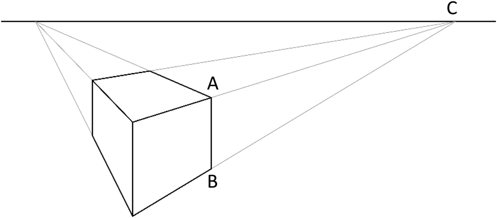
For example, the drawing in Figure 8 includes lines in the plane which should belong to a U 12 algebra so that triangle ΔABC is a shape – an element of U 12. There are also (labeled) points A, B, and C which are shapes in a U 02 algebra and so is their sum. In contrast, the drawing can be seen as a perspective representation of a cube. As such it belongs to a U 12 algebra which is now closed under projective transformations in place of the similarity ones. Triangle ΔABC is not a shape in this new algebra. Its sides AC and BC are infinite in length because point C is a vanishing point at infinity for a pencil of parallel lines. Points A, B, and C are now shapes in a U 02 algebra closed under projective transformations. However, their sum is not a shape because it has three points as maximal elements where one is infinitely distanced from the other two. So, it seems that the finite chunk containment requirement should stay after all.
Perspective drawing of a cube.

Combining algebras of shapes
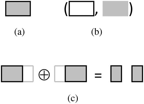
Shapes in practice often come as compound, having geometric elements of different kinds like the shape in Figure 9a, which has four lines and a planar segment. The lines belong to U 12 while the planar segment belongs to U 22 so that the shape must belong to a combination of the two algebras. A standard algebraic combination is the direct product of component algebras which have the same signatures. Direct product U 12 × U 22 of U 12 and U 22 is a two-sorted algebra of compound shapes with carrier {U 12 × U 22, T 12 × T 22}, which is the Cartesian product of the component carriers and operations defined componentwise. Shape (a) is represented by the ordered pair (b) where the first element is in U 12 and the second in U 22. The componentwise symmetric difference of two compound shapes (a, u), (b, v) ∈ U 12 × U 22 is (a, u) ⊕ (b, v) = (a ⊕ b, u ⊕ v) with an example of such calculations depicted in Figure 9c.
Compound shapes: shape (a) with linear rectangle and a planar segment represented by ordered pair (b) with first element belonging to U 12 and to U 22.

Likewise, the action of compound transformation (t 1, t 2) ∈ T 12 × T 22 on compound shape (a, b) ∈ U 12 × U 22 is (t 1, t 2)((a, b)) = (t 1(a), t 2(b)) ∈ U 12 × U 22.
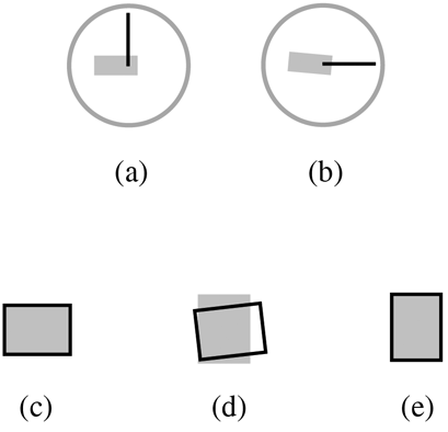
For example, the clockface in Figure 10a showing 9:00 is defined in U 12 × U 22. It shows 9:15 (b) after the action of transformation (rot(−90°), rot(−90/12 = −7.5°)) ∈ T 12 × T 22, where rot(x) is the rotation of x degrees around the origin.
Compound algebras: clockface (a) defined in U 12 × U 22 is showing 9:00; it shows 9:15 (b) when transformed by (rot(−90°), rot(−7.5°)) ∈ T 12 × T 22; shape (c) rotated in a direct product algebra (d) and in a sum of algebras (e).

Another combination of algebras is their sum. Unlike direct product, which is in the domain of universal algebra, sum is particular to algebras of shapes (Krstic, Reference Krstic1999, Reference Krstic and Gero2014). It is based on a subdirect product, that is, a subalgebra of a direct product that enumerates all elements of the component algebras, but not all of their combinations. The sum of two shape algebras is a subdirect product that enumerates all shapes of the component algebras as well as all their combinations but allows only combinations of equal transformations. Sum does not restrict the Boolean part but requires for all components of compound shapes to be transformed in the same way. This preserves the integrity of compound shapes in calculations. For example, the compound shape in Figure 10c could be rotated in the direct product algebra so that its boundary is off (d) however, this cannot happen with the sum of algebras where both the shape and its boundary are rotated in the same way (e).
Decomposing algebras of shapes
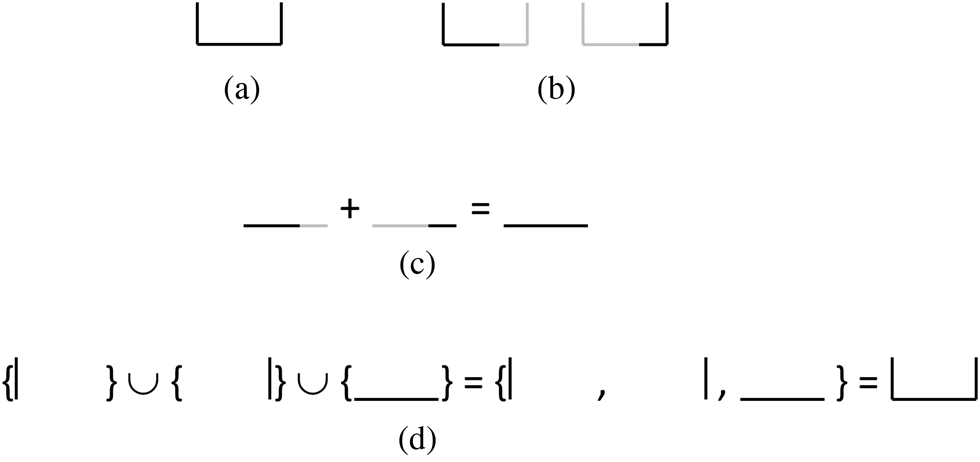
As previously shown, occupying the same diagonal space is the necessary condition for two geometric elements to be able to spatially interact. However, they must overlap or at least touch for their interaction to result in new geometric elements. All shapes in a diagonal algebra share the same diagonal space as, for example, the two lines in Figure 11a, which are singleton shapes from U 11. The sum of the lines is a spatial calculation as it results in a longer line (b). In contrast, two singleton shapes (c) defined in U 12 have sum (d) which is their set union. This is a nonspatial calculation with no new geometric elements produced. Calculations are usually combinations of the spatial and nonspatial ones. For example, the shape in Figure 12a, defined in U 12, is the sum of shapes (b). This calculation has a spatial part (c) and a nonspatial one (d). Note that + from U 12 acts as sum from U 11 in the spatial part of the calculation and as set union in the nonspatial part. This means that instead of calculating with shapes in U 12 we may calculate with their parts in diagonal algebras U 11 and take the union of the results of these calculations. To take this further, we need to utilize special types of shape decompositions.
Two lines (a) defined in U 11 and their sum (b); two lines (c) defined in U 12 and their sum (d).

Spatial and nonspatial: shape (a) is the sum of shapes (b); this calculation has a spatial part (c) and a nonspatial one (d).

Natural and diagonal decompositions of shapes
A shape could be decomposed into shapes that are its parts. Given shape a, set A of its parts is a decomposition of a if it is finite and sums up to a, or ΣA = a. Set A is a discrete decomposition of a if for each x, y ∈ A and x ≠ y, x⋅y = 0. There is a unique discrete decomposition of each shape that stems from the shape definition.
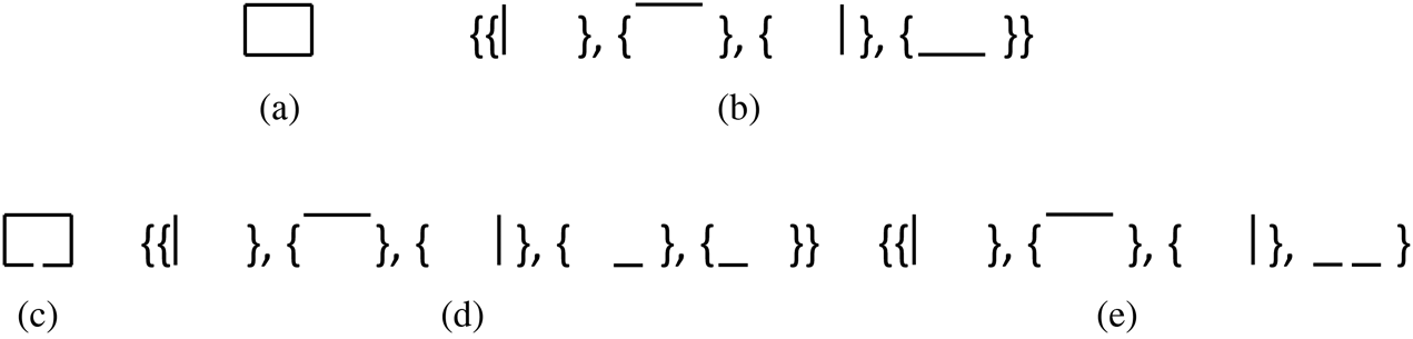
The natural decomposition of shape a ∈ Uij is set na with elements that are singleton shapes of maximal geometric elements which define a, or na = {{x}| x ∈ a}. For example, the shape in Figure 13a has natural decomposition (b). Each shape has its unique natural decomposition. Because shapes which are elements of the decomposition are incomparable, their sum and union are equal, or Σna = ∪na = a.
Natural and diagonal decompositions: shape (a) and its natural decomposition (b); shape (c) and its natural (d) and diagonal (e) decompositions.

Each element of a natural decomposition is singleton shape, so its minimum space is a diagonal one. Two shapes belonging to the same algebra may have natural decompositions such that an element of one decomposition shares diagonal space with an element belonging to a different one. There could be several such pairs of elements. If the two shapes are arguments of some calculation, then calculations with elements sharing the same diagonal space could take place in the related diagonal algebra. This opens interesting possibilities, however, not without a problem. There is no guarantee for two elements of the same natural decomposition to be in different diagonal spaces. Fortunately, there is another discrete decomposition related to the natural one, which overcomes this problem.
The diagonal decomposition of a shape is a discrete decomposition in which each element is a diagonal shape and no two elements share the same diagonal space. The decomposition in Figure 13b is both natural and diagonal. In contrast, shape (c) has decompositions (d) and (e) as natural and diagonal, respectively.Footnote 6 Note that the last two shapes in the natural decomposition share the same diagonal space so they are replaced with their sum in the diagonal one. Going the other way, each nonsingleton shape of a diagonal decomposition should be replaced with its natural decomposition to get the natural decomposition of the original shape. Like natural decompositions diagonal ones are unique and also like natural decompositions they sum in a nonspatial way: Σda = ∪da = a. Let na and da be the respective natural and diagonal decompositions of shape a, then na ≤ da and card(da) ≤ card(na).Footnote 7
Now, we are in a position to break calculations with shapes into partial calculations carried on in diagonal algebras defined by the diagonal decompositions of the argument shapes. Let da and db be the respective diagonal decomposition of shapes a and b from Uij, and let shapes x ∈ da and y ∈ db share the same diagonal space. That is to say that set {x, y} is diagonal, or ordered pair (a, b) is diagonal, or shapes x and y are co-diagonal. Partial calculation x * y, where * stands for ⋅, +, −, or ⊕, could be carried on in Uij, but also in a diagonal algebra Uii defined in the space that x and y share. Different such pairs may exist and for each of them the above partial calculation is carried on in an appropriate diagonal algebra. The same could be extended to elements that could not be paired by simply pairing them with appropriate empty shapes. Finally, the union of the results of such partial calculations is equal to a * b. So instead of doing a calculation in Uij we did several simpler calculations in different Uii algebras.
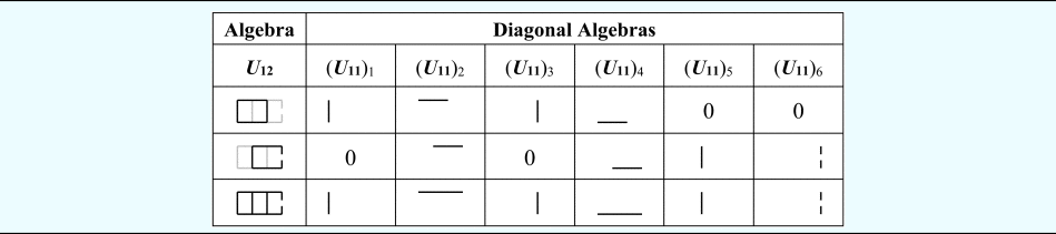
For example, the calculation in Figure 14 carried out in U 12 can also be done in six diagonal algebras U 11 by using diagonal decompositions of the argument shapes, as shown in Table 3.
Calculation carried out in U 12.

Example, of a calculation with shapes carried out in U 12 and also with diagonal decompositions of the argument shapes carried out in six diagonal algebras U 11

Shapes which are arguments of the calculation in U 12, as well as their diagonal decompositions spanning U 11 algebras, are shown in rows 3 and 4 of the table. Each diagonal decomposition spans four diagonal algebras and both decompositions span six algebras. The resulting shape of the calculation appears in the bottom row together with its decomposition which has nonzero elements in all six diagonal algebras. Calculations in (U 11)2 and (U 11)4, where decompositions of both argument shapes have nonzero elements, are spatial: they result in new shapes. The calculations in the rest of the algebras are nonspatial with the nonzero argument as the result. Note that the decomposition of the resulting shape is also diagonal.
Because diagonal decompositions are unique, we may introduce operator d: Uij → ℘(Uij) that takes a shape to its diagonal decomposition, or d(a) = da. The calculation above exposed an interesting property of diagonal decompositions, d(a + b) = d(a) + d(b), where + on the right side is carried out componentwise. This remains true for other Boolean operators (⋅, −, ⊕), which gives rise to an algebra of diagonal decompositions.
Algebras of diagonal decompositions of shapes
The uniqueness of diagonal decompositions – that is, their 1-1 relation to shapes – as well as the expressions like the one above render an algebra of diagonal decompositions isomorphic to an appropriate algebra of shapes. This is expressed by commutative diagram  ${\boldsymbol U}_{{{\boldsymbol ij}}\enspace} {}_{d}\!\! \mathbin{\lower.3ex\hbox{$\buildrel\textstyle\rightarrow\over {\smash{\leftarrow}\vphantom{_{\vbox to.5ex{\vss}}}}$}} \!\!{}^{_{\cup}} \ {{\boldsymbol X}_{{\boldsymbol ij}}}$, where Xij is an algebra of diagonal decompositions of shapes from Uij.
Table 3 may provide some guidance on how to do Boolean operations in Xij.
Let two shapes a and b defined in Uij be arguments of calculation a * b = c, where * stands for ⋅, +, −, or ⊕. To do the calculation with diagonal decompositions in place of shapes, we may use the following procedure.
Procedure 3:
1. Define diagonal decompositions of Uij implied by d(a) and d(b), that is, A = {Uii | x ∈ d(a), x ∈ Uii} and B = {Uii | x ∈ d(b), x ∈ Uii}.
2. Calculate sets of diagonal algebras which are in B but not in A or in A but not in B, that is,. A′ = B\A and B′ = A\B.
3. Augment decompositions d(a) and d(b) with empty shapes of algebras from sets A′ and B′, that is, d(a)′ = d(a) ∪ {0 ∈ Uii | Uii ∈ A′} and d(b)′ = d(b) ∪ {0 ∈ Uii | Uii ∈ B′} so that card(d(a)′) = card(d(b)′).
4. Calculate d(c)′ = {x * y | x ∈ d(a)′, y ∈ d(b)′, x, y ∈ Uii, Uii ∈ A ∪ B}.
5. Finally calculate d(c) = {x ∈ d(c)′ | x ≠ 0}.
Because a Uij algebra includes transformations, one would expect that a related algebra of diagonal decompositions includes them as well. However, it only handles the Boolean part while leaving the transformations to Uij. Diagonal decompositions and their algebras streamline spatial calculations with shapes by breaking them down into simpler calculations with parts of the shapes. The latter calculations are independent with respect to one another and could be done in parallel. The same approach may be used for checking the partial order among shapes by comparison of their parts done in parallel. A diagonal decomposition could easily be turned into the related natural decomposition – which is the standard maximal representation of a shape – and vice versa.
To showcase the utility of diagonal decompositions, we will use them to provide a rather elegant proof of proposition 6 – which has been left unproven on page 6 (left column).
Proof of Proposition 6: We will prove by induction on m validity of bm(a ⊕ b) = bm(a) ⊕ bm(b), where a, b ∈ Uii and m ∈ {0, 1, … i}. It trivially holds for m = 0 stating that a ⊕ b = a ⊕ b. Assuming that it holds for n, 1 ≤ n < m, we have to prove that it holds for n + 1. Because it holds for n, d(bn(a ⊕ b)) = d(bn(a)) ⊕ d(bn(b)) also holds. Now, let elements xa⊕b ∈ d(bn(a⊕b)), xa ∈ d(bn(a)), and xb ∈ d(bn(b)) of diagonal decompositions belong to the same diagonal algebra Ui −n i−n. Because these are diagonal shapes (*) b(xa⊕b) = b(xa) ⊕ b(xb) holds by proposition 5. Identities (*) hold for every diagonal algebra induced by the above diagonal decompositions. By summing all of these identities, we get (**) b(bn(a⊕b)) = b(bn(a)) ⊕ b(bn(b)) in accordance with the definition of shape boundaries. Identity (**) is bn +1(a ⊕ b) = bn +1(a) ⊕ bn +1(b) by the definition of m-order boundaries which completes the proof.
With the aid of diagonal decompositions, we were able to break the problem into smaller chunks for which proposition 5 holds and get the result by summing them back to shapes.
Direct sum representation of an algebra of shapes
In the calculations above – as specified by procedure 3, algebra Uij is de facto decomposed into a finite set of different diagonal algebras Uii each of which is tasked with a partial calculation. The union of the partial results is the final one. Each diagonal decomposition of a shape defined in algebra Uij induces the decomposition of Uij into a set of diagonal algebras Uii. The decomposition is relative to the shape as it is induced by the shape's diagonal decomposition which is unique. Thus, for each shape a ∈ Uij, there is the diagonal decomposition of Uij relative to a denoted by dij(a). However, many shapes could have the same diagonal decompositions of Uij. Let a, b, c ∈ Uij such that a and b are arguments and c is the result of a calculation carried out in Uij, then the decomposition relative to the calculation is dij(a) ∪ dij(b) while the decomposition related to the result of the calculation or dij(c) can be any subset of dij(a) ∪ dij(b) including the empty one.
For example, decompositions of algebra U 12 relative to shapes in the calculation in Figure 11f are {(U 11)1, (U 11)2, (U 11)3, (U 11)4} and {(U 11)2, (U 11)4, (U 11)5, (U 11)6} for arguments and {(U 11)1, (U 11)2, (U 11)3, (U 11)4, (U 11)5, (U 11)6} for the result – as shown in Table 3. The resulting decomposition is, in this case, the union of the argument ones, which is also the decomposition relative to the calculation itself.
Algebras of diagonal decompositions as they are defined so far are good enough for practical applications, however, to make them formally sound we need some more work.
For each calculation, Uij is decomposed into a finite set of Uii algebras which are considered components so that calculations are done componentwise. The pool of possible Uii algebras is infinite for all algebras with i < j. For diagonal algebras (i = j), it is a one-member family: the algebra itself. The pool of algebras is represented by the family (Uii)k ∈S, where S is an infinite indexing set.
For example, a U 12 algebra, with elements which are line segments in a plane has pool (U 11)k ∈S which is the set of diagonal algebras manipulating line segments on infinite lines coincident with that plane. Note that not all U 11 algebras are elements of (U 11)k ∈S but only those whose spaces are coincident with the space of U 12.
Diagonal algebra Uii is coincident with a Uij algebra if its space is coincident with that of Uij.
We can construct a direct product algebra from the diagonal algebras of (Uii)k ∈S:
 $$Q = \prod\nolimits_{{_k }_{{\in} S}} {{( {{\boldsymbol U}_{{\boldsymbol ii}}} ) }_k}.$$
Because S is an infinite set, Q is an infinite direct product with elements which are infinite tuples containing one element from each of the component diagonal algebras. Tuples with all but finitely many elements being 0 correspond to the diagonal decompositions of shapes. For example, the tuple corresponding to d(a), a ∈ Uij, will have shapes from d(a) at positions corresponding to diagonal algebras from dij(a) and empty shapes elsewhere. Such tuples form an infinite direct sum algebraFootnote 8 which is isomorphic to Uij.
Proposition 8: Every Uij algebra is isomorphic to the direct sum of diagonal algebras Uii which are coincident with Uij, or
 $${\boldsymbol U}_{{\boldsymbol ij}} = {\oplus} _{k\in S}( {{\boldsymbol U}_{{\boldsymbol ii}}} ) _k,$$
where the identity above holds up to isomorphism. Note that symbol ⊕ above denotes direct sum, however, it stands for symmetric difference everywhere else in the text.
The proposition above describes the diagonal decomposition of Uij which could also be seen as its direct sum representation. Note that infinite tuples are more elegant representations of shapes than diagonal decompositions. They both do the same job when calculating with shapes, however, the former do it in the standard componentwise way while the latter rely on a proprietary procedure (procedure 3). For i < j, we have an infinite direct sum, while for i = j, we have one component direct sum which is the original diagonal algebra with a twist: its elements are singletons containing shapes.
Like Uij the direct sum algebra is closed under similarity transformations. These involve spatial transformations carried out in diagonal algebras as well as (nonspatial) permutations of index set S.
Calculating with shapes and their boundaries
Proposition 5 opens the possibility for calculating with both shapes and their boundaries in parallel. This could be done in the framework of direct product algebra Uii × Ui −1i, however, some smaller algebras may provide a better fit. First, both shapes and their boundaries should be transformed in the same way so that (t, t) are the only ordered pairs of transformations allowed. Second, not all shapes from Ui −1i are boundaries of the shapes from Uii. A line in U 12 is not the boundary of any plane in U 22. Consequently, the set of boundaries of shapes from Uii is a proper subset of Ui −1i or b(Uii) ⊂ Ui −1i. According to proposition 5, set b(Uii) is closed under symmetric difference and could be elevated to an algebra Bi of boundaries of shapes from Uii. Now, a subdirect product UBi ⊂ Uii × Bi operating on compound shapes where shapes from Uii are matched with their boundaries from Bi, or UBi = {(x, b(x)) | x ∈ Uii, b(x) ∈ Bi}, i = 1, 2, or 3, provides an economical framework for parallel calculations with shapes and their boundaries. Calculations in UBi are carried out componentwise, or (a, b(a)) ⊕ (b, b(b)) = (a ⊕ b, b(a) ⊕ b(b)), where (a, b(a)), (b, b(b)) ∈ UBi. For example, the calculation in Figure 9c, when carried out in UB 2, accounts for both planar shapes and their linear boundaries. The new algebra is weaker than the standard algebras of shapes. It has only one operation – symmetric difference – and works with only one kind of shape – diagonal shapes. Symmetric difference is not that limited as it may act as the sum or as the difference depending on the context. For example, a ⊕ b = a + b if a⋅b = 0, a ⊕ b = a – b if a ≤ b, and a ⊕ b = b – a if b ≤ a. Calculations defining a shape grammar rule application depend on both sum and difference. Certain types of grammars like subtractive and collision-protecting ones provide the right context for symmetric difference to play both roles. Algebras UBi are therefore the right framework for such grammars to simultaneously generate shapes and their boundaries.
Boundary-paired diagonal decompositions and their algebras
So far, we have been following Krstic (Reference Krstic2001) in developing UBi algebras, but will now use devices developed in this paper to lift the restriction of UBi algebras to diagonal shapes.
First, the corollary of proposition 6 and proposition 7 allow for the immediate extension of proposition 5 to shapes which need not be diagonal, but either they or their products are m-order boundaries of diagonal shapes. Further extension – to (all) shapes – may be achieved via diagonal decompositions.
Unlike Bi set Bij ⊂ Ui −1j of boundaries of shapes from Uij cannot be elevated to an algebra. Instead, we approximate shapes from Uij with a special kind of diagonal decomposition.
The boundary-paired or b-paired diagonal decomposition of a shape is the diagonal decomposition in which every element is paired with its boundary. Because both the diagonal decomposition and boundary are unique for a shape so is its b-paired diagonal decomposition. Thus, we may introduce operator d′: Uij → ℘(Uij × Ui −1j) which takes a shape from Uij to its b-paired diagonal decomposition. Operator d′ is defined as d′(a) = {(x, b(x))| x∈d(a)}, a∈Uij. To go the other way, from b-paired diagonal decompositions to shapes and their boundaries, we make use of projection operators pru(d′(a)) = {x| (x, y)∈d′(a)} and prb(d′(a)) = {y| (x, y)∈d′(a)} so that a = ∪[pru(d′(a))] and b(a) = Σ[prb(d′(a))], where a∈Uij and b(a)∈Ui −1j. Like diagonal decompositions the b-paired ones form algebra UBij, however, this one has only one operation: symmetric difference ⊕. Like algebras for diagonal decompositions, UBij algebras handle only the Boolean part while leaving the transformations to Uij.
Proposition 9: Let d′(a) and d′(b) be b-paired diagonal decompositions of shapes a, b∈Uij. The following holds:
(1) Each element (x, b(x))∈d′(a) is an element of some UBi algebra.
(2) b-paired diagonal decompositions are closed under symmetric difference, or d′(a ⊕ b) = d′(a) ⊕ d′(b), and form algebra UBij.
Proof: If (x, b(x))∈d′(a), then x∈d(a) so that x∈Uii, for some Uii, therefore, (x, b(x))∈UBi, which proves (1). (2) follows from (1), the fact that d(a ⊕ b) = d(a) ⊕ d(b), and proposition 5, that is, b(a ⊕ b) = b(a) ⊕ b(b).
It follows from (1) that d′(a) implicitly defines a set A of UBi algebras to which its elements belong, or A = {UBi | x∈d′(a), x∈UBi}. Consequently, calculation d′(c) = d′(a) ⊕ d′(b) can be compartmentalized and carried on in parallel via a procedure not unlike the one for diagonal decompositions.
Procedure 4:
1. Define sets A and B of UBi algebras to which elements of d′(a) and d′(b) respectively belong, as well as their relative complements A′ = B\A and B′ = A\B.
2. Augment decompositions d′(a) and d′(b) with empty shapes of algebras from sets A′ and B′, that is, d′(a)′ = d′(a) ∪ {(0, 0)∈UBi | UBi∈A′} and d′(b)′ = d′(b) ∪ {(0, 0)∈UBi | UBi∈B′}.
3. Calculate d′(c)′ = {(x ⊕ u, y ⊕ v)|(x, y)∈ d′(a)′, (u, v)∈ d′(b)′, (x, y), (u, v)∈UBi, UBi∈A ∪ B}.
4. Finally, calculate d′(c) = {(x, y) ∈ d′(c)′ | x ≠ 0, y ≠ 0}.
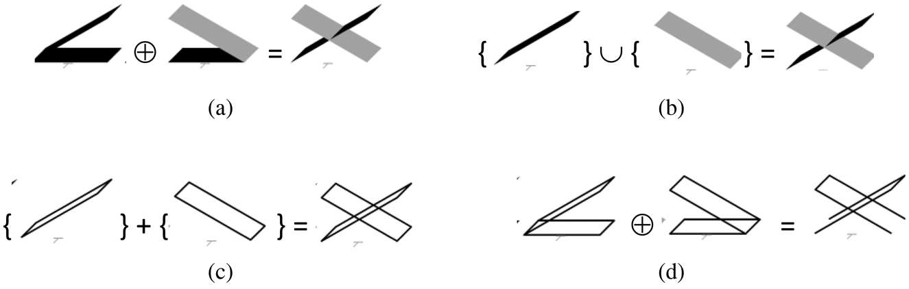
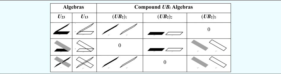
For example, Figure 15a depicts a calculation carried on in a U 23 algebra – where symmetric difference of a “smaller-than” and “greater-than” shape results in an “X” shape. Table 4 shows how the same calculation looks when done with b-paired diagonal decompositions in place of the shapes. Argument shapes, their boundaries, and their b-paired diagonal decompositions are in the third and fourth rows of the table while resulting shape, its boundary, and its b-paired diagonal decomposition occupy the fifth row.
Calculation in U 23 algebra (a); the resulting shape obtained from its decomposition by a nonspatial calculation (b) and its boundary by a spatial calculation (c); calculation carried out in U 13 yields an incomplete boundary (d).

Calculation in Figure 15a done with b-paired diagonal decompositions in place of the shapes. Argument shapes, their boundaries, and their b-paired diagonal decompositions are in the third and fourth rows of the table while resulting shape, its boundary, and its b-paired diagonal decomposition occupy the fifth row

The resulting “X” shape is obtained from its decomposition via nonspatial calculation (b). In contrast, spatial calculation (c) produces the boundary of “X”. Note that the original calculation (d) carried on in a U 13 algebra results in an incomplete boundary of “X”.
Generalization of UBi and UBij algebras
Based on proposition 6, we may extend b-paired diagonal decompositions to include m-order boundaries so that UBi and UBij algebras could manipulate multiple representations of shapes in parallel.
For example, the sequence of four shapes in Figure 6c may be seen as a solid cube represented by its faces, its edges, and its vertices. It could also be seen as a sequence of m-order boundaries b 0(a), b 1(a), b 2(a), b 3(a), where a is a solid cube belonging to a U 33 algebra. Let b be another shape, say another cube, from U 33, then in accordance with proposition 6 and definition of ⊕ the following holds:
-
bm(a + b) = bm(a) ⊕ bm(b), for a⋅b = 0,
-
bm(a – b) = bm(a) ⊕ bm(b), for b ≤ a,
-
bm(b – a) = bm(a) ⊕ bm(b), for a ≤ b,
-
bm(a ⊕ b) = bm(a) ⊕ bm(b), otherwise,
where m ∈ {0, 1, 2, 3}.Footnote 9 This means that we can meaningfully calculate with shapes while simultaneously accounting for their different representations. Algebras UBi and UBij could be extended to their respective generalized versions  ${\boldsymbol U}{\boldsymbol {B}^{\prime}}_{\boldsymbol i}$ and
 ${\boldsymbol U}{\boldsymbol {B}^{\prime}}_{{\boldsymbol ij}}$, to provide a framework for such calculations.
Elements of a  ${\boldsymbol U}{\boldsymbol {B}^{\prime}}_{\boldsymbol i}$ algebra are n-tuples (bk 1(a), bk 2(a), … bkn(a)) where k 1 = 0 < k 2 < ⋯ < kn ≤ i, and 1 ≤ n ≤ i + 1. The first element of the n-tuple is the shape itself (b0(a) = a) followed by an ordered – not necessarily complete – sequence of m-order boundaries. For example, the cube in Figure 6c may be represented by triplet (b 0(a), b 2(a), b 3(a)), that is, by itself, its edges and its vertices. Algebras
 ${\boldsymbol U}{\boldsymbol {B}^{\prime}}_{\boldsymbol i}$ are generalizations of both UBi and Uii algebras in the sense that for n = 2 and k 2 = 1,
 ${\boldsymbol U}{\boldsymbol {B}^{\prime}}_{\boldsymbol i}$ becomes UBi, and for n = 1, it becomes Uii. Calculations in
 ${\boldsymbol U}{\boldsymbol {B}^{\prime}}_{\boldsymbol i}$ are done componentwise as in UBi except that the number of components may be different.
Algebras UBij can be generalized in a straightforward fashion. Because their elements are b-paired decompositions with components belonging to different UBi algebras by replacing the latter with  ${\boldsymbol U}{\boldsymbol {B}^{\prime}}_{\boldsymbol i}$ algebras, we get
 ${\boldsymbol U}{\boldsymbol {B}^{\prime}}_{{\boldsymbol ij}}$ ones. Again, for n = 2 and k 2 = 1,
 ${\boldsymbol U}{\boldsymbol {B}^{\prime}}_{{\boldsymbol ij}}$ becomes UBij, and for n = 1, it becomes Uij.
Conclusion
Throughout the paper, we dealt with mathematics arising in the context of shape grammars theory. The latter started in the early 1970s with the introduction of shape grammars, as production systems capable of generating shapes, and evolved over the period of half a century into a formal design theory in which we analyze by seeing and calculate by drawing. We focused on algebras of shapes and particularly on their two-sorted version. In going from geometric elements and their partial algebras to shapes and their algebras, we followed Krstic (Reference Krstic1999) while introducing some improvements along the way like the two procedures for shape operations + and − based on partial operations for geometric elements.
We examined spatial and nonspatial calculations with shapes with an eye toward separating them. However, only geometric elements are combined in a purely spatial fashion. The closest the shapes get to this is when they belong to diagonal algebras. Diagonal decompositions are introduced to partition shapes so that each element of a decomposition belongs to a different diagonal algebra – implying a co-diagonal equivalence relation. This way all spatial calculations take place in diagonal algebras and may be done in parallel. The resulting diagonal decompositions are turned into shapes via simple nonspatial operations. Although this approach may be novel from the theoretical point of view the same notions have a long history. Forty years ago, Krishnamurti (Reference Krishnamurti1980) used the collinearity relation to partition linear shapes in the same way the diagonal decompositions do. He later extended it to shapes of higher dimension via the co-descriptor relation (Krishnamurti, Reference Krishnamurti1992). Stiny (Reference Stiny2006, pp. 202–204) got the same result with the coembeddedness equivalence relation and noted that such partitioning “is a nice way to store maximal elements in a computer”.
Boundaries of shapes were investigated and m-order boundaries introduced as consequences of recursive applications of the boundary operator. Proposition 5 is generalized to m-order boundaries and some other propositions related to standard boundaries stemmed from this generalization. Parallel computations with shapes and their boundaries are extended from diagonal shapes to (all) shapes. This required the introduction of b-paired diagonal decompositions of shapes as well as their algebras. Stiny (Reference Stiny2006, pp. 202–204) does similar calculations with shape boundaries by breaking shapes into parts for which proposition 5 holds.
Because only one operation is available when calculating with shapes and their boundaries, special kinds of shape grammars are needed. Two such grammars were mentioned here, and more are given in Krstic (Reference Krstic2001, Reference Krstic and Gero2019). Finally, in order to calculate with multiple shape representations in parallel, b-paired diagonal decompositions are extended to include m-order boundaries.
We have seen that the co-descriptor, coembeddedness and co-diagonal relations are equivalent for all practical purposes, however, there are subtle (theoretical) differences between them. The first two are defined for geometric elements and are based on the embedding (≤), where the last one is the property of shapes based on common set membership (∈). The co-descriptor relation requires infinite geometric elements (descriptors) to embed the finite ones. This does not prevent the two co-elements from being infinite distance apart thus not confined to the finite chunk of space. The coembeddedness avoids this by requiring finite elements to be embedded in the common finite element. The co-descriptor and coembeddedness relations are introduced to aid the practical calculations with shapes where the co-diagonal relation is more geared to the advancement of the theory. Notions related to diagonal decompositions and their algebras, when pushed further yield some insights into the structure of algebras of shapes that emerge as infinite direct sums of diagonal algebras.
Funding
This work received no specific grant from any funding agency, commercial, or not-for-profit sectors.
Competing interests
The author declares none.
Djordje Krstic is an independent researcher working for the last 33 years in the field of computational design theory that involves shape grammars, related algebras of shapes, and (occasionally) space syntax. He has a PhD from UCLA and MA and BA from Belgrade University (Serbia). His more practical work is in the fields of architecture, metrology, network programming, and signal processing.