1 Introduction
Many engineering problems involve the interaction of turbulent shear flows with solid surfaces (Ross Reference Ross2009; Bilka et al. Reference Bilka, Kerrian, Ross and Morris2014; Tufts, Wang & Wang Reference Tufts, Wang and Wang2018). Tufts et al. (Reference Tufts, Wang and Wang2018) used large eddy simulation (LES) to study the sound generated by the interaction of an aerofoil with a turbulent shear layer and Ross (Reference Ross2009) measured the acoustic radiation from these flows. However, this type of interaction can also be studied analytically by using rapid distortion theory (RDT).
RDT uses linearized equations to analyse rapid changes in turbulent flows such as those that occur when the flow interacts with a solid surface. It applies whenever the turbulence intensity is small and the length (or time) scale over which the changes take place is short compared to the length (or time) scale over which the turbulent eddies evolve (Batchelor & Proudman Reference Batchelor and Proudman1954; Hunt Reference Hunt1973; Goldstein Reference Goldstein1978a , Reference Goldstein1979a ; Sagaut & Cambon Reference Sagaut and Cambon2018). When interpreted asymptotically, these assumptions imply, among other things, that it is possible to identify a distance/time that is very (infinitely) large on the scale of the interaction, but still small on the distance/time scale over which the turbulent eddies evolve. The RDT assumptions also imply that the resulting flow is inviscid and non-heat conducting and is, therefore, governed by the linearized Euler equations, i.e. the Euler equations linearized about an arbitrary, usually steady, solution to the full nonlinear equations – customarily referred to as the base flow. But these equations can sometimes be used even when the RDT assumptions are not satisfied (e.g. for the prediction of Mach wave radiation at relatively low supersonic Mach numbers). A more detailed discussion of the validity of RDT can be found in Hunt & Carruthers (Reference Hunt and Carruthers1990) who also give some examples of the types of problems to which it can be applied.
RDT was originally developed to study incompressible, locally homogeneous turbulence (Taylor Reference Taylor1938; Batchelor & Proudman Reference Batchelor and Proudman1954; Moffatt Reference Moffatt, Yaglom and Tatarski1967; Xie, Karimi & Girimaji Reference Xie, Karimi and Girimaji2017; Sagaut & Cambon Reference Sagaut and Cambon2018). Extensions to non-homogeneous turbulence were developed by Hunt (Reference Hunt1973) and by Goldstein (Reference Goldstein1978a ,Reference Goldstein b , Reference Goldstein1979a ,Reference Goldstein b ), who further extended the theory to include compressibility and thereby allowed it to be used in aeroacoustic applications. The locally homogeneous assumption obviates the need for an upstream boundary condition, but the focus of the present paper in on non-homogenous RDT, which usually provides a much more realistic representation of the turbulent interactions. Or more specifically, it is concerned with non-homogenous RDT on transversely sheared mean flows.
The general theory was developed in a series of papers by Goldstein (Reference Goldstein1978b , Reference Goldstein1979b ) who showed that the solutions to the latter class of RDT problems can be expressed in terms of the Rayleigh equation Green’s function and two convected quantities that can be specified arbitrarily. Goldstein, Afsar & Leib (Reference Goldstein, Afsar and Leib2013a ), Goldstein, Leib & Afsar (Reference Goldstein, Leib and Afsar2017) showed that the pressure and transverse velocity fluctuations can be represented by a convolution product of the Rayleigh equation Green’s function and one of the arbitrary convected quantities, which allowed them to represent the Fourier transforms of these quantities as the product of a space–time Fourier transform of the Green’s function and the Fourier transform of the convected quantity. They used this result to predict the acoustic spectrum of the sound produced by the interaction of a planar jet with the trailing edge of a flat plate and thereby established the applicability of RDT to this problem (which was only partially done in earlier work by Goldstein (Reference Goldstein1979b ) and Olsen & Boldman (Reference Olsen and Boldman1979)). The low-frequency, Fourier-transformed Green’s function – which turns out to be independent of the mean flow velocity profile for the zero mean surface velocity case considered in that reference – was used to calculate the acoustic field, since the experiments show that most of the sound is generated at low frequencies. (The RDT analysis remains valid at low frequencies because, as noted above, the RDT assumptions ensure the existence of a time scale that is large compared to the scale of the interaction but still small relative to the decay time of the turbulent eddies.) One of the purposes of this paper is to extend these ideas to jets of arbitrary cross-section and use the results to predict the noise radiated by a round jet interacting with the trailing edge of a flat plate.
An important consequence of the disparate length scales is that boundary conditions can be imposed in a region that lies infinitely far upstream on the scale of the interaction but is still close to the interaction site on the evolution scale of the undisturbed turbulence. The two arbitrary convected quantities, which do not decay at upstream infinity, can, therefore, be determined from these upstream conditions.
However, a major problem with this is that these quantities do not correspond to physically measurable variables, which must decay at large upstream distance when calculated from RDT. But Goldstein et al. (Reference Goldstein, Leib and Afsar2017) showed that appropriate gradients of these variables do not decay at upstream infinity and used this finding to relate these gradients to the arbitrary connected quantities and thereby developed physically realizable upstream boundary conditions for planar mean flows.
The present paper extends these findings to transversely sheared mean flows of arbitrary cross-section, uses the results to relate the pressure spectrum to the second-order turbulent velocity spectrum at upstream infinity and develops an appropriate model for the latter quantity. The results show that the streamwise Fourier transform of the low-frequency Green’s function is again independent of the mean velocity profile for a large class of zero surface velocity mean flows with non-planar cross-sections. This means that the low-frequency Green’s function is the same as the low-frequency limit of the zero-mean-flow Green’s function, which can frequently be computed by using well-known standard techniques (Noble Reference Noble1958).
The final formula is used it to predict the sound field produced by a circular jet interacting with the trailing edge of a semi-infinite flat plate. But this result is quite general and is expected to apply to any sufficiently localized flow configuration (such as the multiple-jet configuration shown in figure 1) whose velocity field can be represented by level surfaces in an appropriate orthogonal coordinate system.
Supersonic cruise concept aircraft with top-mounted engines. Ramakrishnan et al. NASA CR-2018-219936 (photo provided by Dr J. Bridges).

Linear theories have also been used to study shock–turbulence interactions and are often referred to as linear interaction approximations (LIA) in this context (see for example, Ribner (Reference Ribner1953), Moore (Reference Moore1954), Wouchuk, Huete Ruiz de Lira & Velikovich (Reference Wouchuk, Huete Ruiz de Lira and Velikovich2009), Huete Ruiz de Lira (Reference Huete Ruiz de Lira2010), Huete Ruiz de Lira, Velikovich & Wouchuk (Reference Huete Ruiz de Lira, Velikovich and Wouchuk2011) and Huete, Wouchuk & Velikovich (Reference Huete, Wouchuk and Velikovich2012), as well as an extensive discussion of the subject by Sagaut & Cambon (Reference Sagaut and Cambon2018)). Compressible RDT and LIA share some common features (Huete Ruiz de Lira Reference Huete Ruiz de Lira2010; Huete Ruiz de Lira et al. Reference Huete Ruiz de Lira, Velikovich and Wouchuk2011; Huete et al. Reference Huete, Wouchuk and Velikovich2012, and others). For example, both approaches decompose the flow into hydrodynamic and non-hydrodynamic components and both use transform methods to eliminate the time dependence.
Similar types of linear analyses are also used in fields beyond fluid mechanics and acoustics, such as astrophysics. The monograph by Sagaut & Cambon (Reference Sagaut and Cambon2018) contains a comprehensive discussion of these analyses and of their application to a wide range of problems in physics and engineering.
A pseudo-linear approach called resolvent analysis, which was originally developed to study wall turbulence (see McKeon & Sharma Reference McKeon and Sharma2010), has recently been used to predict the noise generation from turbulent flows. This approach decomposes the problem into forcing and response modes and seeks to determine dominant source modes for the development of reduced-order models of the sound field. An example of its application to the trailing-edge problem is given in Abreu et al. (Reference Abreu, Nogueira, Nilton and Cavalieri2019).
The outline of the paper is as follows: it begins in § 2 by summarizing and reformulating the results obtained in Goldstein et al. (Reference Goldstein, Afsar and Leib2013a ) for the formal solution to the complete inhomogeneous RDT problem. Formulas are written down for the pressure fluctuation and a kind of particle displacement, both of which depend on one of the convected quantities alluded to above. These quantities are related by a conservation law which was originally derived in Goldstein (Reference Goldstein1979b ) and in Goldstein, Afsar & Leib (Reference Goldstein, Afsar and Leib2013b ) and rearranged into a more convenient form in the present paper.
The solutions are Fourier transformed in § 3 and the results are used in § 4 to obtain specific formulae for the pressure and particle displacement spectra, which are then combined with a result obtained in Goldstein et al. (Reference Goldstein, Leib and Afsar2017) to show that the pressure fluctuations and particle displacement drop out of the conservation law at upstream infinity where the flow is uninfluenced by the solid surface interaction. This result is then used to obtain an upstream boundary condition that relates the unknown convected quantity (or more specifically its spectrum) to the experimentally measurable transverse velocity spectrum and a parametrized model for this quantity is introduced. The low-frequency Green’s function is discussed in § 5 and a generic – but incomplete – formula for its Fourier transform is derived for flow configurations that can be conformally mapped into a doubly infinite strip.
The specific case of an arbitrary cross-section jet or shear layer interacting with the trailing edge of a flat plate is discussed in § 6 and an explicit solution for the Green’s function is given in this case. As already mentioned this result turns out to be independent of the mean velocity profile and is therefore the same as the low-frequency limit of the zero-mean-flow Green’s function, which can frequently be calculated by well-known classical methods. We expect this finding to be quite generic and to apply to many low frequency transversely sheared RDT problems.
The Green’s function solution is substituted into the formula for the pressure fluctuation which is then used to obtain a relatively simple expression for the far-field acoustic spectrum. And finally, this result is used in § 7 to obtain numerical predictions of the radiated sound field. The higher-frequency predictions are greatly improved when the
 $O(1)$
frequency zero-mean-flow Fourier transformed Green’s function is used in place of its low-frequency approximation. Some concluding remarks are given in § 8.
2 Basic equations
The flow is assumed to be inviscid and non-heat conducting and the fluid is assumed to be an ideal gas so that the entropy is equal to
 $c_{v}\ln (p/\unicode[STIX]{x1D70C}^{\unicode[STIX]{x1D6FE}})$
and the squared sound speed is equal to
 $\unicode[STIX]{x1D6FE}p/\unicode[STIX]{x1D70C}$
, where
 $p$
denotes the pressure,
 $\unicode[STIX]{x1D70C}$
the density,
 $\unicode[STIX]{x1D6FE}$
the specific heat ratio
 $c_{p}/c_{v}$
and
 $c_{p},c_{v}$
are the specific heats at constant pressure and volume, respectively. Then the pressure
 $p^{\prime }=p-p_{0}$
and mass flow (or density-weighted velocity) perturbations
 $$\begin{eqnarray}\boldsymbol{u}=\{u_{1},u_{2},u_{3}\}\equiv \unicode[STIX]{x1D70C}\{v_{1}^{\prime },v_{2}^{\prime },v_{3}^{\prime }\},\end{eqnarray}$$
(where
 $\boldsymbol{v}^{\prime }=\{v_{1}^{\prime },v_{2}^{\prime },v_{3}^{\prime }\}$
denotes the velocity perturbation and
 $\unicode[STIX]{x1D70C}=\unicode[STIX]{x1D70C}(\,\boldsymbol{y}_{T})$
denotes the mean density) on a transversely sheared mean flow with mean pressure
 $p_{0}=\text{const.}$
, velocity
 $\boldsymbol{v}=\{U(\,\boldsymbol{y}_{T}),0,0\}$
and mean sound speed squared
 $c^{2}(\,\boldsymbol{y}_{T})$
, decouple from the entropy fluctuations and are governed by the linearized momentum and continuity equations
 $$\begin{eqnarray}\frac{\text{D}_{0}u_{i}}{\text{D}\unicode[STIX]{x1D70F}}+\unicode[STIX]{x1D6FF}_{1i}u_{j}\frac{\unicode[STIX]{x2202}U}{\unicode[STIX]{x2202}y_{j}}+\frac{\unicode[STIX]{x2202}}{\unicode[STIX]{x2202}y_{i}}p^{\prime }=0,\quad i=1,2,3\end{eqnarray}$$
and
 $$\begin{eqnarray}\frac{\text{D}_{0}p^{\prime }}{\text{D}\unicode[STIX]{x1D70F}}+\frac{\unicode[STIX]{x2202}}{\unicode[STIX]{x2202}y_{j}}c^{2}u_{j}=0,\end{eqnarray}$$
where
 $\text{D}_{0}/\text{D}\unicode[STIX]{x1D70F}\equiv \unicode[STIX]{x2202}/\unicode[STIX]{x2202}\unicode[STIX]{x1D70F}+U\unicode[STIX]{x2202}/\unicode[STIX]{x2202}y_{1}$
is the convective derivative and,
 $\boldsymbol{y}=\{y_{1},y_{2},y_{3}\}=\{y_{1},\boldsymbol{y}_{T}\}$
with
 $y_{1}$
in the streamwise direction and
 $\boldsymbol{y}_{T}=\{y_{2},y_{3}\}$
.
Goldstein et al. (Reference Goldstein, Afsar and Leib2013a
) show that the pressure fluctuation
 $p^{\prime }$
produced at the observation point
 $\boldsymbol{x}=\{x_{1},x_{2},x_{3}\}$
by the interaction of the arbitrary convected disturbance
 $\tilde{\unicode[STIX]{x1D714}}_{c}(\unicode[STIX]{x1D70F}-y_{1}/U(\,\boldsymbol{y}_{T}),\boldsymbol{y}_{T})$
with any mean-flow-aligned solid surface embedded in this flow is given by
 $$\begin{eqnarray}p^{\prime }(\boldsymbol{x},t)=\int _{-T}^{T}\int _{V}G(\,\boldsymbol{y},\unicode[STIX]{x1D70F}\mid \boldsymbol{x},t)\tilde{\unicode[STIX]{x1D714}}_{c}\left(\unicode[STIX]{x1D70F}-\frac{y_{1}}{U(\,\boldsymbol{y}_{T})},\boldsymbol{y}_{T}\right)\,\text{d}\boldsymbol{y}\,\text{d}\unicode[STIX]{x1D70F},\end{eqnarray}$$
where
 $\tilde{\unicode[STIX]{x1D714}}_{c}(\unicode[STIX]{x1D70F}-y_{1}/U(\,\boldsymbol{y}_{T}),\boldsymbol{y}_{T})$
can be specified as an upstream boundary condition and
 $G(\,\boldsymbol{y},\unicode[STIX]{x1D70F}\mid \boldsymbol{x},t)$
denotes the Green’s function that satisfies the inhomogeneous Rayleigh equation
 $$\begin{eqnarray}LG(\,\boldsymbol{y},\unicode[STIX]{x1D70F}\mid \boldsymbol{x},t)=\frac{\text{D}_{0}^{3}}{\text{D}t^{3}}\unicode[STIX]{x1D6FF}(\,\boldsymbol{y}-\boldsymbol{x})\unicode[STIX]{x1D6FF}(\unicode[STIX]{x1D70F}-t),\end{eqnarray}$$
where
 $$\begin{eqnarray}L\equiv \frac{\text{D}_{0}}{\text{D}\unicode[STIX]{x1D70F}}\left(\frac{\unicode[STIX]{x2202}}{\unicode[STIX]{x2202}y_{i}}c^{2}\frac{\unicode[STIX]{x2202}}{\unicode[STIX]{x2202}y_{i}}-\frac{\text{D}_{0}^{2}}{\text{D}\unicode[STIX]{x1D70F}^{2}}\right)-2\frac{\unicode[STIX]{x2202}U}{\unicode[STIX]{x2202}y_{j}}\frac{\unicode[STIX]{x2202}}{\unicode[STIX]{x2202}y_{1}}c^{2}\frac{\unicode[STIX]{x2202}}{\unicode[STIX]{x2202}y_{j}}\end{eqnarray}$$
is the well-known compressible Rayleigh operator. The first two arguments of
 $G(\,\boldsymbol{y},\unicode[STIX]{x1D70F}\mid \boldsymbol{x},t)$
represent the dependent variables and the second two represent the source variables,
 $T$
denotes a very large but finite time interval,
 $V$
is a region of space bounded by cylindrical (i.e. parallel to the mean flow) surface(s)
 $S$
that can be finite, semi-infinite or infinite in the streamwise direction and
 $\hat{\boldsymbol{n}}=\{\hat{n}_{i}\}$
is the outward-drawn unit normal to
 $S$
. The operator
 $$\begin{eqnarray}\frac{\text{D}_{0}}{\text{D}t}\equiv \frac{\unicode[STIX]{x2202}}{\unicode[STIX]{x2202}t}+U(\boldsymbol{x}_{T})\frac{\unicode[STIX]{x2202}}{\unicode[STIX]{x2202}x_{1}}\end{eqnarray}$$
denotes the convective derivative in the
 $\boldsymbol{x}$
coordinate system, and
 $G(\,\boldsymbol{y},\unicode[STIX]{x1D70F}\mid \boldsymbol{x},t)$
satisfies the boundary condition
 $$\begin{eqnarray}\unicode[STIX]{x1D6EC}(\,\boldsymbol{y},\unicode[STIX]{x1D70F}\mid \boldsymbol{x},t)=0\quad \text{for }\boldsymbol{y}\in S,\end{eqnarray}$$
where
 $\unicode[STIX]{x1D6EC}$
is determined to within an arbitrary convected quantity by
 $$\begin{eqnarray}\frac{\text{D}_{0}^{2}\unicode[STIX]{x1D6EC}(\,\boldsymbol{y},\unicode[STIX]{x1D70F}\mid \boldsymbol{x},t)}{\text{D}\unicode[STIX]{x1D70F}^{2}}\equiv \hat{n}_{j}c^{2}\frac{\unicode[STIX]{x2202}G(\,\boldsymbol{y},\unicode[STIX]{x1D70F}\mid \boldsymbol{x},t)}{\unicode[STIX]{x2202}y_{j}},\end{eqnarray}$$
on any solid (impermeable) surfaces
 $S$
that are present in the flow, along with the jump conditions
 $$\begin{eqnarray}\unicode[STIX]{x1D6E5}[G]=\unicode[STIX]{x1D6E5}[\unicode[STIX]{x1D6EC}]=0,\quad \text{for }\boldsymbol{y}_{T}\in S_{0}\end{eqnarray}$$
across any surfaces
 $S_{0}$
of discontinuity of the mean velocity profile that may be present in the flow. The notation
 $\unicode[STIX]{x1D6E5}[\cdot ]$
denotes the jump in the indicated quantity across these surfaces, which can represent downstream wakes (or vortex sheets) and can support spatially growing instability waves that can be generated by imposing a Kutta condition at the trailing edge or suppressed by imposing a boundedness requirement. It is worth noting that the analysis is somewhat unconventional in that the direct Green’s function,
 $G$
, now plays the role of an adjoint Green’s function in the solution (2.4) for
 $p^{\prime }$
(Goldstein et al.
Reference Goldstein, Leib and Afsar2017).
The results given in Goldstein (Reference Goldstein1979b
) and Goldstein et al. (Reference Goldstein, Afsar and Leib2013a
, Reference Goldstein, Leib and Afsar2017) show that the mean-density-weighted velocity perturbation
 $u_{i}$
is given in terms of the mean-density-weighted pseudo-velocity perturbation
 $$\begin{eqnarray}\tilde{u} _{i}\equiv \frac{\text{D}_{0}}{\text{D}\unicode[STIX]{x1D70F}}\unicode[STIX]{x1D706}_{i}-\unicode[STIX]{x1D6FF}_{1i}\frac{\unicode[STIX]{x2202}U}{\unicode[STIX]{x2202}y_{j}}\unicode[STIX]{x1D706}_{j},\quad \text{for }i=1,2,3\end{eqnarray}$$
by
 $$\begin{eqnarray}u_{i}=\tilde{u} _{i}+\unicode[STIX]{x1D700}_{ijk}\frac{1}{c^{2}}\frac{\unicode[STIX]{x2202}U}{\unicode[STIX]{x2202}y_{j}}\frac{\unicode[STIX]{x2202}}{\unicode[STIX]{x2202}y_{k}}\unicode[STIX]{x1D717}\left(\unicode[STIX]{x1D70F}-\frac{y_{1}}{U},\boldsymbol{y}_{T}\right),\end{eqnarray}$$
where
 $\unicode[STIX]{x1D717}(\unicode[STIX]{x1D70F}-y_{1}/U,\boldsymbol{y}_{T})$
is a second arbitrary convected quantity and the ‘particle displacement’
 $\unicode[STIX]{x1D706}_{i}$
is given by
 $$\begin{eqnarray}\unicode[STIX]{x1D706}_{i}=-\int _{-T}^{T}\int _{V}\tilde{G}_{i}(\,\boldsymbol{y},\unicode[STIX]{x1D70F}\mid \boldsymbol{x},t)\tilde{\unicode[STIX]{x1D714}}_{c}\left(\unicode[STIX]{x1D70F}-\frac{y_{1}}{U(\,\boldsymbol{y}_{T})},\boldsymbol{y}_{T}\right)\,\text{d}\boldsymbol{y}\,\text{d}\unicode[STIX]{x1D70F},\quad \text{for }i=1,2,3,\end{eqnarray}$$
with
 $\tilde{G}_{i}(\,\boldsymbol{y},\unicode[STIX]{x1D70F}\mid \boldsymbol{x},t)$
determined in terms of the Green’s function derivative
 $\unicode[STIX]{x2202}G(\,\boldsymbol{y},\unicode[STIX]{x1D70F}\mid \boldsymbol{x},t)/\unicode[STIX]{x2202}x_{i}$
of
 $G(\,\boldsymbol{y},\unicode[STIX]{x1D70F}\mid \boldsymbol{x},t)$
by
 $$\begin{eqnarray}\frac{\text{D}_{0}^{2}}{\text{D}t^{2}}\tilde{G}_{i}(\,\boldsymbol{y},\unicode[STIX]{x1D70F}\mid \boldsymbol{x},t)=\frac{\unicode[STIX]{x2202}}{\unicode[STIX]{x2202}x_{i}}G(\,\boldsymbol{y},\unicode[STIX]{x1D70F}\mid \boldsymbol{x},t),\quad \text{for }i=1,2,3.\end{eqnarray}$$
Equation (2.12) shows that mean-density-weighted transverse velocity perturbation
 $u_{\bot }$
and the divergence of the velocity perturbation can be determined from the mean-density-weighted pseudo-velocity perturbation
 $\tilde{u} _{i}$
by
 $$\begin{eqnarray}u_{\bot }\equiv \frac{1}{|\unicode[STIX]{x1D735}U|}\frac{\unicode[STIX]{x2202}U}{\unicode[STIX]{x2202}y_{i}}u_{i}=\frac{1}{|\unicode[STIX]{x1D735}U|}\frac{\unicode[STIX]{x2202}U}{\unicode[STIX]{x2202}y_{i}}\tilde{u} _{i}\end{eqnarray}$$
and
 $$\begin{eqnarray}\frac{\unicode[STIX]{x2202}c^{2}u_{i}}{\unicode[STIX]{x2202}y_{i}}=\frac{\unicode[STIX]{x2202}c^{2}\tilde{u} _{i}}{\unicode[STIX]{x2202}y_{i}}.\end{eqnarray}$$
Goldstein et al. (Reference Goldstein, Afsar and Leib2013b
) show that the arbitrary convected quantity
 $\tilde{\unicode[STIX]{x1D714}}_{c}(\unicode[STIX]{x1D70F}-y_{1}/U,\boldsymbol{y}_{T})$
is related to the pressure, transverse particle displacement
 $\unicode[STIX]{x1D706}_{j}$
and
 $\tilde{u} _{i}$
by the conservation law
 $$\begin{eqnarray}\frac{\unicode[STIX]{x2202}}{\unicode[STIX]{x2202}y_{1}}\left(\tilde{\unicode[STIX]{x1D714}}_{c}-p^{\prime }-\frac{\unicode[STIX]{x2202}N_{i}}{\unicode[STIX]{x2202}y_{i}}\frac{\unicode[STIX]{x2202}U}{\unicode[STIX]{x2202}y_{j}}\unicode[STIX]{x1D706}_{j}\right)=-\unicode[STIX]{x1D700}_{ijk}\frac{\unicode[STIX]{x2202}}{\unicode[STIX]{x2202}y_{i}}(\tilde{\unicode[STIX]{x1D714}}_{j}N_{k}),\end{eqnarray}$$
where
 $$\begin{eqnarray}\tilde{\unicode[STIX]{x1D714}}_{i}\equiv \unicode[STIX]{x1D700}_{ijk}\frac{\unicode[STIX]{x2202}\tilde{u} _{k}}{\unicode[STIX]{x2202}y_{j}}\end{eqnarray}$$
is the mean-density-weighted vorticity based on the pseudo-velocity and
 $$\begin{eqnarray}N_{i}\equiv \frac{c^{2}}{|\unicode[STIX]{x1D735}U|^{2}}\frac{\unicode[STIX]{x2202}U}{\unicode[STIX]{x2202}y_{i}},\end{eqnarray}$$
denotes a scaled mean velocity gradient. Differentiating by parts and using the well-known tensor identity
 $$\begin{eqnarray}\unicode[STIX]{x1D700}_{jik}\unicode[STIX]{x1D700}_{jlm}=\unicode[STIX]{x1D6FF}_{il}\unicode[STIX]{x1D6FF}_{km}-\unicode[STIX]{x1D6FF}_{im}\unicode[STIX]{x1D6FF}_{kl}\end{eqnarray}$$
shows that (2.17) can also be written as
 $$\begin{eqnarray}\frac{\unicode[STIX]{x2202}}{\unicode[STIX]{x2202}y_{1}}\left(\tilde{\unicode[STIX]{x1D714}}_{c}-p^{\prime }-\frac{\unicode[STIX]{x2202}N_{i}}{\unicode[STIX]{x2202}y_{i}}\frac{\unicode[STIX]{x2202}U}{\unicode[STIX]{x2202}y_{j}}\unicode[STIX]{x1D706}_{j}\right)=N_{k}\tilde{\unicode[STIX]{x1D6E4}}_{k}+\left(\frac{\unicode[STIX]{x2202}N_{k}}{\unicode[STIX]{x2202}y_{i}}-\frac{\unicode[STIX]{x2202}N_{i}}{\unicode[STIX]{x2202}y_{k}}\right)\frac{\unicode[STIX]{x2202}\tilde{u} _{k}}{\unicode[STIX]{x2202}y_{i}},\end{eqnarray}$$
where
 $$\begin{eqnarray}\tilde{\unicode[STIX]{x1D6E4}}_{k}(\,\boldsymbol{y},\unicode[STIX]{x1D70F})\equiv \unicode[STIX]{x1D6FB}^{2}\tilde{u} _{k}-\frac{\unicode[STIX]{x2202}}{\unicode[STIX]{x2202}y_{k}}\unicode[STIX]{x1D735}\boldsymbol{\cdot }\tilde{\boldsymbol{u}}.\end{eqnarray}$$
As noted in Goldstein et al. (Reference Goldstein, Afsar and Leib2013a
, Reference Goldstein, Leib and Afsar2017), the present formalism can be thought of as a generalization of a result obtained by Orr (Reference Orr1907) for the small-amplitude, unsteady, two-dimensional motion on an incompressible flow with uniform mean shear, with the most important difference being that the arbitrary convected quantity,
 $\tilde{\unicode[STIX]{x1D714}}_{c}$
, no longer corresponds to an actual physical variable.
There have been many attempts in the literature to decompose the small-amplitude unsteady motion on non-uniform mean flows into acoustic and hydrodynamic components. But it is impossible to unambiguously decompose the unsteady motion on an arbitrary transversely sheared mean flow into such components. We can, however, identify a hydrodynamic component of the motion by requiring that it not radiate any sound at subsonic Mach numbers, with all the acoustic radiation being accounted for by the remaining non-hydrodynamic component. This can be accomplished by dividing the Rayleigh equation Green’s function
 $G(\,\boldsymbol{y},\unicode[STIX]{x1D70F}\mid \boldsymbol{x},t)$
that appears in the solution (2.4) into two components, say
 $$\begin{eqnarray}G(\,\boldsymbol{y},\unicode[STIX]{x1D70F}\mid \boldsymbol{x},t)=G^{(0)}(\,\boldsymbol{y},\unicode[STIX]{x1D70F}\mid \boldsymbol{x},t)+G^{(s)}(\,\boldsymbol{y},\unicode[STIX]{x1D70F}\mid \boldsymbol{x},t),\end{eqnarray}$$
where
 $G^{(0)}(\,\boldsymbol{y},\unicode[STIX]{x1D70F}\mid \boldsymbol{x},t)$
denotes a particular solution of (2.5), which can either be defined on all space or be required to satisfy homogeneous boundary conditions on extensions of the bounding surfaces
 $S$
that range from minus to plus infinity in the streamwise direction. This decomposition implies the decomposition
 $$\begin{eqnarray}\tilde{G}_{i}(\,\boldsymbol{y},\unicode[STIX]{x1D70F}\mid \boldsymbol{x},t)=\tilde{G}_{i}^{(0)}(\,\boldsymbol{y},\unicode[STIX]{x1D70F}\mid \boldsymbol{x},t)+\tilde{G}_{i}^{(s)}(\,\boldsymbol{y},\unicode[STIX]{x1D70F}\mid \boldsymbol{x},t)\end{eqnarray}$$
of the Green’s function derivative (2.14) and the decomposition
 $$\begin{eqnarray}p^{\prime }(\boldsymbol{x},t)=p^{\prime (0)}(\boldsymbol{x},t)+p^{\prime (s)}(\boldsymbol{x},t)\end{eqnarray}$$
for the pressure fluctuation, where
 $p^{\prime (0)}(\boldsymbol{x},t)$
, which is given by (2.4) and (2.5) with
 $G(\,\boldsymbol{y},\unicode[STIX]{x1D70F}\mid \boldsymbol{x},t)$
replaced by
 $G^{(0)}(\,\boldsymbol{y},\unicode[STIX]{x1D70F}\mid \boldsymbol{x},t)$
and, since there are no edges in this (streamwise-homogeneous) flow, does not produce any acoustic radiation at subsonic Mach numbers. The corresponding solution can, therefore, be identified with the hydrodynamic component of the unsteady motion. The remaining ‘scattered component’
 $G^{(s)}(\,\boldsymbol{y},\unicode[STIX]{x1D70F}\mid \boldsymbol{x},t)$
of (2.23), satisfies the homogeneous Rayleigh equation along with appropriate inhomogeneous boundary and jump conditions on the streamwise discontinuous surfaces
 $S$
and
 $S_{0}$
and the corresponding ‘scattered solution’
 $p^{\prime (s)}(\boldsymbol{x},t)$
, therefore, accounts for all of the acoustic radiation.
The decomposition (2.24) also implies the decompositions
 $$\begin{eqnarray}\unicode[STIX]{x1D706}_{i}(\boldsymbol{x},t)=\unicode[STIX]{x1D706}_{i}^{(0)}(\boldsymbol{x},t)+\unicode[STIX]{x1D706}_{i}^{(s)}(\boldsymbol{x},t),\quad \tilde{u} _{i}(\boldsymbol{x},t)=\tilde{u} _{i}^{(0)}(\boldsymbol{x},t)+\tilde{u} _{i}^{(s)}(\boldsymbol{x},t)\end{eqnarray}$$
for the transverse particle displacement
 $\unicode[STIX]{x1D706}_{i}(\boldsymbol{x},t)$
and the mean-density-weighted pseudo-velocity perturbation
 $\tilde{u} _{i}$
, where
 $\unicode[STIX]{x1D706}_{i}^{(0)}(\boldsymbol{x},t)$
is given by (2.13) with
 $\tilde{G}_{i}(\,\boldsymbol{y},\unicode[STIX]{x1D70F}\mid \boldsymbol{x},t)$
replaced by
 $\tilde{G}_{i}^{(0)}(\,\boldsymbol{y},\unicode[STIX]{x1D70F}\mid \boldsymbol{x},t)$
.
3 The pressure spectrum
Taking the Fourier transform of (2.4), applying the definitions (2.23)–(2.25), using the convolution theorem and noting that
 $G$
satisfies the inhomogeneous Rayleigh equation (2.5), and therefore depends on
 $\unicode[STIX]{x1D70F}$
and
 $t$
only in the combination
 $t-\unicode[STIX]{x1D70F}$
, shows that
 $$\begin{eqnarray}\overline{p}\text{}^{(\unicode[STIX]{x1D70E})}(\boldsymbol{x}\boldsymbol{ : }\unicode[STIX]{x1D714})=(2\unicode[STIX]{x03C0})^{2}\int _{A_{T}}\text{e}^{\text{i}\unicode[STIX]{x1D714}x_{1}/U(\,\boldsymbol{y}_{T})}\overline{\overline{G}}\text{}^{(\unicode[STIX]{x1D70E})}(\,\boldsymbol{y}_{T}\mid \boldsymbol{x}\boldsymbol{ : }\unicode[STIX]{x1D714},\unicode[STIX]{x1D714}/U(\,\boldsymbol{y}_{T}))\overline{\unicode[STIX]{x1D6FA}}(\,\boldsymbol{y}_{T},\unicode[STIX]{x1D714})\,\text{d}\boldsymbol{y}_{T},\quad \unicode[STIX]{x1D70E}=0,s,\end{eqnarray}$$
where
 $A_{T}$
denotes the cross-sectional area of the volume
 $V$
,
 $\unicode[STIX]{x1D6FC}(\boldsymbol{x}\boldsymbol{ : }\unicode[STIX]{x1D714})=\lim _{T\rightarrow \infty }\unicode[STIX]{x1D6FC}(\boldsymbol{x}\boldsymbol{ : }\unicode[STIX]{x1D714};T)$
for
 $\unicode[STIX]{x1D6FC}=\overline{p}\text{}^{\prime },\overline{\unicode[STIX]{x1D6FA}}$
 $$\begin{eqnarray}\displaystyle & \displaystyle \overline{p}\text{}^{(\unicode[STIX]{x1D70E})}(\boldsymbol{x}\boldsymbol{ : }\unicode[STIX]{x1D714},T)\equiv \frac{1}{2\unicode[STIX]{x03C0}}\int _{-T}^{T}\text{e}^{\text{i}\unicode[STIX]{x1D714}t}p^{\prime (\unicode[STIX]{x1D70E})}(\boldsymbol{x},t)\,\text{d}t\quad \unicode[STIX]{x1D70E}=0,s & \displaystyle\end{eqnarray}$$
 $$\begin{eqnarray}\displaystyle & \displaystyle \overline{\unicode[STIX]{x1D6FA}}(\,\boldsymbol{y}_{T}\boldsymbol{ : }\unicode[STIX]{x1D714},T)\equiv \frac{1}{2\unicode[STIX]{x03C0}}\int _{-T}^{T}\text{e}^{\text{i}\unicode[STIX]{x1D714}z}\tilde{\unicode[STIX]{x1D714}}_{c}(z,\boldsymbol{y}_{T})\,\text{d}z, & \displaystyle\end{eqnarray}$$
and
 $$\begin{eqnarray}\displaystyle & & \displaystyle \overline{\overline{G}}\text{}^{(\unicode[STIX]{x1D70E})}(\,\boldsymbol{y}_{T}\mid \boldsymbol{x};k_{1},\unicode[STIX]{x1D714})\nonumber\\ \displaystyle & & \displaystyle \quad \equiv \,\frac{1}{(2\unicode[STIX]{x03C0})^{2}}\int _{-\infty }^{\infty }\int _{-\infty }^{\infty }\text{e}^{\text{i}[k_{1}(y_{1}-x_{1})+\unicode[STIX]{x1D714}(t-\unicode[STIX]{x1D70F})]}G^{(\unicode[STIX]{x1D70E})}(\,\boldsymbol{y},\unicode[STIX]{x1D70F}\mid \boldsymbol{x},t)\,\text{d}\unicode[STIX]{x1D70F}\,\text{d}y_{1}\quad \unicode[STIX]{x1D70E}=0,s\end{eqnarray}$$
satisfy the Rayleigh equations
 $$\begin{eqnarray}\boldsymbol{{\mathcal{L}}}\overline{\overline{G}}\text{}^{(0)}=0,\quad \boldsymbol{{\mathcal{L}}}\overline{\overline{G}}\text{}^{(s)}=\unicode[STIX]{x1D714}^{2}\frac{\unicode[STIX]{x1D6FF}(\boldsymbol{x}_{T}-\boldsymbol{y}_{T})}{(2\unicode[STIX]{x03C0})^{2}}\end{eqnarray}$$
in which
 $$\begin{eqnarray}\boldsymbol{{\mathcal{L}}}\equiv \frac{\unicode[STIX]{x2202}}{\unicode[STIX]{x2202}y_{j}}\frac{c^{2}}{(k_{1}U/\unicode[STIX]{x1D714}-1)^{2}}\frac{\unicode[STIX]{x2202}}{\unicode[STIX]{x2202}y_{j}}+\unicode[STIX]{x1D714}^{2}\left[1-\frac{c^{2}(k_{1}/\unicode[STIX]{x1D714})^{2}}{(k_{1}U/\unicode[STIX]{x1D714}-1)^{2}}\right]\quad j=2,3\end{eqnarray}$$
denotes the reduced Rayleigh operator and
 $\overline{\overline{G}}\text{}^{(0)}(\,\boldsymbol{y}_{T}\mid \boldsymbol{x}\boldsymbol{ : }\unicode[STIX]{x1D714},k_{1})$
is either defined on all space or is required to satisfy
 $$\begin{eqnarray}\frac{\hat{n}_{j}}{[\unicode[STIX]{x1D714}-k_{1}U(\,\boldsymbol{y}_{T})]^{2}}\frac{\unicode[STIX]{x2202}}{\unicode[STIX]{x2202}y_{j}}\overline{\overline{G}}\text{}^{(0)}(\,\boldsymbol{y}_{T}\mid \boldsymbol{x}\boldsymbol{ : }\unicode[STIX]{x1D714},k_{1})=0,\quad \text{for }\boldsymbol{y}_{T}\in C_{T},\end{eqnarray}$$
where
 $C_{T}$
denotes the bounding curve/curves that generate the doubly infinite surface/surfaces that extend
 $S$
from
 $y_{1}=-\infty$
to
 $y_{1}=+\infty$
. The streamwise-homogeneous Green’s function
 $\overline{\overline{G}}\text{}^{(0)}(\,\boldsymbol{y}_{T}\mid \boldsymbol{x}\boldsymbol{ : }\unicode[STIX]{x1D714},k_{1})$
will then depend on
 $y_{1}$
and
 $x_{1}$
only in the combination
 $x_{1}-y_{1}$
and we can, therefore, write
 $$\begin{eqnarray}\overline{\overline{G}}\text{}^{(0)}(\,\boldsymbol{y}_{T}\mid \boldsymbol{x}\boldsymbol{ : }\unicode[STIX]{x1D714},k_{1})=\overline{\overline{G}}\text{}^{(0)}(\,\boldsymbol{y}_{T}\mid \boldsymbol{x}_{T}\boldsymbol{ : }\unicode[STIX]{x1D714},k_{1}).\end{eqnarray}$$
4 Upstream boundary conditions
Taking the Fourier transform of (2.13), applying the definitions (2.23), (2.26) and (3.4), using the convolution theorem and recalling that
 $G^{(0)}$
depends on
 $\unicode[STIX]{x1D70F}$
and
 $t$
only in the combination
 $t-\unicode[STIX]{x1D70F}$
shows that
 $$\begin{eqnarray}\overline{\unicode[STIX]{x1D706}}\text{}_{i}^{(0)}(\boldsymbol{x},\unicode[STIX]{x1D714})=-\frac{(2\unicode[STIX]{x03C0})^{2}}{\text{i}\unicode[STIX]{x1D714}}\int _{A_{T}}\text{e}^{\text{i}\unicode[STIX]{x1D714}x_{1}/U(\,\boldsymbol{y}_{T})}\frac{U(\,\boldsymbol{y}_{T})\overline{\overline{G}}\text{}_{i}^{(0)}(\,\boldsymbol{y}_{T}\mid \boldsymbol{x}_{T}\boldsymbol{ : }\unicode[STIX]{x1D714},\unicode[STIX]{x1D714}/U(\,\boldsymbol{y}_{T}))}{U(\boldsymbol{x}_{T})-U(\,\boldsymbol{y}_{T})}\overline{\unicode[STIX]{x1D6FA}}(\,\boldsymbol{y}_{T}\boldsymbol{ : }\unicode[STIX]{x1D714})\,\text{d}\boldsymbol{y}_{T},\end{eqnarray}$$
where
 $$\begin{eqnarray}\overline{\unicode[STIX]{x1D706}}\text{}_{i}^{(0)}(\boldsymbol{x},\unicode[STIX]{x1D714})\equiv \lim _{T\rightarrow \infty }\frac{1}{2\unicode[STIX]{x03C0}}\int _{-T}^{T}\text{e}^{\text{i}\unicode[STIX]{x1D714}t}\unicode[STIX]{x1D706}_{i}^{(0)}(\boldsymbol{x},t)\,\text{d}t\end{eqnarray}$$
and the Green’s function
 $\overline{\overline{G}}\text{}_{i}^{(0)}(\,\boldsymbol{y}_{T}\mid \boldsymbol{x}_{T}\boldsymbol{ : }\unicode[STIX]{x1D714},k_{1})$
also depends on
 $y_{1}$
and
 $x_{1}$
only in the combination
 $x_{1}-y_{1}$
and is, therefore, given by
 $$\begin{eqnarray}\overline{\overline{G}}\text{}_{i}^{(0)}(\,\boldsymbol{y}_{T}\mid \boldsymbol{x}_{T}\boldsymbol{ : }\unicode[STIX]{x1D714},k_{1})\equiv \frac{1}{\text{i}(k_{1}U(\boldsymbol{x}_{T})-\unicode[STIX]{x1D714})}\frac{\unicode[STIX]{x2202}}{\unicode[STIX]{x2202}x_{i}}\overline{\overline{G}}\text{}^{(0)}(\,\boldsymbol{y}_{T}\mid \boldsymbol{x}_{T}\boldsymbol{ : }\unicode[STIX]{x1D714},k_{1}),\quad i=2,3.\end{eqnarray}$$
The integral in (4.1) has the same singularity as that in (4.13) of Goldstein et al. (Reference Goldstein, Leib and Afsar2017) (the corresponding the formula is for
 $\unicode[STIX]{x2202}\overline{\unicode[STIX]{x1D706}}\text{}_{i}^{(0)}(\boldsymbol{x},\unicode[STIX]{x1D714})/\unicode[STIX]{x2202}x_{1}$
) which means that it has to be interpreted as a Cauchy principal value and the procedure used in appendix C of that paper (which applies to any transversely sheared mean flow) can be applied to this equation to show that
 $$\begin{eqnarray}\overline{\unicode[STIX]{x1D706}}\text{}_{i}^{(0)}(\boldsymbol{x},\unicode[STIX]{x1D714})\rightarrow \frac{\text{e}^{\text{i}\unicode[STIX]{x1D714}x_{1}/U(\boldsymbol{x}_{T})}}{x_{1}}\overline{\boldsymbol{{\mathcal{L}}}}_{i}(\boldsymbol{x}_{T},\unicode[STIX]{x1D714}),\quad \text{for }i=2,3\text{ as }x_{1}\rightarrow -\infty\end{eqnarray}$$
when causality is imposed, which, in turn, implies that
 $$\begin{eqnarray}\unicode[STIX]{x1D706}_{i}^{(0)}(\boldsymbol{x},t)\rightarrow \frac{1}{x_{1}}\boldsymbol{{\mathcal{L}}}_{i}(t-x_{1}/U(\boldsymbol{x}_{T}),\boldsymbol{x}_{T}),\quad \text{for }i=2,3\text{ as }x_{1}\rightarrow -\infty ,\end{eqnarray}$$
where the purely convected quantity
 $\boldsymbol{{\mathcal{L}}}_{i}(t-x_{1}/U(x_{2}),\boldsymbol{x}_{T})$
is a function of the indicated arguments and
 $\overline{{\mathcal{L}}}_{i}(\boldsymbol{x}_{T},\unicode[STIX]{x1D714})$
is its Fourier transform.
Inserting (4.5) into (2.11) shows that
 $$\begin{eqnarray}\tilde{u} _{i}^{(0)}(\boldsymbol{x},t)\rightarrow \frac{1}{x_{1}^{2}}\tilde{\boldsymbol{{\mathcal{U}}}}_{i}(t-x_{1}/U(\boldsymbol{x}_{T}),\boldsymbol{x}_{T}),\quad \text{for }i=2,3\text{ as }x_{1}\rightarrow -\infty\end{eqnarray}$$
and, therefore, that
 $$\begin{eqnarray}\displaystyle \overline{\tilde{u} }\text{}_{i}^{(0)}(\boldsymbol{x}\boldsymbol{ : }\unicode[STIX]{x1D714}) & \equiv & \displaystyle \lim _{T\rightarrow \infty }\frac{1}{2\unicode[STIX]{x03C0}}\int _{-T}^{T}\text{e}^{\text{i}\unicode[STIX]{x1D714}t}\tilde{u} _{i}(\boldsymbol{x},t)\,\text{d}t\nonumber\\ \displaystyle & \rightarrow & \displaystyle \frac{\text{e}^{\text{i}\unicode[STIX]{x1D714}x_{1}/U(\boldsymbol{x}_{T})}}{x_{1}^{2}}\overline{\boldsymbol{{\mathcal{U}}}}_{i}(\boldsymbol{x}_{T},\unicode[STIX]{x1D714}),\quad \text{for }i=2,3\text{ as }x_{1}\rightarrow -\infty ,\end{eqnarray}$$
where,
 $\tilde{\boldsymbol{{\mathcal{U}}}}_{i}(t-x_{1}/U(x_{2}),\boldsymbol{x}_{T})$
and
 $\overline{\boldsymbol{{\mathcal{U}}}}_{i}(\boldsymbol{x}_{T},\unicode[STIX]{x1D714})$
have the obvious meanings.
Inserting (4.6) into (2.12) and using the result in the momentum equation (2.2) shows that
 $$\begin{eqnarray}\frac{\unicode[STIX]{x2202}p^{\prime (0)}(\boldsymbol{x},t)}{\unicode[STIX]{x2202}x_{i}}\rightarrow \frac{2}{x_{1}^{3}}U(\boldsymbol{x}_{T})\tilde{\boldsymbol{{\mathcal{U}}}}_{i}(t-x_{1}/U(\boldsymbol{x}_{T}),\boldsymbol{x}_{T}),\quad \text{as }x_{1}\rightarrow -\infty ,\text{for }i=2,3.\end{eqnarray}$$
And it therefore follows from (4.5) and (4.6) that the conservation law (2.21) and (2.22) becomes
 $$\begin{eqnarray}\frac{\unicode[STIX]{x2202}\tilde{\unicode[STIX]{x1D714}}_{c}}{\unicode[STIX]{x2202}y_{1}}\rightarrow N_{k}\tilde{\unicode[STIX]{x1D6E4}}_{k}^{(0)},\quad \text{as }y_{1}\rightarrow -\infty ,\end{eqnarray}$$
where
 $$\begin{eqnarray}\tilde{\unicode[STIX]{x1D6E4}}_{k}^{(0)}(\,\boldsymbol{y},\unicode[STIX]{x1D70F})\equiv \unicode[STIX]{x1D6FB}^{2}\tilde{u} _{k}^{(0)}-\frac{\unicode[STIX]{x2202}}{\unicode[STIX]{x2202}y_{k}}\unicode[STIX]{x1D735}\boldsymbol{\cdot }\tilde{\boldsymbol{u}}^{(0)}.\end{eqnarray}$$
But using (2.16) and the continuity equation (2.3) in (4.10) shows that
 $$\begin{eqnarray}\tilde{\unicode[STIX]{x1D6E4}}_{k}^{(0)}(\,\boldsymbol{y},\unicode[STIX]{x1D70F})=\unicode[STIX]{x1D6FB}^{2}\tilde{u} _{k}^{(0)}+\frac{\unicode[STIX]{x2202}}{\unicode[STIX]{x2202}y_{k}}\left[c^{-2}\left(\frac{\text{D}_{0}p^{\prime (0)}}{\text{D}\unicode[STIX]{x1D70F}}+\tilde{u} _{j}^{(0)}\frac{\unicode[STIX]{x2202}c^{2}}{\unicode[STIX]{x2202}y_{j}}\right)\right].\end{eqnarray}$$
And it therefore follows from (4.6) and (4.8) that
 $$\begin{eqnarray}\tilde{\unicode[STIX]{x1D6E4}}_{k}^{(0)}(\,\boldsymbol{y},\unicode[STIX]{x1D70F})\rightarrow \unicode[STIX]{x1D6FB}_{\bot }^{2}\tilde{u} _{k}^{(0)}\quad \text{for }k=2,3\text{ as }y_{1}\rightarrow -\infty ,\end{eqnarray}$$
where
 $$\begin{eqnarray}\unicode[STIX]{x1D6FB}_{\bot }^{2}\equiv \frac{\unicode[STIX]{x2202}^{2}}{\unicode[STIX]{x2202}y_{2}^{2}}+\frac{\unicode[STIX]{x2202}^{2}}{\unicode[STIX]{x2202}y_{3}^{2}}.\end{eqnarray}$$
Equations (2.15), (4.6), (2.19) (4.9) and (4.12) then imply that
 $$\begin{eqnarray}\displaystyle \frac{\unicode[STIX]{x2202}\tilde{\unicode[STIX]{x1D714}}_{c}}{\unicode[STIX]{x2202}y_{1}} & = & \displaystyle \frac{c^{2}}{|\unicode[STIX]{x1D735}U|^{2}}\unicode[STIX]{x1D6FB}_{\bot }^{2}\left(\frac{\unicode[STIX]{x2202}U}{\unicode[STIX]{x2202}y_{k}}u_{k}^{(0)}\right)+O\left(\frac{1}{y_{1}}\right)\nonumber\\ \displaystyle & = & \displaystyle \frac{c^{2}}{|\unicode[STIX]{x1D735}U|^{2}}\unicode[STIX]{x1D6FB}_{\bot }^{2}\left[\frac{1}{y_{1}^{2}}\frac{\unicode[STIX]{x2202}U}{\unicode[STIX]{x2202}y_{k}}\boldsymbol{{\mathcal{U}}}_{k}(\unicode[STIX]{x1D70F}-y_{1}/U,\boldsymbol{y}_{T})\right]+O\left(\frac{1}{y_{1}}\right)\nonumber\\ \displaystyle & \rightarrow & \displaystyle \frac{c^{2}}{U^{4}}\frac{\unicode[STIX]{x2202}U}{\unicode[STIX]{x2202}y_{k}}\frac{\unicode[STIX]{x2202}^{2}}{\unicode[STIX]{x2202}\unicode[STIX]{x1D70F}^{2}}\boldsymbol{{\mathcal{U}}}_{k}(\unicode[STIX]{x1D70F}-y_{1}/U,\boldsymbol{y}_{T}),\quad \text{as }y_{1}\rightarrow -\infty ,\end{eqnarray}$$
which shows, among other things, that
 $\tilde{\unicode[STIX]{x1D714}}_{c}$
can be expressed in terms of the hydrodynamic component
 $\boldsymbol{u}^{(0)}$
of the physical velocity
 $\boldsymbol{u}$
instead of the hydrodynamic component of the pseudo-velocity
 $\tilde{\boldsymbol{u}}$
at upstream infinity and thereby provides the required upstream boundary condition that relates
 $\tilde{\unicode[STIX]{x1D714}}_{c}$
to an actual physical quantity. Equation (4.14) can also be written as
 $$\begin{eqnarray}\frac{\unicode[STIX]{x2202}\tilde{\unicode[STIX]{x1D714}}_{c}}{\unicode[STIX]{x2202}y_{1}}\rightarrow \frac{c^{2}}{U^{4}}\frac{\text{d}U}{\text{d}u}\frac{\unicode[STIX]{x2202}^{2}}{\unicode[STIX]{x2202}\unicode[STIX]{x1D70F}^{2}}|\unicode[STIX]{x1D735}u|\boldsymbol{{\mathcal{U}}}_{\bot }(\unicode[STIX]{x1D70F}-y_{1}/U(u),\boldsymbol{y}_{T}),\quad \text{as }y_{1}\rightarrow -\infty ,\end{eqnarray}$$
where
 $$\begin{eqnarray}\boldsymbol{{\mathcal{U}}}_{\bot }\equiv \frac{\unicode[STIX]{x2202}u}{\unicode[STIX]{x2202}y_{k}}\frac{\boldsymbol{{\mathcal{U}}}_{k}}{|\unicode[STIX]{x1D735}u|}\end{eqnarray}$$
when the level surfaces of
 $U=U(u)$
, say
 $u(\,\boldsymbol{y}_{T})=\text{const.}$
, are more or less concentric and form an orthogonal coordinate system with some function
 $v(\,\boldsymbol{y}_{T})$
;
 $u_{\bot }$
then denotes the velocity component perpendicular to these surfaces.
These equations imply that the upstream boundary condition (4.15) will be satisfied when
 $\overline{\unicode[STIX]{x1D6FA}}(\,\boldsymbol{y}_{T}\boldsymbol{ : }\unicode[STIX]{x1D714},T)$
is related to the Fourier transform
 $$\begin{eqnarray}\overline{\boldsymbol{{\mathcal{U}}}}_{\bot }(\,\boldsymbol{y}_{T};\unicode[STIX]{x1D714},T)\equiv \frac{1}{2\unicode[STIX]{x03C0}}\int _{-T}^{T}\text{e}^{\text{i}\unicode[STIX]{x1D714}\unicode[STIX]{x1D709}}\boldsymbol{{\mathcal{U}}}_{\bot }(\unicode[STIX]{x1D709},\boldsymbol{y}_{T})\,\text{d}\unicode[STIX]{x1D709}\end{eqnarray}$$
of the upstream transverse velocity coefficient
 $\boldsymbol{{\mathcal{U}}}_{\bot }(\unicode[STIX]{x1D709},\boldsymbol{y}_{T})$
(in the, as yet, arbitrary orthogonal curvilinear coordinate system
 $\{u,v\}(\,\boldsymbol{y}_{T})$
) by
 $$\begin{eqnarray}\frac{\text{i}\unicode[STIX]{x1D714}}{U}\overline{\unicode[STIX]{x1D6FA}}(\,\boldsymbol{y}_{T}\boldsymbol{ : }\unicode[STIX]{x1D714},T)=-\unicode[STIX]{x1D714}^{2}\frac{c^{2}}{U^{4}}|\unicode[STIX]{x1D735}u|\frac{\text{d}U}{\text{d}u}\overline{\boldsymbol{{\mathcal{U}}}}_{\bot }(\,\boldsymbol{y}_{T};\unicode[STIX]{x1D714},T),\end{eqnarray}$$
which determines the Fourier transform
 $\overline{\unicode[STIX]{x1D6FA}}(\,\boldsymbol{y}_{T}\boldsymbol{ : }\unicode[STIX]{x1D714},T)$
of
 $\tilde{\unicode[STIX]{x1D714}}_{c}(z,\boldsymbol{y}_{T})$
, and therefore the unknown convected quantity
 $\tilde{\unicode[STIX]{x1D714}}_{c}(\unicode[STIX]{x1D70F}-y_{1}/U(\,\boldsymbol{y}_{T}),\boldsymbol{y}_{T})$
itself, in terms of the Fourier transform
 $\overline{\boldsymbol{{\mathcal{U}}}}_{\bot }(\,\boldsymbol{y}_{T};\unicode[STIX]{x1D714},T)$
of
 $\boldsymbol{{\mathcal{U}}}_{\bot }(\unicode[STIX]{x1D709},\boldsymbol{y}_{T})$
, which is related to the upstream limit of the physical variable
 $u_{k}^{(0)}$
by (4.14).
Since the focus of this paper is on fully developed turbulent flows it is reasonable to assume that the source function
 $\tilde{\unicode[STIX]{x1D714}}_{c}(\unicode[STIX]{x1D70F},\boldsymbol{y}_{T})$
is a stationary random function of
 $\unicode[STIX]{x1D70F}$
(Wiener Reference Wiener1938; Pope Reference Pope2000) and it then follows from (2.4) that the pressure fluctuation
 $p^{\prime }(t,\boldsymbol{x})$
should also be a function of this type. The spectrum of the scattered component of the pressure fluctuation, which is usually of primary interest in aeroacoustics and structures problems is then given by (Wiener Reference Wiener1938)
 $$\begin{eqnarray}I_{\unicode[STIX]{x1D714}}(\boldsymbol{x})\equiv \frac{1}{2\unicode[STIX]{x03C0}}\int _{-\infty }^{\infty }\text{e}^{\text{i}\unicode[STIX]{x1D714}\tilde{\unicode[STIX]{x1D70F}}}\langle p^{\prime }(\boldsymbol{x},t)p^{\prime }(\boldsymbol{x},t+\tilde{\unicode[STIX]{x1D70F}})\rangle \,\text{d}\tilde{\unicode[STIX]{x1D70F}}=(2\unicode[STIX]{x03C0})\lim _{T\rightarrow \infty }\frac{\overline{p}\text{}^{(s)}(\boldsymbol{x}\boldsymbol{ : }\unicode[STIX]{x1D714},T)[\overline{p}\text{}^{(s)}(\boldsymbol{x}\boldsymbol{ : }\unicode[STIX]{x1D714},T)]^{\ast }}{2T},\end{eqnarray}$$
where the
 $\langle \cdot \rangle$
bracket denotes the time average and * denotes the complex conjugate
 $$\begin{eqnarray}\langle p^{\prime }(\boldsymbol{x},\unicode[STIX]{x1D70F})p^{\prime }(\boldsymbol{x},\unicode[STIX]{x1D70F}+\tilde{\unicode[STIX]{x1D70F}})\rangle \equiv \lim _{T\rightarrow \infty }\frac{1}{2T}\int _{-T}^{T}p^{\prime }(\boldsymbol{x},\unicode[STIX]{x1D70F})p^{\prime }(\boldsymbol{x},\unicode[STIX]{x1D70F}+\tilde{\unicode[STIX]{x1D70F}})\,\text{d}\unicode[STIX]{x1D70F}.\end{eqnarray}$$
Inserting the solution (3.1) for the scattered component of the pressure fluctuation into (4.19) and using (4.18) shows that its spectrum depends on the turbulent fluctuations only through source spectrum
 $$\begin{eqnarray}\displaystyle & & \displaystyle S(\,\boldsymbol{y}_{T}\mid \tilde{\boldsymbol{y}}_{T})\equiv \frac{1}{2\unicode[STIX]{x03C0}}\int _{-\infty }^{\infty }\text{e}^{\text{i}\unicode[STIX]{x1D714}\tilde{\unicode[STIX]{x1D70F}}}\langle \tilde{\unicode[STIX]{x1D714}}_{c}(t,\boldsymbol{y}_{T})\tilde{\unicode[STIX]{x1D714}}_{c}(t+\tilde{\unicode[STIX]{x1D70F}},\tilde{\boldsymbol{y}}_{T})\rangle \,\text{d}\tilde{\unicode[STIX]{x1D70F}}\nonumber\\ \displaystyle & & \displaystyle \quad =(2\unicode[STIX]{x03C0})\lim _{T\rightarrow \infty }\frac{\overline{\unicode[STIX]{x1D6FA}}(\,\boldsymbol{y}_{T}\mathbf{:}\unicode[STIX]{x1D714},T)[\overline{\unicode[STIX]{x1D6FA}}(\tilde{\boldsymbol{y}}_{T}\mathbf{:}\unicode[STIX]{x1D714},T)]^{\ast }}{2T}\nonumber\\ \displaystyle & & \displaystyle \quad =\unicode[STIX]{x1D714}^{2}\frac{c^{2}(\,\boldsymbol{y}_{T})c^{2}(\tilde{\boldsymbol{y}}_{T})}{U^{3}(u)U^{3}(\tilde{u} )}\frac{\text{d}U(u)}{\text{d}u}\frac{\text{d}U(\tilde{u} )}{\text{d}\tilde{u} }|\unicode[STIX]{x1D735}u||\tilde{\unicode[STIX]{x1D735}}\tilde{u} |\lim _{T\rightarrow \infty }\frac{\overline{\boldsymbol{{\mathcal{U}}}}_{\bot }(\,\boldsymbol{y}_{T};\unicode[STIX]{x1D714},T)[\overline{\boldsymbol{{\mathcal{U}}}}_{\bot }(\tilde{\boldsymbol{y}}_{T};\unicode[STIX]{x1D714},T)]^{\ast }}{2T},\nonumber\\ \displaystyle & & \displaystyle\end{eqnarray}$$
when the level surfaces of
 $U=U(u)$
, say
 $u(\,\boldsymbol{y}_{T})=\text{const.}$
, are more or less concentric and form an orthogonal coordinate system with some function
 $v(\,\boldsymbol{y}_{T})$
.
The spectrum of the gradient-wise velocity coefficient
 $\lim _{T\rightarrow \infty }\overline{\boldsymbol{{\mathcal{U}}}}_{\bot }(\,\boldsymbol{y}_{T};\unicode[STIX]{x1D714},T)\times [\overline{\boldsymbol{{\mathcal{U}}}}_{\bot }(\tilde{\boldsymbol{y}}_{T};\unicode[STIX]{x1D714},T)]^{\ast }/2T$
must be modelled in order to use this equation to predict the source spectrum
 $S$
. An appropriate model for this quantity that is consistent with the transversely sheared model for the mean flow is given in appendix B. The results show that the corresponding model for the source spectrum is given by
 $$\begin{eqnarray}\displaystyle S(u,\tilde{u} :v,\tilde{v}) & = & \displaystyle l_{2}^{4}(\unicode[STIX]{x1D70C}_{\infty }c_{\infty }^{2})^{2}A(u,v\mid \tilde{u} ,\tilde{v})\left[\frac{\text{d}U/\text{d}u}{U^{2}(u)}\frac{\text{d}U/\text{d}\tilde{u} }{U^{2}(\tilde{u} )}\unicode[STIX]{x1D714}^{2}|\unicode[STIX]{x1D735}u||\tilde{\unicode[STIX]{x1D735}}\tilde{u} |\right]\nonumber\\ \displaystyle & & \displaystyle \times \,\frac{1}{2\unicode[STIX]{x03C0}}\int _{-\infty }^{\infty }\text{e}^{\text{i}\unicode[STIX]{x1D714}(\tilde{\unicode[STIX]{x1D70F}}-[{\tilde{y}}_{1}/U(\tilde{u} )-y_{1}/U(u)])}\nonumber\\ \displaystyle & & \displaystyle \times \,\exp \left.\unicode[STIX]{x27E6}-\sqrt{[f(\unicode[STIX]{x1D702}_{2}/l_{2},\unicode[STIX]{x1D702}_{3}/l_{3})]^{2}+\{\tilde{\unicode[STIX]{x1D70F}}-[{\tilde{y}}_{1}/U(\tilde{u} )-y_{1}/U(u)]\}^{2}/\unicode[STIX]{x1D70F}_{0}^{2}}\right.\unicode[STIX]{x27E7}\,\text{d}\tilde{\unicode[STIX]{x1D70F}}\nonumber\\ \displaystyle & = & \displaystyle l_{2}^{4}A(u,v/\tilde{u} ,\tilde{v})(\unicode[STIX]{x1D70C}_{\infty }c_{\infty }^{2})^{2}\left[\frac{\text{d}U/\text{d}u}{U^{2}(u)}\frac{\text{d}U/\text{d}\tilde{u} }{U^{2}(\tilde{u} )}|\unicode[STIX]{x1D735}u||\tilde{\unicode[STIX]{x1D735}}\tilde{u} |\unicode[STIX]{x1D714}^{2}\right]\nonumber\\ \displaystyle & & \displaystyle \times \,\frac{\unicode[STIX]{x1D70F}_{0}f}{\unicode[STIX]{x03C0}\sqrt{1+\tilde{\unicode[STIX]{x1D714}}^{2}}}K_{1}\left(f\sqrt{1+\tilde{\unicode[STIX]{x1D714}}^{2}}\right),\end{eqnarray}$$
where
 $$\begin{eqnarray}\tilde{\unicode[STIX]{x1D714}}\equiv \unicode[STIX]{x1D714}\unicode[STIX]{x1D70F}_{0},\end{eqnarray}$$
and
 $K_{1}$
denotes the modified Bessel function of the second kind.
5 The Fourier-transformed Green’s function
It is of course necessary to determine the Fourier-transformed Green’s function before (3.1) can be used to carry out numerical computations. This must, in general, be done numerically and the calculations, which tend to be very sensitive to the boundary conditions, frequently require great care, especially when the mean flow is discontinuous downstream of the trailing edge and therefore contains shear layers that can support spatially growing instability waves. The Wiener–Hopf technique (Noble Reference Noble1958) can often be used to minimize these difficulties, but numerical computations are in most cases still required. Baker & Peake (Reference Baker and Peake2019) developed efficient numerical algorithms for carrying these out these computations. However, as noted as noted in the introduction, the sound generated by the solid surface interactions turns out to be of low frequency in most applications of technological interest – which means that the low-frequency Green’s function can be used in the calculations. The required computations can often be facilitated by first mapping the transverse geometry of the problem into an appropriate rectangular region.
5.1 Conformal mapping
To this end we suppose, with little loss of generality, that the level surfaces of
 $c^{2}$
coincide with the level surfaces
 $u=\text{const.}$
introduced below (4.16) (i.e.
 $U=U(u)$
and
 $c^{2}=c^{2}(u)$
) and further restrict
 $u$
and the orthogonal variable
 $v$
by requiring that
 $$\begin{eqnarray}W(z)=u(\,\boldsymbol{y}_{T})+\text{i}v(\,\boldsymbol{y}_{T})\end{eqnarray}$$
be an analytic function of the complex variable
 $$\begin{eqnarray}z=y_{3}+\text{i}y_{2}\end{eqnarray}$$
that transforms the upper half-
 $z$
-plane into the strip,
 $-\infty <u<0,-\unicode[STIX]{x03C0}\leqslant v\leqslant \unicode[STIX]{x03C0}$
, in the
 $W$
-plane. (A specific example is given in appendix A.) We also suppose that the impermeable surface
 $S$
is infinitely thin.
Transforming the linear operator and delta function in (3.5) and (3.6) leads to the following equation for
 $\overline{\overline{G}}(u,v\mid \boldsymbol{x}\boldsymbol{ : }\unicode[STIX]{x1D714},k_{1})\equiv \overline{\overline{G}}(\,\boldsymbol{y}_{T}(u,v)\mid \boldsymbol{x}\boldsymbol{ : }\unicode[STIX]{x1D714},k_{1})$
 $$\begin{eqnarray}{\mathcal{L}}_{W}\overline{\overline{G}}(u,v\mid \boldsymbol{x}\boldsymbol{ : }\unicode[STIX]{x1D714},k_{1})=\left(\frac{\unicode[STIX]{x1D714}}{2\unicode[STIX]{x03C0}}\right)^{2}\unicode[STIX]{x1D6FF}(u(\,\boldsymbol{y}_{T})-u(\boldsymbol{x}_{T}))\unicode[STIX]{x1D6FF}(v(\,\boldsymbol{y}_{T})-v(\boldsymbol{x}_{T})),\end{eqnarray}$$
where
 $$\begin{eqnarray}\displaystyle \boldsymbol{{\mathcal{L}}}_{W} & \equiv & \displaystyle \frac{\unicode[STIX]{x2202}}{\unicode[STIX]{x2202}u}\frac{c^{2}(u)}{[U(u)k_{1}/\unicode[STIX]{x1D714}-1]^{2}}\frac{\unicode[STIX]{x2202}}{\unicode[STIX]{x2202}u}+\frac{c^{2}(u)}{[U(u)k_{1}/\unicode[STIX]{x1D714}-1]^{2}}\frac{\unicode[STIX]{x2202}^{2}}{\unicode[STIX]{x2202}v^{2}}\nonumber\\ \displaystyle & & \displaystyle +\,\unicode[STIX]{x1D714}^{2}\left|\frac{\text{d}W}{\text{d}z}\right|^{-2}\left\{1-\frac{c^{2}(u)(k_{1}/\unicode[STIX]{x1D714})^{2}}{[U(u)k_{1}/\unicode[STIX]{x1D714}-1]^{2}}\right\}.\end{eqnarray}$$
The appropriate boundary conditions for
 $\overline{\overline{G}}$
are that it be periodic in
 $v$
and remain bounded for all values of
 $u$
.
The decomposition (2.23) now implies that
 $$\begin{eqnarray}\overline{\overline{G}}(u,v\mid \boldsymbol{x}\boldsymbol{ : }\unicode[STIX]{x1D714},k_{1})=\overline{\overline{G}}\text{}^{(0)}(u,v\mid \boldsymbol{x}_{T}\boldsymbol{ : }\unicode[STIX]{x1D714},k_{1})+\overline{\overline{G}}\text{}^{(s)}(u,v\mid \boldsymbol{x}\boldsymbol{ : }\unicode[STIX]{x1D714},k_{1}).\end{eqnarray}$$
And the scattered component of the Green’s function can be expressed as the sum of its symmetric,
 $[\overline{\overline{G}}\text{}^{(s)}(u,v\mid x_{1},x_{2},x_{3}:\unicode[STIX]{x1D714},k_{1})+\overline{\overline{G}}\text{}^{(s)}(u,v\mid x_{1},x_{2},-x_{3}:\unicode[STIX]{x1D714},k_{1})]/2$
, and antisymmetric,
 $[\overline{\overline{G}}\text{}^{(s)}(u,v\mid x_{1},x_{2},x_{3}:\unicode[STIX]{x1D714},k_{1})-\overline{\overline{G}}\text{}^{(s)}(u,v\mid x_{1},x_{2},-x_{3}:\unicode[STIX]{x1D714},k_{1})]/2$
, parts, which we now consider separately. These quantities have the representation
 $$\begin{eqnarray}\displaystyle & & \displaystyle [\overline{\overline{G}}\text{}^{(s)}(u,v\mid x_{1},x_{2},x_{3}:\unicode[STIX]{x1D714},k_{1})\pm \overline{\overline{G}}\text{}^{(s)}(u,v\mid x_{1},x_{2},-x_{3}:\unicode[STIX]{x1D714},k_{1})]/2\nonumber\\ \displaystyle & & \displaystyle \quad =\int _{-\infty }^{\infty }\frac{1}{2}(\text{e}^{\text{i}k_{3}x_{3}}\pm \text{e}^{-\text{i}k_{3}x_{3}})\overline{\overline{\overline{G}}}\text{}^{(s)}(u,v\mid x_{1},x_{2}:\unicode[STIX]{x1D714},k_{1},k_{3})\,\text{d}k_{3}\nonumber\\ \displaystyle & & \displaystyle \quad =\int _{-\infty }^{\infty }\text{e}^{\text{i}k_{3}x_{3}}\overline{\overline{\overline{G}}}\text{}_{\pm }^{(s)}(u,v\mid x_{1},x_{2}:\unicode[STIX]{x1D714},k_{1},k_{3})\,\text{d}k_{3},\end{eqnarray}$$
where we have put
 $$\begin{eqnarray}\overline{\overline{\overline{G}}}\text{}_{\pm }^{(s)}(u,v\mid x_{1},x_{2}:\unicode[STIX]{x1D714},k_{1},k_{3})\equiv {\textstyle \frac{1}{2}}[\overline{\overline{\overline{G}}}\text{}^{(s)}(u,v\mid x_{1},x_{2}:\unicode[STIX]{x1D714},k_{1},k_{3})\pm \overline{\overline{\overline{G}}}\text{}^{(s)}(u,v\mid x_{1},x_{2}:\unicode[STIX]{x1D714},k_{1},-k_{3})]\end{eqnarray}$$
and the three overbars denote the Fourier transform
 $$\begin{eqnarray}\overline{\overline{\overline{G}}}\text{}^{(\unicode[STIX]{x1D70E})}(u,v\mid x_{1},x_{2}:\unicode[STIX]{x1D714},k_{1},k_{3})\equiv \frac{1}{2\unicode[STIX]{x03C0}}\int _{-\infty }^{\infty }\text{e}^{-\text{i}k_{3}x_{3}}\overline{\overline{G}}\text{}^{(\unicode[STIX]{x1D70E})}(u,v\mid \boldsymbol{x}\boldsymbol{ : }\unicode[STIX]{x1D714},k_{1})\,\text{d}x_{3}\end{eqnarray}$$
for
 $\unicode[STIX]{x1D70E}=0,s$
, where the hydrodynamic component
 $$\begin{eqnarray}\overline{\overline{\overline{G}}}\text{}^{(0)}(u,v\mid x_{1},x_{2}:\unicode[STIX]{x1D714},k_{1},k_{3})=\overline{\overline{\overline{G}}}\text{}^{(0)}(u,v\mid x_{2}:\unicode[STIX]{x1D714},k_{1},k_{3})\end{eqnarray}$$
is independent of
 $x_{1}$
and satisfies the wall boundary condition
 $$\begin{eqnarray}\frac{\unicode[STIX]{x2202}\overline{\overline{\overline{G}}}\text{}^{(0)}(u,v\mid x_{2}:\unicode[STIX]{x1D714},k_{1},k_{3})}{\unicode[STIX]{x2202}u}=0,\quad \text{for }u=0,-\unicode[STIX]{x03C0}\leqslant v\leqslant \unicode[STIX]{x03C0}.\end{eqnarray}$$
5.2 Solution for the low-frequency Green’s function
We now consider the low-frequency limit
 $\unicode[STIX]{x1D714},k_{1}\ll 1$
, and assume that all lengths are normalized by some characteristic length scale, such as the distance
 $h$
between the nozzle centreline and the plate, all velocities by the sound speed at infinity, say
 $c_{\infty }$
, and the time by
 $h/c_{\infty }$
. The solution then divides into two regions: an outer region where
 $k_{1}y_{2},k_{1}y_{3}=O(1)$
and an inner region where
 $y_{2},y_{3}=O(1)$
.
Figure 2 shows how these regions are transformed into the
 $u,v$
plane by a conformal mapping of the type (A 1). The unconventional asymptotic structure shown in figure 2(b) is consistent with (A 7) which implies that the mapping ‘reverses’ the usual orientation of the inner and outer regions in the
 $u,v$
plane.
Inner and outer regions for jet/trailing-edge interaction (a) in
 $\boldsymbol{y}_{T}$
plane, (b) in
 $W$
-plane.

Then since the delta function can always be set to zero when
 $v(\,\boldsymbol{y}_{T})>v(\boldsymbol{x}_{T})$
, the lowest-order solutions (i.e. less than
 $O(k_{\infty }^{2}-k_{1}^{2}-k_{3}^{2})$
) can be obtained by replacing (5.3) and (5.8) with
 $$\begin{eqnarray}\boldsymbol{{\mathcal{L}}}_{W}\overline{\overline{\overline{G}}}\text{}^{(\unicode[STIX]{x1D70E})}(u,v\mid x_{1},x_{2}:\unicode[STIX]{x1D714},k_{1},k_{3})=0,\quad \unicode[STIX]{x1D70E}=0,s\end{eqnarray}$$
for
 $v=O(1),k_{\infty }|\boldsymbol{x}_{T}|=O(1)$
and approximating
 $\boldsymbol{{\mathcal{L}}}_{W}$
by
 $$\begin{eqnarray}\boldsymbol{{\mathcal{L}}}_{W}\sim \frac{\unicode[STIX]{x2202}}{\unicode[STIX]{x2202}u}\frac{c^{2}(u)}{[M(u)k_{1}/k_{\infty }-1]^{2}}\frac{\unicode[STIX]{x2202}}{\unicode[STIX]{x2202}u}+\frac{c^{2}(u)}{[M(u)k_{1}/k_{\infty }-1]^{2}}\frac{\unicode[STIX]{x2202}^{2}}{\unicode[STIX]{x2202}v^{2}}+O(k_{\infty }^{2}),\end{eqnarray}$$
with
 $$\begin{eqnarray}M(u)\equiv U(u)M_{J},\quad k_{\infty }\equiv \unicode[STIX]{x1D714}M_{J},\quad M_{J}\equiv U_{J}/c_{\infty }.\end{eqnarray}$$
Multiplying (5.11) by
 $\text{e}^{-\text{i}nv}$
and integrating the result from
 $-\unicode[STIX]{x03C0}$
to
 $\unicode[STIX]{x03C0}$
shows that
 $$\begin{eqnarray}\overline{\overline{\overline{G}}}\text{}^{(\unicode[STIX]{x1D70E})}(u,v\mid x_{1},x_{2}:\unicode[STIX]{x1D714},k_{1},k_{3})=\mathop{\sum }_{n=-\infty }^{\infty }\text{e}^{\text{i}nv}\overline{\overline{\overline{G}}}\text{}_{n}^{(\unicode[STIX]{x1D70E})}(u\mid x_{1},x_{2}:\unicode[STIX]{x1D714},k_{1},k_{3}),\quad \unicode[STIX]{x1D70E}=0,s,\end{eqnarray}$$
where
 $$\begin{eqnarray}\displaystyle & & \displaystyle \overline{\overline{\overline{G}}}\text{}_{n}^{(\unicode[STIX]{x1D6FC})}(u\mid x_{1},x_{2}:\unicode[STIX]{x1D714},k_{1},k_{3})\nonumber\\ \displaystyle & & \displaystyle \quad \equiv \,\frac{1}{2\unicode[STIX]{x03C0}}\int _{-\unicode[STIX]{x03C0}}^{\unicode[STIX]{x03C0}}\text{e}^{-\text{i}nv}\overline{\overline{\overline{G}}}\text{}^{(\unicode[STIX]{x1D6FC})}(u,v\mid x_{1},x_{2}:\unicode[STIX]{x1D714},k_{1},k_{3})\,\text{d}v,\quad \unicode[STIX]{x1D6FC}=0,s\end{eqnarray}$$
satisfies the following infinite set of second-order ordinary differential equations
 $$\begin{eqnarray}{\mathcal{L}}_{n}\overline{\overline{G}}\text{}_{n}^{(\unicode[STIX]{x1D6FC})}(u\mid x_{1},x_{2}:\unicode[STIX]{x1D714},k_{1},k_{3})=0,\end{eqnarray}$$
where
 $$\begin{eqnarray}{\mathcal{L}}_{n}\equiv \frac{\text{d}}{\text{d}u}\frac{c^{2}(u)}{[M(u)(k_{1}/k_{\infty })-1]^{2}}\frac{\text{d}}{\text{d}u}-\frac{c^{2}(u)n^{2}}{[M(u)(k_{1}/k_{\infty })-1]^{2}}+O(k_{\infty }^{2})\end{eqnarray}$$
and
 $$\begin{eqnarray}\overline{\overline{\overline{G}}}\text{}_{n}^{(0)}(u\mid x_{1},x_{2}:\unicode[STIX]{x1D714},k_{1},k_{3})=\overline{\overline{\overline{G}}}\text{}_{n}^{(0)}(u\mid x_{2}:\unicode[STIX]{x1D714},k_{1},k_{3}).\end{eqnarray}$$
The solution to (5.11) with
 $\unicode[STIX]{x1D70E}=s$
must match the spanwise Fourier transform of the outgoing wave outer solution, say
 $\overline{\overline{G}}\text{}^{(s)}(\,\boldsymbol{y}_{\bot }\mid \boldsymbol{x};k_{1},\unicode[STIX]{x1D714})$
, which applies in outer the region where
 $x_{T}\sqrt{k_{\infty }^{2}-k_{1}^{2}-k_{3}^{2}}\cdot ,y_{T}\sqrt{k_{\infty }^{2}-k_{1}^{2}-k_{3}^{2}}$
 $=O(1)$
. Equations (A 9) and (A 10) suggest that the solution in this region should be expressed in the rectangular coordinates
 $y_{2},y_{3}$
and therefore satisfy the inhomogeneous Rayleigh equation (3.5) where
 ${\mathcal{L}}$
denotes the reduced Rayleigh operator (3.6) which can now be replaced by
 $$\begin{eqnarray}\boldsymbol{{\mathcal{L}}}=\frac{\unicode[STIX]{x2202}^{2}}{\unicode[STIX]{x2202}y_{2}^{2}}+\frac{\unicode[STIX]{x2202}^{2}}{\unicode[STIX]{x2202}y_{3}^{2}}+k_{\infty }^{2}-k_{1}^{2}.\end{eqnarray}$$
Appendix C shows that the lowest-order inner solution for the Fourier-transformed symmetric component of the Green’s function that satisfies the wall boundary condition (2.8) for all values of
 $y_{3}$
is given by
 $$\begin{eqnarray}\displaystyle & & \displaystyle \frac{1}{2}[\overline{\overline{\overline{G}}}\text{}^{(0)}(u,v\mid x_{2}:\unicode[STIX]{x1D714},k_{1},k_{3})+\overline{\overline{\overline{G}}}\text{}^{(0)}(u,v\mid x_{2}:\unicode[STIX]{x1D714},k_{1},-k_{3})]\nonumber\\ \displaystyle & & \displaystyle \quad =\frac{1}{2}[\overline{\overline{\overline{G}}}\text{}^{(0)}(0\mp ,0\mid x_{2}:\unicode[STIX]{x1D714},k_{1},k_{3})+\overline{\overline{\overline{G}}}\text{}^{(0)}(0\mp ,0\mid x_{2}:\unicode[STIX]{x1D714},k_{1},-k_{3})]\nonumber\\ \displaystyle & & \displaystyle \quad =\frac{-k_{\infty }^{2}\text{e}^{\mp \sqrt{k_{1}^{2}+k_{3}^{2}-k_{\infty }^{2}}x_{2}}}{(2\unicode[STIX]{x03C0})^{3}\sqrt{k_{1}^{2}+k_{3}^{2}-k_{\infty }^{2}}}H(x_{2}y_{2})[1+O(k_{\infty }^{2})],\quad \text{for }x_{2}\gtrless 0.\end{eqnarray}$$
A similar analysis for the antisymmetric component shows that the inner solution
 $\overline{\overline{\overline{G}}}\text{}^{(0)}(u,v\mid x_{2}:\unicode[STIX]{x1D714},k_{1},k_{3})-\overline{\overline{\overline{G}}}\text{}^{(0)}(u,v\mid x_{2}:\unicode[STIX]{x1D714},k_{1},-k_{3})$
turns out to be at least
 $O(k_{\infty })\text{e}^{\mp \sqrt{k_{1}^{2}+k_{3}^{2}-k_{\infty }^{2}}x_{2}}$
and the antisymmetric contribution to
 $\overline{\overline{\overline{G}}}\text{}^{(0)}(u,v\mid x_{2}:\unicode[STIX]{x1D714},k_{1},k_{3})$
can consequently be neglected. It therefore follows from (5.6) and (5.7) that the scattered component
 $\overline{\overline{\overline{G}}}\text{}^{(s)}(u,v\mid x_{1},x_{2}:\unicode[STIX]{x1D714},k_{1},k_{3})$
of the Fourier-transformed low-frequency Green’s function
 $\overline{\overline{\overline{G}}}(u,v\mid x_{1},x_{2}:\unicode[STIX]{x1D714},k_{1},k_{3})$
is given by
 $$\begin{eqnarray}\displaystyle \overline{\overline{\overline{G}}}\text{}^{(s)}(u,v\mid x_{1},x_{2}:\unicode[STIX]{x1D714},k_{1},k_{3}) & = & \displaystyle \overline{\overline{\overline{G}}}\text{}_{+}^{(s)}(u,v\mid x_{1},x_{2}:\unicode[STIX]{x1D714},k_{1},k_{3})+\overline{\overline{\overline{G}}}\text{}_{-}^{(s)}(u,v\mid x_{1},x_{2}:\unicode[STIX]{x1D714},k_{1},k_{3})\nonumber\\ \displaystyle & = & \displaystyle \overline{\overline{\overline{G}}}\text{}_{+}^{(s)}(u,v\mid x_{1},x_{2}:\unicode[STIX]{x1D714},k_{1},k_{3})+O(k_{\infty }^{2}).\end{eqnarray}$$
Appendix D shows that the Fourier transform of the symmetric component of the scattered component of the Green’s function is of the form
 $$\begin{eqnarray}\displaystyle & & \displaystyle \overline{\overline{\overline{G}}}\text{}_{+}^{(s)}(u,v\mid x_{1},x_{2}:\unicode[STIX]{x1D714},k_{1},k_{3})=A_{\gtrless }^{(s)}\left\{1\mp 2a_{\gtrless }\int _{0}^{u}\frac{[M(u)k_{1}/k_{\infty }-1]^{2}}{c^{2}(u)}\,\text{d}u\right.\nonumber\\ \displaystyle & & \displaystyle \quad -\left.\sqrt{k_{1}^{2}+k_{3}^{2}-k_{\infty }^{2}}\mathop{\sum }_{n=-\infty }^{\infty }\text{e}^{\text{i}nv}\hat{P}_{n}^{\gtrless }(u:\unicode[STIX]{x1D714},k_{1})+O(k_{1}^{2}+k_{3}^{2}-k_{\infty }^{2})\right\},\quad \text{for }u\gtrless 0.\nonumber\\ \displaystyle & & \displaystyle\end{eqnarray}$$
6 An application of the general theory: interaction of a jet and other shear flows with a trailing edge
6.1 Formulation
The scattered component of the Fourier-transformed Green’s function can usually be found by using the Wiener–Hopf technique (Noble Reference Noble1958). We illustrate this by considering the specific case of a three-dimensional jet-like shear flow interacting with an impermeable flat plate that lies at
 $u=0$
,
 $-\infty <y_{1}\leqslant 0$
and suppose for definiteness that the mean velocity, say
 $U(u)$
, vanishes at
 $u\rightarrow 0$
and that the distance between the nozzle exit and the trailing edge is of the same order as the decay scale of the turbulent eddies. The disparate length scales then ensure that the upstream boundary conditions can be imposed in a region that is at a finite distance from the nozzle flow field while still being at an infinite distance upstream of the trailing edge on the scale of the interaction. This region may still be affected by the details of the downstream influence of the nozzle exit flow, such as the level and nature of the disturbances, as well the initial momentum thickness of the wall shear layers. But these effects are now accounted for by specifying the mean velocity profile
 $U(u)$
, the distribution
 $A(u,v\mid \tilde{u} ,\tilde{v})$
and structure of the upstream turbulence spectrum (4.22).
A typical configuration for which the
 $W\rightarrow z$
mapping (A 1) (see figure 10) applies is shown in figure 3.
Round jet surface interaction.

6.2 The Fourier transformed Green’s function
We begin by setting
 $$\begin{eqnarray}{\hat{G}}_{\gtrless }(u,v\mid x_{1},x_{2}:\unicode[STIX]{x1D714},k_{1},k_{3},)\equiv \text{e}^{\text{i}k_{1}x_{1}}\overline{\overline{\overline{G}}}\text{}_{\pm }^{(s)}(u,v\mid x_{1},x_{2}:\unicode[STIX]{x1D714},k_{1},k_{3}),\quad \text{for }u\lessgtr 0,\end{eqnarray}$$
where the
 $+$
sign corresponds to the symmetric case and the
 $-$
sign to the antisymmetric case alluded to above, and are unrelated to the
 $\gtrless$
subscript. The functions
 $\overline{\overline{\overline{G}}}\text{}_{\pm }^{(s)}(u,v\mid x_{1},x_{2}:\unicode[STIX]{x1D714},k_{1},k_{3})$
, for
 $u\lessgtr 0$
, denote specific homogeneous solutions of the spanwise Fourier transform of (5.3) that have outgoing wave behaviour as
 $y_{2}=\pm \infty$
, respectively.
The hydrodynamic component
 $\overline{\overline{\overline{G}}}\text{}^{(0)}(u,v\mid x_{1},x_{2}:\unicode[STIX]{x1D714},k_{1},k_{3})$
can be identified with the inhomogeneous solution of (5.3) that satisfies the homogeneous boundary condition (5.10) and can, without loss of generality, be required to vanish for
 $ux_{2}>0$
so that
 $$\begin{eqnarray}\overline{\overline{\overline{G}}}\text{}^{(0)}(u,v\mid x_{1},x_{2}:\unicode[STIX]{x1D714},k_{1},k_{3})=\overline{\overline{\overline{G}}}\text{}^{(0)}(u,v\mid x_{2}:\unicode[STIX]{x1D714},k_{1},k_{3})=0,\quad \text{for }ux_{2}>0.\end{eqnarray}$$
Applying the boundary condition (2.8) and the jump conditions (2.10) and using (2.9), (3.4) and (6.1) now leads to the following Wiener–Hopf problem for
 ${\hat{G}}_{\gtrless }$
 $$\begin{eqnarray}\int _{-\infty }^{\infty }\text{e}^{-\text{i}k_{1}y_{1}}{\hat{G}}_{{>}}^{\prime }(0,v\mid x_{1},x_{2}:\unicode[STIX]{x1D714},k_{1},k_{3})\,\text{d}k_{1}=0,\quad -\infty <y_{1}<0,\end{eqnarray}$$
 $$\begin{eqnarray}\displaystyle & & \displaystyle \int _{-\infty }^{\infty }\text{e}^{-\text{i}k_{1}y_{1}} [\!{\hat{G}}_{{>}}^{\prime }(0,v\mid x_{1},x_{2}:\unicode[STIX]{x1D714},k_{1},k_{3})\nonumber\\ \displaystyle & & \displaystyle \quad -\,{\hat{G}}_{{<}}^{\prime }(0,v\mid x_{1},x_{2}:\unicode[STIX]{x1D714},k_{1},k_{3})\!]\,\text{d}k_{1}=0,\quad -\infty <y_{1}<\infty ,\end{eqnarray}$$
and
 $$\begin{eqnarray}\displaystyle & & \displaystyle \int _{-\infty }^{\infty }\text{e}^{-\text{i}k_{1}y_{1}}[{\hat{G}}_{{>}}(0,v\mid x_{1},x_{2}:\unicode[STIX]{x1D714},k_{1},k_{3})-{\hat{G}}_{{<}}(0,v\mid x_{1},x_{2}:\unicode[STIX]{x1D714},k_{1},k_{3})]\,\text{d}k_{1}\nonumber\\ \displaystyle & & \displaystyle \qquad +\,\frac{1}{2}\int _{-\infty }^{\infty }\text{e}^{\text{i}k_{1}(x_{1}-y_{1})}\unicode[STIX]{x1D6E5}[\overline{\overline{\overline{G}}}\text{}^{(0)}(0,v\mid x_{2}:\unicode[STIX]{x1D714},k_{1},k_{3})\pm \overline{\overline{\overline{G}}}\text{}^{(0)}(0,v\mid x_{2}:\unicode[STIX]{x1D714},k_{1},-k_{3})]\,\text{d}k_{1}\nonumber\\ \displaystyle & & \displaystyle \quad =0,0<y_{1}<\infty ,\end{eqnarray}$$
with the notation
 $\unicode[STIX]{x1D6E5}[\cdot ]$
being defined below (2.10) and
 ${\hat{G}}_{\gtrless }^{\prime }(0,v\mid x_{1},x_{2}:\unicode[STIX]{x1D714},k_{1},k_{3})\equiv \unicode[STIX]{x2202}{\hat{G}}_{\gtrless }(u,v\mid x_{1},x_{2}:\unicode[STIX]{x1D714},k_{1},k_{3})/\unicode[STIX]{x2202}u|_{u=0}$
.
6.3 Low-frequency limit
For reasons given above, we now consider the low-frequency limit. It then follows from (5.22) and (6.1) that (6.4) will be satisfied if
 $$\begin{eqnarray}A_{{>}}^{(s)}(x_{1},x_{2};k_{1},k_{3},k_{\infty })=-A_{{<}}^{(s)}(x_{1},x_{2};k_{1},k_{3},k_{\infty })\end{eqnarray}$$
and
 $$\begin{eqnarray}a_{{>}}=a_{{<}},\end{eqnarray}$$
while inserting (D 3) into (5.22), closing the integration contour in the upper half –
 $k_{1}$
-plane and using Cauchy’s theorem shows that (6.3) will be satisfied if (see (6.1))
 $$\begin{eqnarray}2\text{e}^{\text{i}k_{1}x_{1}}A_{{>}}^{(s)}(x_{1},x_{2};k_{1},k_{3},k_{\infty })/\unicode[STIX]{x1D6E4}_{0}(k_{1},k_{3},k_{\infty })=H_{+}(x_{1},x_{2};k_{1},k_{3},k_{\infty })\end{eqnarray}$$
and
 $$\begin{eqnarray}\text{e}^{\text{i}k_{1}x_{1}}A_{{>}}^{(s)}(x_{1},x_{2};k_{1},k_{3},k_{\infty })a_{{>}}=\tilde{H}_{+}(x_{1},x_{2};k_{1},k_{3},k_{\infty }),\end{eqnarray}$$
where
 $H_{+}(x_{1},x_{2};k_{1},k_{3},k_{\infty }),\tilde{H}_{+}(x_{1},x_{2};k_{1},k_{3},k_{\infty })$
denote analytic functions in the upper half-
 $k_{1}$
-plane and
 $$\begin{eqnarray}\unicode[STIX]{x1D6E4}_{0}\equiv -\frac{2}{\sqrt{k_{1}^{2}+k_{3}^{2}-k_{\infty }^{2}}}.\end{eqnarray}$$
Then, since (Lighthill Reference Lighthill1964)
 $$\begin{eqnarray}\lim _{u\rightarrow 0}\mathop{\sum }_{n=-\infty }^{\infty }\text{e}^{\text{i}nv\pm |n|u}=\mathop{\sum }_{n=-\infty }^{\infty }\text{e}^{\text{i}nv}=2\unicode[STIX]{x03C0}\unicode[STIX]{x1D6FF}(v)\end{eqnarray}$$
inserting (6.6), (6.8) and (5.22) into (6.5) leads to the following standard Wiener–Hopf problem
 $$\begin{eqnarray}\displaystyle & & \displaystyle \int _{-\infty }^{\infty }\text{e}^{-\text{i}k_{1}y_{1}}H_{+}\unicode[STIX]{x1D6E4}_{0}[1+O(k_{1}^{2}+k_{3}^{2}-k_{\infty }^{2})]\,\text{d}k_{1}\nonumber\\ \displaystyle & & \displaystyle \quad =-\frac{1}{2}\int _{-\infty }^{\infty }\text{e}^{\text{i}k_{1}(x_{1}-y_{1})}\unicode[STIX]{x1D6E5} [\!\overline{\overline{\overline{G}}}\text{}^{(0)}(0,v\mid x_{2}:\unicode[STIX]{x1D714},k_{1},k_{3})\nonumber\\ \displaystyle & & \displaystyle \qquad \pm \,\overline{\overline{\overline{G}}}\text{}^{(0)}(0,v\mid x_{2}:\unicode[STIX]{x1D714},k_{1},-k_{3})\!]\,\text{d}k_{1},\quad \text{for }y_{1}>0\text{ and }0<|v|\leqslant \unicode[STIX]{x03C0},\end{eqnarray}$$
which is formally the same as the one given by (B 2) and (B 3) of Goldstein et al. (Reference Goldstein, Afsar and Leib2013a ) and it therefore follows from (B.9) and (B.12) of that reference and (5.20) of the present paper that
 $$\begin{eqnarray}\displaystyle & & \displaystyle H_{+}(x_{1},x_{2}:k_{\infty },k_{1},k_{3})\nonumber\\ \displaystyle & & \displaystyle \quad \equiv \,-\frac{1}{4\unicode[STIX]{x03C0}\text{i}}\int _{-\infty }^{\infty }\text{e}^{\text{i}\tilde{k}_{1}x_{1}}\frac{\unicode[STIX]{x1D705}_{-}(\tilde{k}_{1},k_{3},v)\unicode[STIX]{x1D6E5}[\overline{\overline{\overline{G}}}\text{}^{(0)}(0,v\mid x_{2}:\unicode[STIX]{x1D714},\tilde{k}_{1},k_{3})+\overline{\overline{\overline{G}}}\text{}^{(0)}(0,v\mid x_{2}:\unicode[STIX]{x1D714},\tilde{k}_{1},-k_{3})]}{\unicode[STIX]{x1D705}_{+}(k_{1},k_{3},0)(\tilde{k}_{1}-k_{1})}\,\text{d}\tilde{k}_{1},\nonumber\\ \displaystyle & & \displaystyle \quad =\frac{k_{\infty }^{2}\text{sgn}\,x_{2}}{(2\unicode[STIX]{x03C0})^{4}\text{i}}\int _{-\infty }^{\infty }\text{e}^{\text{i}\tilde{k}_{1}x_{1}}\frac{\unicode[STIX]{x1D705}_{-}(\tilde{k}_{1},k_{3},0)\text{e}^{\mp \sqrt{\tilde{k}_{1}^{2}+k_{3}^{2}-k_{\infty }^{2}}x_{2}}}{(\tilde{k}_{1}-k_{1})\unicode[STIX]{x1D705}_{+}(k_{1},k_{3},0)\sqrt{\tilde{k}_{1}^{2}+k_{3}^{2}-k_{\infty }^{2}}}\,\text{d}\tilde{k}_{1},\quad \text{for }x_{2}\gtrless 0,\end{eqnarray}$$
where the integration contour must be deformed to lie below the poles of the integrand in order to satisfy causality,
 $\unicode[STIX]{x1D705}_{\pm }(k_{1},k_{3},v)$
denote bounded analytic functions in the upper/lower half-
 $k_{1}$
planes that satisfy the factorization condition
 $$\begin{eqnarray}\unicode[STIX]{x1D705}_{+}(k_{1},k_{3},v)/\unicode[STIX]{x1D705}_{-}(k_{1},k_{3},v)=\unicode[STIX]{x1D6E4}_{0}(k_{\infty },k_{1},k_{3})\equiv -\frac{2}{\sqrt{k_{1}^{2}+k_{3}^{2}-k_{\infty }^{2}}}\end{eqnarray}$$
on the real
 $k_{1}$
-axis with the
 $\tilde{k}_{1}$
-integration contour in (6.13) being deformed to pass below the pole at
 $\unicode[STIX]{x1D714}/U(u)=k_{1}$
. But this integral can be interpreted as a Cauchy principal value when evaluating the far-field behaviour of (5.6), since the contribution from that pole produces a term that behaves like
 $\exp [\text{i}\unicode[STIX]{x1D714}x_{1}/U(u)]$
, which produces the non-radiating hydrodynamic disturbance
 $\overline{p}\text{}^{(0)}(\boldsymbol{x}\boldsymbol{ : }\unicode[STIX]{x1D714},T)$
at subsonic speeds.
The
 $O(k_{1}^{2}+k_{3}^{2}-k_{\infty }^{2})$
error term in (6.12) is important because it shows that the error on the left-hand side is consistent with the right-hand side error implied by (5.20).
Causality considerations (Briggs Reference Briggs1964; Bers Reference Bers, Dewitt and Perraud1975) then require that
 $$\begin{eqnarray}\unicode[STIX]{x1D705}_{-}(k_{1},k_{3},0)=\sqrt{k_{1}-\sqrt{k_{\infty }^{2}-k_{3}^{2}}}+\cdots \,,\unicode[STIX]{x1D705}_{+}(k_{1},k_{3},0)=\frac{-2}{\sqrt{k_{1}+\sqrt{k_{\infty }^{2}-k_{3}^{2}}}}+\cdots \,,\end{eqnarray}$$
where the branch cuts are chosen so that
 $\arg \sqrt{k_{1}^{2}+k_{3}^{2}-k_{\infty }^{2}}=-(\unicode[STIX]{x03C0}/2)H(k_{1}^{2}+k_{3}^{2}-k_{\infty }^{2})$
.
Goldstein et al. (Reference Goldstein, Leib and Afsar2017) found that the lowest-order approximation to the low-frequency Green’s function for the planar jet is independent of the mean flow and is therefore equal to low-frequency limit of the zero-mean-flow Green’s function. The lowest-order approximation to the Fourier-transformed Green’s function (5.22) must also reduce to the zero-mean-flow Green’s function, and therefore to the low-frequency Green’s function obtained by Goldstein et al. (Reference Goldstein, Afsar and Leib2013a
), when the mean flow goes to zero. But this can only occur if
 $a_{\gtrless }=o(k_{\infty })$
and equations (5.6), (5.7), (5.22) and (6.8) therefore show that the lowest-order approximation to Fourier transform of the scattered component of the Green’s function
 $\overline{\overline{G}}\text{}^{(s)}=\overline{\overline{G}}\text{}_{+}^{(s)}+\overline{\overline{G}}\text{}_{-}^{(s)}\approx \overline{\overline{G}}\text{}_{+}^{(s)}$
is given by
 $$\begin{eqnarray}\overline{\overline{G}}\text{}^{(s)}(u,v\mid \boldsymbol{x}\boldsymbol{ : }\unicode[STIX]{x1D714},k_{1})=\text{e}^{-\text{i}k_{1}x_{1}}\int _{-\infty }^{\infty }\text{e}^{\text{i}k_{3}x_{3}}(\unicode[STIX]{x1D6E4}_{0}/2)H_{+}(x_{1},x_{2}:k_{\infty },k_{1},k_{3})\,\text{d}k_{3},\quad \text{for }u<0.\end{eqnarray}$$
As in Goldstein et al. (Reference Goldstein, Leib and Afsar2017) the Green’s function (6.13), (6.15) and (6.16) is independent of the mean flow and the wall normal coordinate and is therefore the same as the low-frequency limit of the zero-mean-flow Green’s function which can be calculated by well-known classical methods. We expect this finding to be quite universal and to apply to all low-frequency transversely sheared RDT problems. The present Green’s function also becomes independent of the spanwise coordinate
 $y_{3}$
in the source region which is now confined to the spanwise location where
 $y_{3}=O(1)$
.
6.4 The pressure spectrum
Inserting (6.13) into (6.16), using the result into (3.1) and (2.25), changing the integration variables from
 $y_{2},y_{3}$
to
 $u,v$
and noting that the Green’s function is independent of
 $v$
shows that
 $$\begin{eqnarray}\overline{p}\text{}^{(s)}(\boldsymbol{x},\unicode[STIX]{x1D714})=\text{sgn}\,x_{2}\int _{-\infty }^{0}\boldsymbol{{\mathcal{R}}}(u,\boldsymbol{x},\unicode[STIX]{x1D714})\tilde{\unicode[STIX]{x1D6FA}}(u,\unicode[STIX]{x1D714})\,\text{d}u,\end{eqnarray}$$
where we have put
 $$\begin{eqnarray}\displaystyle & & \displaystyle \boldsymbol{{\mathcal{R}}}(u,\boldsymbol{x},\unicode[STIX]{x1D714})\nonumber\\ \displaystyle & & \displaystyle \quad \equiv \,\frac{k_{\infty }^{2}}{4\unicode[STIX]{x03C0}\text{i}}\int _{-\infty }^{\infty }\int _{-\infty }^{\infty }\text{e}^{\text{i}\unicode[STIX]{x1D6F9}}\frac{\sqrt{\tilde{k}_{1}-\sqrt{k_{\infty }^{2}-k_{3}^{2}}}\,\text{d}\tilde{k}_{1}\,\text{d}k_{3}}{\sqrt{\unicode[STIX]{x1D714}/U(u)-\sqrt{k_{\infty }^{2}-k_{3}^{2}}}\sqrt{\tilde{k}_{1}^{2}-k_{\infty }^{2}+k_{3}^{2}}[\tilde{k}_{1}-\unicode[STIX]{x1D714}/U(u)]},\nonumber\\ \displaystyle & & \displaystyle\end{eqnarray}$$
 $$\begin{eqnarray}\tilde{\unicode[STIX]{x1D6FA}}(u,\unicode[STIX]{x1D714})\equiv \frac{1}{2\unicode[STIX]{x03C0}}\left[\int _{-\unicode[STIX]{x03C0}}^{\unicode[STIX]{x03C0}}\overline{\unicode[STIX]{x1D6FA}}(u,v,\unicode[STIX]{x1D714})\left|\frac{\text{d}W}{\text{d}z}\right|^{-2}\,\text{d}v\right]\end{eqnarray}$$
and
 $$\begin{eqnarray}\unicode[STIX]{x1D6F9}\equiv k_{3}x_{3}+\tilde{k}_{1}x_{1}\mp \sqrt{k_{\infty }^{2}-\tilde{k}_{1}^{2}-k_{3}^{2}}x_{2}.\end{eqnarray}$$
6.5 Far-field behaviour of the low-frequency acoustic spectrum
Equation (6.20) can be written as
 $$\begin{eqnarray}\unicode[STIX]{x1D6F9}=\unicode[STIX]{x1D717}|\boldsymbol{x}|,\end{eqnarray}$$
where
 $$\begin{eqnarray}\unicode[STIX]{x1D717}\equiv k_{1}\cos \unicode[STIX]{x1D703}+\text{i}\sqrt{k_{1}^{2}+k_{3}^{2}-k_{\infty }^{2}}\sin \unicode[STIX]{x1D703}\sin \unicode[STIX]{x1D713}+k_{3}\sin \unicode[STIX]{x1D703}\cos \unicode[STIX]{x1D713},\end{eqnarray}$$
 $|\boldsymbol{x}|^{2}\equiv x_{1}^{2}+x_{2}^{2}+x_{3}^{2}$
and we have introduced the polar coordinate system
 $\boldsymbol{x}=|\boldsymbol{x}|\{\cos \unicode[STIX]{x1D703},\sin \unicode[STIX]{x1D703}\sin \unicode[STIX]{x1D713},\sin \unicode[STIX]{x1D703}\cos \unicode[STIX]{x1D713}\}$
with the polar angle
 $\unicode[STIX]{x1D703}$
being measured from the downstream direction.
The integrals in (6.18) can be evaluated by sequentially applying the method of stationary phase to obtain
 $$\begin{eqnarray}\displaystyle & & \displaystyle \boldsymbol{{\mathcal{R}}}(u,\boldsymbol{x},\unicode[STIX]{x1D714})\nonumber\\ \displaystyle & & \displaystyle \quad /\frac{k_{3}^{(s)}}{|\boldsymbol{x}|}\text{e}^{\text{i}|\overline{\boldsymbol{x}}|k_{\infty }}\frac{\sqrt{k_{1}^{(s)}-\sqrt{k_{\infty }^{2}-(k_{3}^{(s)})^{2}}}}{\sqrt{\unicode[STIX]{x1D714}/U(u)-\sqrt{k_{\infty }^{2}-(k_{3}^{(s)})^{2}}}\sqrt{(k_{1}^{(s)})^{2}-k_{\infty }^{2}+(k_{3}^{(s)})^{2}}[k_{1}^{(s)}-\unicode[STIX]{x1D714}/U(u)]}\nonumber\\ \displaystyle & & \displaystyle \quad =\frac{k_{\infty }\text{e}^{\text{i}|\boldsymbol{x}|k_{\infty }}M^{3/2}\sqrt{\unicode[STIX]{x1D6FD}-\cos \unicode[STIX]{x1D703}}}{2|\boldsymbol{x}|\sqrt{1-\unicode[STIX]{x1D6FD}M(u)}[1-M(u)\cos \unicode[STIX]{x1D703}]}\end{eqnarray}$$
as
 $|\overline{\boldsymbol{x}}|,x_{2}\rightarrow \pm \infty$
, where
 $$\begin{eqnarray}k_{3}^{(s)}=k_{\infty }\sin \unicode[STIX]{x1D703}\cos \unicode[STIX]{x1D713},\quad k_{1}^{(s)}=k_{\infty }\cos \unicode[STIX]{x1D703}\end{eqnarray}$$
denote the stationary phase points, the local Mach number
 $M(u)$
is given by (5.13) and
 $$\begin{eqnarray}\unicode[STIX]{x1D6FD}\equiv \sqrt{1-\sin ^{2}\unicode[STIX]{x1D703}\cos ^{2}\unicode[STIX]{x1D713}}.\end{eqnarray}$$
Using (6.17) along with (6.23), (4.21), (6.19) and (6.21) in (4.19) therefore shows that the far-field acoustic spectrum is given in terms of the source spectrum by
 $$\begin{eqnarray}\displaystyle I_{\unicode[STIX]{x1D714}}(\boldsymbol{x}) & = & \displaystyle \left(\frac{k_{\infty }}{4\unicode[STIX]{x03C0}|\overline{\boldsymbol{x}}|}\right)^{2}\nonumber\\ \displaystyle & & \displaystyle \quad \times \,\int _{-\infty }^{0}\int _{-\infty }^{0}\frac{(\unicode[STIX]{x1D6FD}-\cos \unicode[STIX]{x1D703})[M(u)M(\tilde{u} )]^{3/2}\overline{S}(u,\tilde{u} ,\unicode[STIX]{x1D714})\,\text{d}u\,\text{d}\tilde{u} }{\sqrt{[1-\unicode[STIX]{x1D6FD}M(\tilde{u} )][1-\unicode[STIX]{x1D6FD}M(u)]}[1-M(\tilde{u} )\cos \unicode[STIX]{x1D703}][1-M(u)\cos \unicode[STIX]{x1D703}]},\nonumber\\ \displaystyle & & \displaystyle\end{eqnarray}$$
where
 $$\begin{eqnarray}\overline{S}(u,\tilde{u} ,\unicode[STIX]{x1D714})\equiv \int _{-\unicode[STIX]{x03C0}}^{\unicode[STIX]{x03C0}}\int _{-\unicode[STIX]{x03C0}}^{\unicode[STIX]{x03C0}}S(u,\tilde{u} :v,\tilde{v})\left|\frac{\text{d}z}{\text{d}W}\right|^{2}\left|\frac{\text{d}\tilde{z}}{\text{d}\tilde{W}}\right|^{2}\,\text{d}v\,\text{d}\tilde{v}\end{eqnarray}$$
and the source spectrum
 $S$
is given by (4.21). These results are independent of the actual form of the conformal mapping
 $z\rightarrow W$
and are therefore expected to apply to any sufficiently localized flow configuration (such as the multiple jet configuration shown in figure 1) that can be conformally mapped into a strip similar to the one shown in figure 10. In fact, it can probably be extended to zero surface velocity flows with arbitrary cross-section by replacing
 $|\text{d}z/\text{d}W|^{2}$
with the Jacobian
 $\unicode[STIX]{x2202}(y_{2},y_{3})/\unicode[STIX]{x2202}(u,v)$
of the transformation of the rectangular
 $y_{2},y_{3}$
coordinate system into any orthogonal coordinate system for which
 $U(\,\boldsymbol{y}_{T})=U(u)$
.
6.6 Extension to higher frequencies
The practical utility of the low-frequency solution (6.26) and (6.27) can be increased by extending it to higher frequencies. To this end we note that the Fourier transform of the
 $O(1)$
frequency zero-mean-flow Green’s function only differs from its low-frequency limit by a factor of
 $\exp (-\sqrt{k_{\infty }^{2}-k_{1}^{2}-k_{3}^{2}}|y_{2}|)$
(as can easily be seen by replacing the outgoing wave solution
 $P_{{>}}(y_{2}\mid x_{1},x_{2}:\unicode[STIX]{x1D714},k_{1},k_{3})$
in the Wiener–Hopf solution (6.13), (6.15) and (6.16) with the zero-mean-flow outgoing wave solution
 $\exp (-\sqrt{k_{\infty }^{2}-k_{1}^{2}-k_{3}^{2}}y_{2})$
). We therefore expect that (6.26) will perform better at higher frequencies if we replace (6.27) with
 $$\begin{eqnarray}\overline{S}(u,\tilde{u} ,\unicode[STIX]{x1D714})\rightarrow \int _{-\unicode[STIX]{x03C0}}^{\unicode[STIX]{x03C0}}\int _{-\unicode[STIX]{x03C0}}^{\unicode[STIX]{x03C0}}Q(u,v)Q(\tilde{u} ,\tilde{v})S(u,\tilde{u} :v,\tilde{v})\left|\frac{\text{d}z}{\text{d}W}\right|^{2}\left|\frac{\text{d}\tilde{z}}{\text{d}\tilde{W}}\right|^{2}\,\text{d}v\,\text{d}\tilde{v},\end{eqnarray}$$
where
 $$\begin{eqnarray}Q(u,v)\equiv \text{e}^{-k_{\infty }\sqrt{1/M^{2}(u)-\unicode[STIX]{x1D6FD}^{2}}y_{2}(u,v)}\end{eqnarray}$$
and
 $$\begin{eqnarray}y_{2}(u,v)=\frac{1}{2}\frac{1-\text{e}^{2u}}{1-2\text{e}^{u}\cos v+\text{e}^{2u}}.\end{eqnarray}$$
7 Numerical results
Measurements of the noise generated by the interaction of a circular jet with the trailing edge of a flat plate were carried out by Brown (Reference Brown2013, Reference Brown2015a ,Reference Brown b ) in the Small Hot Jet Acoustic Rig (SHJAR) at the Aero-Acoustic Propulsion Laboratory (AAPL) at NASA Glenn Research Center (Bridges & Brown Reference Bridges and Brown2005; Brown & Bridges Reference Brown and Bridges2006). The experimental configuration along with the relevant geometric parameters are shown in figure 4. Our interest here is in comparing the present analysis with these measurements and it seems reasonable to assume that the mean surface velocity is zero in this set-up, so that, as indicated above, the model problem considered in §§ 6 and 7 can be used to represent this interaction. The analysis is basically inviscid but accounts for viscous effects by imposing a Kutta (or minimum singularity) condition at the trailing edge (Goldstein et al. Reference Goldstein, Afsar and Leib2013a ,Reference Goldstein, Afsar and Leib b ). Similar but more complicated analyses would be required to deal with the case where the mean surface velocity is non-zero.
Experimental configuration. From Brown (Reference Brown2013), used with permission.

It is also reasonable to suppose that the constant velocity surfaces can be represented by the conformal mapping (A 1) for a single jet configuration of this type. And we assume in the calculations that the mean density
 $\unicode[STIX]{x1D70C}$
is constant and the mean velocity profile
 $U(y_{2},y_{3})$
can be represented by a symmetric function of the form
 $$\begin{eqnarray}U(u)=U_{d}(1-\text{e}^{-\unicode[STIX]{x1D705}u^{2}-\unicode[STIX]{x1D705}_{1}u^{4}}),\end{eqnarray}$$
where
 $\unicode[STIX]{x1D705}$
and
 $\unicode[STIX]{x1D705}_{1}$
are constants. And since the amplitude factor
 $A(u,v\mid \tilde{u} ,\tilde{v})$
in (4.22) must vanish at the jet boundaries and is determined by strength of the turbulence at the source location, we expect it to be proportional to the turbulence intensity at
 $u,v$
which is roughly proportional to the mean velocity gradient at that point. We therefore set
 $$\begin{eqnarray}A(u,v\mid \tilde{u} ,\tilde{v})=A(u\mid \tilde{u} )=A_{0}\sqrt{(u\tilde{u} )^{5}(\text{d}U/\text{d}u)(\text{d}U/\text{d}\tilde{u} )|\text{d}W/\text{d}z|_{v=0}|\,\text{d}\tilde{W}/\text{d}\tilde{z}|_{\tilde{v}=0}},\end{eqnarray}$$
where
 $A_{0}$
is a positive constant. Jet flow measurements suggest that is also reasonable to choose the arbitrary function
 $f(\unicode[STIX]{x1D702}_{2}/l_{2},\unicode[STIX]{x1D702}_{3}/l_{3})$
in the velocity correlation model (5.7) to be
 $f(\unicode[STIX]{x1D702}_{2}/l_{2},\unicode[STIX]{x1D702}_{3}/l_{3})=|\unicode[STIX]{x1D702}_{2}/l_{2}+\unicode[STIX]{x1D702}_{3}/l_{3}|$
, where,
 $l_{2}$
and
 $l_{3}$
denote (constant) length scales.
Brown (Reference Brown2013, Reference Brown2015a
,Reference Brown
b
) considered many combinations of the axial and radial locations of the plate trailing edge relative to the nozzle exit and a wide range of jet flow conditions. Their nozzle diameter
 $D_{j}$
was approximately equal to two inches and noise measurements were made on both the shielded and reflected observer locations (see figure 4). We decided to use the unheated jet results for the three jet exit acoustic Mach numbers
 $M_{a}=0.5,0.7,0.9$
and selected the configuration where the plate was located at one nozzle diameter from the jet centreline and the trailing edge was located six diameters downstream of the nozzle exit as an initial test case for the theory, since this configuration resulted in some of the highest levels of trailing-edge noise observed in the experiments. The scale factor
 $h$
, which was taken to be the distance between the nozzle centreline and the plate, was equal to the nozzle diameter
 $D_{j}$
in this case.
The numerical results were computed from the formula (6.26) for the acoustic spectrum, with
 $\overline{S}$
determined from (6.28)–(6.30) and (A 5), and
 $S$
given by the source model (4.22). The
 $u$
and
 $\tilde{u}$
integrations were carried out by using Simpsons rule, truncating the lower limits at ‘large’ but finite negative values of these quantities and using the fact that the integrands vanish at
 $u,\tilde{u} =0$
. The lower limits of the integrations were set equal to
 $-2.0$
in the calculations shown in the figures. The
 $u$
-integrals were computed with 100 mesh points while 128 points were used to evaluate the
 $v$
-integrals, which were also computed from Simpson’s rule. Numerical testing was carried out to ensure that these integration parameter values were sufficient to produce results that differed by less than hundredths of a dB.
The mean velocity parameters
 $\unicode[STIX]{x1D705}$
and
 $\unicode[STIX]{x1D705}_{1}$
were both set equal to 0.5 in the computations and the resulting profile shape is shown in figure 5.
Normalized mean velocity profiles calculated from (7.1) with
 $\unicode[STIX]{x1D705}=\unicode[STIX]{x1D705}_{1}=0.5$
, (a) altitude plot, (b) profile shape at
 $y_{3}=0$
.

Figure 6 is a contour plot of the amplitude function (7.2) used in the computation. It clearly shows that the turbulence level vanishes at the edge of the jet and that its maximum intensity roughly coincides with the region of maximum shear.
Contour plot of amplitude function (7.2) with
 $A_{0}=0.035$
.

Figures 7 through 9 are quantitative comparisons of the measurements of Brown (Reference Brown2013, Reference Brown2015a
,Reference Brown
b
) with theoretical predictions obtained from composite RDT solution (6.26), (6.28) and (6.29). Results for the power spectral density of the far-field pressure fluctuation versus Strouhal number,
 $St=fh/U_{J}$
, in dB scale
 $PSD=10\log (4\unicode[STIX]{x03C0}I_{\unicode[STIX]{x1D714}}U_{J}/hp_{ref}^{2})$
(referenced to
 $p_{ref}=20~\unicode[STIX]{x03BC}\text{pa}$
) are shown at several polar angles measured from the downstream jet axis. The experimental trailing-edge noise was educed by subtracting the noise measured in the corresponding free jet (i.e. in the absence of a plate) from the total measured noise. The remaining parameters used in the predictions shown in the figures are
 $\unicode[STIX]{x1D70F}_{0}=2.8,l_{2}=2.13$
and
 $l_{3}=0.75$
.


These comparisons show that the theoretical predictions are in reasonable agreement with the data – especially at frequencies near and below the spectral peaks – and that the experimental results are well captured at all Mach numbers considered. The zero-mean flow-based high-frequency correction reduces the spectral levels at frequencies beyond the peak and causes the slope of the roll-off to more closely follow the data. But the accuracy of the predictions is relatively unimportant in this region, since the edge noise is well below the jet noise at these frequencies. The agreement seems to be worse at the highest Mach number
 $(Ma=0.9)$
shown in the figures, but there is significant scatter in the data for this case, which may be due to the difficulty in extracting the edge noise at this higher Mach number, where the jet noise starts to become comparable to the trailing-edge noise – even at the lower frequencies.
The accuracy of the predictions in figures 7–9 at frequencies near and below the spectral peaks is comparable to that obtained by Goldstein et al. (Reference Goldstein, Leib and Afsar2017) for the case of a planar jet. Differences can perhaps be attributed to uncertainty in the source parameter values and more scatter in the extracted experimental edge noise data in the present round jet case.
The numerical results in figures 7–9, along with our previous results for a planar jet (Goldstein et al. Reference Goldstein, Leib and Afsar2017), show that the RDT can be used to predict the noise generated by the interaction of a turbulent jet with the trailing edge of a flat plate. This flow configuration models the situation encountered when a jet engine is tightly integrated into an airframe (as illustrated in figure 1) and the relatively simple formula for the acoustic spectrum allows a quick assessment of the additional noise generated by the surface interaction.
8 Concluding remarks
This paper is based on the formal solutions (2.4) and (2.11)–(2.14) to the linearized Euler equations (2.2) and (2.3) for transversely sheared mean flows which, like the classical (Kovasznay Reference Kovasznay1953) result for the unsteady motion on uniform flows, involve two arbitrary convected quantities
 $\unicode[STIX]{x1D717}(\unicode[STIX]{x1D70F}-y_{1}/U_{,}\,\boldsymbol{y}_{T})$
and
 $\tilde{\unicode[STIX]{x1D714}}_{c}(\unicode[STIX]{x1D70F}-y_{1}/U_{,}\,\boldsymbol{y}_{T})$
, that can be associated with the hydrodynamic component of the flow and can, therefore, be used to specify upstream boundary (i.e. initial) conditions for RDT problems that involve the interaction of turbulence with solid surfaces. The results were applied to the specific case of a round jet interacting with the trailing edge of a flat plate and an explicit low frequency solution was obtained. The low-frequency Green’s function that appears in this result is independent of the mean flow when evaluated in terms of the streamwise wavenumber
 $k_{1}$
just as it was for the two-dimensional mean flow considered in Goldstein et al. (Reference Goldstein, Leib and Afsar2017). This means that these low-frequency Green’s functions are the same as the low-frequency limit of the zero-mean-flow Green’s function which can usually be found by using well-known standard techniques (Noble Reference Noble1958). This finding appears to be quite generic and probably applies to many transversely sheared RDT problems. The final formula (6.26) turns out to be independent of the actual form of the conformal mapping
 $z\rightarrow W$
and can probably be extended to any sufficiently localized flow (such as the multiple jet configuration shown in figure 1) by replacing
 $|\text{d}z/\text{d}W|^{2}$
with the Jacobian
 $\unicode[STIX]{x2202}(y_{2},y_{3})/\unicode[STIX]{x2202}(u,v)$
of an appropriate mapping.
Acknowledgements
The authors would like to thank Dr C. Brown for providing his experimental data and for helpful discussions on its interpretation. Dr J. Bridges provided the photograph in figure 1. This work was supported by the NASA Advanced Air Vehicle Program, Commercial Supersonic Technology (CST) and Advanced Air Transport Technology (AATT) Projects. M.Z.A. would like to thank Strathclyde University for financial support from the Chancellor’s Fellowship.
Appendix A. Conformal mapping
The specific realization
 $$\begin{eqnarray}W=\ln \frac{z-\text{i}}{z+\text{i}}\end{eqnarray}$$
of the transform (5.1), (5.2) that maps the strip
 $-\unicode[STIX]{x03C0}\leqslant v\leqslant \unicode[STIX]{x03C0}$
,
 $-\infty <u<\infty$
into the entire
 $z$
plane can be inverted to obtain
 $$\begin{eqnarray}z=\text{i}\frac{1+\text{e}^{W}}{1-\text{e}^{W}}=-\text{i}\coth \frac{W}{2}.\end{eqnarray}$$
And it follows from Abramowitz & Stegun (Reference Abramowitz and Stegun1964, p. 85, #4.5.67) that
 $$\begin{eqnarray}\displaystyle & \displaystyle z\rightarrow -\text{i}\left(\frac{2}{W}+\frac{W}{3}-\frac{W^{3}}{360}+O(W^{5})\right)+\cdots \quad \text{as }W\rightarrow 0, & \displaystyle\end{eqnarray}$$
 $$\begin{eqnarray}\displaystyle & \displaystyle \frac{\text{d}z}{\text{d}W}=\frac{\text{i}}{2\text{sinh}^{2}(W/2)}, & \displaystyle\end{eqnarray}$$
 $$\begin{eqnarray}\displaystyle & \displaystyle \left|\frac{\text{d}z}{\text{d}W}\right|^{2}=\frac{4}{(\text{e}^{-u}-2\cos v+\text{e}^{u})^{2}} & \displaystyle\end{eqnarray}$$
and therefore that
 $$\begin{eqnarray}\text{i}v=\ln \frac{y_{3}-\text{i}}{y_{3}+\text{i}}=-\text{i}2\tan ^{-1}(1/y_{3})\end{eqnarray}$$
when
 $u=0$
, which shows that
 $v\rightarrow 0$
as
 $y_{3}\rightarrow -\infty$
and
 $v\rightarrow \mp \unicode[STIX]{x03C0}$
as
 $y_{3}\rightarrow 0\pm$
on the plate surface.
Equation (A 1) implies that
 $$\begin{eqnarray}W\rightarrow -2\text{i}/z=-2\text{i}z^{\ast }/y_{T}^{2},\quad \text{as }|z|\rightarrow \infty\end{eqnarray}$$
and
 $$\begin{eqnarray}u/|W|^{2}\rightarrow -y_{2}/2,\quad v/|W|^{2}\rightarrow -y_{3}/2\quad \text{as }|W|\rightarrow 0,\end{eqnarray}$$
which shows that
 $$\begin{eqnarray}u\rightarrow 0,\quad v\text{ fixed implies }y_{2}\rightarrow 0,\quad y_{3}\text{ fixed}\end{eqnarray}$$
and
 $$\begin{eqnarray}v=O(1)\quad \text{implies }y_{3}=(1),\end{eqnarray}$$
where
 $$\begin{eqnarray}y_{T}\equiv |z|,\quad y_{3}=y_{T}\cos \unicode[STIX]{x1D713},\quad y_{2}=y_{T}\sin \unicode[STIX]{x1D713}.\end{eqnarray}$$
This behaviour is consistent with the contour plots shown in figures 10 and 11.
Level surfaces for the mapping (A 1). Lines of const.
 $u$
(black) and
 $v$
(red).

 $W$
-plane for the mapping (A 1).
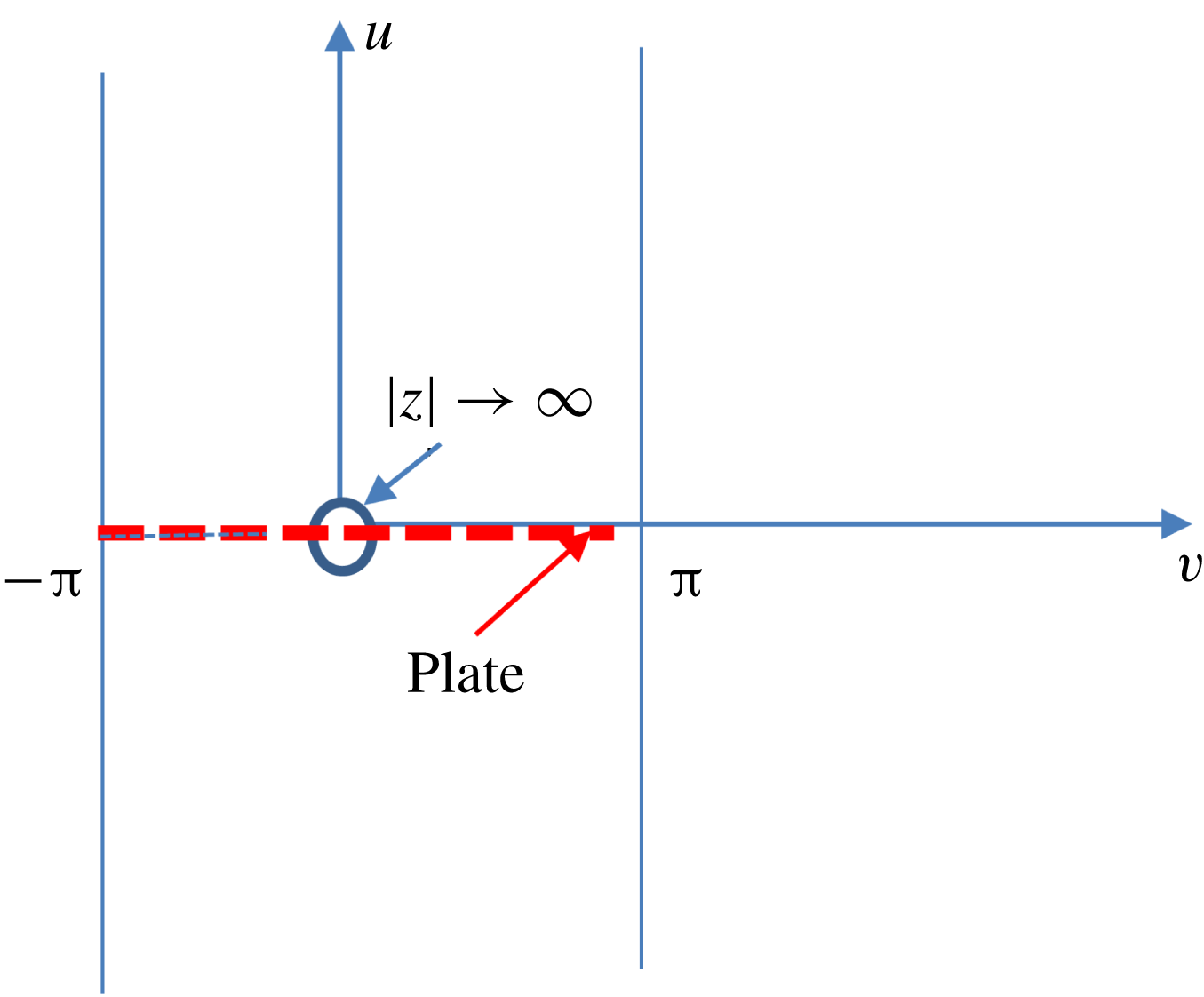
Appendix B. Modelling of physically realizable source spectra
The cross-correlation
 $$\begin{eqnarray}\displaystyle \unicode[STIX]{x1D6EC}(\,\boldsymbol{y}_{T},\tilde{\boldsymbol{y}}_{T}\boldsymbol{ : }\tilde{\unicode[STIX]{x1D70F}}) & \equiv & \displaystyle \langle \boldsymbol{{\mathcal{U}}}_{\bot }(\unicode[STIX]{x1D70F}-y_{1}/U(\,\boldsymbol{y}_{T}),\boldsymbol{y}_{T})\boldsymbol{{\mathcal{U}}}_{\bot }(\unicode[STIX]{x1D70F}-{\tilde{y}}_{1}/U(\tilde{\boldsymbol{y}}_{T})+\tilde{\unicode[STIX]{x1D70F}},\tilde{\boldsymbol{y}}_{T})\rangle \nonumber\\ \displaystyle & = & \displaystyle \langle \boldsymbol{{\mathcal{U}}}_{\bot }(\unicode[STIX]{x1D70F},\boldsymbol{y}_{T})\boldsymbol{{\mathcal{U}}}_{\bot }(\unicode[STIX]{x1D70F}+\tilde{\unicode[STIX]{x1D70F}}-[{\tilde{y}}_{1}/U(\tilde{\boldsymbol{y}}_{T})-y_{1}/U(\,\boldsymbol{y}_{T})],\tilde{\boldsymbol{y}}_{T})\rangle\end{eqnarray}$$
of
 $\boldsymbol{{\mathcal{U}}}_{\bot }(\unicode[STIX]{x1D70F}-y_{1}/U(\,\boldsymbol{y}_{T}),\boldsymbol{y}_{T})$
will exist and be independent of
 $\unicode[STIX]{x1D70F}$
when
 $\boldsymbol{{\mathcal{U}}}_{\bot }$
is a stationary function of
 $\unicode[STIX]{x1D70F}$
and hence also of
 $\unicode[STIX]{x1D70F}-y_{1}/U(\,\boldsymbol{y}_{T})$
(Wiener Reference Wiener1938). It therefore follows that
 $$\begin{eqnarray}\displaystyle & & \displaystyle (2\unicode[STIX]{x03C0})\lim _{T\rightarrow \infty }\frac{\overline{\boldsymbol{{\mathcal{U}}}}_{\bot }(\,\boldsymbol{y}_{T};\unicode[STIX]{x1D714},T)[\overline{\boldsymbol{{\mathcal{U}}}}_{\bot }(\tilde{\boldsymbol{y}}_{T};\unicode[STIX]{x1D714},T)]^{\ast }}{2T}\nonumber\\ \displaystyle & & \displaystyle \quad =\frac{1}{2\unicode[STIX]{x03C0}}\int _{-\infty }^{\infty }\exp \text{i}\unicode[STIX]{x1D714}(\tilde{\unicode[STIX]{x1D70F}}-[{\tilde{y}}_{1}/U(\tilde{\boldsymbol{y}}_{T})-y_{1}/U(\,\boldsymbol{y}_{T})])\unicode[STIX]{x1D6EC}(\,\boldsymbol{y}_{T},\tilde{\boldsymbol{y}}_{T}\boldsymbol{ : }\tilde{\unicode[STIX]{x1D70F}})\,\text{d}\tilde{\unicode[STIX]{x1D70F}}\end{eqnarray}$$
so that the cross-correlation
 $\unicode[STIX]{x1D6EC}(\,\boldsymbol{y}_{T},\tilde{\boldsymbol{y}}_{T}\boldsymbol{ : }\tilde{\unicode[STIX]{x1D70F}})$
of the upstream normal gradient-wise velocity coefficient needs to be specified before the source spectrum (4.21), and therefore the pressure spectrum (4.19), can actually be calculated. We are unaware of any actual measurements of this quantity, but it is well known that the transverse velocity correlation
 $\langle v_{\bot }^{\prime }(\,\boldsymbol{y},\unicode[STIX]{x1D70F})v_{\bot }^{\prime }({\tilde{y}}_{1},y_{2},{\tilde{y}}_{3},\unicode[STIX]{x1D70F}+\tilde{\unicode[STIX]{x1D70F}})\rangle /U(\,\boldsymbol{y}_{T})U(y_{2},{\tilde{y}}_{3})$
, which has been extensively measured, can be well represented by the exponential form
 $$\begin{eqnarray}\displaystyle & & \displaystyle \frac{\langle v_{\bot }^{\prime }(\,\boldsymbol{y},\unicode[STIX]{x1D70F})v_{\bot }^{\prime }({\tilde{y}}_{1},y_{2},{\tilde{y}}_{3},\unicode[STIX]{x1D70F}+\tilde{\unicode[STIX]{x1D70F}})\rangle }{U(\,\boldsymbol{y}_{T})U(y_{2},{\tilde{y}}_{3})}\nonumber\\ \displaystyle & & \displaystyle \quad =A(\,\boldsymbol{y}_{T})\exp -\sqrt{\{\tilde{\unicode[STIX]{x1D70F}}-[({\tilde{y}}_{1}-y_{1})/U_{c}]\}^{2}/\unicode[STIX]{x1D70F}_{0}^{2}+[(y_{3}-{\tilde{y}}_{3})/l_{3}]^{2}},\end{eqnarray}$$
where
 $l_{3}$
is a constant and
 $U_{c}$
denotes an empirically determined constant convection velocity. This is consistent with Taylor’s hypothesis (Taylor Reference Taylor1938) which assumes that the changes in
 $v_{\bot }^{\prime }$
at a fixed point are due to an unchanging pattern of turbulent motion over that point and can be formulated as
 $v^{\prime }(y_{1},\unicode[STIX]{x1D70F})=v^{\prime }(y_{1}-U_{c}\tilde{\unicode[STIX]{x1D70F}},\unicode[STIX]{x1D70F}+\tilde{\unicode[STIX]{x1D70F}})$
(Townsend Reference Townsend1976). Dennis & Nickels (Reference Dennis and Nickels2008) show that the optimal approximation is obtained when
 $U_{c}$
is set equal to the local mean velocity
 $U(\,\boldsymbol{y})$
(which is equal to
 $U(\,\boldsymbol{y}_{T})$
for transversely sheared mean flows). But Taylor’s hypothesis is an approximation which, as shown by Lin (Reference Lin1953) is only valid when the turbulence level is low, viscous effects are negligible and the mean shear is small. The first two conditions are also required for the validity of RDT but the third is definitely not.
The important point is that (B 3) is consistent with the requirements of transversely sheared mean-flow RDT when
 $U_{c}$
is set equal to
 $U(y_{2})$
. But this consistency also requires (see (B 1)) that the fully three-dimensional correlation
 $\langle v_{\bot }^{\prime }(\,\boldsymbol{y},t)v_{\bot }^{\prime }(\tilde{\boldsymbol{y}},t+\tilde{\unicode[STIX]{x1D70F}})\rangle /U(\,\boldsymbol{y}_{T})U(\tilde{\boldsymbol{y}}_{T})$
be represented by the exponential form
 $A(\,\boldsymbol{y}_{T},\tilde{\boldsymbol{y}}_{T})\exp -\sqrt{[f(\unicode[STIX]{x1D702}_{2}/l_{2},\unicode[STIX]{x1D702}_{3}/l_{3})]^{2}+\{\tilde{\unicode[STIX]{x1D70F}}-[{\tilde{y}}_{1}/U(\tilde{u} )-y_{1}/U(u)]\}^{2}/\unicode[STIX]{x1D70F}_{0}^{2}}$
, where
 $\unicode[STIX]{x1D70F}_{0},l_{2},l_{3}$
are constants,
 $$\begin{eqnarray}\unicode[STIX]{x1D702}_{2}\equiv u-\tilde{u} ,\quad \unicode[STIX]{x1D702}_{3}\equiv v-\tilde{v}\end{eqnarray}$$
and
 $A(\,\boldsymbol{y}_{T},\tilde{\boldsymbol{y}}_{T}),f(\unicode[STIX]{x1D702}_{2}/l_{2},\unicode[STIX]{x1D702}_{3}/l_{3})$
are, as yet, unspecified functions of the indicated arguments, rather than by the commonly used form
 $A(\,\boldsymbol{y}_{T})\exp -\sqrt{[f(\unicode[STIX]{x1D702}_{2}/l_{2},\unicode[STIX]{x1D702}_{3}/l_{3})]^{2}+\{\tilde{\unicode[STIX]{x1D70F}}-[({\tilde{y}}_{1}-y_{1})/U_{c}]\}^{2}/\unicode[STIX]{x1D70F}_{0}^{2}}$
– a result that would certainly be worth checking experimentally.
It therefore seems appropriate to represent
 $\unicode[STIX]{x1D6EC}(\,\boldsymbol{y}_{T},\tilde{\boldsymbol{y}}_{T}\boldsymbol{ : }\tilde{\unicode[STIX]{x1D70F}})=\lim _{y_{1},{\tilde{y}}_{1}\rightarrow -\infty }(y_{1}{\tilde{y}}_{1})^{2}\langle u_{\bot }(y_{1},\boldsymbol{y}_{T},t)u_{\bot }({\tilde{y}}_{1},\tilde{\boldsymbol{y}}_{T},t+\tilde{\unicode[STIX]{x1D70F}})\rangle =\lim _{y_{1},{\tilde{y}}_{1}\rightarrow -\infty }(y_{1}{\tilde{y}}_{1})^{2}\langle \unicode[STIX]{x1D70C}v_{\bot }^{\prime }(y_{1},\boldsymbol{y}_{T},t)\unicode[STIX]{x1D70C}v_{\bot }^{\prime }({\tilde{y}}_{1},\tilde{\boldsymbol{y}}_{T},t+\tilde{\unicode[STIX]{x1D70F}})\rangle$
by
 $$\begin{eqnarray}\displaystyle & & \displaystyle \unicode[STIX]{x1D6EC}(\,\boldsymbol{y}_{T},\tilde{\boldsymbol{y}}_{T}\boldsymbol{ : }\tilde{\unicode[STIX]{x1D70F}})=A(\,\boldsymbol{y}_{T},\tilde{\boldsymbol{y}}_{T})l_{2}^{4}\unicode[STIX]{x1D70C}(\,\boldsymbol{y}_{T})U(\,\boldsymbol{y}_{T})\unicode[STIX]{x1D70C}(\tilde{\boldsymbol{y}}_{T})U(\tilde{\boldsymbol{y}}_{T})\nonumber\\ \displaystyle & & \displaystyle \quad \times \,\exp -\sqrt{[f(\unicode[STIX]{x1D702}_{2}/l_{2},\unicode[STIX]{x1D702}_{3}/l_{3})]^{2}+\{\tilde{\unicode[STIX]{x1D70F}}-[{\tilde{y}}_{1}/U(\tilde{u} )-y_{1}/U(u)]\}^{2}/\unicode[STIX]{x1D70F}_{0}^{2}},\end{eqnarray}$$
where the amplitude
 $A(\,\boldsymbol{y}_{T},\tilde{\boldsymbol{y}}_{T})$
is expected to vanish as
 $\boldsymbol{y}_{T},\tilde{\boldsymbol{y}}_{T}\rightarrow 0,\infty$
.
And since
 $\unicode[STIX]{x1D70C}c^{2}$
is constant in transversely sheared flows, inserting this into (B 2), inserting the result into (4.21) and using (27) of Leib & Goldstein (Reference Leib and Goldstein2011) shows that (4.22) provides an appropriate model for the source function
 $S$
(Campbell & Foster Reference Campbell and Foster1948, p. 111 equation no. 867).
Appendix C. The gust component of the low-frequency Green’s function
The spanwise Fourier transform
 $$\begin{eqnarray}\tilde{G}^{(0)}(y_{2}\mid x_{2}:\unicode[STIX]{x1D714},k_{1},k_{3})\equiv \frac{1}{2\unicode[STIX]{x03C0}}\int _{-\infty }^{\infty }\text{e}^{\text{i}(y_{3}-x_{3})k_{3}}\overline{\overline{G}}\text{}^{(0)}(\,\boldsymbol{y}_{T}\mid \boldsymbol{x}_{T};k_{1},\unicode[STIX]{x1D714})\,\text{d}x_{3}\end{eqnarray}$$
of the gust component
 $\overline{\overline{G}}\text{}^{(0)}(\,\boldsymbol{y}_{T}\mid \boldsymbol{x}_{T};k_{1},\unicode[STIX]{x1D714})$
of the streamwise Fourier transform of the reduced Green’s function
 $\overline{\overline{G}}(\,\boldsymbol{y}_{T}\mid \boldsymbol{x};k_{1},\unicode[STIX]{x1D714})$
is expected to be independent of
 $y_{3}$
and therefore determined by
 $$\begin{eqnarray}\left[\frac{\text{d}^{2}}{\text{d}y_{2}^{2}}+(k_{\infty }^{2}-k_{1}^{2}-k_{3}^{2})\right]\tilde{G}^{(0)}(y_{2}\mid x_{2}:\unicode[STIX]{x1D714},k_{1},k_{3})=\frac{k_{\infty }^{2}}{(2\unicode[STIX]{x03C0})^{3}}\unicode[STIX]{x1D6FF}(y_{2}-x_{2})\end{eqnarray}$$
in the outer region where
 $\sqrt{k_{\infty }^{2}-k_{1}^{2}}y_{T},\sqrt{k_{\infty }^{2}-k_{1}^{2}}x_{T}=O(1)$
when
 $\overline{\overline{G}}\text{}^{(0)}(\,\boldsymbol{y}_{T}\mid \boldsymbol{x}_{T};k_{1},\unicode[STIX]{x1D714})$
depends on
 $x_{3},y_{3}$
only in the combination
 $x_{3}-y_{3}$
(which we will show to be the case in the low-frequency limit) and is therefore given by Goldstein (Reference Goldstein1976, p. 282)
 $$\begin{eqnarray}\tilde{G}^{(0)}(y_{2}\mid x_{2}:\unicode[STIX]{x1D714},k_{1},k_{3})=H(y_{2}x_{2})\frac{\text{e}^{-\sqrt{k_{1}^{2}+k_{3}^{2}-k_{\infty }^{2}}|x_{2}|}k_{\infty }^{2}w_{2}(y_{2},k_{3},k_{1})}{\unicode[STIX]{x1D6E5}(k_{1},k_{3})}\end{eqnarray}$$
for
 $|x_{2}|>|y_{2}|$
, where
 $H$
denotes the Heaviside function
 $$\begin{eqnarray}w_{2}(y_{2},k_{3},k_{1})=\text{e}^{-\sqrt{k_{1}^{2}+k_{3}^{2}-k_{\infty }^{2}}|y_{2}|}+b\text{e}^{\sqrt{k_{1}^{2}+k_{3}^{2}-k_{\infty }^{2}}|y_{2}|},\end{eqnarray}$$
 $b$
is an
 $O(1)$
constant and it follows from Abel’s theorem that
 $$\begin{eqnarray}\unicode[STIX]{x1D6E5}(k_{1})=-2(2\unicode[STIX]{x03C0})^{3}b\sqrt{k_{1}^{2}+k_{3}^{2}-k_{\infty }^{2}}.\end{eqnarray}$$
For simplicity, we only consider the symmetric case (which is usually the case of principal interest). The outer solution
 $\overline{\overline{\overline{G}}}\text{}^{(0)}(y_{2},y_{3}\mid x_{2}:\unicode[STIX]{x1D714},k_{1},k_{3})+\overline{\overline{\overline{G}}}\text{}^{(0)}(y_{2},y_{3}\mid x_{2}:\unicode[STIX]{x1D714},k_{1},-k_{3})$
(where
 $\overline{\overline{\overline{G}}}\text{}^{(0)}(y_{2},y_{3}\mid x_{2}:\unicode[STIX]{x1D714},k_{1},k_{3})\equiv \overline{\overline{\overline{G}}}\text{}^{(0)}(u(y_{2},y_{3}),v(y_{2},y_{3})\mid x_{2}:\unicode[STIX]{x1D714},k_{1},k_{3})$
see (5.8)) must then behave like
 $$\begin{eqnarray}\displaystyle & & \displaystyle \overline{\overline{\overline{G}}}\text{}^{(0)}(y_{2},y_{3}\mid x_{2}:\unicode[STIX]{x1D714},k_{1},k_{3})+\overline{\overline{\overline{G}}}\text{}^{(0)}(y_{2},y_{3}\mid x_{2}:\unicode[STIX]{x1D714},k_{1},-k_{3})=\text{e}^{-\text{i}k_{3}y_{3}}\tilde{G}^{(0)}(y_{2}\mid x_{2}:\unicode[STIX]{x1D714},k_{1},k_{3})\nonumber\\ \displaystyle & & \displaystyle \qquad +\,\text{e}^{\text{i}k_{3}y_{3}}\tilde{G}^{(0)}(y_{2}\mid x_{2}:\unicode[STIX]{x1D714},k_{1},-k_{3})=(\text{e}^{-\text{i}k_{3}y_{3}}+\text{e}^{\text{i}k_{3}y_{3}})\tilde{G}^{(0)}(y_{2}\mid x_{2}:\unicode[STIX]{x1D714},k_{1},k_{3})\nonumber\\ \displaystyle & & \displaystyle \quad =2\tilde{G}^{(0)}(y_{2}\mid x_{2}:\unicode[STIX]{x1D714},k_{1},k_{3})+O(k_{3}y_{3})^{2},\quad \text{as }k_{3}y_{3}\rightarrow 0\end{eqnarray}$$
 $$\begin{eqnarray}\tilde{G}^{(0)}(y_{2}\mid x_{2}:\unicode[STIX]{x1D714},k_{1},k_{3})=\tilde{G}^{(0)}(y_{2}\mid x_{2}:\unicode[STIX]{x1D714},k_{1},-k_{3}).\end{eqnarray}$$
And it, therefore, follows that the inner limit of the outer symmetric part of the Fourier-transformed Green’s function is
 $$\begin{eqnarray}\displaystyle & & \displaystyle \overline{\overline{\overline{G}}}\text{}^{(0)}(y_{2},y_{3}\mid x_{2}:\unicode[STIX]{x1D714},k_{1},k_{3})+\overline{\overline{\overline{G}}}\text{}^{(0)}(y_{2},y_{3}\mid x_{2}:\unicode[STIX]{x1D714},k_{1},-k_{3})\nonumber\\ \displaystyle & & \displaystyle \quad \rightarrow \,\frac{-k_{\infty }^{2}\text{e}^{-\sqrt{k_{1}^{2}+k_{3}^{2}-k_{\infty }^{2}}|x_{2}|}}{(2\unicode[STIX]{x03C0})^{3}b\sqrt{k_{1}^{2}+k_{3}^{2}-k_{\infty }^{2}}}H(y_{2}x_{2})\nonumber\\ \displaystyle & & \displaystyle \quad \times \,\left\{\left[(1+b)+(b-1)\sqrt{k_{1}^{2}+k_{3}^{2}-k_{\infty }^{2}}|y_{2}|\right]+O(y_{2}^{2}(k_{1}^{2}+k_{3}^{2}-k_{\infty }^{2}))\right\},\nonumber\\ \displaystyle & & \displaystyle \qquad \quad \text{as }y_{2}\sqrt{k_{1}^{2}+k_{3}^{2}-k_{\infty }^{2}}\rightarrow 0.\end{eqnarray}$$
This result will satisfy the wall boundary condition in the outer region where
 $k_{3}y_{3}=O(1)$
if we set
 $b=1$
. When
 $\boldsymbol{y}_{T}$
is in the inner region and
 $\boldsymbol{x}_{T}$
is in the outer region (5.11) and (5.12) possess a solution of the form
 $$\begin{eqnarray}\displaystyle & & \displaystyle {\textstyle \frac{1}{2}}[\overline{\overline{\overline{G}}}\text{}^{(0)}(u,v\mid x_{2}:\unicode[STIX]{x1D714},k_{1},k_{3})+\overline{\overline{\overline{G}}}\text{}^{(0)}(u,v\mid x_{2}:\unicode[STIX]{x1D714},k_{1},-k_{3})]\nonumber\\ \displaystyle & & \displaystyle \quad =a_{0}^{\pm }(x_{2},k_{1},k_{3},\unicode[STIX]{x1D714})(1+O(k_{\infty }^{2}))\quad \text{for }x_{2}\gtrless 0,\end{eqnarray}$$
which is symmetric in
 $k_{3}$
satisfies the spanwise transform of the zero derivative wall boundary condition and will match onto the outer solution (C 6) to within an error of
 $O(k_{1}^{2}+k_{3}^{2}-k_{\infty }^{2})$
in the overlap domain where
 $u,v\rightarrow 0,y_{2}\sqrt{k_{1}^{2}+k_{3}^{2}-k_{\infty }^{2}},k_{3}y_{3}\rightarrow 0$
if we set
 $b=1$
and
 $$\begin{eqnarray}a_{0}^{\pm }(x_{2},k_{1},k_{3},\unicode[STIX]{x1D714})=\frac{-k_{\infty }^{2}\text{e}^{\mp \sqrt{k_{1}^{2}+k_{3}^{2}-k_{\infty }^{2}}x_{2}}}{(2\unicode[STIX]{x03C0})^{3}\sqrt{k_{1}^{2}+k_{3}^{2}-k_{\infty }^{2}}}H(x_{2}y_{2}).\end{eqnarray}$$
The lowest-order inner solution for the Fourier-transformed Green’s function that satisfies the wall boundary condition (2.8) for all values of
 $y_{3}$
is therefore given by (5.20).
Appendix D. The scattered component of the low-frequency Fourier-transformed Green’s function
Equations (5.7), (5.8), (6.1) and (5.15)–(5.17) show that the inner solution for the Fourier transform
 $\overline{\overline{\overline{G}}}\text{}_{+}^{(s)}(u,v\mid x_{1},x_{2}:\unicode[STIX]{x1D714},k_{1},k_{3})$
of the scattered component of the Green’s function must be of the form
 $$\begin{eqnarray}\displaystyle \overline{\overline{\overline{G}}}\text{}_{+}^{(s)}(u,v\mid x_{1},x_{2};k_{1},k_{3},\unicode[STIX]{x1D714}) & = & \displaystyle \mathop{\sum }_{n=-\infty }^{\infty }\text{e}^{\text{i}nv}\overline{\overline{\boldsymbol{{\mathcal{G}}}}}\text{}_{n}^{(s)}(u\mid x_{1},x_{2}:\unicode[STIX]{x1D714},k_{1},k_{3})\nonumber\\ \displaystyle & = & \displaystyle \mathop{\sum }_{n=-\infty }^{\infty }\text{e}^{\text{i}nv}A_{n}^{(s)}(x_{1},x_{2};k_{1},k_{3},\unicode[STIX]{x1D714})\hat{P}_{n}^{\gtrless }(u:\unicode[STIX]{x1D714},k_{1}),\end{eqnarray}$$
where
 $$\begin{eqnarray}\hat{P}_{0}^{\gtrless }(u)=c_{0}^{\gtrless }+c_{1}^{\gtrless }\int _{0}^{u}\frac{[M(u)k_{1}/k_{\infty }-1]^{2}}{c^{2}(u)}\,\text{d}u,\end{eqnarray}$$
and
 $\hat{P}_{n}^{\gtrless }(u:\unicode[STIX]{x1D714},k_{1})$
for
 $n=\pm 1,\pm 2,\ldots ,$
denote specific solutions of (5.16) and (5.17) that behave like
 $$\begin{eqnarray}\hat{P}_{n}^{\pm }(u:\unicode[STIX]{x1D714},k_{1},k_{3})\rightarrow \text{e}^{\pm |n|u}\quad \text{as }u\rightarrow 0.\end{eqnarray}$$
And in order to ensure that
 $\overline{\overline{\overline{G}}}\text{}^{(s)}$
behaves like the Fourier transform of the zero-mean-flow flat plate Green’s function in the outer region where
 $k_{3}y_{3},y_{2}=O(1)$
, we require that the inner solution (D 1) match onto the outgoing wave outer solution
 $$\begin{eqnarray}\displaystyle \overline{\overline{\overline{G}}}\text{}_{+}^{(s)}(y_{2},y_{3}\mid x_{1},x_{2}:\unicode[STIX]{x1D714},k_{1},k_{3}) & = & \displaystyle A_{\gtrless }^{(s)}(x_{1},x_{2}\mid k_{1},k_{3},k_{\infty })\hat{P}^{\gtrless }(\,\boldsymbol{y}_{T}\boldsymbol{ : }\unicode[STIX]{x1D714},k_{1},k_{3})\nonumber\\ \displaystyle & & \displaystyle +\,O(k_{1}^{2}+k_{3}^{2}-k_{\infty }^{2}),\quad \text{for }y_{2}\gtrless 0,\end{eqnarray}$$
where
 $\overline{\overline{\overline{G}}}\text{}_{+}^{(s)}(y_{2},y_{3}\mid x_{1},x_{2}:\unicode[STIX]{x1D714},k_{1},k_{3})\equiv \overline{\overline{\overline{G}}}\text{}_{+}^{(s)}(u(y_{2},y_{3}),v(y_{2},y_{3})\mid x_{1},x_{2},\unicode[STIX]{x1D714},k_{1},k_{3})$
and
 $$\begin{eqnarray}\hat{P}^{\gtrless }(\,\boldsymbol{y}_{T}\boldsymbol{ : }\unicode[STIX]{x1D714},k_{1},k_{3})={\textstyle \frac{1}{2}}\exp \left(\mp \sqrt{k_{1}^{2}+k_{3}^{2}-k_{\infty }^{2}}y_{2}\right)[\exp (\text{i}k_{3}y_{3})+\exp (-\text{i}k_{3}y_{3})]+o(k_{\infty })\end{eqnarray}$$
is an outgoing wave solution of the Helmholtz equation (see (5.19))
 $$\begin{eqnarray}\boldsymbol{{\mathcal{L}}}\hat{P}^{\gtrless }(\,\boldsymbol{y}_{T}\boldsymbol{ : }\unicode[STIX]{x1D714},k_{1},k_{3})=0\end{eqnarray}$$
in the outer region where
 $\sqrt{k_{1}^{2}+k_{3}^{2}-k_{\infty }^{2}}y_{2},k_{3}y_{3}=O(1)$
. The
 $\mp$
sign in the exponent comes from the requirement that this solution have outgoing wave behaviour as
 $y_{2}\rightarrow \pm \infty$
.
An appropriate choice for
 $\hat{P}^{\gtrless }(\,\boldsymbol{y}_{T}\boldsymbol{ : }\unicode[STIX]{x1D714},k_{1})$
is
 $$\begin{eqnarray}\displaystyle & & \displaystyle \hat{P}^{\gtrless }(\,\boldsymbol{y}_{T}\boldsymbol{ : }\unicode[STIX]{x1D714},k_{1},k_{3})={\textstyle \frac{1}{2}}\exp \left(\mp \sqrt{k_{1}^{2}+k_{3}^{2}-k_{\infty }^{2}}y_{2}\right)[\exp (\text{i}k_{3}y_{3})+\exp (-\text{i}k_{3}y_{3})]\nonumber\\ \displaystyle & & \displaystyle \quad +\,a_{\gtrless }(k_{1},k_{3},k_{\infty })\unicode[STIX]{x03C0}\sqrt{k_{\infty }^{2}-k_{1}^{2}}\nonumber\\ \displaystyle & & \displaystyle \quad \times \,\left[\text{e}^{\pm \text{i}\unicode[STIX]{x1D711}}H_{1}^{(1)}\left(y_{T}\sqrt{k_{\infty }^{2}-k_{1}^{2}}\right)+\text{e}^{\mp \text{i}\unicode[STIX]{x1D711}}H_{-1}^{(1)}\left(y_{T}\sqrt{k_{\infty }^{2}-k_{1}^{2}}\right)\right]\quad y_{2}\gtrless 0,\end{eqnarray}$$
where
 $H_{\unicode[STIX]{x1D708}}^{(1)}$
denotes the Bessel function of the first kind and
 $a(k_{1},k_{3},k_{\infty })$
is a function of the indicated arguments.
It now follows from (D 2), (A 2) and #9.1.8 on p. 360 of Abramowitz & Stegun (1964) that the inner limit of the outer solution (D 5) is
 $$\begin{eqnarray}\displaystyle & & \displaystyle \hat{P}^{\gtrless }(u:\unicode[STIX]{x1D714},k_{1},k_{3})\rightarrow 1\mp \sqrt{k_{1}^{2}+k_{3}^{2}-k_{\infty }^{2}}y_{2}-a_{\gtrless }(\text{e}^{\pm \text{i}\unicode[STIX]{x1D711}}-\text{e}^{\mp \text{i}\unicode[STIX]{x1D711}})\text{i}\frac{2}{y_{T}}+O(k_{1}^{2}+k_{3}^{2}-k_{\infty }^{2})\nonumber\\ \displaystyle & & \displaystyle \quad \rightarrow \,1\mp \sqrt{k_{1}^{2}+k_{3}^{2}-k_{\infty }^{2}}y_{2}\pm 2a_{\gtrless }Re\,\frac{2\text{i}}{z}+O(k_{1}^{2}+k_{3}^{2}-k_{\infty }^{2})\nonumber\\ \displaystyle & & \displaystyle \quad =1\mp \sqrt{k_{1}^{2}+k_{3}^{2}-k_{\infty }^{2}}Re\,\left(\frac{\text{e}^{W}+1}{1-\text{e}^{W}}\right)\nonumber\\ \displaystyle & & \displaystyle \qquad \mp \,2a_{\gtrless }Re\,W+O(k_{1}^{2}+k_{3}^{2}-k_{\infty }^{2})\rightarrow 1-\sqrt{k_{1}^{2}+k_{3}^{2}-k_{\infty }^{2}}\nonumber\\ \displaystyle & & \displaystyle \qquad \times \,\left(1+2Re\,\mathop{\sum }_{n=1}^{\infty }\text{e}^{\pm nW}\right)\mp 2a_{\gtrless }u+O(k_{1}^{2}+k_{3}^{2}-k_{\infty }^{2})\rightarrow 1\nonumber\\ \displaystyle & & \displaystyle \qquad -\,\sqrt{k_{1}^{2}+k_{3}^{2}-k_{\infty }^{2}}\mathop{\sum }_{n=-\infty }^{\infty }\text{e}^{\text{i}nv\pm |n|u}\mp 2a_{\gtrless }u+O(k_{1}^{2}+k_{3}^{2}-k_{\infty }^{2}),\end{eqnarray}$$
as
 $\sqrt{k_{1}^{2}+k_{3}^{2}-k_{\infty }^{2}}y_{2},k_{3}y_{3}\rightarrow 0$
. And since it follows from (D 1)–(D 3) that the inner solution behaves like
 $$\begin{eqnarray}\overline{\overline{\overline{G}}}\text{}_{+}^{(s)}(u,v\mid x_{1},x_{2};k_{1},k_{3},\unicode[STIX]{x1D714})\rightarrow c_{0}^{\gtrless }+c_{1}^{\gtrless }u+\mathop{\sum }_{n=-\infty }^{\infty }\text{e}^{\text{i}nv}\tilde{A}_{n}^{(s)}(k_{1},k_{3},\unicode[STIX]{x1D714})\text{e}^{\pm |n|u}\end{eqnarray}$$
as
 $u,v\rightarrow 0$
, the inner and outer expansions will only match if
 $$\begin{eqnarray}c_{0}^{\gtrless }=1,c_{1}^{\gtrless }=\mp 2a_{\gtrless },\quad \tilde{A}_{n}^{(s)}=-\sqrt{k_{1}^{2}+k_{3}^{2}-k_{\infty }^{2}},\quad n=0,\pm 1,\pm 2.\end{eqnarray}$$
It then follows from (D 1) and (D 2) that the Fourier transform of the scattered component of the Green’s function is of the form (5.22).