Introduction
As an emerging wireless power transmission technology, microwave power transmission (MPT) and energy harvesting (EH) have attracted significant research attention due to their numerous advantages [Reference Wu and Liu1, Reference Du, Cheng, Wu and Gu2]. These technologies offer a promising solution to the critical limitation of battery lifespan in wireless sensor networks (WSNs) [Reference He, Liao, He, Yan and Liu3, Reference Shinohara4], thereby significantly improving power availability and enabling the broader deployment of WSNs across various application scenarios [Reference He, Zhou, He, Feng and Liu5–Reference Paolini, Battistini, Di Renzo, Fazzini, Tiberi, Trovarello, Masotti and Costanzo7].
Within MPT and EH systems, two persistent challenges are maximizing the capture of incident electromagnetic energy and improving the radio frequency to direct current (RF-to-DC) conversion efficiency [Reference Liu, Tan, Zhang and He8, Reference He, Liao, He, Yan and Liu9]. A significant challenge in achieving high-efficiency wideband rectification is the nonlinear and frequency-dependent input impedance of the rectifying diode. This nonlinearity complicates the impedance matching process across a broad frequency range. To address this challenge, non-uniform transmission lines have been effectively employed to realize broadband impedance matching, enabling rectifiers to maintain high conversion efficiency over extended bandwidths [Reference Bolos, Belo and Georgiadis10, Reference Wu11]. Additionally, the integration of harmonic termination techniques has been shown to improve bandwidth without increasing circuit dimensions [Reference He, Lin, Wu, Li and Liu12, Reference Bui, Nguyen and Seo13]. In terms of novel impedance compression techniques, the primary method to achieve small size and high efficiency is to compress the variation range of the rectifier’s input impedance [Reference Bo, Ou and Zhang14, Reference Ming Wang, Fei Bo, Ou and Yin Zhang15]. To further enhance rectifier performance, several advanced strategies have been investigated. These include frequency-selective multi-branch architectures [Reference Wu, Huang, Zhou and Liu16–Reference Liu, Ou, Zhang, Gui, Zhang and Li18], complementary resonant structures for dynamic frequency-dependent switching [Reference Lu, Song and Huang19], simplified real-frequency design techniques [Reference Lin, Zhang, Du and Lin20], and complex impedance-matching networks tailored for broadband operation [Reference Liu, Huang, Wang, Hou and Zhang21, Reference Cheng, Du, Wu and Gu22]. These approaches have contributed to the continued advancement of high-efficiency, wideband rectifier designs for next-generation wireless power systems.
An earlier version of this paper was presented at EuMW 2025 and was published in its Proceedings [Reference He, Song, He, Yan and Liu23]. Compared with our previous work [Reference He, Zhou, Ren, Yan, He and Liu24], which primarily focuses on efficiency enhancement, this paper analyzes the matching mechanism of the structure and, based on its operating characteristics, identifies the most suitable broadband matching impedance conditions for ultra-wideband rectifier applications. Two different rectifier prototypes were fabricated and experimentally validated to demonstrate the effectiveness of the proposed matching impedance approach over an ultra-wide bandwidth. This work places greater emphasis on the impedance-matching capability of the matching network over an ultra-wide frequency range. By properly selecting the impedance space, the operating bandwidth is significantly extended.
Principle and design method
Analysis of the coupled matching structure
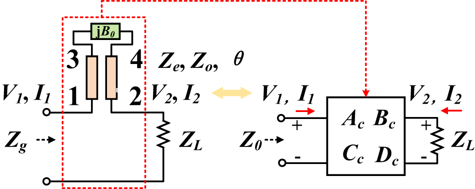
The schematic of the proposed coupled matching structure (CMS) is illustrated in Figure 1. The coupled transmission line has an electrical length of θ, with even- and odd-mode characteristic impedances denoted as Ze and Zo, respectively. A susceptive element with susceptance B 0 is connected between ports 3 and 4 of the coupled lines. The two-port network formed between ports 1 and 2 can be characterized using an ABCD matrix, which relates the source impedance Z g to the load impedance ZL. To facilitate theoretical analysis, the network is decomposed into even- and odd-mode excitation cases. The corresponding ABCD matrices for the even and odd modes are derived and denoted as [Reference Pozar25]:
 \begin{equation}\left[ {\begin{array}{*{20}{c}}
{{A_e}}&{{B_e}} \\
{{C_e}}&{{D_e}}
\end{array}} \right] = \left[ {\begin{array}{*{20}{c}}
{\cos \theta }&{j{Z_e}\sin \theta } \\
{j\sin \theta /{Z_e}}&{\cos \theta }
\end{array}} \right]\end{equation}
 \begin{equation}\left[ {\begin{array}{*{20}{c}}
{{A_o}}&{{B_o}} \\
{{C_o}}&{{D_o}}
\end{array}} \right] = \left[ {\begin{array}{*{20}{c}}
{\cos \theta - 2{B_0}{Z_o}\sin \theta }&{j{Z_o}\sin \theta } \\
{j\left( {\sin \theta /{Z_o} + 2{B_0}\cos \theta } \right)}&{\cos \theta }
\end{array}} \right]\end{equation}
The proposed coupled matching structure and its equivalent two-port network.

(1) Long description
Coupled matching structure with a transmission line between ports 1 and 2, characterized by even-mode impedance Ze, odd-mode impedance Zo and electrical length theta. A susceptance element with susceptance B subscript 0 is connected between ports 3 and 4. The source impedance Z subscript g is connected to port 1 and the load impedance Z subscript L is connected to port 2. The two-port network is represented by an ABCD matrix with parameters A subscript c, B subscript c, C subscript c and D subscript c, relating the input voltage V subscript 1 and current I subscript 1 to the output voltage V subscript 2 and current I subscript 2. The network facilitates impedance matching between the source and load.
The two-port coupled-line network matrix is formulated as
 \begin{equation}\left[ {\begin{array}{*{20}{c}}
{{A_c}}&{{B_c}} \\
{{C_c}}&{{D_c}}
\end{array}} \right] = \left[ {\begin{array}{*{20}{c}}
{\frac{{{A_e}{C_o} + {A_o}{C_e}}}{{{A_e}{C_o} - {A_o}{C_e}}}}&{\frac{{2{A_e}{A_o}}}{{{A_e}{C_o} - {A_o}{C_e}}}} \\
{\frac{{2{C_e}{C_o}}}{{{A_e}{C_o} - {A_o}{C_e}}}}&{\frac{{{A_e}{C_o} + {A_o}{C_e}}}{{{A_e}{C_o} - {A_o}{C_e}}}}
\end{array}} \right]\end{equation}
By analyzing the ABCD matrix, we obtain the voltage reflection coefficient as
 \begin{equation}{S_{11}} = \frac{{{A_c}{Z_{\text{L}}} + {B_c} - {C_c}{Z_g}{Z_{\text{L}}} - {D_c}{Z_g}}}{{{A_c}{Z_{\text{L}}} + {B_c} + {C_c}{Z_g}{Z_{\text{L}}} + {D_c}{Z_g}}}\end{equation}
where ZL = RL + jXL is the load impedance, and RL is greater than zero.
As an ideal impedance match, the condition S 11 = 0. Equation (4) is simplified as
 \begin{equation}{Z_e} = \left( {{M_1} + \sqrt {M_1^2 + {M_2}} } \right)\tan \theta \end{equation}
 \begin{equation}{B_0} = \frac{{{M_2}{{\tan }^2}\theta + {Z_e}{Z_o}}}{{2\left( {{Z_e}{Z_o} - {M_2}} \right){Z_o}\tan \theta }}\end{equation}
where  ${Z_{\text{g}}} = {R_S},\;{R_L} \ne {R_S}$ and
 \begin{equation}{M_1} = \frac{{{R_{\text{S}}}{X_{\text{L}}}}}{{{R_{\text{L}}} - {R_{\text{S}}}}}\end{equation}
 \begin{equation}{M_2} = \frac{{{R_{\text{S}}}{X_{\text{L}}}^2}}{{{R_{\text{L}}} - {R_{\text{S}}}}} + {R_{\text{S}}}{R_{\text{L}}}\end{equation}
Equations (5) to (8) indicate that the odd-mode impedance Zo and θ are two independent design variables, unaffected by the load impedance ZL or the source impedance Rs. This decoupling allows these parameters to be freely tuned, offering significant flexibility in the design of CMS for broadband rectifier applications. When the load impedance is symmetrically distributed along the real axis on the Smith chart, i.e., the load impedance ZL at the center frequency f 0 is set to ZL = RL, and the load impedance at the start frequency f 1 and the stop frequency f 2 are Zf 1 = RL − jXL 1 and Zf 2 = RL + jXL 1, respectively. By solving the equation for Zo and θ, CMS can successfully match the impedance at f 0, f 1, and f 2. At this point, the impedance across the entire frequency band is also matched to the microwave source impedance.
Based on this theoretical framework, the CMS can effectively transform arbitrary complex load impedances into the desired source impedance, enabling wideband impedance matching.
Design of the rectifier
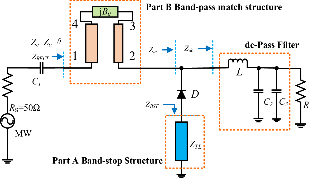
Figure 2 illustrates the schematic of the proposed wideband rectifier. Part A is a band-stop structure formed by a series λg/8 short-ended transmission line, while Part B represents the CMS. The input impedance of the λg/8 short-ended transmission line is
 \begin{equation}{Z_{{\text{BSF}}}} = j{Z_{{\text{TL}}}}\tan \left( {\frac{\pi }{4}\frac{f}{{{f_0}}}} \right) = \left\{ \begin{array}{*{20}{c}}
{j{Z_{{\text{TL}}}}\tan \left( {\frac{\pi }{4}\frac{f}{{{f_0}}}} \right)}&{0 \lt f \lt {f_0}} \\
{j{Z_{TL}}}&{f = {f_0}} \\
{j{Z_{{\text{TL}}}}\tan \left( {\frac{\pi }{4}\frac{f}{{{f_0}}}} \right)}&{{f_0} \lt f \lt 2{f_0}} \\
\infty &{f = 2{f_0}}
\end{array}\right.\end{equation}
where Z TL is the characteristic impedance of the transmission line.
Proposed wideband rectifier I with the CMS.

Figure 2 Long description
The circuit diagram features a wideband rectifier with distinct sections labeled as Part A and Part B. Part A is a band-stop structure with a series transmission line labeled Z subscript BSF. It includes a capacitor C subscript 1 connected to a microwave source MW with a source resistance R subscript S equals 50 ohm. The transmission line Z subscript TL is connected to a diode D. Part B is a band-pass match structure with components labeled 1, 2, 3 and 4 and an impedance jB subscript 0. The circuit continues with a dc-pass filter comprising an inductor L and capacitors C subscript 2 and C subscript 3, connected in parallel to a resistive load R. The connections are marked with impedances Z subscript RECT, Z subscript in and Z subscript dc. The circuit is grounded at multiple points, including the resistive load and capacitors C subscript 2 and C subscript 3.
The impedance Z BSF is inductive at f0, compensating for the diode’s capacitive reactance, i.e., Im(ZD) = −Z TL. It facilitates impedance matching at f 0. Z BSF is infinite at 2f 0, which helps to recycle the second harmonic at 2f 0 during rectification. Thus, the rectification efficiency is improved.
Zdc is the input impedance of the dc-pass filter, which provides an open circuit for all RF signals in the operating band. Zin is equal to the parallel of the diode branch and the dc-filter. Thus, Zdc is neglected. In this case, Zin becomes the equivalent load to the CMS, i.e., ZL = Zin.
Zin becomes the impedance of the diode in series with the band-stop structure as
 \begin{equation}{Z_{in}} = {Z_D} + {Z_{{\text{BSF}}}}\end{equation}
Thus, Zin is capacitive when f < f 0 and inductive when f 0 < f < 2f 0 from Equation (9).
We choose 2.45 GHz as the center frequency f0 in the wideband rectifier design. Due to the analysis of the band-stop structure, Zin is approximately located along a constant resistance circle on the Smith chart in the operating frequency band, as shown in Figure 3a. The band-stop structure compensates for the diode impedance at f 0 to become a resistance located at the real axis. Zin is above the real axis when f 0 < f < 2f 0 and below the real axis when f < f 0, distributed almost conjugately around the real axis in the Smith chart.
Therefore, the imaginary part of the impedance of the diode series with the band-stop structure at an input power level is
 \begin{equation}Im\left( {{Z_{in}}} \right){|_{f = {f_0}}} = Im\left( {{Z_D} + {Z_{{\text{BSF}}}}} \right){|_{f = {f_0}}}\end{equation}
The load impedance ZL at the center frequency f0 is set to ZL = RL. Then, the load impedance at the start frequency f 1 and the stop frequency f 2 is Zf 1 = RL—jXL 1 and Zf2 = RL + jXL 1, respectively.
Based on the analysis of the band-stop structure, the input impedance Zin is approximately distributed along a constant-resistance circle on the Smith chart over the operating frequency band, as shown in Figure 3a. Accordingly, the load impedance is defined as ZL = RL, while the input impedances at the center frequency f 0, start frequency f 1, and stop frequency f 2 are expressed as Zf 1 = RL − jXL 1 and Zf2 = RL + jXL 1, respectively.
For optimal rectifier operation, the input impedance must be matched to the system characteristic impedance, i.e., Z₀ = 50 Ω. Consequently, the source impedance is set to Z₀ = R s = 50 Ω. Substituting these conditions into Equations (8) and (9) yields Equations (13) and (14).
 \begin{equation}{M_1} = \frac{{{Z_0}{X_{\text{L}}}}}{{{R_{\text{L}}} - {Z_0}}}\end{equation}
 \begin{equation}{M_2} = \frac{{{Z_0}{X_{\text{L}}}^2}}{{{R_{\text{L}}} - {Z_0}}} + {Z_0}{R_{\text{L}}}\end{equation}
 \begin{align}
{Z_e} &= \left( { - {M_1}\left( {{f_1}} \right) + \sqrt {M_1^2\left( {{f_1}} \right) + {M_2}\left( {{f_1}} \right)} } \right)\tan \left( {{\theta _0}\frac{{{f_1}}}{{{f_0}}}} \right) \nonumber \\
\;\;\;\; &= \left( {M_1\left( {{f_2}} \right) + \sqrt {M_1^2\left( {{f_2}} \right) + {M_2}\left( {{f_2}} \right)} } \right)\tan \left( {{\theta _0}\frac{{{f_2}}}{{{f_0}}}} \right)
\end{align}
Since the even-mode impedance Ze exhibits minimal variation with frequency, it is possible to establish equations to determine the electrical length θ and achieve impedance matching at both f 1 and f 2. Notably, the load impedances at f 1 and f 2 are approximately complex conjugates, leading to identical values of M2, i.e., M 2(f 1) = M 2(f 2), while M 1 exhibits opposite signs, such that M 1(f 1) = −M 1(f 2). As shown in Equation (12), the electrical length at the center frequency, denoted as θ 0, is selected as the electrical length of the CMS. Through this approach, a value of θ 0 is derived that enables conjugate impedance matching simultaneously at the start and stop frequencies.
Further analysis reveals that the susceptive element in the CMS is an inductor L0. For a given inductance value, the susceptance B0(f 0) varies with frequency, where B0(f 0) and B0(f 2) correspond to the susceptance at the center frequency B0(f 0) and stop frequency f 2, respectively. As shown in Equations (13) and (14), by exploiting the frequency-dependent behavior of the inductor L0 to satisfy both B0(f 0) and B0(f 2), the characteristic impedance Zo can be derived, thereby enabling simultaneous impedance matching at f 0 and f 2. As a result, the CMS achieves effective impedance matching at all three critical frequency points: f 0, f 1, and f 2.
 \begin{equation}\left. {{B_0}\left( f \right)} \right|{f_0} = \frac{1}{{2\pi j{f_0}{L_0}}} = \frac{{{M_2}\left( {{f_0}} \right){{\tan }^2}\left( {{\theta _0}} \right) + {Z_e}{Z_o}}}{{2\left( {{Z_e}{Z_o} - {M_2}\left( {{f_0}} \right)} \right){Z_o}\tan \left( {{\theta _0}} \right)}}\end{equation}
 \begin{equation}{\left. {{B_0}\left( f \right)} \right|_{{f_2}}} = \frac{1}{{2\pi j{f_2}{L_0}}} = \frac{{{M_2}\left( {{f_2}} \right){{\tan }^2}\left( {{\theta _0}\frac{{{f_2}}}{{{f_0}}}} \right) + {Z_e}{Z_o}}}{{2\left( {{Z_e}{Z_o} - {M_2}\left( {{f_2}} \right)} \right){Z_o}\tan \left( {{\theta _0}\frac{{{f_2}}}{{{f_0}}}} \right)}}\end{equation}
Although achieving perfect impedance matching across the entire operating bandwidth is inherently challenging, matching at the three representative frequencies – start f 1, center f 0, and stop f 2 – provides a practical and effective design strategy. All parameters were subsequently fine-tuned using full-wave and circuit-level simulations to further optimize performance. As shown in Figure 3b, the rectifier input impedance remains close to 50 Ω across the operating band, confirming the effectiveness of the proposed impedance-matching approach.
Zin over 1.9–3.1 GHz at various input power levels. (b) ZRECT over 1.7–3.2 GHz at different input power levels.

Figure 3 Long description
Smith chart of input impedance locus versus frequency. The chart grid shows real-axis labels 0.2, 0.5, 1.0, 2.0 and 5.0 and imaginary-axis labels 0.2j, 0.5j, 1.0j, 2.0j and 5.0j, with matching negative imaginary labels. A legend lists four traces labeled 0 dBm, 5 dBm, 11 dBm and 15 dBm. Two frequency annotations are printed: 1.9 GHz and 3.1 GHz. Two oval callouts mark two locations on the plotted loci. The plotted loci for the four power levels form curved paths that stay within the Smith chart boundary and cluster around the region between the real-axis labels 1.0 and 5.0. Smith chart of rectifier impedance locus versus frequency. The chart grid shows real-axis labels 0.2, 0.5, 1.0, 2.0 and 5.0 and imaginary-axis labels 0.2j, 0.5j, 1.0j, 2.0j and 5.0j, with matching negative imaginary labels. A legend lists four traces labeled 0 dBm, 5 dBm, 11 dBm and 15 dBm. Two frequency annotations are printed: 1.7 GHz and 3.2 GHz. The text 1.0 is printed near the chart center. One trace includes multiple arrowheads along the curve and an additional arrow points toward the center region. The plotted loci for the four power levels form loops and arcs around the central region near the real-axis label 1.0, with the different power-level traces separated from each other along parts of the locus.
Design of the ultra-wideband rectifier
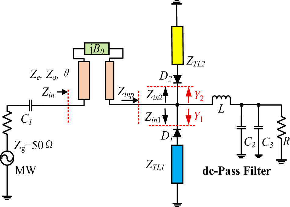
To further validate the proposed wideband rectifier approach, an ultra-wideband low-power rectifier is designed, as illustrated in Figure 4. This rectifier features a dual-diode configuration, where D 1 and D 2 are connected in parallel, each in series with a dedicated band-stop structure. D 1 is optimized to operate at lower frequencies, while D 2 is tailored for higher frequencies, allowing for impedance compression across distinct frequency ranges.
Schematic diagram of an ultra-wideband rectifier.

Figure 4 Long description
Ultra-wideband rectifier circuit featuring a dual-diode configuration with diodes D1 and D2. The circuit includes a microwave source labeled MW with an impedance Z subscript g of 50 Ohms, connected to a capacitor C1. The input impedance Z subscript in is marked at the entry point. A transmission line with parameters Z subscript e, Z subscript o and theta is connected to a component labeled jB subscript 0. The input impedance Z subscript inp is indicated before the diodes. Diode D1 is connected in series with a transmission line Z subscript TL1 and diode D2 is connected in series with a transmission line Z subscript TL2. The impedances Z subscript in1 and Z subscript in2 are marked at the diodes. The circuit includes a dc-pass filter with an inductor L and capacitors C2 and C3 in parallel with a resistor R. The admittances Y subscript 1 and Y subscript 2 are shown at the diode junctions. The circuit is designed for impedance compression across distinct frequency ranges.
The power flowing into the different diodes satisfies
 \begin{equation}\frac{{{P_1}}}{{{P_2}}} = \frac{{{\text{real}}\left( {{Y_1}} \right)}}{{{\text{real}}\left( {{Y_2}} \right)}}\end{equation}
P 1 and P 2 are the energies flowing into the two diodes, and Y 1 and Y 2 are the corresponding admittances. It can reduce the interference caused by the two diodes by setting the length of the microstrip line. Two short-circuited transmission lines are employed for band-selective control: TL1, designed as λg/8 at low frequencies, governs the low-frequency operation, and TL2, also λg/8 but at higher frequencies, enhances performance in the high-frequency range. An effective setting is that the lengths of the two microstrip lines satisfy θL ≈ 2θH, and the impedance is infinite when the frequency is increased to an octave of the low frequency; basically, there is no power flowing into the low-frequency diode.
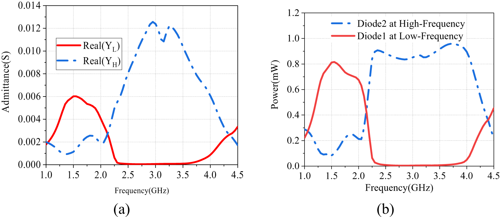
The admittance of the two branches of the rectifier at different frequencies is shown in Figure 5a. Figure 5b shows the distribution of RF power between the two diodes across different frequencies. Under a 0 dBm (1 mW) input, the majority of the RF power is directed to D 1 within the 1.1–2.2 GHz range. As the frequency increases, D 2 gradually dominates, receiving more than 80% of the power in the 2.2–4.1 GHz band, while the power loss in D 1 becomes negligible.
(a) The admittance of the two branches of the rectifier. (b) Simulation power of diodes 1 and 2 versus frequency.

Figure 5 Long description
Line graph with the y-axis labeled Admittance(S), ranging from 0.000 to 0.014 in increments of 0.002 and the x-axis labeled Frequency(GHz), ranging from 1.0 to 4.5 in increments of 0.5. A legend lists Real(YL) and Real(YH). Real(YL) rises from about 0.002 at 1.0 to about 0.006 near 1.5, then decreases to about 0.005 near 2.0, then drops to about 0.000 near 2.3 and stays near 0.000 until about 3.8, then rises to about 0.003 by 4.5. Real(YH) starts near 0.002 at 1.0, dips to about 0.001 near 1.3, rises to about 0.002 to 0.003 around 1.8 to 2.1, then increases to about 0.008 near 2.5, reaches about 0.012 to 0.013 around 3.0 to 3.4, then decreases to about 0.008 near 3.8 and to about 0.002 by 4.5. Line graph with the y-axis labeled Power(mW), ranging from 0.0 to 1.2 in increments of 0.2 and the x-axis labeled Frequency(GHz), ranging from 1.0 to 4.5 in increments of 0.5. A legend lists Diode2 at High-Frequency and Diode1 at Low-Frequency. Diode1 at Low-Frequency rises from about 0.2 at 1.0 to about 0.8 near 1.5, then decreases to about 0.7 near 2.0, then drops to about 0.0 near 2.3 and stays near 0.0 until about 3.8, then rises to about 0.45 by 4.5. Diode2 at High-Frequency is about 0.25 at 1.0, dips to about 0.1 near 1.4, rises to about 0.25 near 2.0, then increases to about 0.9 near 2.4, stays around about 0.85 to 0.95 from about 2.5 to 4.0, peaks near about 1.0 around 3.8 to 4.0, then decreases to about 0.25 by 4.5.
The input impedance responses of the diodes under 0 dBm excitation are presented in Figure 6a. The impedance trajectories – denoted as Zin 1, Zin2, and Zinp are approximately symmetric to the real axis across their corresponding bands: 1.1–2.2 GHz for D 1, 2.2–4.0 GHz for D 2, and 1.1–4.0 GHz for the total network. A conjugate impedance pattern in which all three impedance curves approximately satisfy the matching requirements.
(a) Impedance transformation over 1–4.2 GHz of ultra-wideband rectifier at 0 dBm. (b) Z in over 1–4.2 GHz of ultra-wideband rectifier.

Figure 6 Long description
Smith charts illustrating impedance transformation of an ultra-wideband rectifier. The charts use normalized resistance and reactance, typically referenced to 50 ohms. In image A, impedance trajectories Zin1, Zin2 and Zinp are shown. Zin1 and Zin2 represent different input ports or matching networks, with Zin1 covering 1.1 to 2.2 gigahertz and Zin2 from 2.2 to 4.0 gigahertz. Zinp spans 1.1 to 4.0 gigahertz. Key frequency markers are at 1.1, 2.2 and 4 gigahertz, with impedance near r equals 1, x equals 0 at 2.2 gigahertz, indicating a closer match. In image B, impedance at 0 dBm and minus 8 dBm is compared. The 0 dBm trajectory forms a tighter loop near the center, suggesting a better match, while the minus 8 dBm trajectory extends outward, indicating higher reactance. Frequency markers at 1.1 and 4.2 gigahertz show impedance movement with frequency. The charts highlight how impedance changes with power levels and frequency, aiding in matching network design.
The three important frequencies of the rectifier were set to f 0 = 2.2 GHz, f 1 = 1.1 GHz, and f 2 = 4 GHz. The input impedances Zin(f 1) and Zin(f 2) were obtained and calculated in Equation (14), and θ 0 was obtained. Then, substituting Zin(f 0) into Equation (5) yields Ze. Employing Equations (15) and (16) establishes B 0(f₁)/B 0(f₂) = f₂/f₁, and Zo was determined. At last, B 0 is calculated. Figure 6b illustrates the input impedance ZIN of the rectifier after applying the CMS. The results indicate excellent impedance matching across a wideband range of 1.3–4.1 GHz.
Implementation and measurements
Rectifier I
The layout and physical prototype of the broadband rectifier are shown in Figure 7 with an F4B-2 substrate (dielectric constant of 2.65 and loss tangent of 0.0012). The specific design parameters are detailed in Figure 7 as well, and the inductance of the susceptive element is 2.7 nH, and the diode is HSMS286.
Layout and photograph of the rectifier with parameter details.

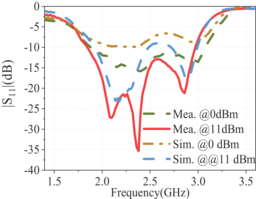
The simulated and measured S-parameters are presented in Figure 8, showing good agreement between simulation and measurement. For input power levels of 0 dBm and 11 dBm, the measured |S11| remains below −10 dB over the frequency range of 1.8–3.0 GHz, indicating effective wideband impedance matching.
S-parameter curves of the broadband rectifier.

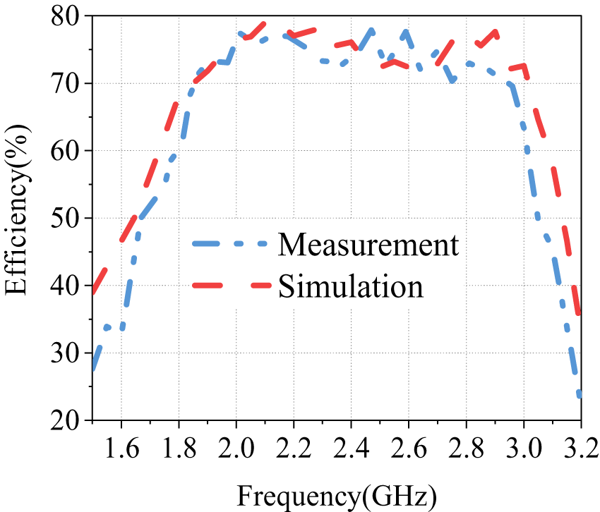
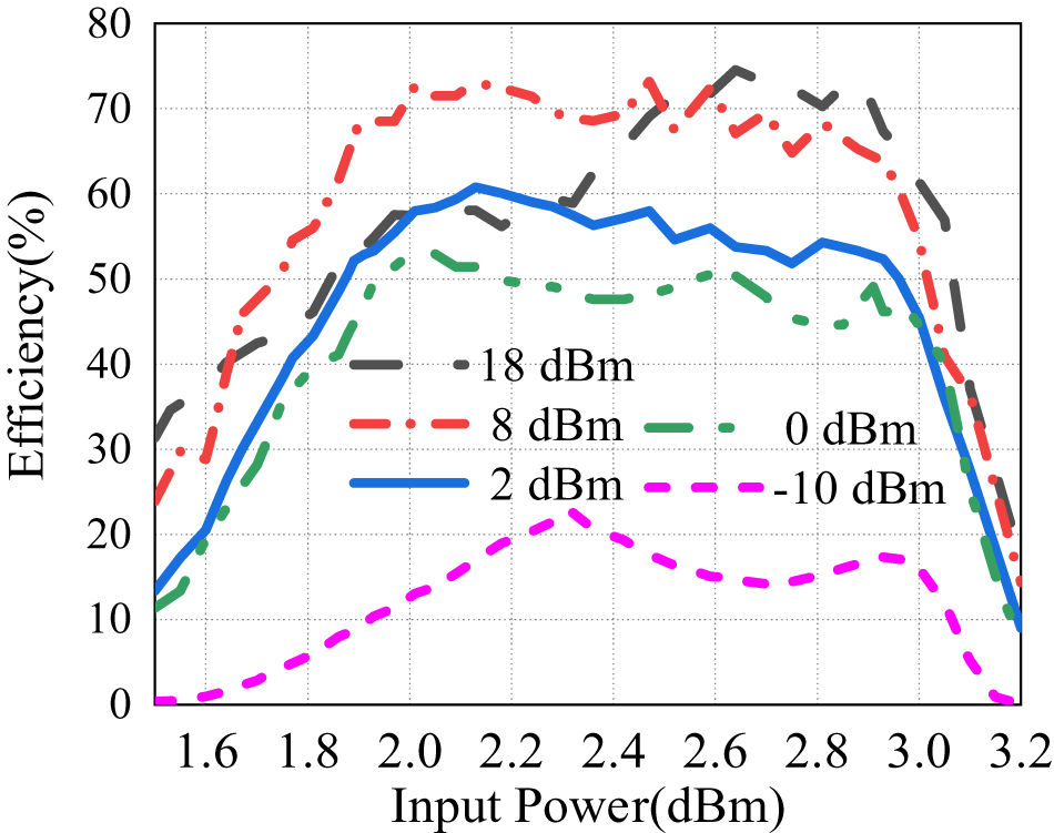
The rectifier power conversion efficiency was subsequently evaluated. Figure 9 compares the simulated and measured rectification efficiencies at an input power of 11 dBm with a 500 Ω DC load, demonstrating close agreement. The measured efficiency exceeds 70% across 1.8–3.0 GHz, corresponding to a fractional bandwidth of 50%. As shown in Figure 10, the efficiency remains above 50% from 1.88 to 2.98 GHz as the input power varies from 2 to 18 dBm.
Efficiency curves of broadband rectifier I at 11 dBm.

Efficiency curves of broadband rectifier I at different powers.

Figure 10 Long description
Efficiency(percent) Line graph with five curves and an in-plot legend. The x-axis is labeled Input Power(dBm), ranging from 1.6 to 3.2 with tick marks at 1.6, 1.8, 2.0, 2.2, 2.4, 2.6, 2.8, 3.0 and 3.2. The y-axis is labeled Efficiency(percent), ranging from 0 to 80 with tick marks at 0, 10, 20, 30, 40, 50, 60, 70 and 80. Legend entries: 18 dBm, 8 dBm, 0 dBm, 2 dBm, minus 10 dBm. 18 dBm curve: about 32 at 1.6; about 45 at 1.8; about 58 at 2.0; about 56 at 2.2; about 60 at 2.4; about 74 at 2.6; about 70 at 2.8; about 68 at 3.0; about 56 at 3.2. 8 dBm curve: about 30 at 1.6; about 55 at 1.8; about 72 at 2.0; about 72 at 2.2; about 69 at 2.4; about 70 at 2.6; about 68 at 2.8; about 62 at 3.0; about 15 at 3.2. 2 dBm curve: about 20 at 1.6; about 40 at 1.8; about 58 at 2.0; about 60 at 2.2; about 56 at 2.4; about 55 at 2.6; about 52 at 2.8; about 50 at 3.0; about 10 at 3.2. 0 dBm curve: about 18 at 1.6; about 38 at 1.8; about 52 at 2.0; about 50 at 2.2; about 47 at 2.4; about 50 at 2.6; about 45 at 2.8; about 45 at 3.0; about 12 at 3.2. Minus 10 dBm curve: about 0 at 1.6; about 5 at 1.8; about 12 at 2.0; about 18 at 2.2; about 20 at 2.4; about 15 at 2.6; about 15 at 2.8; about 17 at 3.0; about 0 at 3.2.
Ultra-wideband rectifier
The layout of the design and the photograph of the rectifier are shown in Figure 11a and 11b, respectively. It uses two SMS7630 diodes, and its total size is 18 × 24.8 mm.
(a) Layout of the proposed ultra-wideband rectifier. (b) Photograph of the fabricated ultra-wideband rectifier.

Figure 11 Long description
Printed circuit board layout with dimension arrows and the text Ground hole and Unit colon mm. A long horizontal dimension line along the bottom is labeled 18 mm and a long vertical dimension line along the right side is labeled 24.8mm. Near the lower left, a horizontal dimension is labeled 9.2 and the trace at the lower right corner turns upward with a vertical dimension labeled 10 and a width label 0.85 placed across the vertical trace. Near the center, two opposing triangular symbols meet at a narrow junction on the main horizontal trace, with one triangle above and one triangle below the junction. Above this junction, a vertical trace rises with a height label 8.3 and a width label 1.0 across the vertical trace and a small circular hole is drawn at the top end of this vertical trace. To the left of the central junction, two tall rectangular trace sections stand side by side, each with a vertical dimension label 7.8 and two horizontal spacing labels 2.0 and 1.1 are shown between and across these tall sections; a small curved coil symbol is drawn bridging the tops of the two tall sections. At the lower part of the left tall section, a narrow angled connection meets the main horizontal trace and a small dimension label 0.8 is placed near this angled connection. To the right of the central junction on the main horizontal trace, a small coil symbol is drawn on the trace and above that area a small rectangular component outline is shown with two circular holes inside it. Several circular holes appear at trace ends and corners, matching the Ground hole marker. Fabricated board with a central cross shaped metal trace and several soldered components mounted on it. A coaxial style connector is attached at the left edge of the board and connects into the metal trace and another connector is attached at the right edge and connects into the trace. Two small rectangular surface mounted components are visible near the central junction area of the trace and additional solder joints appear at bends and junctions. A long L shaped metal trace runs from the lower left area toward the bottom edge and then upward toward the center, ending near the central junction region.
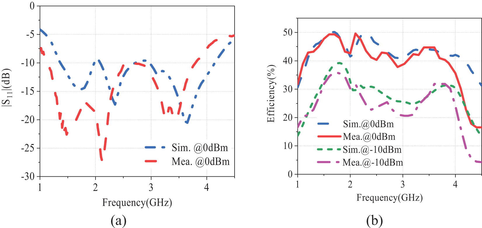
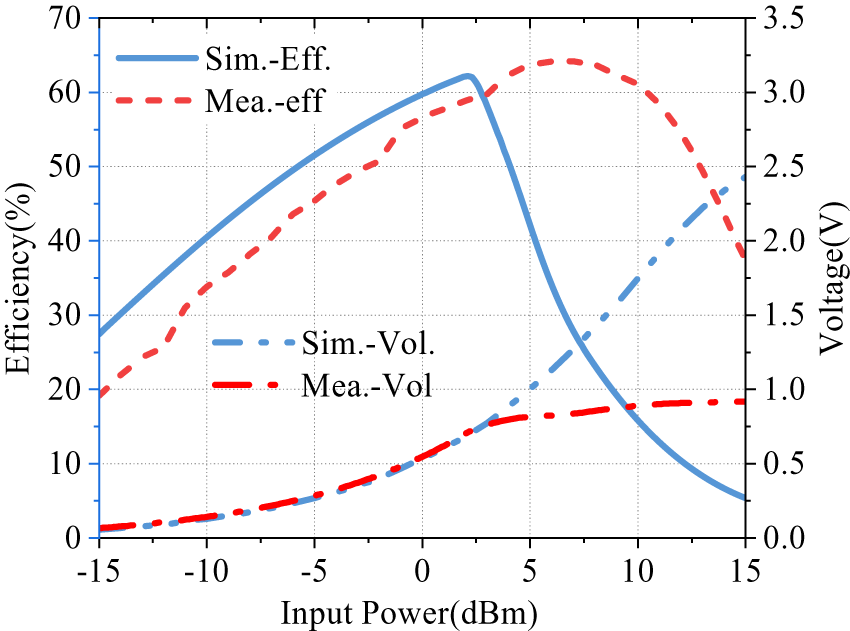
The measured reflection coefficient |S 11| at an input power of 11 dBm is presented in Figure 12a. At an input of 0 dBm, the ultra-wideband rectifier exhibits excellent impedance matching, with |S 11| remaining below −10 dB over the 1.1–3.9 GHz frequency range, thereby confirming its wideband matching performance. The RF-to-DC conversion efficiency versus frequency at input power levels of 0 dBm and −8 dBm is shown in Figure 12b, measured with a 200 Ω load. At 0 dBm, the rectifier achieves over 40% efficiency across the 1.1–3.9 GHz band, corresponding to a fractional bandwidth of 112%. Even at a reduced input power of −8 dBm, the efficiency remains above 20% over the extended frequency range of 1.05–4.05 GHz, highlighting the rectifier’s robust low-power performance. Figure 13 illustrates the variation in efficiency as a function of input power. The highest recorded efficiency is 64.2% at 1.7 GHz.
(a) The reflection coefficient |S11| of the ultra-wideband rectifier at 0 dBm. (b) RF-dc conversion efficiency versus frequency simulated and measured at 0 dBm and −8 dBm of the rectifier.

Figure 12 Long description
Line graph with the vertical axis label “|S11| (dB)” and tick labels 0, minus 5, minus 10, minus 15, minus 20, minus 25, minus 30. The horizontal axis label is “Frequency(GHz)” with tick labels 1, 2, 3, 4. A legend lists “Sim.@0dBm” and “Mea.@0dBm”. The “Sim.@0dBm” curve passes through approximately: (1, minus 4), (1.5, minus 15), (2, minus 10), (2.3, minus 17), (2.8, minus 10), (3.2, minus 14), (3.6, minus 21), (4.0, minus 13), (4.5, minus 6). The “Mea.@0dBm” curve passes through approximately: (1, minus 7), (1.4, minus 23), (1.9, minus 17), (2.1, minus 27), (2.4, minus 11), (2.8, minus 10), (3.2, minus 19), (3.4, minus 18), (3.6, minus 20), (4.0, minus 8), (4.5, minus 5). The “Sim.@0dBm” curve shows dips near 1.5, 2.3 and 3.6 on the frequency axis, with the lowest listed point at (3.6, minus 21). The “Mea.@0dBm” curve shows a deeper dip near 2.1 on the frequency axis, with the lowest listed point at (2.1, minus 27). Line graph with the vertical axis label “Efficiency(%)” and tick labels 0, 10, 20, 30, 40, 50. The horizontal axis label is “Frequency(GHz)” with tick labels 1, 2, 3, 4. A legend lists “Sim.@0dBm”, “Mea.@0dBm”, “Sim.@-10dBm” and “Mea.@-10dBm”. The “Sim.@0dBm” curve passes through approximately: (1.0, 30), (1.5, 47), (1.8, 50), (2.0, 42), (2.3, 49), (2.6, 43), (3.0, 40), (3.4, 44), (3.7, 44), (4.0, 41), (4.5, 32). The “Mea.@0dBm” curve passes through approximately: (1.0, 30), (1.5, 46), (1.8, 50), (2.0, 42), (2.2, 50), (2.5, 41), (2.9, 38), (3.3, 43), (3.7, 44), (4.0, 39), (4.3, 18), (4.5, 16). The “Sim.@-10dBm” curve passes through approximately: (1.0, 14), (1.5, 32), (1.8, 39), (2.0, 30), (2.4, 30), (2.8, 26), (3.2, 25), (3.6, 27), (3.9, 31), (4.2, 22), (4.5, 14). The “Mea.@-10dBm” curve passes through approximately: (1.0, 15), (1.5, 30), (1.8, 36), (2.0, 30), (2.4, 23), (2.8, 21), (3.2, 21), (3.6, 25), (3.9, 32), (4.1, 30), (4.3, 8), (4.5, 5). For 0 decibel milliwatt, the highest listed efficiency values are 50 at (1.8, 50) for “Sim.@0dBm” and 50 at (1.8, 50) and (2.2, 50) for “Mea.@0dBm”. For minus 10 decibel milliwatt, the highest listed efficiency values are 39 at (1.8, 39) for “Sim.@-10dBm” and 36 at (1.8, 36) for “Mea.@-10dBm”. The “Mea.@0dBm” and “Mea.@-10dBm” curves show lower listed values near 4.3 to 4.5 on the frequency axis, including (4.3, 18) and (4.5, 16) for “Mea.@0dBm” and (4.3, 8) and (4.5, 5) for “Mea.@-10dBm”. Both graphs use the same horizontal axis label “Frequency(GHz)”. The first graph plots “|S11| (dB)” for “Sim.@0dBm” and “Mea.@0dBm”. The second graph plots “Efficiency(%)” for “Sim.@0dBm”, “Mea.@0dBm”, “Sim.@-10dBm” and “Mea.@-10dBm”.
Conversion efficiency and output dc voltage at 1.7 GHz.

Figure 13 Long description
Input Power(dBm) on the horizontal axis with labeled ticks at minus 15, minus 10, minus 5, 0, 5, 10, 15. Left vertical axis label: Efficiency(percent). Labeled ticks from 0 to 70. Right vertical axis label: Voltage(V). Labeled ticks from 0.0 to 3.5. Legend text: Sim.-Eff., Mea.-eff, Sim.-Vol., Mea.-Vol. Sim.-Eff. coordinate pairs: (minus 15, 28), (minus 10, 40), (minus 5, 51), (0, 60), (2, 62), (5, 40), (10, 15), (15, 5) Mea.-eff coordinate pairs: (minus 15, 20), (minus 10, 33), (minus 5, 45), (0, 56), (3, 60), (5, 63), (7, 64), (10, 61), (12, 55), (15, 38) Sim.-Vol. coordinate pairs: (minus 15, 0.05), (minus 10, 0.15), (minus 5, 0.30), (0, 0.55), (5, 1.00), (10, 1.75), (15, 2.45) Mea.-Vol. coordinate pairs: (minus 15, 0.05), (minus 10, 0.15), (minus 5, 0.30), (0, 0.55), (5, 0.80), (10, 0.90), (15, 0.95).
Table 1 compares the performance with previous publications for ultra-wide bands. The fractional bandwidths of the proposed rectifiers are in the leading position, while their physical dimensions are much less than those of rectifiers of similar types. Rectifiers designed with CMS ensure high rectification efficiency and wide operating bandwidth at low and medium power levels while effectively reducing the physical size of the rectifier circuit.
Comparison between ultra-wide rectifiers

Table 1 Long description
Ultrawide rectifier designs are compared by diode type, required input power, target efficiency, operating band range, fractional bandwidth, physical size, and diode count. This work uses an SMS7630 diode pair and targets 40 percent efficiency at 0 dBm over 1.1 to 3.9 GHz, the widest band listed, with 112 percent fractional bandwidth and an 18 by 25 mm footprint. The next widest bandwidth is 107.7 percent for an HSMS2850 design covering 0.32 to 0.92 GHz, requiring 6 dBm and using one diode, but it is much larger at 38 by 100 mm. Other wideband entries include 104 percent from 1.2 to 3.2 GHz using four SMS7630 diodes with size not available, and 100 percent from 0.8 to 2.4 GHz at 0 dBm using two SMS7630 diodes in a 32 by 14 mm layout. Narrower bands include 40.7 percent from 1.82 to 2.75 GHz that requires 8 to 25 dBm and targets 50 percent efficiency, and 75.36 percent from 0.43 to 0.95 GHz with a very large 190 by 30 mm size. Several entries mark the 40 percent efficiency requirement with an asterisk, so efficiency conditions may differ and should be checked in the original sources. Sizes are reported as length by width in millimeters, and one entry lists size as not available.
Conclusion
This paper proposes a novel design for wideband rectifiers. A band-stop structure is applied to tune the diode impedance and enhance the conversion efficiency. A coupled matching structure successfully matches it to the system impedance within a wide bandwidth. We explored the mechanism and presented the design methods.
Two wideband rectifiers were designed, fabricated, and measured to verify the proposed design method. The operating bandwidths of the two rectifiers are from 1.83 to 2.95 GHz and from 1.1 to 3.9 GHz, respectively. They have very compact physical dimensions as well. The design methodology helps facilitate the design of wide-band compact rectifiers and makes them easier to integrate into antennas. They have a bright future in the applications of wireless power transmission and EH systems.
Acknowledgements
This work was supported in part by the Natural Science Foundation of China (NSFC) under Grants U22A2015 and 62401382 and JCKY.
Author contributions
D.Z. and C.L. derived the theory; H.H. and Z.H. performed the simulations. All authors contributed equally to analyzing data and reaching conclusions and in writing the paper.
Competing interest
The authors declare none.

Dejin Zhu received the M.S. degree in radio physics from Sichuan University, Chengdu, China, in 2006, where he is currently pursuing the Eng.D. degree in electronic information. His main research interests are the design and optimization of sensors and wireless power transmission.

Haoming He received the S. and M.S. degrees from Sichuan University, Chengdu, China, in 2020 and 2023, respectively, where he is currently pursuing the Ph.D. degree in Electronic Science and Technology. His current research interests include wireless power transmission and energy harvesting.

Zhongqi He received the M.S. degree and the Ph.D. degree in radio physics from Sichuan University, Chengdu, China, in 2018 and 2023, respectively. From 2021 to 2022, he was a visiting scholar at the University of Bologna, Italy. In 2023, he joined the College of Electronics and Information Engineering, Sichuan University, where he has been an associate research fellow since May 2025.
He has authored more than 20 papers published in peer-reviewed journals and international conferences. His current research interests include wireless power transmission and energy harvesting.

Chongwei Liao received the B.S. degree in electronic information science and technology from Chengdu University of Information Technology, Sichuan, China, in 2017, and the M.S. degree in electromagnetic fields and microwave technology and the Eng.D. degree in electronic information from Sichuan University, Sichuan, China, in 2021 and 2025, respectively.
His current research interests include industrial applications of microwave energy, microwave intelligent control, and microwave measurement.

Changjun Liu received the M.S. and Ph.D. degrees from Sichuan University, China, in 1997 and 2000, respectively. From 2000 to 2001, he was a post-doctoral researcher at Seoul National University, Korea. From 2006 to 2007, he was a visiting scholar at Ulm University, Germany. Since 1997, he has been with the Department of Radio-Electronics, Sichuan University, where he has been a professor since 2004. He has authored two books and more than 200 articles. His current research interests include microwave wireless power transmission and microwave power industrial applications. Dr. Liu was a recipient of the Outstanding Reviewer of the IEEE Transactions on Microwave Theory and Techniques from 2006 to 2010. He is a member of IEEE MTT-S TC 25 and serves as a topic editor of the IEEE Journal of Microwave. He also serves as the editor-in-chief of Microwave.