1 Introduction
A general magnetic field due to an arbitrary steady distribution of electric charges (Stratton Reference Stratton1941) leads to a vector Poisson equation, whose solution is a multipolar expansion (Kellogg Reference Kellogg1953; MacMillan Reference MacMillan1958). The multipolar expansion extends to electromagnetic waves due to unsteady electric charges and currents as a solution of the forced wave equation (Landau & Lifshitz Reference Landau and Lifshitz1987). Since the multipolar expansion is considered only for the background magnetic field, the steady case (Campos Reference Campos2014) is reconsidered briefly (see appendix A), showing that the higher-order terms are important in the near field, whereas the far field is dominated by the lowest-order term, that decays more slowly, like a dipole (Campos Reference Campos2011). For this reason, the simplest far-field model of the magnetic field of the Earth, Sun and other celestial bodies is a magnetic dipole. The monopole that exists for an irrotational field cannot exist for solenoidal fields, because it does not meet the conservation of magnetic flux across a closed surface unless a split monopole is used. The dipolar magnetic far field of most celestial bodies permeates a plasma, like the ionosphere of the Earth or the atmosphere of the Sun and other stars. A plasma can support Alfvén waves (Alfvén Reference Alfvén1942, Reference Alfvén1947, Reference Alfvén1950; Alfvén & Fälthammar Reference Alfvén and Fälthammar1963; Campos Reference Campos1977, Reference Campos1987, Reference Campos1997, Reference Campos1998) that are transverse hydromagnetic motions propagating along magnetic field lines. This motivates the study of Alfvén waves propagating along the field lines of a magnetic dipole, using a new orthogonal curvilinear coordinate system: dipolar coordinates. Conformal coordinates are specified by the real and imaginary parts of a complex analytic function; it follows immediately that they are a plane orthogonal coordinate system, with equal scale factors along the two (generally curvilinear) coordinate axes. It can be readily shown that the common scale factor is the modulus of the inverse of the function’s derivative. Among the conformal coordinates, only four allow separation of variables in the two-dimensional Laplace operator, namely (Morse & Feshbach Reference Morse and Feshbach1953): Cartesian, polar, parabolic and confocal. Besides these four best known of plane orthogonal coordinate systems, there are many others, exempli gratia (e.g.) every analytic function specifies one. An example is spiral coordinates (Campos & Gil Reference Campos and Gil1995), and in the present paper another example is considered, videlicet (viz.) multipolar coordinates (see § 2.1).
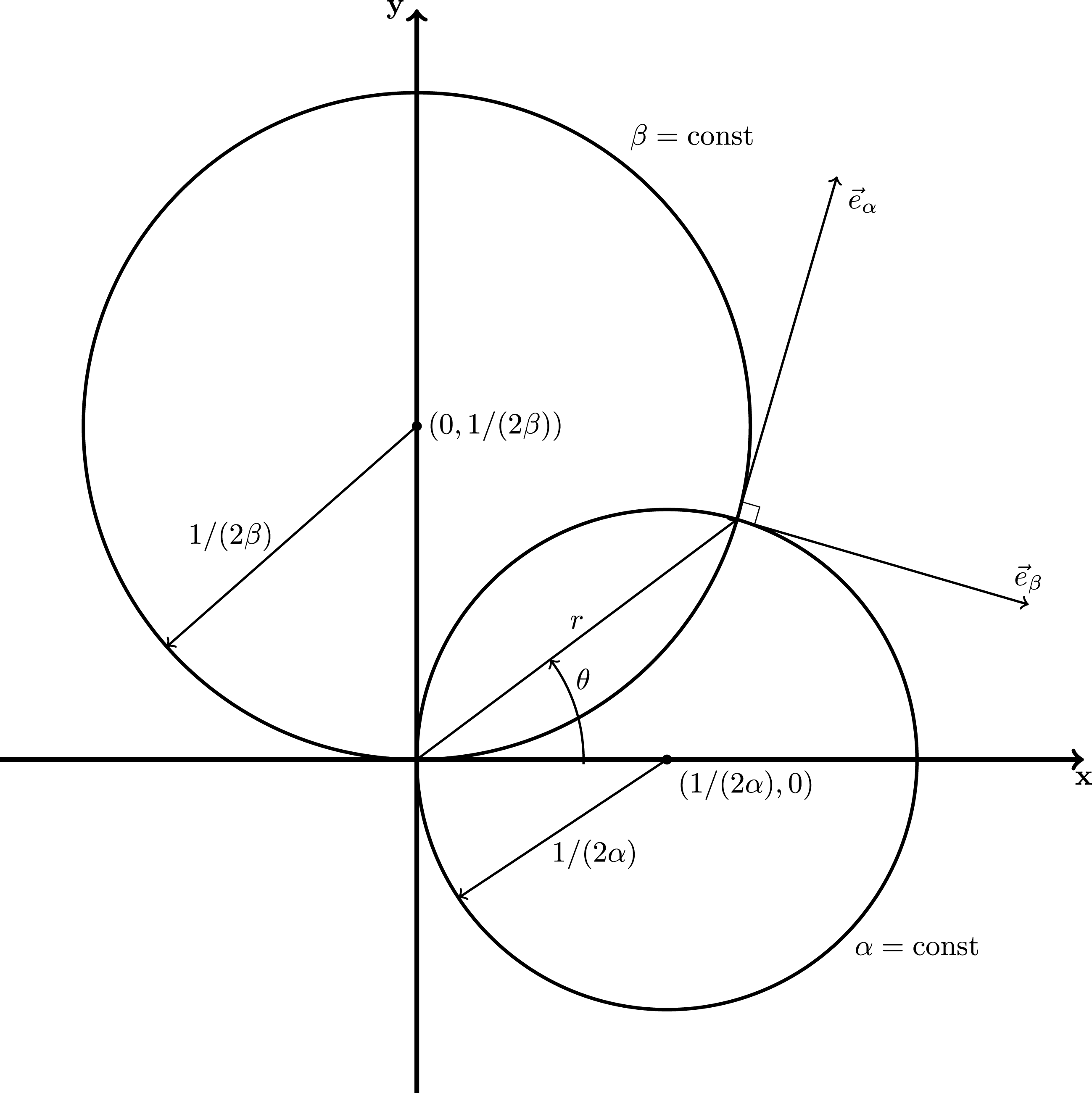
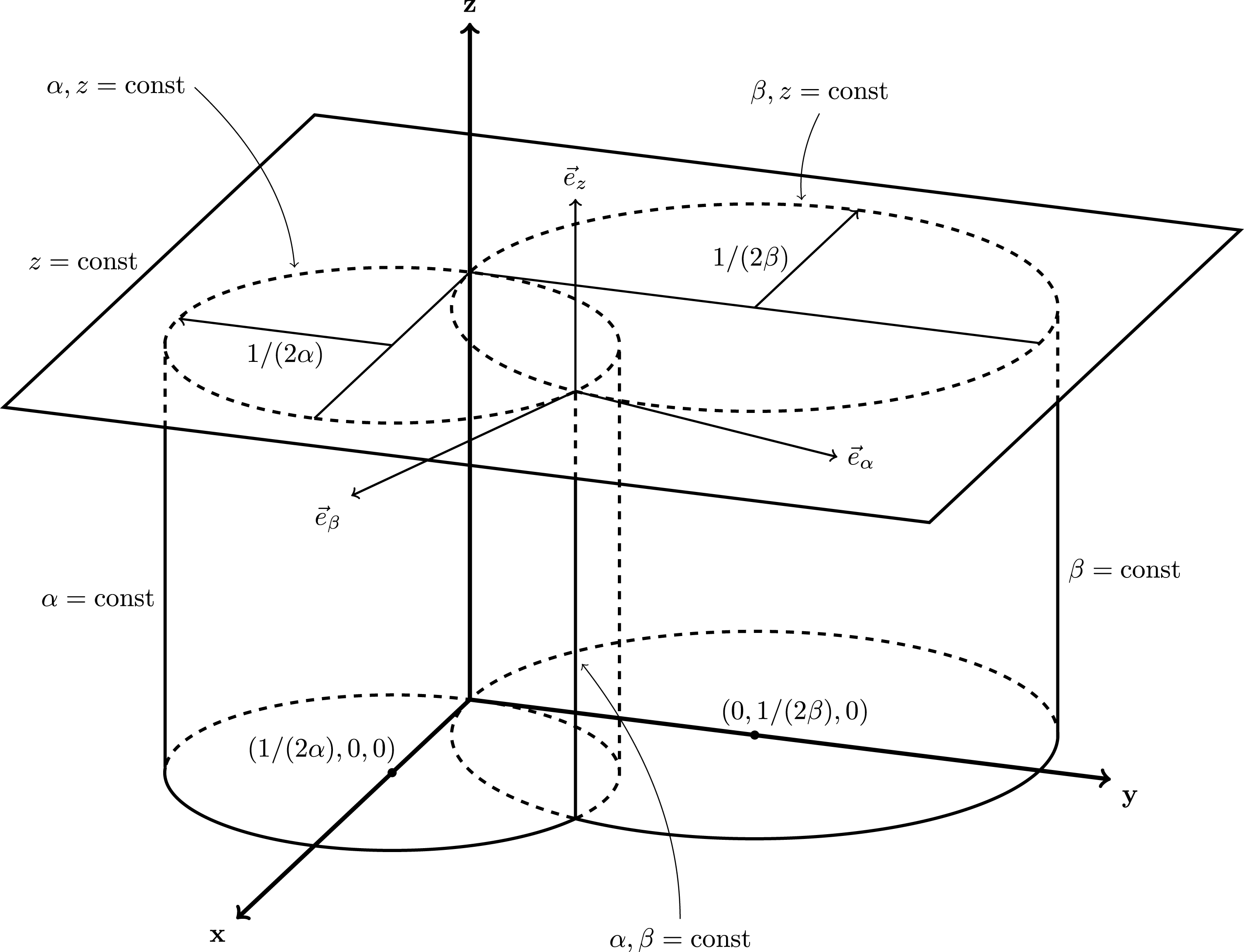
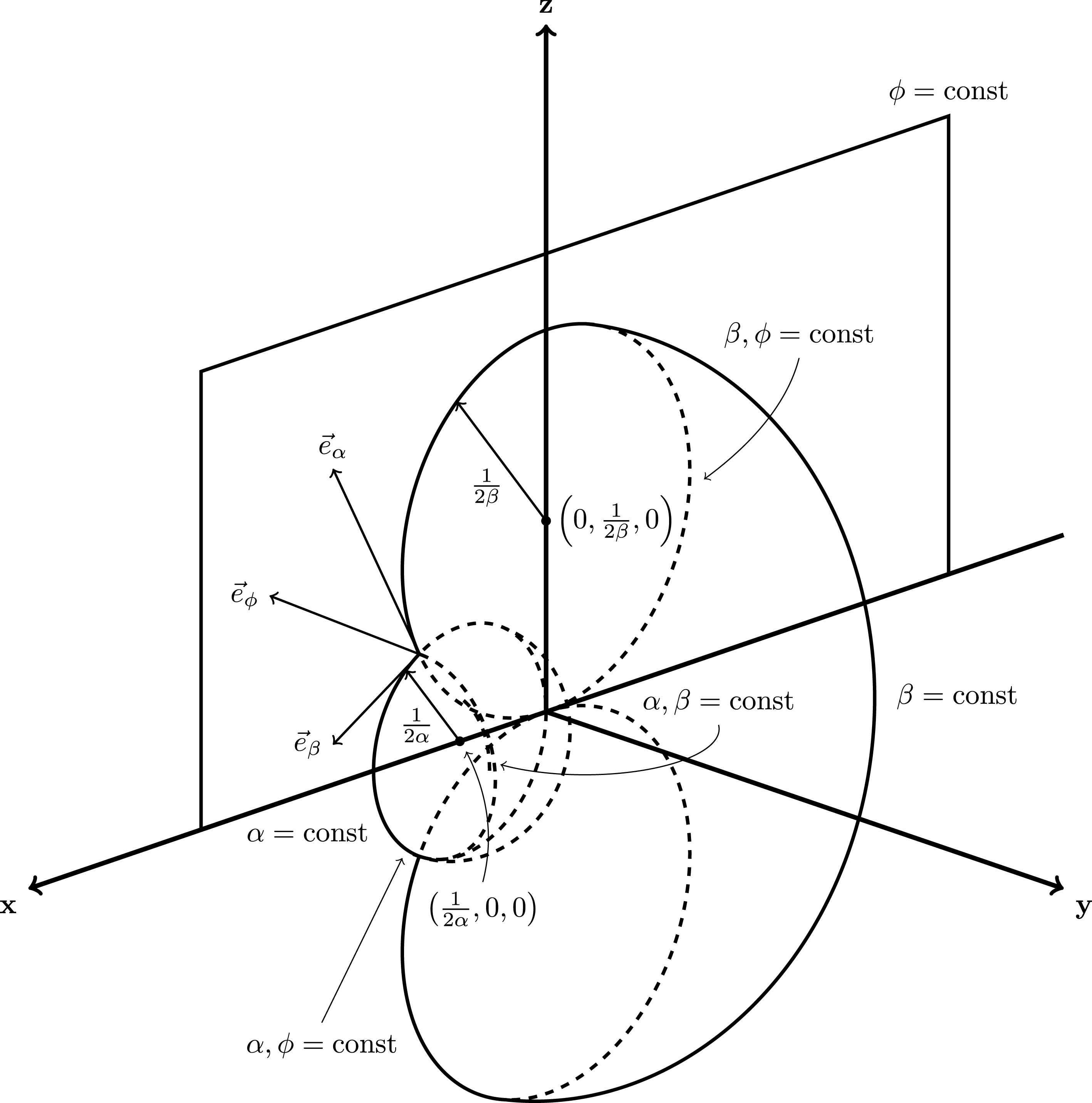
A particular case is dipolar coordinates (see § 2.2) for which the two sets of coordinate curves (figure 1) are circles with the centre on one coordinate axis and tangent to the other. These coordinate systems are particularly convenient for problems for which quantities vary only along one of the coordinate curves, e.g. Alfvén waves propagating along a spiral (Campos & Gil Reference Campos and Gil1995), as relevant to the magnetic field in the solar wind, or along a circle (see § 3.1), as relevant to the Earth’s dipolar magnetic field (see § 2.3), in the present paper. The exact analytical solution of the Alfvén wave equation in conformal coordinates depends on the scale factor, and is distinct for different coordinate systems, for example the propagation along a logarithmic spiral is specified by Bessel functions, whereas in the present case of propagation along a circle an extended form of the Gaussian hypergeometric function is needed (see § 3.2). The original Gaussian hypergeometric differential equation has three regular singularities (Forsyth Reference Forsyth1956), however, in the present case, an extended form appears for which one of the singularities is irregular. The extended Gaussian hypergeometric differential equation has series solutions, whose recurrence formulas for the coefficients are less simple than the original; using these solutions, the velocity and magnetic field perturbations spectra of the Alfvén waves (see § 4.1) are computed and plotted (figures 3 to 6), for several values of the dimensionless frequency (see § 5), which is the only parameter in the problem.
The dipolar coordinates in the plane have, for coordinate curves, circles with centres on one axis tangent to the other axis forming two families of orthogonal curves with the same conformal scale factor.

In terms of mathematical complexity, Alfvén waves propagating along a circle are one echelon above the cases solvable using (I) elementary functions, (II) Bessel functions and (III) Gaussian hypergeometric functions. The first class (I) of problems, solvable in terms of elementary functions, concerns non-dissipative (Alfvén Reference Alfvén1950; Baños Jr Reference Baños1955; Lighthill Reference Lighthill1960; Cabannes Reference Cabannes1970) and dissipative (Alfvén Reference Alfvén1947; Cowling Reference Cowling1957; Alfvén & Fälthammar Reference Alfvén and Fälthammar1963; Campos Reference Campos1977, Reference Campos1999; Moffatt Reference Moffatt1978) Alfvén waves in homogeneous media, for which the wave speed and diffusivities are constant. The second class (II) of problems, solvable in terms of Bessel functions, includes Alfvén waves in an isothermal atmosphere, under a uniform background magnetic field (Ferraro & Plumpton Reference Ferraro and Plumpton1958, Reference Ferraro and Plumpton1966; Hollweg Reference Hollweg1972, Reference Hollweg1978; Leroy Reference Leroy1980; Campos Reference Campos1983a ; Schwartz, Cally & Bel Reference Schwartz, Cally and Bel1984; Campos Reference Campos1987, Reference Campos1998), as well as extensions to include displacement (Leroy Reference Leroy1983) and Hall (Campos Reference Campos1992) currents; other cases include Alfvén waves in a linear temperature gradient (Zhugzhda Reference Zhugzhda1971), and spherical Alfvén waves (Campos Reference Campos1994). The third class (III) of problems, solvable using Gaussian hypergeometric functions, concerns Alfvén waves with a critical layer, viz. due to the Hall effect (Campos & Isaeva Reference Campos and Isaeva1992), and viscous and resistive dissipation (Campos Reference Campos1983c ,Reference Campos b , Reference Campos1988b , Reference Campos1989, Reference Campos1993a ,Reference Campos b ). Other methods have been used to study Alfvén waves in a non-uniform background magnetic field (Oliver et al. Reference Oliver, Ballester, Hood and Priest1993; Lou Reference Lou1994), in moving media (Whang Reference Whang1973; McKenzie, IP & Axford Reference McKenzie, IP and Axford1979; Velli Reference Velli1993; McKenzie Reference McKenzie1994) and in the presence of viscous and resistive dissipation (Priest & Heyvaerts Reference Priest and Heyvaerts1983; Nocera, Leroy & Priest Reference Nocera, Leroy and Priest1984; Nocera, Priest & Hollweg Reference Nocera, Priest and Hollweg1986).
The theoretical developments of Alfvén waves can be fundamental to understanding some features taking place in the Earth’s magnetosphere. Plasma turbulence exists in space and astrophysical plasmas under some conditions (Bruno & Carbone Reference Bruno and Carbone2005), and therefore the study of magnetic field fluctuations is important because they influence the dynamics of the Earth’s magnetosphere, the energy and mass inflows from the solar wind to the magnetosphere and, at the atomic scale, the heating and acceleration of particles. The solar wind influences the plasma processes within the magnetosheath and this research topic is significant to understanding the plasma turbulence close to the Earth. A comparison between experimental results and simulations is undertaken by several researchers. For instance, in the work by Dwivedi et al. (Reference Dwivedi, Kumar, Kovacs, Yordanova, Echim, Sharma, Khodachenko and Sasunov2019), the measurement of magnetic field turbulence spectra in the magnetosheath region of the Earth obtained by the Cluster-1 magnetometer (Balogh et al. Reference Balogh, Carr, Acuña, Dunlop, Beek, Brown, Fornacon, Georgescu, Glassmeier and Harris2001) and the Cluster Ion Spectroscopy experiment (Rème Reference Rème2001) are compared with the numerical results obtained by the two-fluid model and the dynamical equations of kinetic Alfvén waves to research the turbulent dynamics of the magnetosheath plasma using spectral analysis of magnetic field fluctuations. Otherwise, the nonlinear kinetic Alfvén waves can describe the nature of small-scale turbulence. The processes of particles acceleration at the Earth’s bow shock and Alfvén wave generation by accelerated particles are also investigated in several research articles (Lee Reference Lee1982; Scholer, Kucharek & Trattner Reference Scholer, Kucharek and Trattner1999), by comparing calculated spectra of accelerated ions with the experimentally observed spectra of accelerated ions (Ellison, Möbius & Paschmann Reference Ellison, Möbius and Paschmann1990). These processes are accompanied by a significant increase in the level of turbulence induced by Alfvén waves and therefore a consistent description must include the generation of these waves by accelerated ions. For instance, the paper by Berezhko & Taneev (Reference Berezhko and Taneev2007) shows that using a refined growth rate of the Alfvén waves excited by accelerated particles based on results from Gordon et al. (Reference Gordon, Lee, Möbius and Trattner1999), yields that, while the equilibrium state is approached, the amplitude of Alfvén waves increases monotonically and the comparison between the calculated accelerated ions and Alfvénic turbulence spectra with the measurements shows that the theory agrees well with the main features observed in experiments.
There is conjointly an enormous quantity of research devoted to studying the problem of determining a relationship between the field of Alfvén waves and electromagnetic oscillations on the Earth’s ground. A theoretical treatment of the penetration of the Alfvén wave field from the magnetosphere to the ground through the ionosphere and atmosphere is formed in several articles (Greifinger Reference Greifinger1972; Belyaev et al. Reference Belyaev, Polyakov, Rapoport and Trakhtengerts1990; Leonovich & Mazur Reference Leonovich and Mazur1991). The ionospheric effects in the Alfvén wave penetration method are also explained briefly in these papers, since they act to drive currents within the ionospheric layer which are associated with magnetosound waves inducing the pulsations on the ground. These effects act differently depending upon the frequency of the waves. Particularly, in the work by Leonovich & Mazur (Reference Leonovich and Mazur1996), the boundary conditions on the ionosphere for standing Alfvén waves and the analytical expressions to describe the field of electromagnetic oscillations induced on the terrestrial surface by the same waves in the magnetosphere have been obtained. It was also concluded that the process of penetration to the ground of the poloidal part of the electromagnetic field originated from the magnetospheric Alfvén oscillations is induced mainly by the Pedersen conductivity of the ionosphere. A numerical model, used by Fedorov et al. (Reference Fedorov, Mazur, Pilipenko and Engebretson2016), of the magnetospheric Alfvén wave interaction with the ionosphere and penetration to the ground based on the solution of multi-fluid magnetohydrodynamic full wave equations in a realistic ionosphere was developed. This model predicts that the upper part of the Pc1 spectrum (approximately 0.2 to 5 Hz) is severely absorbed upon wave transmission through the daytime ionosphere to the ground. At night time, the transmission coefficient of Alfvén waves has an oscillatory dependence on frequency. Moreover, modelling the ground signatures of waves externally generated in the outer magnetosphere, such as Pc1 oscillations, is complicated because the electromagnetic skin depth (Jackson Reference Jackson1975) is comparable to the ionospheric thickness and, consequently, resolving the vertical structure of the ionosphere is necessary. Furthermore, in the ionosphere, the Hall conductivity and shear Alfvén waves are coupled to compressional mode waves that can propagate across field lines. In the model developed by Lysak (Reference Lysak1997), the interactions of Alfvén waves can be described in the 1 Hz frequency band with the ionosphere. These interactions can determine the ground observations of Pc1 oscillations not only on the field lines on which they are generated but also as they propagate horizontally through the ionospheric waveguide. A strong point in that model is the ability to determine the ground magnetic field produced by a model run and to compare these fields with the fields produced on the ground. Some well-known results, such as the ‘Hughes rotation’ of the magnetic field, the production of 1 Hz waves by the inhomogeneity of the ionosphere and the ducting of compressional waves through an ionospheric waveguide, have been reproduced by the model.
These works prove therefore that developing mathematical models that can describe the propagation of the Alfvén waves can be useful to prove some experimental results provided by observations on the ground and this paper, therefore, intends to construct a model that describes the Alfvén waves propagating along a dipolar magnetic field.
2 Conformal coordinates and atmospheric equilibrium
Among the conformal coordinates (see § 2.1), the dipolar coordinates are chosen (see § 2.2). The atmospheric equilibrium is also adopted (see § 2.3) as a preliminary to the consideration of Alfvén wave propagation.
2.1 Conformal coordinates and equal scale factors
Conformal coordinates (
 $\unicode[STIX]{x1D6FC}$
,
 $\unicode[STIX]{x1D6FD}$
) are specified by the real and imaginary parts of a complex function
 $w$
,
 $$\begin{eqnarray}\unicode[STIX]{x1D6FC}-\text{i}\unicode[STIX]{x1D6FD}\equiv w=f(z),\end{eqnarray}$$
which specifies its relation with Cartesian (
 $x$
,
 $y$
) or polar (
 $r$
,
 $\unicode[STIX]{x1D703}$
) coordinates
 $$\begin{eqnarray}z=x+\text{i}y=r\text{e}^{\text{i}\unicode[STIX]{x1D703}}.\end{eqnarray}$$
If the function is analytic,
 $$\begin{eqnarray}\text{d}w=\left(\frac{\text{d}f}{\text{d}z}\right)\text{d}z,\end{eqnarray}$$
then the arclength
 $$\begin{eqnarray}(\text{d}l)^{2}=|\text{d}z|^{2}=\left|\frac{\text{d}f}{\text{d}z}\right|^{-2}|\text{d}w|^{2}\end{eqnarray}$$
is given by
 $$\begin{eqnarray}(\text{d}l)^{2}=s^{2}\left[(\text{d}\unicode[STIX]{x1D6FC})^{2}+(\text{d}\unicode[STIX]{x1D6FD})^{2}\right],\end{eqnarray}$$
which shows that the conformal coordinate system is orthogonal (no
 $\text{d}\unicode[STIX]{x1D6FC}\text{d}\unicode[STIX]{x1D6FD}$
term) and the scale factor
 $s$
is the same along both coordinate axes,
 $$\begin{eqnarray}s\equiv \left|\frac{\text{d}f}{\text{d}z}\right|^{-1}=\left|\frac{\text{d}w}{\text{d}z}\right|^{-1},\end{eqnarray}$$
and equal to the modulus of the inverse of the function’s derivative.
As an example, reconsider spiral coordinates (Campos & Gil Reference Campos and Gil1995) which can be specified by the complex function
 $$\begin{eqnarray}w=(1+\text{i}k)\log z\end{eqnarray}$$
where
 $k$
is a constant. It follows from
 $$\begin{eqnarray}\unicode[STIX]{x1D6FC}=\log r-k\unicode[STIX]{x1D703},\quad -\unicode[STIX]{x1D6FD}=k\log r+\unicode[STIX]{x1D703},\end{eqnarray}$$
that coordinate curves of
 $\unicode[STIX]{x1D6FC}$
and
 $\unicode[STIX]{x1D6FD}$
are logarithmic spirals,
 $$\begin{eqnarray}\displaystyle & \displaystyle \frac{1}{r}\left(\frac{\text{d}r}{\text{d}\unicode[STIX]{x1D703}}\right)_{\unicode[STIX]{x1D6FC}}=k\equiv \cot \unicode[STIX]{x1D719}, & \displaystyle\end{eqnarray}$$
 $$\begin{eqnarray}\displaystyle & \displaystyle \frac{1}{r}\left(\frac{\text{d}r}{\text{d}\unicode[STIX]{x1D703}}\right)_{\unicode[STIX]{x1D6FD}}=-\frac{1}{k}=-\tan \unicode[STIX]{x1D719}=\cot \left(\unicode[STIX]{x1D719}+\frac{\unicode[STIX]{x03C0}}{2}\right), & \displaystyle\end{eqnarray}$$
 $\unicode[STIX]{x1D719}\equiv \arctan (1/k)$
and
 $\unicode[STIX]{x03C0}/2+\unicode[STIX]{x1D719}$
, with every radial line. The scale factor is given by (2.6) and (2.7), viz.
 $$\begin{eqnarray}s=\left|\frac{z}{1+\text{i}k}\right|=\frac{r}{\sqrt{1+k^{2}}},\end{eqnarray}$$
or using the inverse coordinate transformation
 $$\begin{eqnarray}r=\exp \left[\frac{\unicode[STIX]{x1D6FC}-k\unicode[STIX]{x1D6FD}}{1+k^{2}}\right],\quad \unicode[STIX]{x1D703}=-\frac{\unicode[STIX]{x1D6FD}+k\unicode[STIX]{x1D6FC}}{1+k^{2}},\end{eqnarray}$$
by
 $$\begin{eqnarray}s=\left|1+k^{2}\right|^{-1/2}\exp \left[\frac{\unicode[STIX]{x1D6FC}-k\unicode[STIX]{x1D6FD}}{1+k^{2}}\right].\end{eqnarray}$$
This result could have been obtained by substituting (2.11) in the arclength in polar coordinates,
 $$\begin{eqnarray}(\text{d}l)^{2}=(\text{d}r)^{2}+r^{2}(\text{d}\unicode[STIX]{x1D703})^{2},\end{eqnarray}$$
and then showing it takes the form (2.5) with
 $s$
given by (2.12).
As another example, consider multipolar coordinates, which are specified by
 $$\begin{eqnarray}w=z^{-n},\end{eqnarray}$$
with
 $n$
an integer. They relate (2.1) and (2.2) to polar coordinates by
 $$\begin{eqnarray}\unicode[STIX]{x1D6FC}=r^{-n}\cos (n\unicode[STIX]{x1D703}),\quad \unicode[STIX]{x1D6FD}=r^{-n}\sin (n\unicode[STIX]{x1D703}),\end{eqnarray}$$
whose inverse is
 $$\begin{eqnarray}\displaystyle & \displaystyle r=\left(\unicode[STIX]{x1D6FC}^{2}+\unicode[STIX]{x1D6FD}^{2}\right)^{-1/(2n)}, & \displaystyle\end{eqnarray}$$
 $$\begin{eqnarray}\displaystyle & \displaystyle \unicode[STIX]{x1D703}=\frac{1}{n}\arctan \left(\frac{\unicode[STIX]{x1D6FD}}{\unicode[STIX]{x1D6FC}}\right). & \displaystyle\end{eqnarray}$$
 $$\begin{eqnarray}s=\frac{1}{\left|-nz^{-n-1}\right|}=\frac{1}{n}r^{n+1}\end{eqnarray}$$
or, using (2.16a ),
 $$\begin{eqnarray}s=\frac{1}{n}\left(\unicode[STIX]{x1D6FC}^{2}+\unicode[STIX]{x1D6FD}^{2}\right)^{-1/2-1/(2n)}.\end{eqnarray}$$
This result could also be obtained by substituting both equations of (2.16) in (2.13), and writing it in the form (2.5) to show that the scale factors are given by (2.18).
2.2 Plane dipolar coordinates
Further consideration is given to the particular case
 $n=1$
of multipolar coordinates,
 $$\begin{eqnarray}w=\frac{1}{z}.\end{eqnarray}$$
Using (2.1) and (2.2), the transformation from polar (
 $r$
,
 $\unicode[STIX]{x1D703}$
) to dipolar (
 $\unicode[STIX]{x1D6FC}$
,
 $\unicode[STIX]{x1D6FD}$
) coordinates is
 $$\begin{eqnarray}\displaystyle & \displaystyle \unicode[STIX]{x1D6FC}=\frac{1}{r}\cos \unicode[STIX]{x1D703}, & \displaystyle\end{eqnarray}$$
 $$\begin{eqnarray}\displaystyle & \displaystyle \unicode[STIX]{x1D6FD}=\frac{1}{r}\sin \unicode[STIX]{x1D703}, & \displaystyle\end{eqnarray}$$
 $$\begin{eqnarray}\displaystyle & \displaystyle r=\frac{1}{\left|\unicode[STIX]{x1D6FC}^{2}+\unicode[STIX]{x1D6FD}^{2}\right|^{1/2}}, & \displaystyle\end{eqnarray}$$
 $$\begin{eqnarray}\displaystyle & \displaystyle \unicode[STIX]{x1D703}=\arctan \left(\frac{\unicode[STIX]{x1D6FD}}{\unicode[STIX]{x1D6FC}}\right). & \displaystyle\end{eqnarray}$$
The scale factor is
 $$\begin{eqnarray}s=\left|\frac{\text{d}(1/z)}{\text{d}z}\right|^{-1}=\left|z^{2}\right|=r^{2}\end{eqnarray}$$
in polar and
 $$\begin{eqnarray}s=\frac{1}{\unicode[STIX]{x1D6FC}^{2}+\unicode[STIX]{x1D6FD}^{2}}\end{eqnarray}$$
in dipolar coordinates, leading to
 $$\begin{eqnarray}(\text{d}l)^{2}=\frac{(\text{d}\unicode[STIX]{x1D6FC})^{2}+(\text{d}\unicode[STIX]{x1D6FD})^{2}}{\left(\unicode[STIX]{x1D6FC}^{2}+\unicode[STIX]{x1D6FD}^{2}\right)^{2}}\end{eqnarray}$$
as the dipolar arc element, according to (2.5).
The
 $\unicode[STIX]{x1D6FC}$
coordinate curve
 $$\begin{eqnarray}\unicode[STIX]{x1D6FC}=r^{-1}\cos \unicode[STIX]{x1D703}=\text{const.}\end{eqnarray}$$
is a circle (figure 1) with centre on the
 $OX$
axis at
 $(1/(2\unicode[STIX]{x1D6FC}),0)$
and radius
 $r=1/(2\unicode[STIX]{x1D6FC})$
such that it is tangent to the
 $OY$
axis at the origin, id est (i.e.) the diameter is given by
 $$\begin{eqnarray}R=1/\unicode[STIX]{x1D6FC}.\end{eqnarray}$$
The coordinate curve
 $\unicode[STIX]{x1D6FD}=\text{const.}$
is an orthogonal circle, with centre on the
 $OY$
axis at
 $(0,1/(2\unicode[STIX]{x1D6FD}))$
and radius
 $1/(2\unicode[STIX]{x1D6FD})$
such that it is tangent to the
 $OX$
axis at the origin.
Considering the wave propagation along the
 $\unicode[STIX]{x1D6FC}$
circle of diameter
 $R$
, and regarding (2.25) and (2.26),
 $$\begin{eqnarray}r=\frac{\cos \unicode[STIX]{x1D703}}{\unicode[STIX]{x1D6FC}}=R\cos \unicode[STIX]{x1D703},\end{eqnarray}$$
along which the coordinate
 $\unicode[STIX]{x1D6FD}$
varies according to
 $$\begin{eqnarray}\unicode[STIX]{x1D6FD}=\frac{\sin \unicode[STIX]{x1D703}}{r}=\frac{\tan \unicode[STIX]{x1D703}}{R}.\end{eqnarray}$$
The scale factor is now given by
 $$\begin{eqnarray}s=r^{2}=R^{2}\cos ^{2}\unicode[STIX]{x1D703}\end{eqnarray}$$
and derivatives with regard to
 $\unicode[STIX]{x1D6FD}$
can be transformed according to
 $$\begin{eqnarray}\frac{\text{d}}{\text{d}\unicode[STIX]{x1D6FD}}=R\cos ^{2}\unicode[STIX]{x1D703}\frac{\text{d}}{\text{d}\unicode[STIX]{x1D703}}\end{eqnarray}$$
into derivatives with regard to
 $\unicode[STIX]{x1D703}$
.
The scale factors of the plane dipolar coordinates (
 $\unicode[STIX]{x1D6FC}$
,
 $\unicode[STIX]{x1D6FD}$
) are the same and equal to
 $$\begin{eqnarray}h_{\unicode[STIX]{x1D6FC}}=\frac{1}{\unicode[STIX]{x1D6FC}^{2}+\unicode[STIX]{x1D6FD}^{2}}=h_{\unicode[STIX]{x1D6FD}}=s.\end{eqnarray}$$
The plane dipolar coordinates can be extended by translation or rotation to respectively cylindrical and spherical dipolar coordinates in space. These systems of coordinates are detailed in the appendix B.
2.3 Magnetic field and atmospheric equilibrium
The background magnetic field is assumed to be dipolar and to lie along the circle
 $\unicode[STIX]{x1D6FC}=\text{const}$
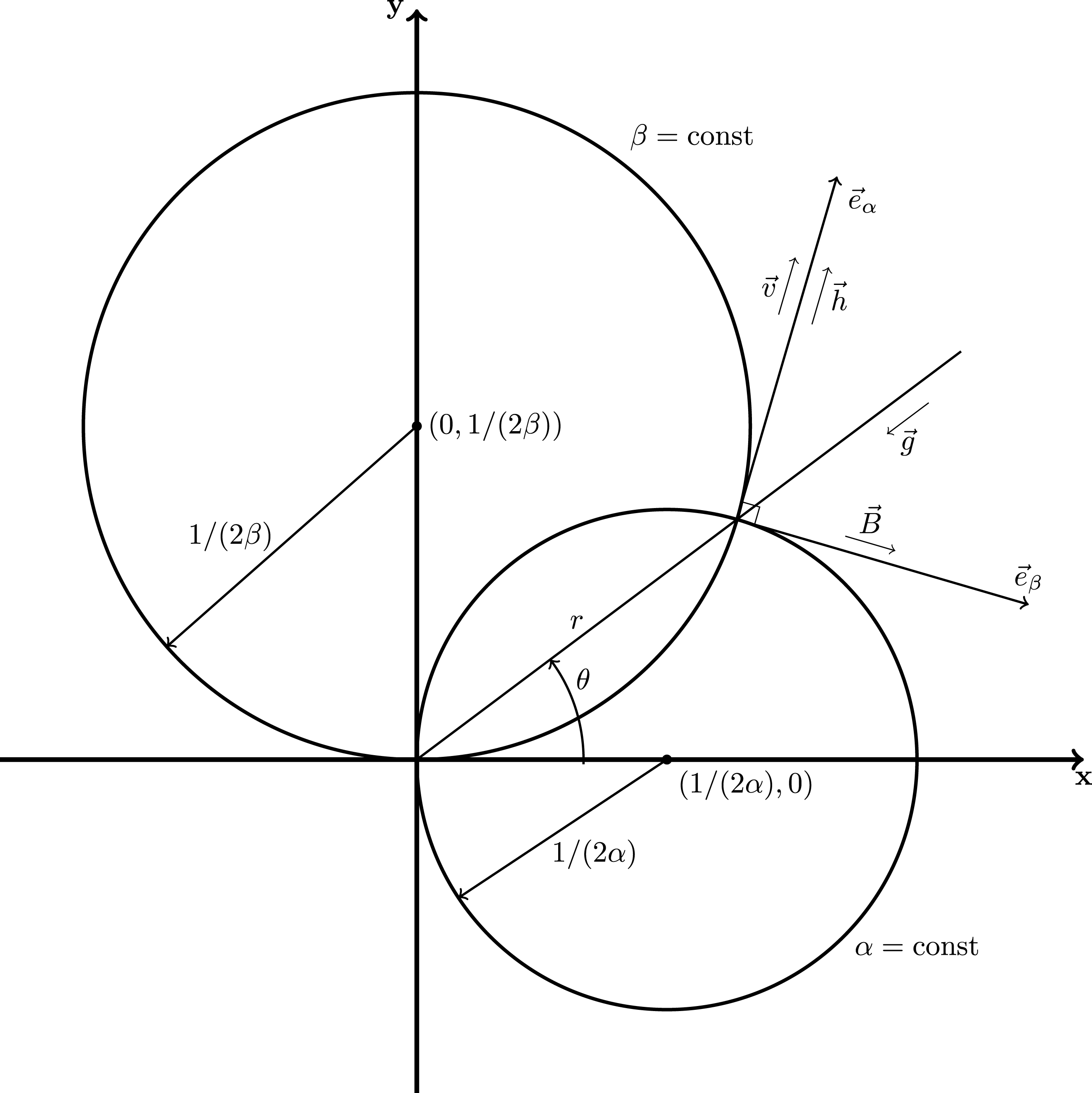
. The transverse, unsteady velocity
 $\boldsymbol{v}$
and magnetic field perturbations
 $\boldsymbol{h}$
are assumed to be parallel and tangent to the coordinate curves
 $\unicode[STIX]{x1D6FD}=\text{const.}$
(according to figure 2),
 $$\begin{eqnarray}\boldsymbol{V}=v(\unicode[STIX]{x1D6FD},t)\boldsymbol{e}_{\unicode[STIX]{x1D6FC}},\quad \boldsymbol{H}=B(\unicode[STIX]{x1D6FD})\boldsymbol{e}_{\unicode[STIX]{x1D6FD}}+h(\unicode[STIX]{x1D6FD},t)\boldsymbol{e}_{\unicode[STIX]{x1D6FC}},\end{eqnarray}$$
and all quantities depend on
 $\unicode[STIX]{x1D6FD}$
, which varies along the curve
 $\unicode[STIX]{x1D6FC}=\text{const}$
. Note that the motion is not incompressible,
 $$\begin{eqnarray}\unicode[STIX]{x1D735}\boldsymbol{\cdot }\boldsymbol{V}=\frac{1}{s^{2}}\frac{\unicode[STIX]{x2202}(sv)}{\unicode[STIX]{x2202}\unicode[STIX]{x1D6FC}}=\frac{v}{s^{2}}\frac{\unicode[STIX]{x2202}s}{\unicode[STIX]{x2202}\unicode[STIX]{x1D6FC}},\end{eqnarray}$$
where, from (2.23),
 $$\begin{eqnarray}\frac{\unicode[STIX]{x2202}s}{\unicode[STIX]{x2202}\unicode[STIX]{x1D6FC}}=-\frac{2\unicode[STIX]{x1D6FC}}{\left(\unicode[STIX]{x1D6FC}^{2}+\unicode[STIX]{x1D6FD}^{2}\right)^{2}}=-2\unicode[STIX]{x1D6FC}s^{2}\end{eqnarray}$$
and consequently equation (2.33) shows that the dilatation is non-zero,
 $$\begin{eqnarray}\unicode[STIX]{x1D735}\boldsymbol{\cdot }\boldsymbol{V}=-2\unicode[STIX]{x1D6FC}v=-2\frac{v}{R};\end{eqnarray}$$
thus there is near incompressibility only for large
 $R$
or small
 $\unicode[STIX]{x1D6FC}$
, i.e. a circle of large radius.
Alfvén wave propagating along a circle with transverse perturbations.

The background magnetic field is divergence free,
 $$\begin{eqnarray}0=\unicode[STIX]{x1D735}\boldsymbol{\cdot }\left(B(\unicode[STIX]{x1D6FD})\boldsymbol{e}_{\unicode[STIX]{x1D6FD}}\right)=\frac{1}{s^{2}}\frac{\unicode[STIX]{x2202}(sB)}{\unicode[STIX]{x2202}\unicode[STIX]{x1D6FD}},\end{eqnarray}$$
if it varies like the inverse of the scale factor,
 $Bs=\text{const.}$
, viz.
 $$\begin{eqnarray}B(r)=\frac{bR^{2}}{s}=\frac{bR^{2}}{r^{2}}=b\sec ^{2}\unicode[STIX]{x1D703},\end{eqnarray}$$
where
 $b$
is the magnetic field strength at radius R,
 $b\equiv B(R)$
. The background magnetic field is, to the level of approximation
 $O(1/R)$
, current free,
 $$\begin{eqnarray}\unicode[STIX]{x1D735}\times (B(\unicode[STIX]{x1D6FD})\boldsymbol{e}_{\unicode[STIX]{x1D6FD}})=0,\end{eqnarray}$$
and hence force free, so that the hydrostatic equilibrium,
 $\unicode[STIX]{x1D735}p=\unicode[STIX]{x1D70C}\boldsymbol{g}$
, applies to the mean state pressure
 $p$
, mass density
 $\unicode[STIX]{x1D70C}$
and gravity
 $\boldsymbol{g}$
, the latter with polar symmetry,
 $$\begin{eqnarray}\boldsymbol{g}=-g_{0}\frac{R}{r}\boldsymbol{e}_{r},\end{eqnarray}$$
where
 $g_{0}$
is the magnitude of the gravity field at radius
 $R$
, that is,
 $g_{0}=|\boldsymbol{g}(R)|$
. Although a uniform magnetic field,
 $\boldsymbol{B}=\text{const.}$
, would be exactly current free, it would not be divergence free and thus it is excluded from the present analysis.
In the case of an incompressible fluid, the density is constant (it does not vary with the radius) and therefore we assume
 $\unicode[STIX]{x1D70C}=\text{const.}\equiv \unicode[STIX]{x1D70C}_{0}$
. In this case, the hydrostatic equilibrium implies
 $$\begin{eqnarray}\frac{\text{d}p}{\text{d}r}=-\unicode[STIX]{x1D70C}_{0}g_{0}\frac{R}{r}.\end{eqnarray}$$
The pressure profile is then given by
 $$\begin{eqnarray}p(r)=p_{0}-\unicode[STIX]{x1D70C}_{0}g_{0}R\log \left(\frac{r}{R}\right),\end{eqnarray}$$
where
 $p_{0}$
is the pressure at radius
 $r=R$
, that is,
 $p_{0}=p(R)$
. The Alfvén speed, defined as
 $$\begin{eqnarray}A=B\sqrt{\frac{1}{\unicode[STIX]{x1D707}\unicode[STIX]{x1D70C}}}\end{eqnarray}$$
using the International System (SI) of units convention, where
 $\unicode[STIX]{x1D707}$
is the magnetic permeability and
 $\unicode[STIX]{x1D70C}$
is the mass density, is given, according to (2.37), by
 $$\begin{eqnarray}A(r)=\frac{aR^{2}}{s}=\frac{aR^{2}}{r^{2}}=a\sec ^{2}\unicode[STIX]{x1D703},\end{eqnarray}$$
where
 $a$
is the Alfvén speed at radius
 $r=R$
and therefore
 $a\equiv b\sqrt{1/\left(\unicode[STIX]{x1D707}\unicode[STIX]{x1D70C}_{0}\right)}\equiv A(R)$
.
In the case of a perfect gas of constant
 $R_{\mathit{g}}$
, at temperature
 $T$
, with molar mass
 $M$
, the equation of state
 $$\begin{eqnarray}p=\frac{\unicode[STIX]{x1D70C}R_{\mathit{g}}T}{M}\end{eqnarray}$$
may be substituted in the condition of hydrostatic equilibrium with
 $$\begin{eqnarray}\unicode[STIX]{x1D735}(\log p)=\frac{\unicode[STIX]{x1D70C}\boldsymbol{g}}{p}=\frac{M\boldsymbol{g}}{R_{\mathit{g}}T},\end{eqnarray}$$
and in isothermal conditions,
 $T=\text{const.}\equiv T_{0}$
, with
 $$\begin{eqnarray}\frac{\text{d}(\log p)}{\text{d}r}=-\frac{Mg_{0}}{R_{\mathit{g}}T_{0}}\frac{R}{r},\end{eqnarray}$$
the pressure profile is a polytropic,
 $$\begin{eqnarray}\frac{\unicode[STIX]{x1D70C}(r)}{\unicode[STIX]{x1D70C}_{0}}=\frac{p(r)}{p_{0}}=\left(\frac{r}{R}\right)^{-\unicode[STIX]{x1D717}},\end{eqnarray}$$
whose index
 $\unicode[STIX]{x1D717}$
is given by
 $\unicode[STIX]{x1D717}\equiv g_{0}MR/\left(R_{\mathit{g}}T_{0}\right)$
where the subscript
 $0$
refers to quantities at radius
 $r=R$
. In this case,
 $\unicode[STIX]{x1D70C}_{0}$
is the density only at
 $r=R$
(the density depends on the radius) while
 $p_{0}$
continues to be the value at the same location. Using
 $R_{\mathit{g}}=8.31~\text{J}~\text{K}^{-1}~\text{mol}^{-1}$
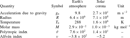
for the ideal gas constant, the polytropic index can be calculated for the atmosphere of the Earth and the end of the solar corona, whose values are indicated in table 1. The values of the temperature and the radius for solar corona are established for the location where the solar wind emerges, in other words, where a stream of particles starts to travel outward to form the heliosphere (figure 1 of Campos Reference Campos1998; Foukal Reference Foukal1990). The solar corona is constituted of ionised hydrogen and therefore its molar mass is
 $1.0\times 10^{-3}~\text{kg}~\text{mol}^{-1}$
. As the values correspond to the height approximately equal to 1 % of the solar radius, the value of the gravitational acceleration is almost the same as at the solar surface. The exponent
 $\unicode[STIX]{x1D708}$
applies to the Alfvén speed (2.42), and substituting (2.37) and (2.47) leads to
 $$\begin{eqnarray}A=a\left(\frac{r}{R}\right)^{-\unicode[STIX]{x1D708}}=a\sec ^{\unicode[STIX]{x1D708}}\unicode[STIX]{x1D703}=a\left(\frac{R^{2}}{s}\right)^{\unicode[STIX]{x1D708}/2},\end{eqnarray}$$
with
 $\unicode[STIX]{x1D708}\equiv 2-\unicode[STIX]{x1D717}/2$
. Comparing (2.48) with (2.43) it follows that
 $\unicode[STIX]{x1D708}=2$
for an incompressible fluid.
Values of several quantities for the atmosphere of the Earth and the solar corona.

3 Alfvén wave equation and extended hypergeometric function
The Alfvén wave equation for propagation along a dipolar magnetic field (see § 3.1) can be solved in terms of Gaussian hypergeometric functions in the limit of zero frequency (see § 3.2) and otherwise requires the solution of an extended Gaussian hypergeometric differential equation (see § 3.3).
The case of zero frequency is considered because it leads to a closed form solution in terms of Gaussian hypergeometric functions. This serves as the stepping stone to the more general case of non-zero frequency that leads to the extended Gaussian hypergeometric differential equation and also has power series solutions with a less simple three-term recurrence formula for the coefficients.
3.1 Alfvén wave equation and polarisation relation
The equations of magnetohydrodynamics, in conformal coordinates, for the case (3.32) read (see Campos & Gil Reference Campos and Gil1995, § 4)
 $$\begin{eqnarray}\displaystyle & \displaystyle s{\dot{h}}=(Bv)^{\prime }, & \displaystyle\end{eqnarray}$$
 $$\begin{eqnarray}\displaystyle & \displaystyle s^{2}\dot{v}=\frac{B}{\unicode[STIX]{x1D707}\unicode[STIX]{x1D70C}}(sh)^{\prime }, & \displaystyle\end{eqnarray}$$
 $t$
and dipolar coordinate
 $\unicode[STIX]{x1D6FD}$
, that is,
 ${\dot{f}}\equiv \unicode[STIX]{x2202}f/\unicode[STIX]{x2202}t$
and
 $f^{\prime }\equiv \unicode[STIX]{x2202}f/\unicode[STIX]{x2202}\unicode[STIX]{x1D6FD}$
. The Alfvén speed (2.42) is introduced in (3.1b
) leading to
 $$\begin{eqnarray}s^{2}\dot{v}=\frac{A^{2}}{B}(sh)^{\prime }.\end{eqnarray}$$
It is possible to eliminate between (3.1a ) and (3.2) either for the velocity (3.3a ) or for the magnetic field perturbations (3.3b ),
 $$\begin{eqnarray}\displaystyle & \displaystyle s^{2}\ddot{v}=\frac{A^{2}}{B}(Bv)^{\prime \prime }, & \displaystyle\end{eqnarray}$$
 $$\begin{eqnarray}\displaystyle & \displaystyle s\ddot{h}=\left[\left(\frac{A}{s}\right)^{2}(sh)^{\prime }\right]^{\prime }. & \displaystyle\end{eqnarray}$$
 $$\begin{eqnarray}\displaystyle & \displaystyle v(\unicode[STIX]{x1D6FD};t)\equiv \int _{-\infty }^{+\infty }V(\unicode[STIX]{x1D6FD};\unicode[STIX]{x1D714})\text{e}^{-\text{i}\unicode[STIX]{x1D714}t}~\text{d}\unicode[STIX]{x1D714}, & \displaystyle\end{eqnarray}$$
 $$\begin{eqnarray}\displaystyle & \displaystyle h(\unicode[STIX]{x1D6FD};t)\equiv \int _{-\infty }^{+\infty }H(\unicode[STIX]{x1D6FD};\unicode[STIX]{x1D714})\text{e}^{-\text{i}\unicode[STIX]{x1D714}t}~\text{d}\unicode[STIX]{x1D714}, & \displaystyle\end{eqnarray}$$
 $V$
and
 $H$
denote respectively the velocity and magnetic field perturbations spectra, for a wave of frequency
 $\unicode[STIX]{x1D714}$
, at position
 $\unicode[STIX]{x1D6FD}$
. Substituting (3.4a
) and (3.4b
) in the Alfvén wave equations for the velocity (3.3a
) and magnetic field perturbations (3.3b
) respectively, these lead to
 $$\begin{eqnarray}\displaystyle & \displaystyle V^{\prime \prime }+2\left(\frac{B^{\prime }}{B}\right)V^{\prime }+\left[\left(\frac{\unicode[STIX]{x1D714}s}{A}\right)^{2}+\frac{B^{\prime \prime }}{B}\right]V=0, & \displaystyle\end{eqnarray}$$
 $$\begin{eqnarray}\displaystyle & \displaystyle H^{\prime \prime }+2\left(\frac{A^{\prime }}{A}\right)H^{\prime }+\left[\left(\frac{\unicode[STIX]{x1D714}s}{A}\right)^{2}+\frac{s}{A^{2}}\left(\frac{A^{2}s^{\prime }}{s^{2}}\right)^{\prime }\right]H=0, & \displaystyle\end{eqnarray}$$
It is sufficient to solve one of the previous wave equations, e.g. the simplest, because once one of
 $V$
or
 $H$
is known, the other can be determined from the polarisation relations,
 $$\begin{eqnarray}\displaystyle & \displaystyle H=\frac{\text{i}}{\unicode[STIX]{x1D714}s}(BV)^{\prime }, & \displaystyle\end{eqnarray}$$
 $$\begin{eqnarray}\displaystyle & \displaystyle V=\frac{\text{i}A^{2}}{\unicode[STIX]{x1D714}s^{2}B}(sH)^{\prime }, & \displaystyle\end{eqnarray}$$
 $$\begin{eqnarray}G(\unicode[STIX]{x1D6FD};\unicode[STIX]{x1D714})\equiv s(\unicode[STIX]{x1D6FD})H(\unicode[STIX]{x1D6FD};\unicode[STIX]{x1D714}),\end{eqnarray}$$
which satisfies a simpler wave equation, starting from (3.3b ),
 $$\begin{eqnarray}0=\unicode[STIX]{x1D714}^{2}G+\left[\left(\frac{A}{s}\right)^{2}G^{\prime }\right]^{\prime },\end{eqnarray}$$
and that may be re-written in the following form
 $$\begin{eqnarray}G^{\prime \prime }+2\left[\log \left(\frac{A}{s}\right)\right]^{\prime }G^{\prime }+\left(\frac{\unicode[STIX]{x1D714}s}{A}\right)^{2}G=0.\end{eqnarray}$$
This equation has only one non-constant coefficient, in contrast with the two equations (3.5), that have several non-constant coefficients. This coefficient is evaluated from (2.29) and (2.48),
 $$\begin{eqnarray}\frac{A}{s}=aR^{\unicode[STIX]{x1D708}}s^{-1-\unicode[STIX]{x1D708}/2}=\frac{a}{R^{2}}\cos ^{-\unicode[STIX]{x1D708}-2}\unicode[STIX]{x1D703},\end{eqnarray}$$
and the derivative with regard to
 $\unicode[STIX]{x1D6FD}$
is replaced, using (2.30), by a derivative with regard to
 $\unicode[STIX]{x1D703}$
,
 $$\begin{eqnarray}\left[\log \left(\frac{A}{s}\right)\right]^{\prime }=R\cos ^{2}\unicode[STIX]{x1D703}\frac{\text{d}}{\text{d}\unicode[STIX]{x1D703}}[(-\unicode[STIX]{x1D708}-2)\log (\cos \unicode[STIX]{x1D703})]=R(\unicode[STIX]{x1D708}+2)\cos \unicode[STIX]{x1D703}\sin \unicode[STIX]{x1D703}.\end{eqnarray}$$
Substituting the last two equations in (3.9), viz.
 $$\begin{eqnarray}G^{\prime \prime }+2R(\unicode[STIX]{x1D708}+2)\cos \unicode[STIX]{x1D703}\sin \unicode[STIX]{x1D703}G^{\prime }+\left(\frac{\unicode[STIX]{x1D714}R^{2}}{a}\right)^{2}\cos ^{2\unicode[STIX]{x1D708}+4}\unicode[STIX]{x1D703}G=0,\end{eqnarray}$$
it is appropriate to replace the derivatives with regard to
 $\unicode[STIX]{x1D6FD}$
, e.g.
 $G^{\prime \prime }\equiv \text{d}^{2}G/\text{d}\unicode[STIX]{x1D6FD}^{2}$
, by derivatives with regard to
 $\unicode[STIX]{x1D703}$
, e.g.
 $\text{d}^{2}\unicode[STIX]{x1D6F7}/\text{d}\unicode[STIX]{x1D703}^{2}\equiv \unicode[STIX]{x1D6F7}^{\prime \prime }$
, noting that
 $$\begin{eqnarray}\unicode[STIX]{x1D6F7}(\unicode[STIX]{x1D703};\unicode[STIX]{x1D6FA})\equiv G(\unicode[STIX]{x1D6FD};\unicode[STIX]{x1D714}),\end{eqnarray}$$
and using (2.30), viz.
 $$\begin{eqnarray}\cos ^{2}\unicode[STIX]{x1D703}\unicode[STIX]{x1D6F7}^{\prime \prime }+2(\unicode[STIX]{x1D708}+1)\cos \unicode[STIX]{x1D703}\sin \unicode[STIX]{x1D703}\unicode[STIX]{x1D6F7}^{\prime }+\unicode[STIX]{x1D6FA}^{2}\cos ^{2\unicode[STIX]{x1D708}+2}\unicode[STIX]{x1D703}\unicode[STIX]{x1D6F7}=0;\end{eqnarray}$$
the Alfvén wave equation (3.14) involves only one parameter, namely, the dimensionless frequency
 $\unicode[STIX]{x1D6FA}\equiv \unicode[STIX]{x1D714}R/a$
.
The Alfvén wave equation (3.14) has coefficients which are trigonometric functions of
 $\unicode[STIX]{x1D703}$
in the range
 $0\leqslant \unicode[STIX]{x1D703}\leqslant 2\unicode[STIX]{x03C0}$
, and these can be transformed to polynomial coefficients, via the change of independent variable,
 $$\begin{eqnarray}\unicode[STIX]{x1D701}=\cos ^{2}\unicode[STIX]{x1D703},\quad \unicode[STIX]{x1D6F9}(\unicode[STIX]{x1D701};\unicode[STIX]{x1D6FA})=\unicode[STIX]{x1D6F7}(\unicode[STIX]{x1D703};\unicode[STIX]{x1D6FA}),\end{eqnarray}$$
where
 $0\leqslant \unicode[STIX]{x1D701}\leqslant 1$
,
 $$\begin{eqnarray}4\unicode[STIX]{x1D701}^{2}(1-\unicode[STIX]{x1D701})\unicode[STIX]{x1D6F9}^{\prime \prime }-2\unicode[STIX]{x1D701}[1+2\unicode[STIX]{x1D708}(1-\unicode[STIX]{x1D701})]\unicode[STIX]{x1D6F9}^{\prime }+\unicode[STIX]{x1D6FA}^{2}\unicode[STIX]{x1D701}^{\unicode[STIX]{x1D708}+1}\unicode[STIX]{x1D6F9}=0.\end{eqnarray}$$
The degree of the polynomial coefficients of the highest derivative
 $\unicode[STIX]{x1D6F9}^{\prime \prime }$
, viz. three in (3.16), can be depressed to two via the change of independent variable,
 $$\begin{eqnarray}\unicode[STIX]{x1D6F9}(\unicode[STIX]{x1D701};\unicode[STIX]{x1D6FA})=\unicode[STIX]{x1D701}^{\unicode[STIX]{x1D70E}}Q(\unicode[STIX]{x1D701};\unicode[STIX]{x1D6FA}),\end{eqnarray}$$
where the constant
 $\unicode[STIX]{x1D70E}$
can be chosen at will, e.g. so that
 $$\begin{eqnarray}\displaystyle & & \displaystyle 4(1-\unicode[STIX]{x1D701})\unicode[STIX]{x1D701}^{2}Q^{\prime \prime }-2[1-2(2\unicode[STIX]{x1D70E}-\unicode[STIX]{x1D708})(1-\unicode[STIX]{x1D701})]\unicode[STIX]{x1D701}Q^{\prime }\nonumber\\ \displaystyle & & \displaystyle \quad \text{}+\,\left[\unicode[STIX]{x1D6FA}^{2}\unicode[STIX]{x1D701}^{1+\unicode[STIX]{x1D708}}-4\unicode[STIX]{x1D70E}\unicode[STIX]{x1D701}(\unicode[STIX]{x1D70E}-1-\unicode[STIX]{x1D708})+2\unicode[STIX]{x1D70E}(2\unicode[STIX]{x1D70E}-3-2\unicode[STIX]{x1D708})\right]Q=0\end{eqnarray}$$
can be divided through by
 $\unicode[STIX]{x1D701}$
. This is the case if the term in the last curved brackets vanishes,
 $$\begin{eqnarray}\unicode[STIX]{x1D70E}={\textstyle \frac{3}{2}}+\unicode[STIX]{x1D708},\quad \unicode[STIX]{x1D6F9}(\unicode[STIX]{x1D701};\unicode[STIX]{x1D6FA})=\unicode[STIX]{x1D701}^{\unicode[STIX]{x1D708}+3/2}Q(\unicode[STIX]{x1D701};\unicode[STIX]{x1D6FA}),\end{eqnarray}$$
in which case the wave equation simplifies to
 $$\begin{eqnarray}4(1-\unicode[STIX]{x1D701})\unicode[STIX]{x1D701}Q^{\prime \prime }-2[1-2(3+\unicode[STIX]{x1D708})(1-\unicode[STIX]{x1D701})]Q^{\prime }+\left(\unicode[STIX]{x1D6FA}^{2}\unicode[STIX]{x1D701}^{\unicode[STIX]{x1D708}}-3-2\unicode[STIX]{x1D708}\right)Q=0.\end{eqnarray}$$
A dipolar magnetic field is an approximate first-order representation of the Earth’s field, remembering that
 $\unicode[STIX]{x1D708}$
is given by
 $\unicode[STIX]{x1D708}\equiv 2-\unicode[STIX]{x1D717}/2$
, with
 $\unicode[STIX]{x1D717}\equiv g_{0}MR/\left(R_{\mathit{g}}T_{0}\right)$
, in the case of Alfvén waves in the ionosphere, which is gaseous, or
 $\unicode[STIX]{x1D708}=2$
in (2.43) for Alfvén waves in the molten core, which is incompressible. This application is limited by our consideration of a planar rather than spherical problem, and neglect of rotation, a non-central symmetry. In the case of an incompressible fluid, e.g. a liquid, the Alfvén wave equation (3.20) simplifies to
 $$\begin{eqnarray}\unicode[STIX]{x1D708}=2:\quad 4(1-\unicode[STIX]{x1D701})\unicode[STIX]{x1D701}Q^{\prime \prime }+2(9-10\unicode[STIX]{x1D701})Q^{\prime }+\left(\unicode[STIX]{x1D6FA}^{2}\unicode[STIX]{x1D701}^{2}-7\right)Q=0.\end{eqnarray}$$
The differential equation (3.21) reduces to the Gaussian hypergeometric type, leading to an analytic closed form solution, in the limit of zero frequency, corresponding to the steady magnetic field (see § 3.2) in contrast with the case of the unsteady magnetic field for Alfvén waves when a power series solution also exists (see § 3.3) with a three-term instead of a two-term recurrence formula for the coefficients.
3.2 Limit of zero frequency and hypergeometric functions
In the limiting case of zero frequency, i.e. quasi-steady field, the differential equation (3.21) simplifies to
 $$\begin{eqnarray}\unicode[STIX]{x1D6FA}=0:\quad (1-\unicode[STIX]{x1D701})\unicode[STIX]{x1D701}Q^{\prime \prime }+\left({\textstyle \frac{9}{2}}-5\unicode[STIX]{x1D701}\right)Q^{\prime }-{\textstyle \frac{7}{4}}Q=0,\end{eqnarray}$$
which is of the Gaussian hypergeometric type,
 $$\begin{eqnarray}(1-\unicode[STIX]{x1D701})\unicode[STIX]{x1D701}Q^{\prime \prime }+[\unicode[STIX]{x1D6FE}-(\unicode[STIX]{x1D6FC}+\unicode[STIX]{x1D6FD}+1)\unicode[STIX]{x1D701}]Q^{\prime }-\unicode[STIX]{x1D6FC}\unicode[STIX]{x1D6FD}Q=0,\end{eqnarray}$$
with parameters satisfying
 $$\begin{eqnarray}\unicode[STIX]{x1D6FE}={\textstyle \frac{9}{2}},\quad \unicode[STIX]{x1D6FC}+\unicode[STIX]{x1D6FD}=4,\quad \unicode[STIX]{x1D6FC}\unicode[STIX]{x1D6FD}={\textstyle \frac{7}{4}},\end{eqnarray}$$
leading to
 $\unicode[STIX]{x1D6FC}=1/2$
and
 $\unicode[STIX]{x1D6FD}=7/2$
. The general integral of the Gaussian hypergeometric differential equation (3.22) is
 $$\begin{eqnarray}\displaystyle Q(\unicode[STIX]{x1D701};0)=c_{1}F(\unicode[STIX]{x1D6FC},\unicode[STIX]{x1D6FD};\unicode[STIX]{x1D6FE};\unicode[STIX]{x1D701})+c_{2}\unicode[STIX]{x1D701}^{1-\unicode[STIX]{x1D6FE}}F(1+\unicode[STIX]{x1D6FC}-\unicode[STIX]{x1D6FE},1+\unicode[STIX]{x1D6FD}-\unicode[STIX]{x1D6FE};2-\unicode[STIX]{x1D6FE};\unicode[STIX]{x1D701}) & & \displaystyle\end{eqnarray}$$
provided that
 $\unicode[STIX]{x1D6FE}$
is not an integer while
 $c_{1}$
and
 $c_{2}$
are arbitrary constants of integration. In the present case, the general integral is
 $$\begin{eqnarray}Q(\unicode[STIX]{x1D701};0)=c_{1}F\left({\textstyle \frac{1}{2}},{\textstyle \frac{7}{2}};{\textstyle \frac{9}{2}};\unicode[STIX]{x1D701}\right)+c_{2}\unicode[STIX]{x1D701}^{-7/2}F\left(-3,0;-{\textstyle \frac{5}{2}};\unicode[STIX]{x1D701}\right).\end{eqnarray}$$
Recalling the expressions (2.29), (3.7), (3.13), (3.15) and (3.19) the magnetic field perturbation is
 $$\begin{eqnarray}\displaystyle H(\unicode[STIX]{x1D6FD};\unicode[STIX]{x1D714}) & = & \displaystyle \frac{G(\unicode[STIX]{x1D6FD};\unicode[STIX]{x1D714})}{s}=\frac{\unicode[STIX]{x1D6F7}(\unicode[STIX]{x1D703};\unicode[STIX]{x1D6FA})}{R^{2}\cos ^{2}\unicode[STIX]{x1D703}}=\frac{\unicode[STIX]{x1D6F9}(\cos ^{2}\unicode[STIX]{x1D703};\unicode[STIX]{x1D6FA})}{R^{2}\cos ^{2}\unicode[STIX]{x1D703}}\nonumber\\ \displaystyle & = & \displaystyle \frac{\cos ^{2\unicode[STIX]{x1D708}+1}\unicode[STIX]{x1D703}\,Q(\cos ^{2}\unicode[STIX]{x1D703};\unicode[STIX]{x1D6FA})}{R^{2}}.\end{eqnarray}$$
A magnetic field decaying like
 $O(1/R)$
would not satisfy the conservation of magnetic flux across a sphere of radius
 $R$
, unless the angular dependence would lead to a zero integral over the surface of the sphere. All the solutions for the magnetic field in this paper decay like
 $O(1/R^{2})$
, implying that the magnetic flux crossing a sphere of radius
 $R$
is constant for any angular dependence, and thus that Gauss’ law for magnetism is met.
A magnetic field perturbation spectrum
 $h(\unicode[STIX]{x1D703};\unicode[STIX]{x1D6FA})$
is introduced that does not depend on the radius
 $R$
of the circle and depends only on the angle
 $\unicode[STIX]{x1D703}$
along the circle; in the case
 $\unicode[STIX]{x1D708}=2$
and
 $\unicode[STIX]{x1D6FA}=0$
, it simplifies to
 $$\begin{eqnarray}h(\unicode[STIX]{x1D703};0)\equiv b^{-1}H(\unicode[STIX]{x1D703};0)=C_{1}\cos ^{5}\unicode[STIX]{x1D703}F\left({\textstyle \frac{1}{2}},{\textstyle \frac{7}{2}};{\textstyle \frac{9}{2}};\cos ^{2}\unicode[STIX]{x1D703}\right)+C_{2}\sec ^{2}\unicode[STIX]{x1D703}F\left(-3,0;-{\textstyle \frac{5}{2}};\cos ^{2}\unicode[STIX]{x1D703}\right)\!,\end{eqnarray}$$
where in the second equality the constants
 $b^{-1}$
and
 $R^{-2}$
were incorporated in the constants of integration, that is,
 $C_{1}\equiv b^{-1}R^{-2}c_{1}$
and
 $C_{2}\equiv b^{-1}R^{-2}c_{2}$
. The second hypergeometric function on the right-hand side of (3.28), knowing that
 $$\begin{eqnarray}\displaystyle F(\unicode[STIX]{x1D6FC},\unicode[STIX]{x1D6FD};\unicode[STIX]{x1D6FE};\unicode[STIX]{x1D701}) & = & \displaystyle 1+\frac{\unicode[STIX]{x1D6FC}\unicode[STIX]{x1D6FD}}{1!\unicode[STIX]{x1D6FE}}\unicode[STIX]{x1D701}^{1}+\frac{\unicode[STIX]{x1D6FC}(\unicode[STIX]{x1D6FC}+1)\unicode[STIX]{x1D6FD}(\unicode[STIX]{x1D6FD}+1)}{2!\unicode[STIX]{x1D6FE}(\unicode[STIX]{x1D6FE}+1)}\unicode[STIX]{x1D701}^{2}+\cdots\end{eqnarray}$$
 $$\begin{eqnarray}\displaystyle & & \displaystyle +\,\frac{\unicode[STIX]{x1D6FC}(\unicode[STIX]{x1D6FC}+1)\cdots (\unicode[STIX]{x1D6FC}+n-1)\unicode[STIX]{x1D6FD}(\unicode[STIX]{x1D6FD}+1)\cdots (\unicode[STIX]{x1D6FD}+n-1)}{n!\unicode[STIX]{x1D6FE}(\unicode[STIX]{x1D6FE}+1)\cdots (\unicode[STIX]{x1D6FE}+n-1)}\unicode[STIX]{x1D701}^{n}+\cdots \,,\qquad \quad\end{eqnarray}$$
reduces to unity because
 $\unicode[STIX]{x1D6FD}$
is zero,
 $$\begin{eqnarray}F\left(-3,0;-{\textstyle \frac{5}{2}};\cos ^{2}\unicode[STIX]{x1D703}\right)=1,\end{eqnarray}$$
implying that
 $\unicode[STIX]{x1D701}^{-7/2}$
is a solution of (3.22), as can be checked directly. It can be noted in passing that, since a solution
 $\unicode[STIX]{x1D701}^{-7/2}$
is known, another solution can be obtained (Forsyth Reference Forsyth1956), viz.
 $$\begin{eqnarray}\unicode[STIX]{x1D701}^{-7/2}\int (1-\unicode[STIX]{x1D701})^{-1/2}\unicode[STIX]{x1D701}^{5/2}~\text{d}\unicode[STIX]{x1D701},\end{eqnarray}$$
which must be a linear combination of the two in (3.26). These two algebraic solutions would avoid the use of hypergeometric functions, whereas the latter are more closely linked to the case of non-zero frequency and Alfvén waves. However, the factor
 $\sec ^{2}\unicode[STIX]{x1D703}$
is singular for
 $\unicode[STIX]{x1D703}=\pm \unicode[STIX]{x03C0}/2$
and a finite magnetic field requires
 $C_{2}=0$
, simplifying (3.28) to
 $$\begin{eqnarray}h(\unicode[STIX]{x1D703};0)=C_{1}\cos ^{5}\unicode[STIX]{x1D703}F\left({\textstyle \frac{1}{2}},{\textstyle \frac{7}{2}};{\textstyle \frac{9}{2}};\cos ^{2}\unicode[STIX]{x1D703}\right)\end{eqnarray}$$
that vanishes for
 $\unicode[STIX]{x1D703}=\pm \unicode[STIX]{x03C0}/2$
. The hypergeometric series in the first term is finite for
 $|\!\cos \unicode[STIX]{x1D703}|<1$
. Since
 $\unicode[STIX]{x1D6FE}-\unicode[STIX]{x1D6FC}-\unicode[STIX]{x1D6FD}=1/2$
the hypergeometric series converges (Bromwich Reference Bromwich1926; Campos Reference Campos1988a
; Knopp Reference Knopp1990) on its radius of convergence
 $|\!\cos \unicode[STIX]{x1D703}|=1$
or
 $\unicode[STIX]{x1D703}=0,\unicode[STIX]{x03C0}$
. Using the property
 $$\begin{eqnarray}F(\unicode[STIX]{x1D6FC},\unicode[STIX]{x1D6FD};\unicode[STIX]{x1D6FE};1)=\frac{\unicode[STIX]{x1D6E4}(\unicode[STIX]{x1D6FE})\unicode[STIX]{x1D6E4}(\unicode[STIX]{x1D6FE}-\unicode[STIX]{x1D6FC}-\unicode[STIX]{x1D6FD})}{\unicode[STIX]{x1D6E4}(\unicode[STIX]{x1D6FE}-\unicode[STIX]{x1D6FC})\unicode[STIX]{x1D6E4}(\unicode[STIX]{x1D6FE}-\unicode[STIX]{x1D6FD})},\end{eqnarray}$$
where
 $\unicode[STIX]{x1D6E4}$
is the gamma function (Abramowitz & Stegun Reference Abramowitz and Stegun1965) specifies the constant of integration
 $C_{1}$
from the magnetic field at
 $\unicode[STIX]{x1D703}=0$
,
 $$\begin{eqnarray}h(0;0)=C_{1}F\left(\frac{1}{2},\frac{7}{2};\frac{9}{2};1\right)=C_{1}\frac{\unicode[STIX]{x1D6E4}(9/2)\unicode[STIX]{x1D6E4}(1/2)}{\unicode[STIX]{x1D6E4}(4)\unicode[STIX]{x1D6E4}(1)}=C_{1}\frac{\frac{7}{2}\frac{5}{2}\frac{3}{2}\left[\unicode[STIX]{x1D6E4}\left(\frac{1}{2}\right)\right]^{2}}{3!}=\frac{35\unicode[STIX]{x03C0}}{16}C_{1},\end{eqnarray}$$
using in the last equality
 $\unicode[STIX]{x1D6E4}(1/2)=\sqrt{\unicode[STIX]{x03C0}}$
(Copson Reference Copson1935; Whittaker & Watson Reference Whittaker and Watson1996). Thus the magnetic field in the incompressible case
 $\unicode[STIX]{x1D708}=2$
, for zero frequency
 $\unicode[STIX]{x1D6FA}=0$
, simplifies from (3.28) to (3.33) to be bounded for all
 $0\leqslant \unicode[STIX]{x1D703}\leqslant \unicode[STIX]{x03C0}$
with the constant
 $C_{1}$
determined by the value (3.35) at
 $\unicode[STIX]{x1D703}=0$
, so that
 $$\begin{eqnarray}h(\unicode[STIX]{x1D703};0)=h(0;0)\frac{16}{35\unicode[STIX]{x03C0}}\cos ^{5}\unicode[STIX]{x1D703}F\left(\frac{1}{2},\frac{7}{2};\frac{9}{2};\cos ^{2}\unicode[STIX]{x1D703}\right).\end{eqnarray}$$
This closed form solution shares the angular dependence of the leading term
 $\cos ^{5}\unicode[STIX]{x1D703}$
with the more interesting case of non-zero frequency, leading to an extension of the Gaussian hypergeometric differential equation.
3.3 Non-zero frequency and extended hypergeometric equations
In the more interesting case of non-zero frequency, the wave equation (3.21) is of the extended Gaussian hypergeometric type, so-called because: (I)
 $\unicode[STIX]{x1D701}=0,1$
are regular singularities, as for the original Gaussian hypergeometric equation (3.22); (II) the point-at-infinity
 $\unicode[STIX]{x1D701}=\infty$
is a regular singularity for the latter, and an irregular singularity for the former, in this case of degree two. Since
 $\unicode[STIX]{x1D701}=0$
is a regular singularity, solutions exist, with radius of convergence unity, limited by the nearest singularity, in terms of a Frobenius–Fuchs series,
 $$\begin{eqnarray}|\unicode[STIX]{x1D701}|<1:\quad \overline{Q}(\unicode[STIX]{x1D701};\unicode[STIX]{x1D6FA})\equiv b^{-1}R^{-2}Q(\unicode[STIX]{x1D701};\unicode[STIX]{x1D6FA})=\mathop{\sum }_{n=0}^{\infty }c_{n}(\unicode[STIX]{x1D712})\unicode[STIX]{x1D701}^{n+\unicode[STIX]{x1D712}},\end{eqnarray}$$
with index
 $\unicode[STIX]{x1D712}$
and the recurrence formula for the coefficients
 $c_{n}(\unicode[STIX]{x1D712})$
to be determined. Substitution of (3.37) in (3.21) leads to the recurrence formula for the coefficients
 $$\begin{eqnarray}(n+\unicode[STIX]{x1D712}+1)\left(n+\unicode[STIX]{x1D712}+\frac{9}{2}\right)c_{n+1}(\unicode[STIX]{x1D712})=\left[(n+\unicode[STIX]{x1D712})(n+\unicode[STIX]{x1D712}+4)+\frac{7}{4}\right]c_{n}(\unicode[STIX]{x1D712})-\left(\frac{\unicode[STIX]{x1D6FA}}{2}\right)^{2}c_{n-2}(\unicode[STIX]{x1D712}).\end{eqnarray}$$
In the case of zero frequency,
 $\unicode[STIX]{x1D6FA}=0$
, this would reduce to the simple recurrence formula for Gaussian hypergeometric functions
 $$\begin{eqnarray}\displaystyle c_{n+1}(\unicode[STIX]{x1D712}) & = & \displaystyle \left[\frac{(n+\unicode[STIX]{x1D712})(n+\unicode[STIX]{x1D712}+4)+7/4}{(n+\unicode[STIX]{x1D712}+1)(n+\unicode[STIX]{x1D712}+9/2)}\right]c_{n}(\unicode[STIX]{x1D712})\nonumber\\ \displaystyle & = & \displaystyle c_{0}(\unicode[STIX]{x1D712})\mathop{\prod }_{m=0}^{n}\left[\frac{(m+\unicode[STIX]{x1D712}+1/2)(m+\unicode[STIX]{x1D712}+7/2)}{(m+\unicode[STIX]{x1D712}+1)(m+\unicode[STIX]{x1D712}+9/2)}\right],\end{eqnarray}$$
in agreement with the values of
 $\unicode[STIX]{x1D6FE}$
,
 $\unicode[STIX]{x1D6FC}$
and
 $\unicode[STIX]{x1D6FD}$
for zero frequency; otherwise, for non-zero frequency
 $\unicode[STIX]{x1D6FA}\neq 0$
, the recurrence relation (3.38) has three terms. Setting
 $n=-1$
yields in both cases the indicial equation
 $$\begin{eqnarray}\unicode[STIX]{x1D712}\left(\unicode[STIX]{x1D712}+{\textstyle \frac{7}{2}}\right)=0,\end{eqnarray}$$
whose roots
 $\unicode[STIX]{x1D712}=0$
and
 $\unicode[STIX]{x1D712}=-7/2$
specify two linearly independent particular integrals, respectively
 $$\begin{eqnarray}\displaystyle & \displaystyle \overline{Q}_{0}(\unicode[STIX]{x1D701};\unicode[STIX]{x1D6FA})\equiv \mathop{\sum }_{n=0}^{\infty }c_{n}(0)\unicode[STIX]{x1D701}^{n}, & \displaystyle\end{eqnarray}$$
 $$\begin{eqnarray}\displaystyle & \displaystyle \overline{Q}_{1}(\unicode[STIX]{x1D701};\unicode[STIX]{x1D6FA})\equiv \mathop{\sum }_{n=0}^{\infty }c_{n}\left(-\frac{7}{2}\right)\unicode[STIX]{x1D701}^{n-7/2}, & \displaystyle\end{eqnarray}$$
 $0<\unicode[STIX]{x1D701}<1$
, is the general integral
 $$\begin{eqnarray}h(\unicode[STIX]{x1D701};\unicode[STIX]{x1D6FA})=\cos ^{5}\unicode[STIX]{x1D703}\overline{Q}_{0}(\unicode[STIX]{x1D701};\unicode[STIX]{x1D6FA})+\cos ^{5}\unicode[STIX]{x1D703}\overline{Q}_{1}(\unicode[STIX]{x1D701};\unicode[STIX]{x1D6FA}).\end{eqnarray}$$
Substituting in (3.27) leads, for
 $0<\unicode[STIX]{x1D703}<\unicode[STIX]{x03C0}$
, to the magnetic field perturbation spectrum
 $$\begin{eqnarray}h(\unicode[STIX]{x1D703};\unicode[STIX]{x1D6FA})=\cos ^{5}\unicode[STIX]{x1D703}\mathop{\sum }_{n=0}^{\infty }c_{n}(0)\cos ^{2n}\unicode[STIX]{x1D703}+\sec ^{2}\unicode[STIX]{x1D703}\mathop{\sum }_{n=0}^{\infty }c_{n}\left(-\frac{7}{2}\right)\cos ^{2n}\unicode[STIX]{x1D703},\end{eqnarray}$$
where the role of arbitrary constants, to be consistent with the zero frequency case, is played by
 $C_{1}\equiv c_{0}(0)$
and
 $C_{2}\equiv c_{0}(-7/2)$
. The second term of the wavefield (3.43) is singular at
 $\unicode[STIX]{x1D703}=\pm \unicode[STIX]{x03C0}/2$
; thus a finite solution over the whole circle
 $0\leqslant \unicode[STIX]{x1D703}\leqslant \unicode[STIX]{x03C0}$
requires
 $C_{2}=0$
.
The first term corresponds to the series (3.41a
) which converges for
 $|\unicode[STIX]{x1D701}|<1$
or
 $\cos ^{2}\unicode[STIX]{x1D703}<1$
or
 $0<\unicode[STIX]{x1D703}<\unicode[STIX]{x03C0}$
, so that the wavefield is finite in this range. The points
 $\unicode[STIX]{x1D703}=0,\unicode[STIX]{x03C0}$
correspond to the boundary of convergence. In order to find out whether the wavefield is finite at
 $\unicode[STIX]{x1D703}=0,\unicode[STIX]{x03C0}$
in the case
 $\unicode[STIX]{x1D6FA}\neq 0$
, as for
 $\unicode[STIX]{x1D6FA}=0$
, it is necessary to determine
 $h(0;\unicode[STIX]{x1D6FA})$
. Since generalisations of the relations (3.34) are not available for extended hypergeometric functions, it is necessary to go back to the differential equation (3.21) and perform the change of variable
 $$\begin{eqnarray}\unicode[STIX]{x1D709}\equiv 1-\unicode[STIX]{x1D701}=\sin ^{2}\unicode[STIX]{x1D703},\quad J(\unicode[STIX]{x1D709};\unicode[STIX]{x1D6FA})=Q(\unicode[STIX]{x1D701};\unicode[STIX]{x1D6FA});\end{eqnarray}$$
this transforms the wave equation (3.21) to
 $$\begin{eqnarray}4\unicode[STIX]{x1D709}(1-\unicode[STIX]{x1D709})J^{\prime \prime }+2(1-10\unicode[STIX]{x1D709})J^{\prime }+\left(\unicode[STIX]{x1D6FA}^{2}\unicode[STIX]{x1D709}^{2}-2\unicode[STIX]{x1D6FA}^{2}\unicode[STIX]{x1D709}+\unicode[STIX]{x1D6FA}^{2}-7\right)J=0.\end{eqnarray}$$
Since
 $\unicode[STIX]{x1D701}=1$
is a regular singularity of (3.21),
 $\unicode[STIX]{x1D709}=0$
is a regular singularity of (3.45), and a solution as a Frobenius–Fuchs series exists
 $$\begin{eqnarray}\overline{J}_{\unicode[STIX]{x1D6F9}}(\unicode[STIX]{x1D709};\unicode[STIX]{x1D6FA})\equiv b^{-1}R^{-2}J_{\unicode[STIX]{x1D6F9}}(\unicode[STIX]{x1D709};\unicode[STIX]{x1D6FA})=\mathop{\sum }_{n=0}^{\infty }d_{n}(\unicode[STIX]{x1D6F9})\unicode[STIX]{x1D709}^{n+\unicode[STIX]{x1D6F9}}.\end{eqnarray}$$
The recurrence formula for the coefficients
 $$\begin{eqnarray}\displaystyle (n+\unicode[STIX]{x1D6F9}+1)\left(n+\unicode[STIX]{x1D6F9}+\frac{1}{2}\right)d_{n+1}(\unicode[STIX]{x1D6F9}) & = & \displaystyle \left[(n+\unicode[STIX]{x1D6F9})(n+\unicode[STIX]{x1D6F9}+4)+\frac{7}{4}-\frac{\unicode[STIX]{x1D6FA}^{2}}{4}\right]d_{n}(\unicode[STIX]{x1D6F9})\nonumber\\ \displaystyle & & \displaystyle \text{}+\frac{\unicode[STIX]{x1D6FA}^{2}}{2}d_{n-1}(\unicode[STIX]{x1D6F9})-\left(\frac{\unicode[STIX]{x1D6FA}}{2}\right)^{2}d_{n-2}(\unicode[STIX]{x1D6F9})\end{eqnarray}$$
leads to the indicial equation
 $$\begin{eqnarray}\unicode[STIX]{x1D6F9}\left(\unicode[STIX]{x1D6F9}-\frac{1}{2}\right)=0,\end{eqnarray}$$
with the roots
 $\unicode[STIX]{x1D6F9}=0,1/2$
. It is clear that the wavefield will be finite
 $\overline{J}_{0}(\unicode[STIX]{x1D709})\sim O(1)$
or vanish
 $\overline{J}_{1/2}(\unicode[STIX]{x1D709})\sim O(\sqrt{\unicode[STIX]{x1D709}})$
at
 $\unicode[STIX]{x1D709}=0$
, i.e. for
 $\unicode[STIX]{x1D703}=0$
and
 $\unicode[STIX]{x1D703}=\unicode[STIX]{x03C0}$
; therefore both of (3.41a
) and (3.41b
), which are linear combinations of
 $\overline{J}_{0}$
and
 $\overline{J}_{1/2}$
, must be finite at
 $\unicode[STIX]{x1D703}=0$
and
 $\unicode[STIX]{x1D703}=\unicode[STIX]{x03C0}$
. As before, the general integral may be written as
 $$\begin{eqnarray}h(\unicode[STIX]{x1D703};\unicode[STIX]{x1D6FA})=\cos ^{5}\unicode[STIX]{x1D703}\left[\mathop{\sum }_{n=0}^{\infty }d_{n}(0)\sin ^{2n}\unicode[STIX]{x1D703}+\sin \unicode[STIX]{x1D703}\mathop{\sum }_{n=0}^{\infty }d_{n}\left(\frac{1}{2}\right)\sin ^{2n}\unicode[STIX]{x1D703}\right]\end{eqnarray}$$
where the arbitrary constants of integration, again to be consistent with the zero frequency case, are now
 $D_{1}\equiv d_{0}(0)$
and
 $D_{2}\equiv d_{0}(1/2)$
. This formula shows that at
 $\unicode[STIX]{x1D703}=0,\unicode[STIX]{x03C0}$
the wavefield is finite because
 $h(0;\unicode[STIX]{x1D6FA})=d_{0}(0)=D_{1}=-h(\unicode[STIX]{x03C0};\unicode[STIX]{x1D6FA})$
.
4 Velocity and magnetic field perturbations
The solution of the Alfvén wave equation (see § 3) leads to series expansions for the velocity and magnetic field perturbations (see § 4.1) which converge rapidly (see § 4.2) and allow plotting of the wavefields.
4.1 Boundary conditions and wave perturbations
The pairs of arbitrary constants
 $C_{1}$
and
 $C_{2}$
are determined by two non-trivial, independent and compatible boundary conditions, e.g. specifying the magnetic field perturbation at two points,
 $$\begin{eqnarray}h(\unicode[STIX]{x1D703}_{1};\unicode[STIX]{x1D6FA})\equiv h_{1}(\unicode[STIX]{x1D6FA}),\quad h_{2}(\unicode[STIX]{x1D703}_{2};\unicode[STIX]{x1D6FA})\equiv h_{2}(\unicode[STIX]{x1D6FA}),\end{eqnarray}$$
or the magnetic field perturbation and its derivative at one point,
 $$\begin{eqnarray}h(\unicode[STIX]{x1D703}_{0};\unicode[STIX]{x1D6FA})\equiv h_{0}(\unicode[STIX]{x1D6FA}),\quad \left.\frac{\text{d}h}{\text{d}\unicode[STIX]{x1D703}}\right|_{\unicode[STIX]{x1D703}=\unicode[STIX]{x1D703}_{0}}\equiv h_{0}^{\prime }(\unicode[STIX]{x1D6FA}).\end{eqnarray}$$
Note that the polarisation relation (3.6b ) implies that the derivative of the magnetic field perturbation spectrum is related to the velocity perturbation spectrum (3.4) by
 $$\begin{eqnarray}V(\unicode[STIX]{x1D6FD};\unicode[STIX]{x1D714})=\text{i}\frac{a^{2}R^{2}}{\unicode[STIX]{x1D714}b}s^{-3}\frac{\text{d}[sH(\unicode[STIX]{x1D6FD};\unicode[STIX]{x1D714})]}{\text{d}\unicode[STIX]{x1D6FD}},\end{eqnarray}$$
where (2.37) and (2.43) were used, followed by (2.29) and (2.30) leading to
 $$\begin{eqnarray}X(\unicode[STIX]{x1D703};\unicode[STIX]{x1D6FA})\equiv bV(\unicode[STIX]{x1D6FD};\unicode[STIX]{x1D714})=\text{i}\frac{a^{2}}{\unicode[STIX]{x1D714}R}\sec ^{4}\unicode[STIX]{x1D703}\frac{\text{d}}{\text{d}\unicode[STIX]{x1D703}}\left[\cos ^{2}\unicode[STIX]{x1D703}H(\unicode[STIX]{x1D703};\unicode[STIX]{x1D6FA})\right].\end{eqnarray}$$
The two components of the magnetic field perturbation, according to (3.43), are given by
 $$\begin{eqnarray}\displaystyle e_{0}\equiv 1:\quad h_{1}(\unicode[STIX]{x1D703};\unicode[STIX]{x1D6FA}) & = & \displaystyle \mathop{\sum }_{n=0}^{\infty }e_{n}\cos ^{2n+5}\unicode[STIX]{x1D703},\end{eqnarray}$$
 $$\begin{eqnarray}\displaystyle f_{0}\equiv 1:\quad h_{2}(\unicode[STIX]{x1D703};\unicode[STIX]{x1D6FA}) & = & \displaystyle \mathop{\sum }_{n=0}^{\infty }f_{n}\cos ^{2n-2}\unicode[STIX]{x1D703},\end{eqnarray}$$
 $e_{n}\equiv c_{n}(0)$
and
 $f_{n}\equiv c_{n}(-7/2)$
, starting from (3.38), satisfy the recurrence formulas
 $$\begin{eqnarray}\displaystyle & \displaystyle n\left(n+\frac{7}{2}\right)e_{n}=\left[(n-1)(n+3)+\frac{7}{4}\right]e_{n-1}-\left(\frac{\unicode[STIX]{x1D6FA}}{2}\right)^{2}e_{n-3}, & \displaystyle\end{eqnarray}$$
 $$\begin{eqnarray}\displaystyle & \displaystyle n\left(n-\frac{7}{2}\right)f_{n}=\left[\left(n-\frac{1}{2}\right)\left(n-\frac{9}{2}\right)+\frac{7}{4}\right]f_{n-1}-\left(\frac{\unicode[STIX]{x1D6FA}}{2}\right)^{2}f_{n-3}. & \displaystyle\end{eqnarray}$$
 $$\begin{eqnarray}W(\unicode[STIX]{x1D703};\unicode[STIX]{x1D6FA})\equiv \frac{\text{i}\unicode[STIX]{x1D714}R}{ba^{2}}X(\unicode[STIX]{x1D703};\unicode[STIX]{x1D6FA})\end{eqnarray}$$
leads, using (4.4), to
 $$\begin{eqnarray}W_{m}(\unicode[STIX]{x1D703};\unicode[STIX]{x1D6FA})=-\text{sec}^{4}\unicode[STIX]{x1D703}\frac{\text{d}}{\text{d}\unicode[STIX]{x1D703}}\left[\cos ^{2}\unicode[STIX]{x1D703}h_{m}(\unicode[STIX]{x1D703};\unicode[STIX]{x1D6FA})\right],\end{eqnarray}$$
where was used
 $H_{m}=bh_{m}$
. The velocity perturbations corresponding to the magnetic field perturbations (4.5a
) and (4.5b
) are thus given respectively by
 $$\begin{eqnarray}\displaystyle & \displaystyle W_{1}(\unicode[STIX]{x1D703};\unicode[STIX]{x1D6FA})=\sin \unicode[STIX]{x1D703}\mathop{\sum }_{n=0}^{\infty }e_{n}(2n+7)\cos ^{2n+2}\unicode[STIX]{x1D703}, & \displaystyle\end{eqnarray}$$
 $$\begin{eqnarray}\displaystyle & \displaystyle W_{2}(\unicode[STIX]{x1D703};\unicode[STIX]{x1D6FA})=\sin \unicode[STIX]{x1D703}\mathop{\sum }_{n=0}^{\infty }f_{n}(2n)\cos ^{2n-5}\unicode[STIX]{x1D703}. & \displaystyle\end{eqnarray}$$
 $\unicode[STIX]{x1D703}$
and the velocity perturbations (4.9a
) and (4.9b
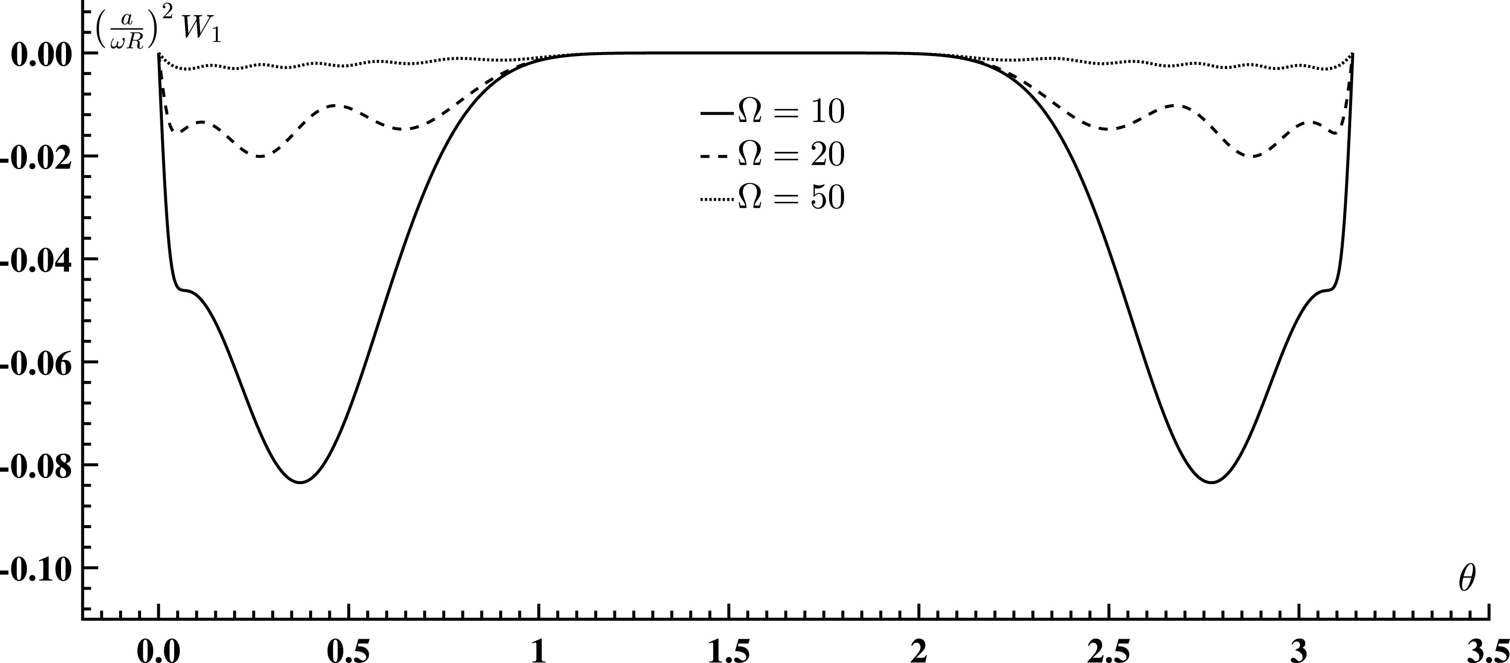
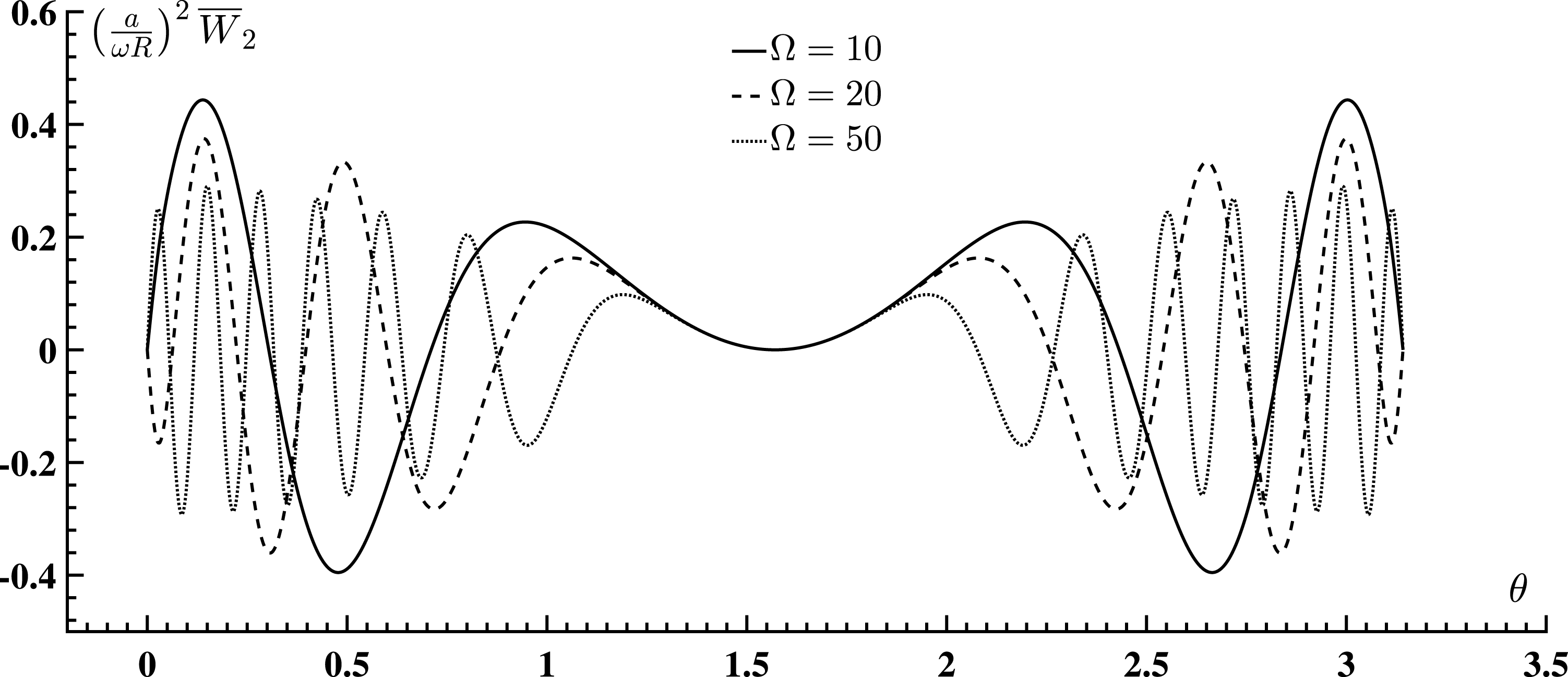
) are skew–symmetric, it is sufficient to plot them over half a circle. The figures that are indicated in table 2 correspond to the plots of the magnetic field and velocity perturbations.
Figures that represent both components of the magnetic field and velocity perturbations.

4.2 Polarisation relation and improvement of convergence
The series for the magnetic field perturbation spectrum (4.5a
) and (4.5b
) have a unit radius of convergence, and thus the coefficients (4.6a
) and (4.6b
) may be expected to be
 $O(1)$
as
 $n\rightarrow \infty$
; in this case the series obtained by differentiation (4.9a
) and (4.9b
) would diverge because the coefficients would be
 $O(n)$
as
 $n\rightarrow \infty$
, viz. it is well known that differentiation worsens the convergence of trigonometric series. The convergence would be improved, i.e. the coefficients would become
 $O(1/n)$
as
 $n\rightarrow \infty$
, by integration of (4.5a
) and (4.5b
), and to do this it is necessary to start from the polarisation relation (3.6a
) (instead of (3.6b
)), viz.
 $$\begin{eqnarray}H(\unicode[STIX]{x1D6FD};\unicode[STIX]{x1D714})=\frac{\text{i}}{\unicode[STIX]{x1D714}s}(BV)^{\prime }=\frac{\text{i}bR^{2}}{\unicode[STIX]{x1D714}s}\frac{\text{d}(V/s)}{\text{d}\unicode[STIX]{x1D6FD}},\end{eqnarray}$$
where (2.37) was used. From the equations (2.29) and (2.30) it follows that
 $$\begin{eqnarray}h(\unicode[STIX]{x1D703};\unicode[STIX]{x1D6FA})=\frac{\text{i}}{\unicode[STIX]{x1D714}R}\frac{\text{d}}{\text{d}\unicode[STIX]{x1D703}}\left[\sec ^{2}\unicode[STIX]{x1D703}V(\unicode[STIX]{x1D6FD};\unicode[STIX]{x1D714})\right],\end{eqnarray}$$
which, regarding the definition of the velocity perturbation spectrum, corresponds to
 $$\begin{eqnarray}h_{m}(\unicode[STIX]{x1D703};\unicode[STIX]{x1D6FA})=\left(\frac{a}{\unicode[STIX]{x1D714}R}\right)^{2}\frac{\text{d}}{\text{d}\unicode[STIX]{x1D703}}\left[\sec ^{2}\unicode[STIX]{x1D703}W_{m}(\unicode[STIX]{x1D703};\unicode[STIX]{x1D6FA})\right]\end{eqnarray}$$
and has to be integrated for
 $W_{m}$
, with (4.5a
) and (4.5b
) known. In the case
 $m=1$
, the integration of
 $$\begin{eqnarray}h_{1}(\unicode[STIX]{x1D703};\unicode[STIX]{x1D6FA})=\mathop{\sum }_{n=0}^{\infty }e_{n}\cos ^{2n+5}\unicode[STIX]{x1D703}=\left(\frac{a}{\unicode[STIX]{x1D714}R}\right)^{2}\frac{\text{d}}{\text{d}\unicode[STIX]{x1D703}}\left[\sec ^{2}\unicode[STIX]{x1D703}W_{1}(\unicode[STIX]{x1D703};\unicode[STIX]{x1D6FA})\right]\end{eqnarray}$$
can be made via the substitution
 $$\begin{eqnarray}\left(\frac{a}{\unicode[STIX]{x1D714}R}\right)^{2}W_{1}(\unicode[STIX]{x1D703};\unicode[STIX]{x1D6FA})=\sin \unicode[STIX]{x1D703}\mathop{\sum }_{n=0}^{\infty }\overline{e}_{n}\cos ^{2n+q}\unicode[STIX]{x1D703},\end{eqnarray}$$
with
 $\overline{e}_{n}$
and
 $q$
to be chosen, viz.
 $$\begin{eqnarray}\mathop{\sum }_{n=0}^{\infty }e_{n}\cos ^{2n+5}\unicode[STIX]{x1D703}=\mathop{\sum }_{n=0}^{\infty }\overline{e}_{n}\left[(2n+q-1)\cos ^{2n+q-1}\unicode[STIX]{x1D703}-(2n+q-2)\cos ^{2n+q-3}\unicode[STIX]{x1D703}\right],\end{eqnarray}$$
which is satisfied for
 $q=6$
, with
 $$\begin{eqnarray}q=6:\quad \mathop{\sum }_{n=0}^{\infty }\cos ^{2n+5}\unicode[STIX]{x1D703}\left[e_{n}-(2n+5)\overline{e}_{n}+(2n+6)\overline{e}_{n+1}\right]=0.\end{eqnarray}$$
Thus, the velocity perturbation spectra corresponding to (4.5a ) and (4.5b ) are respectively
 $$\begin{eqnarray}\displaystyle & \displaystyle \left(\frac{a}{\unicode[STIX]{x1D714}R}\right)^{2}W_{1}(\unicode[STIX]{x1D703};\unicode[STIX]{x1D6FA})=\sin \unicode[STIX]{x1D703}\mathop{\sum }_{n=1}^{\infty }\overline{e}_{n}\cos ^{2n+6}\unicode[STIX]{x1D703}, & \displaystyle\end{eqnarray}$$
 $$\begin{eqnarray}\displaystyle & \displaystyle \left(\frac{a}{\unicode[STIX]{x1D714}R}\right)^{2}W_{2}(\unicode[STIX]{x1D703};\unicode[STIX]{x1D6FA})=\sin \unicode[STIX]{x1D703}\mathop{\sum }_{n=1}^{\infty }\overline{f}_{n}\cos ^{2n-1}\unicode[STIX]{x1D703}, & \displaystyle\end{eqnarray}$$
 $$\begin{eqnarray}\displaystyle & \displaystyle e_{n}=(2n+5)\overline{e}_{n}-(2n+6)\overline{e}_{n+1}, & \displaystyle\end{eqnarray}$$
 $$\begin{eqnarray}\displaystyle & \displaystyle f_{n}=(2n-2)\overline{f}_{n}-(2n-1)\overline{f}_{n+1}, & \displaystyle\end{eqnarray}$$
 $q=6$
for (4.18a
) and
 $q=-1$
for (4.18b
). Note that the pairs of formulas (4.5a
) and (4.5b
), (4.17a
) and (4.17b
), (4.18a
) and (4.18b
) are similar replacing
 $2n+5$
by
 $2n-2$
. Also, setting
 $n=-1$
in (4.18a
) and (4.18b
) yields
 $\overline{e}_{0}=\overline{f}_{0}=0$
, so the series (4.17a
) and (4.17b
) start with
 $n=1$
; besides, setting
 $n=0$
in (4.18a
) and (4.18b
), the starting values of
 $\overline{e}_{1}$
and
 $\overline{f}_{1}$
are obtained,
 $$\begin{eqnarray}\overline{e}_{1}=-\frac{e_{0}}{6}=-\frac{1}{6},\quad \overline{f}_{1}=f_{0}=1,\end{eqnarray}$$
where the relations (4.5a
) and (4.5b
) were used. The successive coefficients
 $\overline{e}_{n+1}$
and
 $\overline{f}_{n+1}$
can be calculated from the preceding
 $\overline{e}_{n}$
and
 $\overline{f}_{n}$
, and from (4.6a
) and (4.6b
), that is, for
 $n=1,2,$
…, we have
 $$\begin{eqnarray}\overline{e}_{n+1}=\frac{(2n+5)\overline{e}_{n}-e_{n}}{2n+6},\quad \overline{f}_{n+1}=\frac{(2n-2)\overline{f}_{n}-f_{n}}{2n-1}.\end{eqnarray}$$
Thus all coefficients in the magnetic field and velocity perturbations spectra are specified.
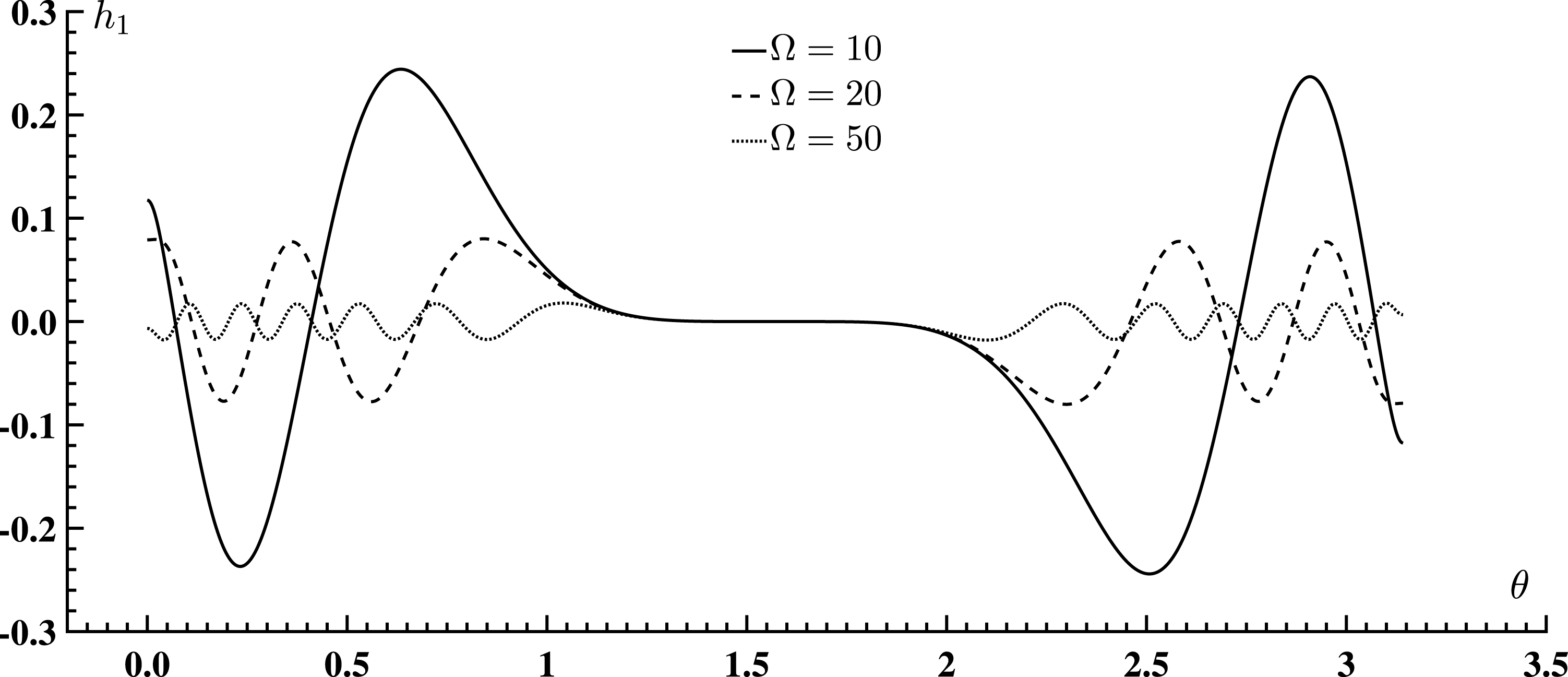
Component of magnetic field perturbation spectrum (4.5a
), which is finite over the whole circle, versus radial angle along a half-circle, for three values of the dimensionless frequency
 $\unicode[STIX]{x1D6FA}$
.


5 Discussion
The incompressibility condition
 $\unicode[STIX]{x1D735}\boldsymbol{\cdot }\boldsymbol{V}=0$
is met by these waves to
 $O(1/R)$
, according to (2.35); similarly, using (2.34) the force-free condition
 $$\begin{eqnarray}\unicode[STIX]{x1D735}\times (B(\unicode[STIX]{x1D6FD})\boldsymbol{e}_{\unicode[STIX]{x1D6FD}})=2\boldsymbol{e}_{z}s^{-2}\frac{\unicode[STIX]{x2202}(Bs)}{\unicode[STIX]{x2202}\unicode[STIX]{x1D6FC}}=2\boldsymbol{e}_{z}Bs^{-2}\frac{\unicode[STIX]{x2202}s}{\unicode[STIX]{x2202}\unicode[STIX]{x1D6FC}}=-4\unicode[STIX]{x1D6FC}B\boldsymbol{e}_{z}=-4\frac{B}{R}\boldsymbol{e}_{z}\end{eqnarray}$$
is met only to
 $O(1/R)$
. Gauss’ law for magnetism
 $\unicode[STIX]{x1D735}\boldsymbol{\cdot }\boldsymbol{h}=0$
is also met to
 $O(1/R)$
since
 $\unicode[STIX]{x1D735}\boldsymbol{\cdot }\boldsymbol{h}=-2h/R$
as in (2.35). Note that all these results arise because the scale factor
 $s=s(\unicode[STIX]{x1D6FC},\unicode[STIX]{x1D6FD})$
depends on both dipolar coordinates, according to (2.23). The criterion for Gauss’ law for magnetism
 $\unicode[STIX]{x1D735}\boldsymbol{\cdot }\boldsymbol{h}=0$
to be approximately satisfied may be chosen by
 $|\unicode[STIX]{x1D735}\boldsymbol{\cdot }\boldsymbol{h}|\ll |\unicode[STIX]{x1D735}\times \boldsymbol{h}|$
, where
 $\unicode[STIX]{x1D735}\times \boldsymbol{h}=\unicode[STIX]{x1D707}\boldsymbol{j}$
specifies the electric current associated with the Alfvén wave. Noting that
 $|\unicode[STIX]{x1D735}\times \boldsymbol{h}|\sim h\overline{k}=2\unicode[STIX]{x03C0}h/\unicode[STIX]{x1D706}$
where
 $\overline{k}$
is the wavenumber, and
 $\unicode[STIX]{x1D706}$
the wavelength, and
 $\unicode[STIX]{x1D735}\boldsymbol{\cdot }\boldsymbol{h}\sim h/R$
, it follows that
 $|\unicode[STIX]{x1D735}\boldsymbol{\cdot }\boldsymbol{h}|\ll |\unicode[STIX]{x1D735}\times \boldsymbol{h}|$
implies
 $1/R\ll 2\unicode[STIX]{x03C0}/\unicode[STIX]{x1D706}$
. Thus the Maxwell equation
 $|\unicode[STIX]{x1D735}\boldsymbol{\cdot }\boldsymbol{h}|=0$
is approximately satisfied; also, the pair of laws
 $\unicode[STIX]{x1D735}\boldsymbol{\cdot }\boldsymbol{v}=0$
and
 $\unicode[STIX]{x1D735}\times \boldsymbol{B}=\mathbf{0}$
is satisfied as well, if
 $1\ll 2\unicode[STIX]{x03C0}R/\unicode[STIX]{x1D706}=\unicode[STIX]{x1D714}R/a=\unicode[STIX]{x1D6FA}$
in terms of the dimensionless parameter
 $\unicode[STIX]{x1D6FA}$
.
Component of velocity perturbation spectrum (4.17a
), which is finite over the whole circle, versus radial angle along a half-circle, for three values of the dimensionless frequency
 $\unicode[STIX]{x1D6FA}$
.


A typical application of the present problem of Alfvén wave propagation in a dipolar magnetic field concerns planetary fields. In the case of the Earth, Alfvén waves in the ionosphere correspond to a gaseous background, and in the molten core, to a liquid incompressible medium. Taking for the ionospheric magnetic field
 $B_{0}=5.0\times 10^{-9}~\text{T}$
at approximately the Earth’s radius
 $R_{0}=6.4\times 10^{6}~\text{m}$
, in the core at one tenth of the radius
 $R_{1}=0.1R_{0}=6.4\times 10^{5}~\text{m}$
a dipolar magnetic field, which scales like the inverse cube of distance
 ${\sim}1/R^{3}$
, is one thousand times bigger
 $B_{1}=10^{3}B_{0}=5.0\times 10^{-6}~\text{T}$
. For a mass density
 $\unicode[STIX]{x1D70C}=5.5\times 10^{3}~\text{kg}~\text{m}^{-3}$
and the value of magnetic permeability equal to the permeability of the free space, this leads to a small Alfvén speed
 $a_{1}=B_{1}/\sqrt{\unicode[STIX]{x1D707}\unicode[STIX]{x1D70C}}=6.0\times 10^{-5}~\text{m}~\text{s}^{-1}$
. Taking the period of one day,
 $\unicode[STIX]{x1D70F}=24\times 3600~\text{s}=8.64\times 10^{4}~\text{s}$
, or frequency
 $\unicode[STIX]{x1D714}=2\unicode[STIX]{x03C0}/\unicode[STIX]{x1D70F}=7.3\times 10^{-5}~\text{s}^{-1}$
, leads to the value
 $\unicode[STIX]{x1D6FA}_{1}=\unicode[STIX]{x1D714}R_{1}/a_{1}=7.7\times 10^{5}\gg 1$
, which meets the conditions stated in the preceding paragraph. As a second example, deeper in the core, at one hundredth of the Earth’s radius
 $R_{2}=10^{-2}R_{0}=6.4\times 10^{4}~\text{m}$
, the magnetic field
 $B_{2}=10^{6}B_{0}=5.0\times 10^{-3}~\text{T}$
leads to an Alfvén speed
 $a_{2}=B_{2}/\sqrt{\unicode[STIX]{x1D707}\unicode[STIX]{x1D70C}}=6.0\times 10^{-2}~\text{m}~\text{s}^{-2}$
. The corresponding value of the parameter
 $\unicode[STIX]{x1D6FA}_{2}=\unicode[STIX]{x1D714}R_{2}/a_{2}=7.8\times 10^{1}$
still meets the condition
 $\unicode[STIX]{x1D6FA}\gg 1$
.
For the purpose of illustration of the velocity and magnetic field perturbations, the parameter is given by the values
 $$\begin{eqnarray}\unicode[STIX]{x1D6FA}=10,20,50,\end{eqnarray}$$
which satisfy
 $\unicode[STIX]{x1D6FA}\gg 1$
, and also given the symmetries of the fields over the full circle
 $0\leqslant \unicode[STIX]{x1D703}\leqslant 2\unicode[STIX]{x03C0}$
, only one half is plotted,
 $0\leqslant \unicode[STIX]{x1D703}\leqslant \unicode[STIX]{x03C0}$
. Note that since
 $\unicode[STIX]{x1D703}=\unicode[STIX]{x03C0}/2$
corresponds to the magnetic north pole, the range for plotting
 $0\leqslant \unicode[STIX]{x1D703}\leqslant \unicode[STIX]{x03C0}$
corresponds to the upper hemisphere. Starting with the magnetic field perturbation and the component (4.5a
), which is finite over the whole circle
 $0\leqslant \unicode[STIX]{x1D703}\leqslant 2\unicode[STIX]{x03C0}$
, it is a symmetric function of
 $\unicode[STIX]{x1D703}$
, and hence the plot over the northern hemisphere (figure 3) can be repeated on the lower hemisphere by symmetry on the equator. The field vanishes at the magnetic poles
 $H_{1}(\pm \unicode[STIX]{x03C0}/2;\unicode[STIX]{x1D6FA})=0$
, and is skew–symmetric relative to the polar axis because
 $H_{1}(\unicode[STIX]{x03C0}/2-\unicode[STIX]{x1D703};\unicode[STIX]{x1D6FA})=-H_{1}(\unicode[STIX]{x03C0}/2+\unicode[STIX]{x1D703};\unicode[STIX]{x1D6FA})$
. Away from the poles
 $\unicode[STIX]{x1D703}=\pm \unicode[STIX]{x03C0}/2$
, i.e. towards the equator
 $\unicode[STIX]{x1D703}=0$
or
 $\unicode[STIX]{x1D703}=\unicode[STIX]{x03C0}$
, the magnetic field perturbation oscillates with smaller amplitude, and shorter wavelength, for larger
 $\unicode[STIX]{x1D6FA}$
.
The component (4.5b
) of the magnetic field perturbation is unbounded at the poles
 $\unicode[STIX]{x1D703}=\pm \unicode[STIX]{x03C0}/2$
. Thus, the general wavefield
 $$\begin{eqnarray}h(\unicode[STIX]{x1D703};\unicode[STIX]{x1D6FA})=C_{1}^{\star }h_{1}(\unicode[STIX]{x1D703};\unicode[STIX]{x1D6FA})+C_{2}^{\star }h_{2}(\unicode[STIX]{x1D703};\unicode[STIX]{x1D6FA})\end{eqnarray}$$
is finite over the whole circle only if
 $C_{2}^{\star }=0$
is met, in which case the remaining constant of integration
 $C_{1}^{\star }$
can be determined using
 $$\begin{eqnarray}h(0;\unicode[STIX]{x1D6FA})=C_{1}^{\star }\mathop{\sum }_{n=0}^{\infty }e_{n}\end{eqnarray}$$
and knowing the magnetic field perturbation spectrum
 $h(0;\unicode[STIX]{x1D6FA})$
at
 $\unicode[STIX]{x1D703}=0$
. It follows that the dimensionless magnetic field perturbation is a constant multiple
 $C_{1}^{\star }$
of
 $h_{1}(\unicode[STIX]{x1D703};\unicode[STIX]{x1D6FA})$
plotted in figure 3. In order to plot
 $h_{2}(\unicode[STIX]{x1D703};\unicode[STIX]{x1D6FA})$
it is convenient to remove the singularity at
 $\unicode[STIX]{x1D703}=\pm \unicode[STIX]{x03C0}/2$
, by inserting the factor
 $\cos ^{2}\unicode[STIX]{x1D703}$
, viz.
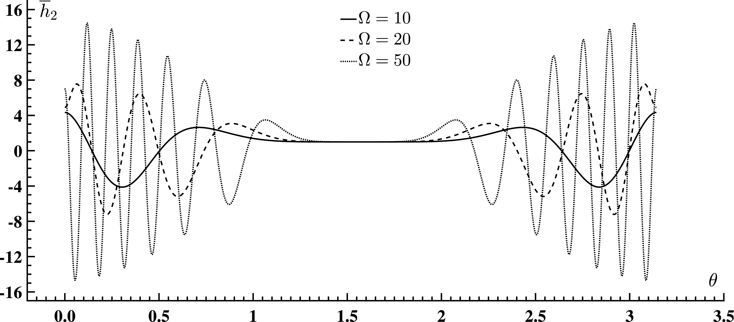
 $$\begin{eqnarray}\overline{h}_{2}(\unicode[STIX]{x1D703};\unicode[STIX]{x1D6FA})\equiv \cos ^{2}\unicode[STIX]{x1D703}h_{2}(\unicode[STIX]{x1D703};\unicode[STIX]{x1D6FA})=\mathop{\sum }_{n=0}^{\infty }f_{n}\cos ^{2n}\unicode[STIX]{x1D703}.\end{eqnarray}$$
The magnetic field perturbation is symmetric on the southern and northern hemispheres. It vanishes at the poles,
 $\overline{H}_{2}(\pm \unicode[STIX]{x03C0}/2;\unicode[STIX]{x1D6FA})=0$
, is symmetric relative to the polar axis,
 $\overline{H}_{2}(\unicode[STIX]{x03C0}/2-\unicode[STIX]{x1D703};\unicode[STIX]{x1D6FA})=\overline{H}_{2}(\unicode[STIX]{x03C0}/2+\unicode[STIX]{x1D703};\unicode[STIX]{x1D6FA})$
, and oscillates with larger amplitude and shorter wavelength for larger
 $\unicode[STIX]{x1D6FA}$
(figure 4). The range of values of
 $\overline{h}_{2}$
in figure 4 is more than one order of magnitude larger than the range of values of
 $h_{1}$
in figure 3, so the latter is plotted separately to aid visibility. Comparing
 $H_{1}$
and
 $\overline{H}_{2}$
as
 $\unicode[STIX]{x1D6FA}$
increases, there are more nodes for both; also, as
 $\unicode[STIX]{x1D6FA}$
increases the amplitude decreases for
 $H_{1}$
and increases for
 $\overline{H}_{2}$
.
Concerning the component of the velocity perturbation (4.9a
) which is finite over the whole circle
 $0\leqslant \unicode[STIX]{x1D703}\leqslant 2\unicode[STIX]{x03C0}$
, it is skew–symmetric,
 $W_{1}(\unicode[STIX]{x1D703};\unicode[STIX]{x1D6FA})=-W_{1}(-\unicode[STIX]{x1D703};\unicode[STIX]{x1D6FA})$
, so that in the lower hemisphere it has the opposite sign to the upper hemisphere (figure 5). It vanishes at the magnetic poles and equator
 $\unicode[STIX]{x1D703}=\pm \unicode[STIX]{x03C0}/2,0,\unicode[STIX]{x03C0}$
, and is symmetric relative to the polar axis because
 $W_{1}(\unicode[STIX]{x03C0}/2+\unicode[STIX]{x1D703};\unicode[STIX]{x1D6FA})=W_{1}(\unicode[STIX]{x03C0}/2-\unicode[STIX]{x1D703};\unicode[STIX]{x1D6FA})$
. For
 $\unicode[STIX]{x1D6FA}=10$
there is a single large extremum, and on increasing
 $\unicode[STIX]{x1D6FA}$
the number of local extrema increases and their magnitude decreases. The other component of the velocity perturbation spectrum (4.9b
) is singular at the magnetic poles
 $\unicode[STIX]{x1D703}=\pm \unicode[STIX]{x03C0}/2$
. The singularity is suppressed by inserting a suitable factor,
 $$\begin{eqnarray}\left(\frac{a}{\unicode[STIX]{x1D714}R}\right)^{2}\overline{W}_{2}(\unicode[STIX]{x1D703};\unicode[STIX]{x1D6FA})\equiv \left(\frac{a}{\unicode[STIX]{x1D714}R}\right)^{2}\cos \unicode[STIX]{x1D703}W_{2}(\unicode[STIX]{x1D703};\unicode[STIX]{x1D6FA})=\sin \unicode[STIX]{x1D703}\mathop{\sum }_{n=0}^{\infty }\overline{f}_{n}\cos ^{2n}\unicode[STIX]{x1D703}.\end{eqnarray}$$
The velocity perturbation is a skew–symmetric function of
 $\unicode[STIX]{x1D703}$
, i.e. has opposite signs in the upper and lower hemispheres. It vanishes at the magnetic poles and equator, and is symmetric relative to the polar axis (figures 5 and 6). For increasing
 $\unicode[STIX]{x1D6FA}$
the wavelength is larger and the amplitude of oscillations also larger. Comparing
 $W_{1}$
and
 $\overline{W}_{2}$
it is clear that there are more oscillations for both as
 $\unicode[STIX]{x1D6FA}$
increases; for increasing
 $\unicode[STIX]{x1D6FA}$
the amplitude is smaller for
 $W_{1}$
and larger for
 $\overline{W}_{2}$
. Also
 $\overline{W}_{2}$
has oscillatory sign, i.e. is alternatively positive and negative, whereas
 $W_{1}$
is always negative.
In figures 3–6, the circular magnetic field lines are described from
 $\unicode[STIX]{x1D703}=0$
to
 $\unicode[STIX]{x1D703}=\unicode[STIX]{x03C0}$
. If the field lines (and magnetic poles) do not follow the geographical positioning, that is, if the field lines would not be measured between
 $0$
and
 $\unicode[STIX]{x03C0}$
, the effect on the propagation of Alfvén waves would be a translation
 $\unicode[STIX]{x1D703}\rightarrow \unicode[STIX]{x1D703}+\unicode[STIX]{x1D703}_{0}$
and therefore it would lead to different starting values.
Since one component, each of the magnetic and velocity perturbations, is singular, a suitable factor was introduced to obtain a finite value and to make the plots in figures 4 and 6 visible over the whole range of values
 $0<\unicode[STIX]{x1D703}<\unicode[STIX]{x03C0}$
. The scale in figure 4 would be larger without this factor, and could be reduced by an additional constant factor like 0.1. In all cases of figures 3–6 the objective was to plot the dependence of the wavefields visibly along the whole of the circular magnetic field lines of a dipole for several values of the dimensionless frequency.
The main feature of this paper is to consider the Alfvén wave propagation along a closed magnetic field line, in fact the simplest closed curve: the circle. In situations in which the closed magnetic field is not a circle, like the magnetic field of the Earth, Sun and other planets and stars, the local curvature would replace the radius of the circle; this approximation is valid if the wavelength is much smaller than the length scale of the change of curvature
 $$\begin{eqnarray}\unicode[STIX]{x1D706}=\frac{2\unicode[STIX]{x03C0}}{k}\leqslant \frac{R(\unicode[STIX]{x1D703})}{R^{\prime }(\unicode[STIX]{x1D703})}=\frac{\text{d}}{\text{d}\unicode[STIX]{x1D703}}\{\log [R(\unicode[STIX]{x1D703})]\},\end{eqnarray}$$
where
 $R(\unicode[STIX]{x1D703})$
is the radius of curvature at the angular position
 $\unicode[STIX]{x1D703}$
of the closed magnetic field line.
The present model considers a constant Alfvén speed (2.42) with the direction varying along a circle. The case of an Alfvén wave propagating with constant direction and varying Alfvén speed has been studied in detail in the case of atmospheres like the Sun and radial flows like the solar wind (see references in the third paragraph of the § 1). An Alfvén speed increasing with distance leads to a waveform stretching with increasing spacing of the nodes, smaller waveform slope and less dissipation; the reverse occurs for Alfvén speed decreasing with distance.
Acknowledgements
This work was supported by the FCT (Fundação para a Ciência e Tecnologia) through IDMEC (Institute of Mechanical Engineering), under LAETA Pest -OE/EME/LA0022. The authors thank Ms N. L. Isaeva for her contribution to an early version of this work. The authors also thank the two reviewers who read the article and gave comments and questions during the publication process which helped to improve the manuscrispt.
Appendix A. Multipolar expansion for the steady magnetic field
The Maxwell equations for the steady magnetic field (assuming
 $\unicode[STIX]{x2202}/\unicode[STIX]{x2202}t=0$
), particularly the Ampère–Maxwell equation and Gauss’ law for magnetism, are
 $$\begin{eqnarray}\displaystyle & \displaystyle \unicode[STIX]{x1D735}\times \boldsymbol{H}=\boldsymbol{J}, & \displaystyle\end{eqnarray}$$
 $$\begin{eqnarray}\displaystyle & \displaystyle \unicode[STIX]{x1D735}\boldsymbol{\cdot }\boldsymbol{B}=0, & \displaystyle\end{eqnarray}$$
 $\boldsymbol{H}$
is the magnetic field,
 $\boldsymbol{B}$
is the magnetic induction and
 $\boldsymbol{J}$
is the electric current density per unit volume. For an isotropic medium with constant magnetic permeability (
 $\unicode[STIX]{x1D707}=\text{const.}$
), the constitutive relation
 $$\begin{eqnarray}\boldsymbol{B}=\unicode[STIX]{x1D707}\boldsymbol{H}\end{eqnarray}$$
leads to
 $$\begin{eqnarray}\unicode[STIX]{x1D735}\boldsymbol{\cdot }\boldsymbol{H}=0.\end{eqnarray}$$
Using the vector identity
 $$\begin{eqnarray}\unicode[STIX]{x1D735}^{2}\boldsymbol{H}=\unicode[STIX]{x1D735}(\unicode[STIX]{x1D735}\boldsymbol{\cdot }\boldsymbol{H})-\unicode[STIX]{x1D735}\times (\unicode[STIX]{x1D735}\times \boldsymbol{H}),\end{eqnarray}$$
the curl of (A 1a ) is given by
 $$\begin{eqnarray}\unicode[STIX]{x1D735}\times \boldsymbol{J}=\unicode[STIX]{x1D735}\times (\unicode[STIX]{x1D735}\times \boldsymbol{H}),\end{eqnarray}$$
leading to
 $$\begin{eqnarray}\unicode[STIX]{x1D735}\times \boldsymbol{J}=-\unicode[STIX]{x1D735}^{2}\boldsymbol{H},\end{eqnarray}$$
by use of the equations (A 3) and (A 2b ). Thus the steady magnetic field satisfies a vector Poisson equation
 $$\begin{eqnarray}\unicode[STIX]{x1D735}^{2}\boldsymbol{H}=\boldsymbol{Q}\end{eqnarray}$$
forced by the curl of the electric current
 $$\begin{eqnarray}\boldsymbol{Q}=-\unicode[STIX]{x1D735}\times \boldsymbol{J}.\end{eqnarray}$$
For a distribution of electric currents over a domain
 ${\mathcal{D}}$
with source coordinates
 $\boldsymbol{y}$
, the magnetic field at an observer position
 $\boldsymbol{x}$
is given by the Poisson integral
 $$\begin{eqnarray}\boldsymbol{H}(\boldsymbol{x})=\frac{1}{4\unicode[STIX]{x03C0}}\int _{{\mathcal{D}}}\frac{\boldsymbol{Q}(\boldsymbol{y})}{|\boldsymbol{x}-\boldsymbol{y}|}~\text{d}^{3}\boldsymbol{y}.\end{eqnarray}$$
If the observer
 $\boldsymbol{x}$
lies outside the source
 $\boldsymbol{y}$
region, the distance
 $|\boldsymbol{x}-\boldsymbol{y}|$
is not zero and its inverse may be expanded in a Maclaurin series of powers of
 $\boldsymbol{y}$
around
 $\boldsymbol{y}=\mathbf{0}$
 $$\begin{eqnarray}\frac{1}{|\boldsymbol{x}-\boldsymbol{y}|}=\frac{1}{|\boldsymbol{x}|}+\mathop{\sum }_{n=1}^{\infty }\frac{M_{n}}{|\boldsymbol{x}|^{n}}\end{eqnarray}$$
with coefficients
 $$\begin{eqnarray}M_{n}(\boldsymbol{x},\boldsymbol{y})=\mathop{\sum }_{i_{1},\ldots ,i_{n}=1}^{3}y_{i_{1}}\cdots y_{i_{n}}\lim _{\boldsymbol{y}\rightarrow \mathbf{0}}\frac{\unicode[STIX]{x2202}^{n}}{\unicode[STIX]{x2202}y_{i_{1}}\cdots \unicode[STIX]{x2202}y_{i_{n}}}\left(\frac{1}{|\boldsymbol{x}-\boldsymbol{y}|}\right).\end{eqnarray}$$
Substitution of (A 8) in (A 6) leads to the multipolar expansion
 $$\begin{eqnarray}\boldsymbol{H}(\boldsymbol{x})=\frac{\boldsymbol{N}_{0}}{|\boldsymbol{x}|}+\mathop{\sum }_{n=1}^{\infty }\frac{\boldsymbol{N}_{n}}{|\boldsymbol{x}|^{n}},\end{eqnarray}$$
showing that the magnetic field is the sum of a series of inverse powers of the distance with: (I) lowest-order vector coefficient
 $$\begin{eqnarray}\boldsymbol{N}_{0}=\int _{{\mathcal{D}}}\boldsymbol{Q}(\boldsymbol{y})~\text{d}^{3}\boldsymbol{y}\end{eqnarray}$$
specified by the integral of the ‘source’ term (A 5b ) in (A 5a ) over the domain, corresponding to a dipole; (II) the remaining terms in (A 9) that are higher-order multipoles with moments given by
 $$\begin{eqnarray}\boldsymbol{N}_{n}=\int _{\unicode[STIX]{x2202}{\mathcal{D}}}\boldsymbol{Q}(\boldsymbol{y})M_{n}(\boldsymbol{x},\boldsymbol{y})~\text{d}^{3}\boldsymbol{y}\end{eqnarray}$$
involving the source term (A 5b
) and the relative positions of source and observer (A 8). In the near field for small
 $|\boldsymbol{x}|$
, all terms in the multipolar expansion (A 9) have to be considered. In the far field for large
 $|\boldsymbol{x}|$
, the multipolar expansion (A 9) is dominated by the lowest-order dipole term (A 10a
).
The translation of plane dipolar coordinates (figure 1) along the normal to their plane leads to cylindrical dipolar coordinates whose coordinate surfaces are: (I) a cylinder with vertical axis passing through the
 $x$
coordinate axis and a generator along the
 $z$
axis; (II) another cylinder with vertical axis passing through the
 $y$
coordinate axis and a generator along the
 $z$
axis; (III) horizontal plane that is orthogonal to both families of cylinders that are also orthogonal to each other.

Appendix B. Cylindrical and spherical dipolar coordinates
The plane dipolar coordinates can be extended to three dimensions as cylindrical dipolar coordinates (
 $\unicode[STIX]{x1D6FC}$
,
 $\unicode[STIX]{x1D6FD}$
,
 $z$
) by adding an orthogonal Cartesian coordinate
 $z$
with unit scale factor
 $$\begin{eqnarray}h_{z}=1.\end{eqnarray}$$
Thus, the cylindrical dipolar coordinates where
 $z$
is a Cartesian axis orthogonal to the (
 $\unicode[STIX]{x1D6FC}$
,
 $\unicode[STIX]{x1D6FD}$
) plane,
 $$\begin{eqnarray}(\text{d}l)^{2}=s^{2}\left[(\text{d}\unicode[STIX]{x1D6FC})^{2}+(\text{d}\unicode[STIX]{x1D6FD})^{2}\right]+\left(h_{z}\right)^{2}(\text{d}z)^{2},\end{eqnarray}$$
have arclength equal to
 $$\begin{eqnarray}(\text{d}l)^{2}=\frac{1}{\unicode[STIX]{x1D6FC}^{2}+\unicode[STIX]{x1D6FD}^{2}}\left[(\text{d}\unicode[STIX]{x1D6FC})^{2}+(\text{d}\unicode[STIX]{x1D6FD})^{2}\right]+(\text{d}z)^{2}.\end{eqnarray}$$
The coordinate surfaces (figure 7) are: (I)
 $\unicode[STIX]{x1D6FC}=\text{const.}$
as a cylinder, with axis parallel to the
 $OZ$
-axis, passing through the
 $OX$
-axis at
 $(1/(2\unicode[STIX]{x1D6FC}),0,0)$
, with radius
 $1/(2\unicode[STIX]{x1D6FC})$
, so that the
 $OZ$
-axis is a generator; (II)
 $\unicode[STIX]{x1D6FD}=\text{const.}$
that is also a cylinder, with axis parallel to the
 $OZ$
-axis, passing through the
 $OX$
-axis at
 $(0,1/(2\unicode[STIX]{x1D6FD}),0)$
, with radius
 $1/(2\unicode[STIX]{x1D6FD})$
, so that the
 $OZ$
-axis is a generator; (III) a plane
 $z=\text{const.}$
, orthogonal to the
 $\unicode[STIX]{x1D6FC}$
and
 $\unicode[STIX]{x1D6FD}$
cylinders. The coordinate curves are: (I)
 $\unicode[STIX]{x1D6FC},z=\text{const.}$
as a circle, on the plane
 $z=\text{const.}$
, with centre at
 $(1/(2\unicode[STIX]{x1D6FC}),0,z)$
, and radius
 $1/(2\unicode[STIX]{x1D6FC})$
, touching the
 $OZ$
-axis at
 $(0,0,z)$
; (II)
 $\unicode[STIX]{x1D6FD},z=\text{const.}$
as a circle, on the plane
 $z=\text{const.}$
, with centre at
 $(0,1/(2\unicode[STIX]{x1D6FD}),z)$
, and radius
 $1/(2\unicode[STIX]{x1D6FD})$
, touching the
 $OZ$
-axis at
 $(0,0,z)$
; (III) and
 $\unicode[STIX]{x1D6FC},\unicode[STIX]{x1D6FD}=\text{const.}$
as a straight line parallel to the
 $OZ$
-axis, passing through the point
 $(\unicode[STIX]{x1D6FC},\unicode[STIX]{x1D6FD},0)$
, which is the common generator of the two cylinders
 $\unicode[STIX]{x1D6FC},\unicode[STIX]{x1D6FD}=\text{const}$
.
Rotating the plane dipolar coordinates (figure 1) around the
 $x$
axis leads to spherical dipolar coordinates whose coordinate surfaces are: (I) a sphere
 $\unicode[STIX]{x1D6FC}=\text{const.}$
with centre on the
 $x$
axis passing through the origin; (II) a torus
 $\unicode[STIX]{x1D6FD}=\text{const.}$
with the origin as the interior point where touch all circular cross-sections through planes passing through the
 $x$
axis; (III) any plane
 $\unicode[STIX]{x1D719}=\text{const.}$
that pass through the
 $x$
axis and is orthogonal both to the sphere (I) and torus (II).

Spherical dipolar coordinates (
 $\unicode[STIX]{x1D6FC}$
,
 $\unicode[STIX]{x1D6FD}$
,
 $\unicode[STIX]{x1D719}$
) are obtained by rotating plane dipolar coordinates (
 $\unicode[STIX]{x1D6FC}$
,
 $\unicode[STIX]{x1D6FD}$
) around the
 $OX$
-axis, thus adding as third coordinate the azimuthal angle
 $\unicode[STIX]{x1D719}$
whose corresponding scale factor is
 $$\begin{eqnarray}h_{\unicode[STIX]{x1D719}}=r\sin \unicode[STIX]{x1D703}=\frac{\unicode[STIX]{x1D6FD}}{\unicode[STIX]{x1D6FC}^{2}+\unicode[STIX]{x1D6FD}^{2}}=\unicode[STIX]{x1D6FD}s,\end{eqnarray}$$
where (2.20b ) and (2.23) were used. The arclength
 $$\begin{eqnarray}(\text{d}l)^{2}=s^{2}\left[(\text{d}\unicode[STIX]{x1D6FC})^{2}+(\text{d}\unicode[STIX]{x1D6FD})^{2}\right]+\left(h_{\unicode[STIX]{x1D719}}\right)^{2}(\text{d}\unicode[STIX]{x1D719})^{2}=s^{2}\left[(\text{d}\unicode[STIX]{x1D6FC})^{2}+(\text{d}\unicode[STIX]{x1D6FD})^{2}+\unicode[STIX]{x1D6FD}^{2}(\text{d}\unicode[STIX]{x1D719})^{2}\right]\end{eqnarray}$$
is given by
 $$\begin{eqnarray}(\text{d}l)^{2}=\frac{1}{\left(\unicode[STIX]{x1D6FC}^{2}+\unicode[STIX]{x1D6FD}^{2}\right)^{2}}\left[(\text{d}\unicode[STIX]{x1D6FC})^{2}+(\text{d}\unicode[STIX]{x1D6FD})^{2}+\unicode[STIX]{x1D6FD}^{2}(\text{d}\unicode[STIX]{x1D719})^{2}\right].\end{eqnarray}$$
The coordinate surfaces (figure 8) are: (I)
 $\unicode[STIX]{x1D6FC}=\text{const.}$
as a sphere, with centre on the
 $OX$
-axis at
 $(1/(2\unicode[STIX]{x1D6FC}),0,0)$
and radius
 $1/(2\unicode[STIX]{x1D6FC})$
, so that it is tangent to the
 $YOZ$
plane at the origin; (II)
 $\unicode[STIX]{x1D6FD}=\text{const.}$
as a torus, with cross-section a circle of radius
 $1/(2\unicode[STIX]{x1D6FD})$
, along the
 $OX$
-axis, and line of centres a circle in the
 $YOZ$
-plane, of radius
 $1/(2\unicode[STIX]{x1D6FD})$
and centre at the origin, so the torus touches itself at the origin; (III)
 $\unicode[STIX]{x1D719}=\text{const.}$
as a semi-plane, passing through the
 $OX$
-axis, and making an angle
 $\unicode[STIX]{x1D719}$
with the
 $OZ$
-axis. The coordinate curves are: (I)
 $\unicode[STIX]{x1D6FC},\unicode[STIX]{x1D719}=\text{const.}$
as a circle of radius
 $1/(2\unicode[STIX]{x1D6FC})$
with centre on the plane
 $\unicode[STIX]{x1D719}=\text{const.}$
at a distance
 $1/(2\unicode[STIX]{x1D6FC})$
from the
 $OY$
-axis, to which it is tangent; (II)
 $\unicode[STIX]{x1D6FD},\unicode[STIX]{x1D719}=\text{const.}$
as a circle of radius
 $1/(2\unicode[STIX]{x1D6FD})$
with centre on the plane
 $\unicode[STIX]{x1D719}=\text{const.}$
at a distance
 $1/(2\unicode[STIX]{x1D6FD})$
from the
 $OX$
-axis, to which it is tangent; (III)
 $\unicode[STIX]{x1D6FC},\unicode[STIX]{x1D6FD}=\text{const.}$
as a circle on a plane perpendicular to the
 $OX$
-axis, at a distance
 $r$
from the origin, with centre on the
 $OX$
-axis at
 $(x,0,0)$
and radius
 $y$
given by
 $$\begin{eqnarray}\displaystyle & \displaystyle x=r\cos \unicode[STIX]{x1D703}=r^{2}\unicode[STIX]{x1D6FC}=\frac{\unicode[STIX]{x1D6FC}}{\left|\unicode[STIX]{x1D6FC}^{2}+\unicode[STIX]{x1D6FD}^{2}\right|}, & \displaystyle\end{eqnarray}$$
 $$\begin{eqnarray}\displaystyle & \displaystyle y=r\sin \unicode[STIX]{x1D703}=r^{2}\unicode[STIX]{x1D6FD}=\frac{\unicode[STIX]{x1D6FD}}{\left|\unicode[STIX]{x1D6FC}^{2}+\unicode[STIX]{x1D6FD}^{2}\right|}, & \displaystyle\end{eqnarray}$$